1

NATIONAL TECHNICAL UNIVERSITY OF ATHENS

School of Naval Architecture and Marine Engineering

Sector of Ship Design and Maritime Transport

Supervising Professor: Nikolaos Themelis

Evaluation of Design and Operational

measures to meet IMO 2050 targets for

Containerships

Diploma Thesis of

Gerasimos Michalopoulos

September 2021

2

Περίληψη

Η παρούσα διπλωματική εργασία αποσκοπεί στην μελέτη των διαθέσιμων εναλλακτικών μείωσης

των εκπομπών του θερμοκηπίου με σκοπό τη συμμόρφωση με τους κανονισμούς του Διεθνή

Ναυτιλιακού Οργανισμού, ΙΜΟ. Ο τύπος πλοίου που θα απασχολήσει το μεγαλύτερο Κεφάλαιο

αυτής της εργασίας είναι τα πλοία μεταφοράς εμπορευματοκιβωτίων. Η συγκεκριμένη κατηγορία

πλοίων παράγει τις μεγαλύτερες εκπομπές ανά μεταφερόμενο έργο, λόγω των μεγάλων

υπηρεσιακών ταχυτήτων της και για το λόγo αυτό έχει τα μεγαλύτερα περιθώρια βελτίωσης. Ο

κύριος στόχος αυτής της εργασίας, είναι η διερεύνηση της επίδρασης κάθε εναλλακτικής στις

εκπομπές του θερμοκηπίου και η αξιολόγησή της μέσω δεικτών απόδοσης και οικονομικής

ανάλυσης.

Η ανάλυση αυτής της διπλωματικής γίνεται σε τρία Κεφάλαια με το καθένα να έχει συνάφεια με

τα υπόλοιπα αλλά διαφορετική θεματολογία.

Στο Κεφάλαιο 2 γίνεται μια σύντομη ανασκόπηση των κανονισμών του ΙΜΟ. Οι κλιμάκωση

αυτών των κανονισμών τοποθετείται στο έτος 2050, όπου ο οργανισμός στοχεύει στη μείωση των

συνολικά παραγόμενων εκπομπών του θερμοκηπίου από τη ναυτιλία στο 50% των επιπέδων που

βρίσκονταν το 2008. Κάτι τέτοιο θεωρείτε εφικτό με βελτίωση της αποδοτικότητας των πλοίων

κατά 70%. Για την επίτευξη αυτής την μεγάλης αύξησης αποδοτικότητας, ένας μεγάλος αριθμών

εναλλακτικών έχουν προταθεί, αρκετές από τις οποίες αναλύονται στα επόμενα κεφάλαια.

Στο Κεφάλαιο 3 γίνεται μια ανασκόπηση της βιβλιογραφίας των διαθέσιμων εναλλακτικών για τις

οποίες δεν υπήρχαν αρκετά δεδομένα για να πραγματοποιηθεί μελέτη περίπτωσης. Αξίζει να

σημειωθεί ότι οι περισσότερες εναλλακτικές δεν μπορούν από μόνες τους να επιφέρουν την

προτεινόμενη αλλαγή.

Στο Κεφάλαιο 4 πραγματοποιήθηκε η μελέτη περίπτωσης για τρεις εναλλακτικές που επιλέχθηκαν

για τον τύπο πλοίου που μελετάται, εμπορευματοκιβώτια από σύνθετα υλικά, μείωση της

ταχύτητας λειτουργίας και οικονομίες κλίμακας από τη χρήση μεγαλύτερων πλοίων. Για την

αξιολόγηση των αποτελεσμάτων των δύο πρώτων εναλλακτικών υπήρξε αλλαγή στο λειτουργικό

προφίλ του πλοίου και για το λόγο αυτό έγινε χρήση προγραμμάτων πρόβλεψης αντίστασης

(NavCad) και πρόωσης (PropulsionMCR). Σε όλες τις περιπτώσεις έγινε κατάλληλη χρήση του

συνόλου των διαθέσιμων δεδομένων για ένα πλοίο μεταφοράς εμπορευματοκιβωτίων τύπου

Panamax, ενώ όπου ήταν εφικτό έγινε αξιολόγηση μέσω κατάλληλων δεικτών και οικονομικής

ανάλυσης.

Τέλος, τα συμπεράσματα και οι προτάσεις για περαιτέρω έρευνα αυτής της εργασίας βρίσκονται

στο Κεφάλαιο 5 ενώ μερικές επιπρόσθετες πληροφορίες μπορούν να βρεθούν στο Παράρτημα –

Κεφάλαιο 7.

3

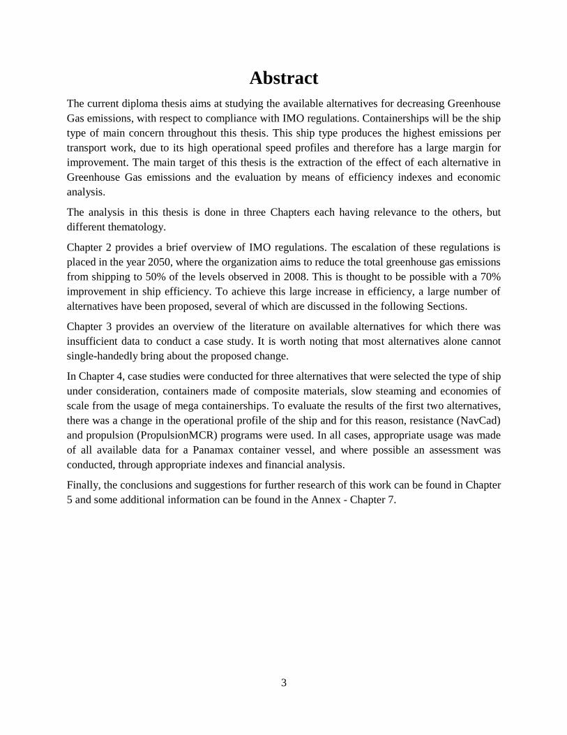
Abstract

The current diploma thesis aims at studying the available alternatives for decreasing Greenhouse

Gas emissions, with respect to compliance with IMO regulations. Containerships will be the ship

type of main concern throughout this thesis. This ship type produces the highest emissions per

transport work, due to its high operational speed profiles and therefore has a large margin for

improvement. The main target of this thesis is the extraction of the effect of each alternative in

Greenhouse Gas emissions and the evaluation by means of efficiency indexes and economic

analysis.

The analysis in this thesis is done in three Chapters each having relevance to the others, but

different thematology.

Chapter 2 provides a brief overview of IMO regulations. The escalation of these regulations is

placed in the year 2050, where the organization aims to reduce the total greenhouse gas emissions

from shipping to 50% of the levels observed in 2008. This is thought to be possible with a 70%

improvement in ship efficiency. To achieve this large increase in efficiency, a large number of

alternatives have been proposed, several of which are discussed in the following Sections.

Chapter 3 provides an overview of the literature on available alternatives for which there was

insufficient data to conduct a case study. It is worth noting that most alternatives alone cannot

single-handedly bring about the proposed change.

In Chapter 4, case studies were conducted for three alternatives that were selected the type of ship

under consideration, containers made of composite materials, slow steaming and economies of

scale from the usage of mega containerships. To evaluate the results of the first two alternatives,

there was a change in the operational profile of the ship and for this reason, resistance (NavCad)

and propulsion (PropulsionMCR) programs were used. In all cases, appropriate usage was made

of all available data for a Panamax container vessel, and where possible an assessment was

conducted, through appropriate indexes and financial analysis.

Finally, the conclusions and suggestions for further research of this work can be found in Chapter

5 and some additional information can be found in the Annex - Chapter 7.

4

Acknowledgements

This work has been carried out at the Sector of Ship Design and Maritime Transport at the School

of Naval Architecture and Marine Engineering of the National Technical University of Athens,

under the supervision of Assistant Professor Nikolaos Themelis.

I gratefully acknowledge the guidance and support of my supervisor, Assistant Professor Nikolaos

Themelis, whose dedication, knowledge and advice played a fundamental role in the realization of

the current diploma thesis. I would like to sincerely thank him for our excellent cooperation, his

patience and his insights.

I would also like to thank Danaos Shipping Ltd. Co. for providing me with the necessary data to

carry out my thesis.

Last but not least, I own special thanks to my family, my friends, my fellow students and my

teachers for their incredible support, not only during the realization of this diploma thesis, but

throughout my entire studies.

5

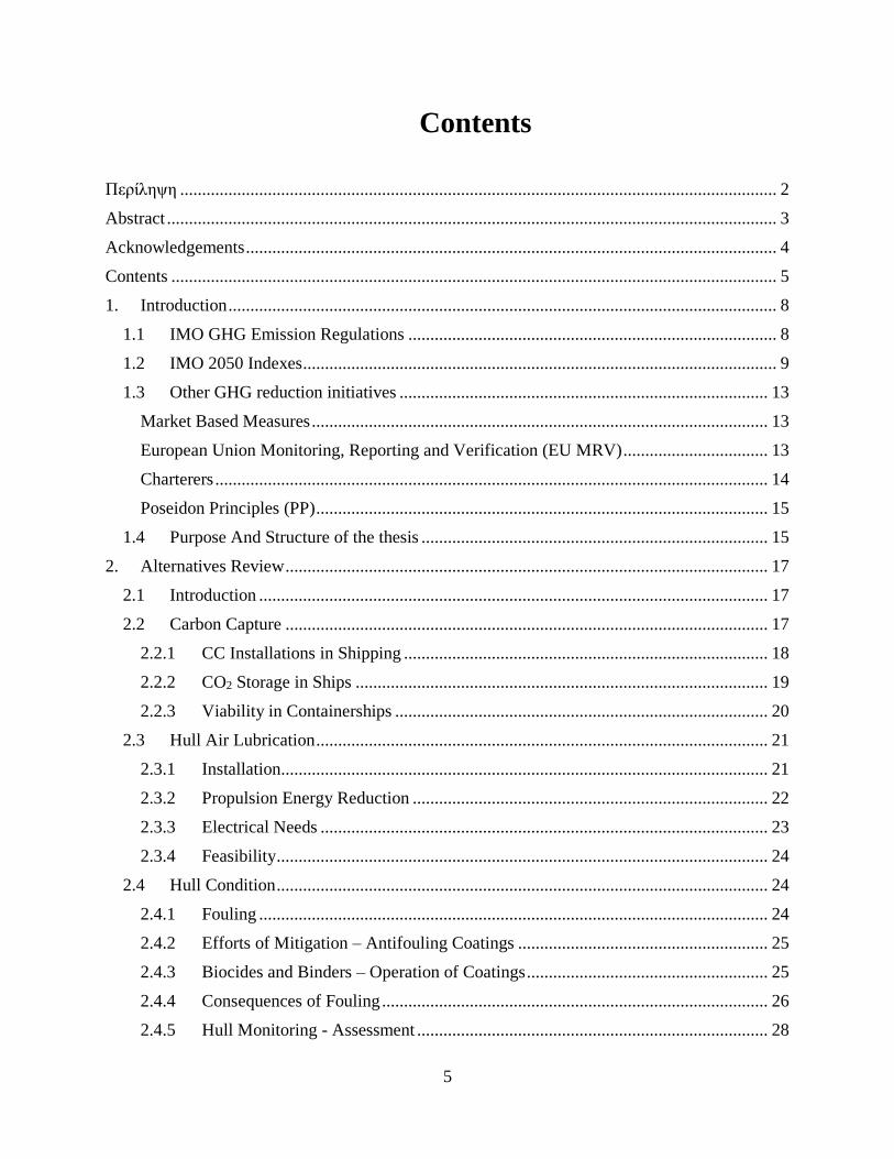
Contents

Περίληψη ........................................................................................................................................ 2

Abstract ........................................................................................................................................... 3

Acknowledgements ......................................................................................................................... 4

Contents .......................................................................................................................................... 5

1. Introduction ............................................................................................................................. 8

1.1 IMO GHG Emission Regulations .................................................................................... 8

1.2 IMO 2050 Indexes ............................................................................................................ 9

1.3 Other GHG reduction initiatives .................................................................................... 13

Market Based Measures ........................................................................................................ 13

European Union Monitoring, Reporting and Verification (EU MRV) ................................. 13

Charterers .............................................................................................................................. 14

Poseidon Principles (PP) ....................................................................................................... 15

1.4 Purpose And Structure of the thesis ............................................................................... 15

2. Alternatives Review .............................................................................................................. 17

2.1 Introduction .................................................................................................................... 17

2.2 Carbon Capture .............................................................................................................. 17

2.2.1 CC Installations in Shipping ................................................................................... 18

2.2.2 CO2 Storage in Ships .............................................................................................. 19

2.2.3 Viability in Containerships ..................................................................................... 20

2.3 Hull Air Lubrication ....................................................................................................... 21

2.3.1 Installation............................................................................................................... 21

2.3.2 Propulsion Energy Reduction ................................................................................. 22

2.3.3 Electrical Needs ...................................................................................................... 23

2.3.4 Feasibility ................................................................................................................ 24

2.4 Hull Condition ................................................................................................................ 24

2.4.1 Fouling .................................................................................................................... 24

2.4.2 Efforts of Mitigation – Antifouling Coatings ......................................................... 25

2.4.3 Biocides and Binders – Operation of Coatings ....................................................... 25

2.4.4 Consequences of Fouling ........................................................................................ 26

2.4.5 Hull Monitoring - Assessment ................................................................................ 28

6

2.5 Trim Optimization .......................................................................................................... 30

2.5.1 Technological Background ..................................................................................... 30

2.5.2 Performance Indexes ............................................................................................... 31

2.5.3 Feasibility ................................................................................................................ 32

2.6 Ballast Water Reduction................................................................................................. 32

2.6.1 Technological Background ..................................................................................... 32

2.6.2 Performance Increase .............................................................................................. 34

2.6.3 Economic assessment.............................................................................................. 34

2.7 Design Speed Optimization ............................................................................................ 35

2.7.1 Technical Considerations ........................................................................................ 36

3.7.2 Market Analysis (Containership Specific) .............................................................. 37

3.7.3 Economic Assessment ............................................................................................ 38

2.8 Weather Routing ............................................................................................................ 38

1. Technological Background ......................................................................................... 38

2. Economic assessment ................................................................................................. 40

2.9 Virtual Arrival ................................................................................................................ 40

2.9.1 Market Analysis - Problems.................................................................................... 40

2.9.2 Technical Background ............................................................................................ 41

2.9.3 Performance Indexes ............................................................................................... 42

2.10 Summary ..................................................................................................................... 42

2.11 Other Alternatives for Compliance with IΜΟ 2050 ................................................... 43

2.11.1 Alternative fuels – Fuel cells .................................................................................. 44

2.11.2 Alternative Power Sources ...................................................................................... 45

2.11.3 Resistance and Propulsion Improvement Methods ................................................. 46

2.11.4 Fuel Efficiency Increase Technologies ................................................................... 47

3. Case Studies – Calculations .................................................................................................. 49

3.1 Introduction .................................................................................................................... 49

3.2 Containers Constructed from Composite Materials ....................................................... 50

3.2.1 Calculations Scope / method ................................................................................... 50

3.2.2 Calculation Process: Composite Containers ........................................................... 50

3.2.3 Examined Ship ........................................................................................................ 52

3.2.4 Resistance Prediction .............................................................................................. 53

3.2.5 Propulsion Prediction .............................................................................................. 60

7

3.2.6 Indexes .................................................................................................................... 69

3.2.7 Economic Analysis ................................................................................................. 72

3.2.8 Results & Comments .............................................................................................. 74

3.3 Super Slow Steaming ..................................................................................................... 75

3.3.1 Calculation Process ................................................................................................. 76

3.3.2 Speed calculation (Resistance & Propulsion) ......................................................... 76

3.3.3 Fuel Consumption / Indexes ................................................................................... 80

3.3.4 Engine Power Limitation ........................................................................................ 83

3.4 Size Optimization – Mega Containerships ..................................................................... 86

3.4.1 Schedules ................................................................................................................ 87

3.4.2 Fuel consumption / Emissions ................................................................................ 90

3.4.3 Economic Analysis ................................................................................................. 91

3.5 Results Summary – Comparison .................................................................................... 93

4. Conclusions – Suggestions for Further Studies .................................................................... 94

5. Citations ................................................................................................................................ 96

6. Index – Additional Information .......................................................................................... 101

6.1 Index A – Carbon Capture Alternatives ....................................................................... 101

6.1.1 Liquid Solvent ....................................................................................................... 101

6.1.2 Solid Sorbents ....................................................................................................... 101

6.1.3 Polymeric Membranes .......................................................................................... 101

6.1.4 Direct Air Capture................................................................................................. 102

6.2 Index B - Future Coatings ............................................................................................ 102

6.2.1 Microtopography Coatings ................................................................................... 102

6.2.2 Shark Skin Imitation Coatings .............................................................................. 102

6.2.3 Climate Change ..................................................................................................... 103

8

1. Introduction

1.1 IMO GHG Emission Regulations

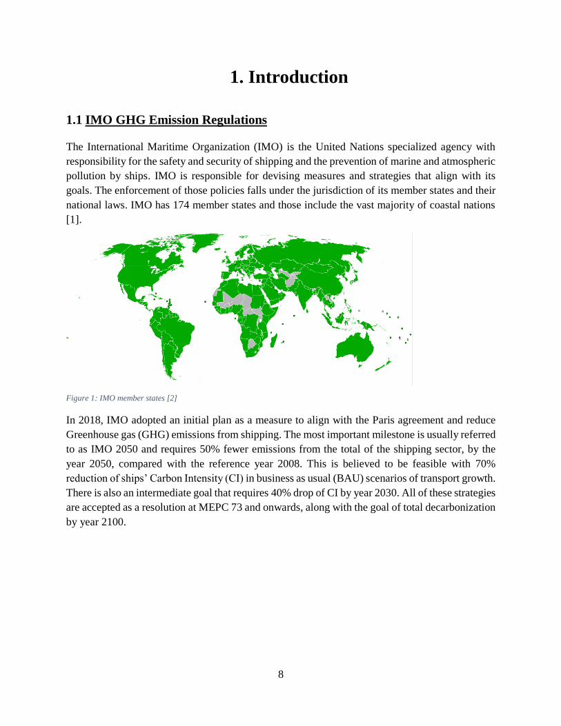
The International Maritime Organization (IMO) is the United Nations specialized agency with

responsibility for the safety and security of shipping and the prevention of marine and atmospheric

pollution by ships. IMO is responsible for devising measures and strategies that align with its

goals. The enforcement of those policies falls under the jurisdiction of its member states and their

national laws. IMO has 174 member states and those include the vast majority of coastal nations

[1].

Figure 1: IMO member states [2]

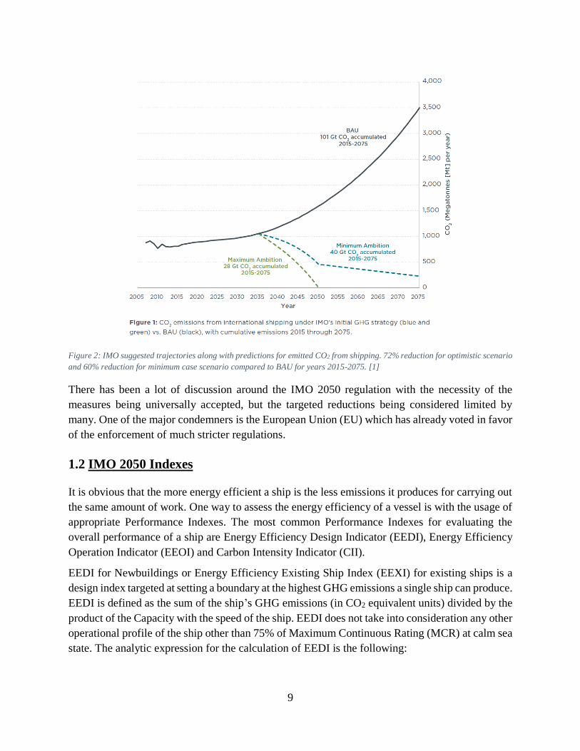
In 2018, IMO adopted an initial plan as a measure to align with the Paris agreement and reduce

Greenhouse gas (GHG) emissions from shipping. The most important milestone is usually referred

to as IMO 2050 and requires 50% fewer emissions from the total of the shipping sector, by the

year 2050, compared with the reference year 2008. This is believed to be feasible with 70%

reduction of ships’ Carbon Intensity (CI) in business as usual (BAU) scenarios of transport growth.

There is also an intermediate goal that requires 40% drop of CI by year 2030. All of these strategies

are accepted as a resolution at MEPC 73 and onwards, along with the goal of total decarbonization

by year 2100.

9

Figure 2: IMO suggested trajectories along with predictions for emitted CO2 from shipping. 72% reduction for optimistic scenario

and 60% reduction for minimum case scenario compared to BAU for years 2015-2075. [1]

There has been a lot of discussion around the IMO 2050 regulation with the necessity of the

measures being universally accepted, but the targeted reductions being considered limited by

many. One of the major condemners is the European Union (EU) which has already voted in favor

of the enforcement of much stricter regulations.

1.2 IMO 2050 Indexes

It is obvious that the more energy efficient a ship is the less emissions it produces for carrying out

the same amount of work. One way to assess the energy efficiency of a vessel is with the usage of

appropriate Performance Indexes. The most common Performance Indexes for evaluating the

overall performance of a ship are Energy Efficiency Design Indicator (EEDI), Energy Efficiency

Operation Indicator (EEOI) and Carbon Intensity Indicator (CII).

EEDI for Newbuildings or Energy Efficiency Existing Ship Index (EEXI) for existing ships is a

design index targeted at setting a boundary at the highest GHG emissions a single ship can produce.

EEDI is defined as the sum of the ship’s GHG emissions (in CO2 equivalent units) divided by the

product of the Capacity with the speed of the ship. EEDI does not take into consideration any other

operational profile of the ship other than 75% of Maximum Continuous Rating (MCR) at calm sea

state. The analytic expression for the calculation of EEDI is the following:

10

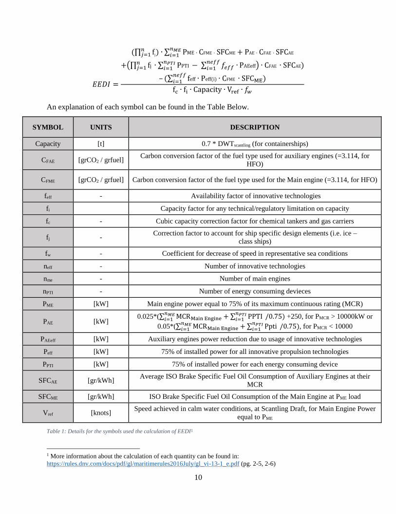
𝐸𝐸𝐷𝐼 =

(∏ fj) ∙ ∑ PME ∙ CFME ∙ SFCME𝑛𝑀𝐸𝑖=1

𝑛𝑗=1 + PAE ∙ CFAE ∙ SFCAE

+(∏ fj ∙ ∑ PPTI − ∑ 𝑓𝑒𝑓𝑓 ∙𝑛𝑒𝑓𝑓𝑖=1

𝑛𝑃𝑇𝐼𝑖=1 PAEeff𝑛

𝑗=1 ) ∙ CFAE ∙ SFCAE)

– (∑ feff ∙ Peff(i) ∙ CFME ∙ SFCME𝑛𝑒𝑓𝑓𝑖=1 )

fc ∙ fi ∙ Capacity ∙ Vref ∙ 𝑓𝑤

An explanation of each symbol can be found in the Table Below.

SYMBOL UNITS DESCRIPTION

Capacity [t] 0.7 * DWTscantling (for containerships)

CFAE [grCO2 / grfuel] Carbon conversion factor of the fuel type used for auxiliary engines (=3.114, for

HFO)

CFME [grCO2 / grfuel] Carbon conversion factor of the fuel type used for the Main engine (=3.114, for HFO)

feff - Availability factor of innovative technologies

fi Capacity factor for any technical/regulatory limitation on capacity

fc - Cubic capacity correction factor for chemical tankers and gas carriers

fj - Correction factor to account for ship specific design elements (i.e. ice –

class ships)

fw - Coefficient for decrease of speed in representative sea conditions

neff - Number of innovative technologies

nme - Number of main engines

nPTI - Number of energy consuming devieces

PME [kW] Main engine power equal to 75% of its maximum continuous rating (MCR)

PAE [kW] 0.025*(∑ MCRMain Engine + ∑ PPTI

𝑛𝑃𝑇𝐼𝑖=1 /0.75)

𝑛𝑀𝐸𝑖=1 +250, for PMCR > 10000kW or

0.05*(∑ MCRMain Engine + ∑ Ppti 𝑛𝑃𝑇𝐼𝑖=1 /0.75)

𝑛𝑀𝐸𝑖=1 , for PMCR < 10000

PAEeff [kW] Auxiliary engines power reduction due to usage of innovative technologies

Peff [kW] 75% of installed power for all innovative propulsion technologies

PPTI [kW] 75% of installed power for each energy consuming device

SFCAE [gr/kWh] Average ISO Brake Specific Fuel Oil Consumption of Auxiliary Engines at their

MCR

SFCME [gr/kWh] ISO Brake Specific Fuel Oil Consumption of the Main Engine at PME load

Vref [knots] Speed achieved in calm water conditions, at Scantling Draft, for Main Engine Power

equal to PME

Table 1: Details for the symbols used the calculation of EEDI1

1 More information about the calculation of each quantity can be found in:

https://rules.dnv.com/docs/pdf/gl/maritimerules2016July/gl_vi-13-1_e.pdf (pg. 2-5, 2-6)

11

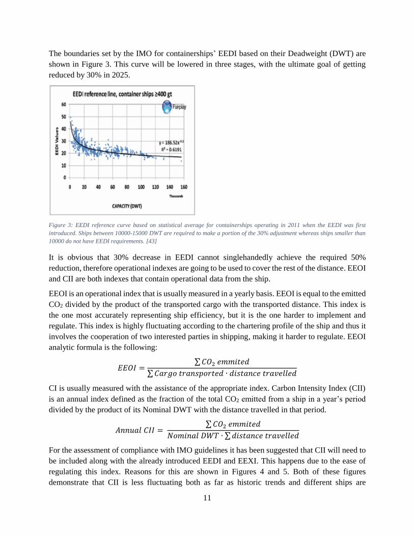
The boundaries set by the IMO for containerships’ EEDI based on their Deadweight (DWT) are

shown in Figure 3. This curve will be lowered in three stages, with the ultimate goal of getting

reduced by 30% in 2025.

Figure 3: EEDI reference curve based on statistical average for containerships operating in 2011 when the EEDI was first

introduced. Ships between 10000-15000 DWT are required to make a portion of the 30% adjustment whereas ships smaller than

10000 do not have EEDI requirements. [43]

It is obvious that 30% decrease in EEDI cannot singlehandedly achieve the required 50%

reduction, therefore operational indexes are going to be used to cover the rest of the distance. EEOI

and CII are both indexes that contain operational data from the ship.

EEOI is an operational index that is usually measured in a yearly basis. EEOI is equal to the emitted

CO2 divided by the product of the transported cargo with the transported distance. This index is

the one most accurately representing ship efficiency, but it is the one harder to implement and

regulate. This index is highly fluctuating according to the chartering profile of the ship and thus it

involves the cooperation of two interested parties in shipping, making it harder to regulate. EEOI

analytic formula is the following:

𝐸𝐸𝑂𝐼 =∑𝐶𝑂2 𝑒𝑚𝑚𝑖𝑡𝑒𝑑

∑𝐶𝑎𝑟𝑔𝑜 𝑡𝑟𝑎𝑛𝑠𝑝𝑜𝑟𝑡𝑒𝑑 ∙ 𝑑𝑖𝑠𝑡𝑎𝑛𝑐𝑒 𝑡𝑟𝑎𝑣𝑒𝑙𝑙𝑒𝑑

CI is usually measured with the assistance of the appropriate index. Carbon Intensity Index (CII)

is an annual index defined as the fraction of the total CO2 emitted from a ship in a year’s period

divided by the product of its Nominal DWT with the distance travelled in that period.

𝐴𝑛𝑛𝑢𝑎𝑙 𝐶𝐼𝐼 = ∑𝐶𝑂2 𝑒𝑚𝑚𝑖𝑡𝑒𝑑

𝑁𝑜𝑚𝑖𝑛𝑎𝑙 𝐷𝑊𝑇 ∙ ∑𝑑𝑖𝑠𝑡𝑎𝑛𝑐𝑒 𝑡𝑟𝑎𝑣𝑒𝑙𝑙𝑒𝑑

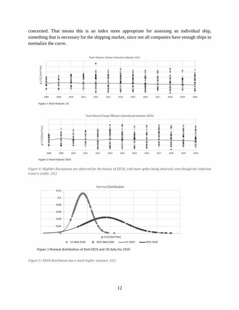
For the assessment of compliance with IMO guidelines it has been suggested that CII will need to

be included along with the already introduced EEDI and EEXI. This happens due to the ease of

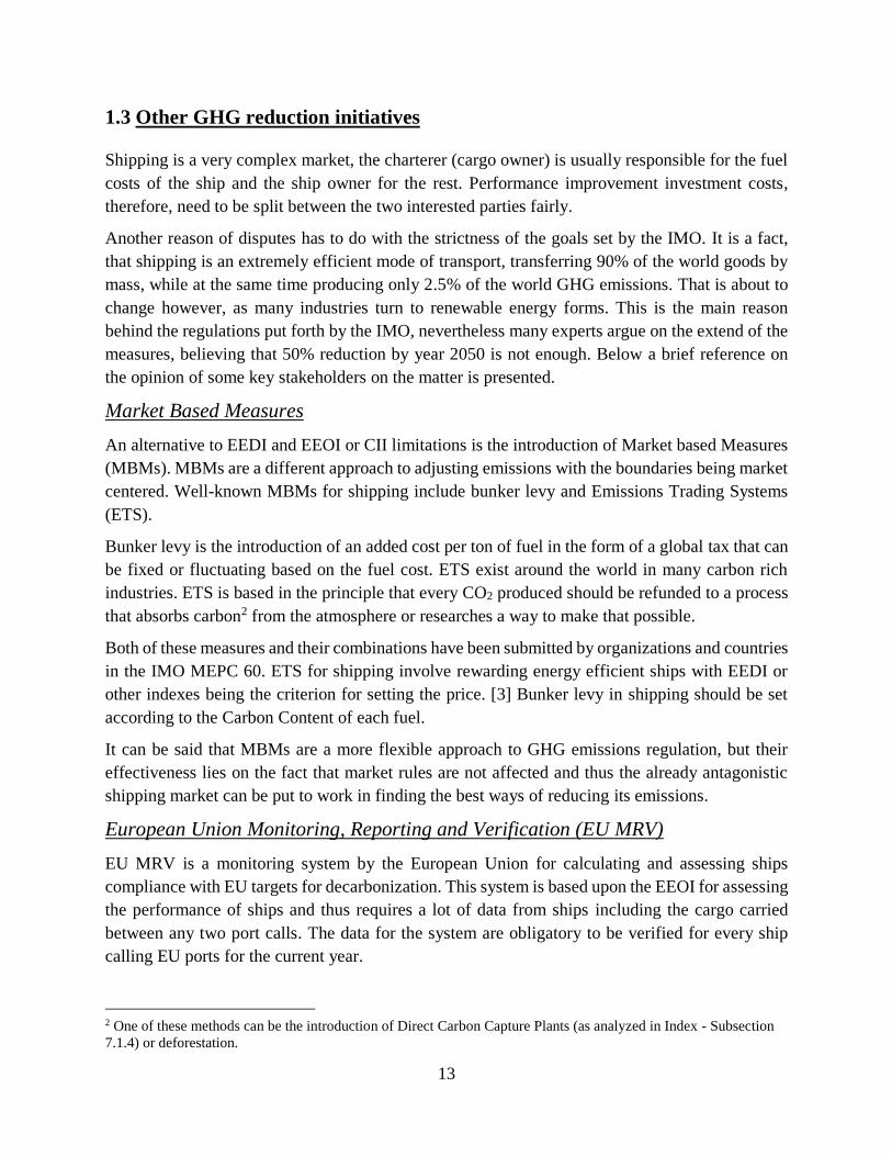
regulating this index. Reasons for this are shown in Figures 4 and 5. Both of these figures

demonstrate that CII is less fluctuating both as far as historic trends and different ships are

12

concerned. That means this is an index more appropriate for assessing an individual ship,

something that is necessary for the shipping market, since not all companies have enough ships to

normalize the curve.

Figure 4: HighΒer fluctuations are observed for the history of EEOI, with more spikes being observed, even though the reduction

trend is visible. [41]

Figure 5: EEOI distribution has a much higher variance. [41]

13

1.3 Other GHG reduction initiatives

Shipping is a very complex market, the charterer (cargo owner) is usually responsible for the fuel

costs of the ship and the ship owner for the rest. Performance improvement investment costs,

therefore, need to be split between the two interested parties fairly.

Another reason of disputes has to do with the strictness of the goals set by the IMO. It is a fact,

that shipping is an extremely efficient mode of transport, transferring 90% of the world goods by

mass, while at the same time producing only 2.5% of the world GHG emissions. That is about to

change however, as many industries turn to renewable energy forms. This is the main reason

behind the regulations put forth by the IMO, nevertheless many experts argue on the extend of the

measures, believing that 50% reduction by year 2050 is not enough. Below a brief reference on

the opinion of some key stakeholders on the matter is presented.

Market Based Measures

An alternative to EEDI and EEOI or CII limitations is the introduction of Market based Measures

(MBMs). MBMs are a different approach to adjusting emissions with the boundaries being market

centered. Well-known MBMs for shipping include bunker levy and Emissions Trading Systems

(ETS).

Bunker levy is the introduction of an added cost per ton of fuel in the form of a global tax that can

be fixed or fluctuating based on the fuel cost. ETS exist around the world in many carbon rich

industries. ETS is based in the principle that every CO2 produced should be refunded to a process

that absorbs carbon2 from the atmosphere or researches a way to make that possible.

Both of these measures and their combinations have been submitted by organizations and countries

in the IMO MEPC 60. ETS for shipping involve rewarding energy efficient ships with EEDI or

other indexes being the criterion for setting the price. [3] Bunker levy in shipping should be set

according to the Carbon Content of each fuel.

It can be said that MBMs are a more flexible approach to GHG emissions regulation, but their

effectiveness lies on the fact that market rules are not affected and thus the already antagonistic

shipping market can be put to work in finding the best ways of reducing its emissions.

European Union Monitoring, Reporting and Verification (EU MRV)

EU MRV is a monitoring system by the European Union for calculating and assessing ships

compliance with EU targets for decarbonization. This system is based upon the EEOI for assessing

the performance of ships and thus requires a lot of data from ships including the cargo carried

between any two port calls. The data for the system are obligatory to be verified for every ship

calling EU ports for the current year.

2 One of these methods can be the introduction of Direct Carbon Capture Plants (as analyzed in Index - Subsection

7.1.4) or deforestation.

14

EU is planning to introduce EU MRV to the EU Emissions Trading System (EU ETS), with ships

calling EU ports being subject to additional costs proportional to their emissions. The target set by

the EU is 90% reduction for transport emissions by 2050 and so far no additional regulation has

been put forth for the shipping market. Another difference with IMO regulation is the fact that EU

imposes bans on the shipping firm’s total, whereas the IMO forces a company to scrap only one

of its ships when compliance is not met. [44], [45]

Charterers

Charterers define shipping business in many ways as their demands are the ones that need to be

met. Charterers of the shipping business can be oil companies, steel industry companies or even

other shipping companies. In the container shipping business, the charter is usually another

shipping company since the transferred package is by definition reduced. Many container shipping

companies – charters have already set an extremely ambitious decarbonization trajectories. One of

those is the leader of the containership market as of this moment, A.P. Moller – Maersk, that aims

to achieve total decarbonization by year 2050.

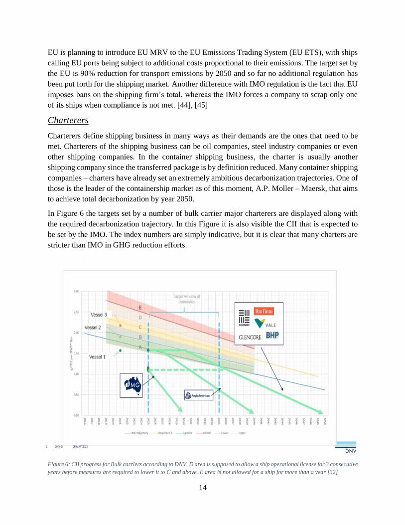
In Figure 6 the targets set by a number of bulk carrier major charterers are displayed along with

the required decarbonization trajectory. In this Figure it is also visible the CII that is expected to

be set by the IMO. The index numbers are simply indicative, but it is clear that many charters are

stricter than IMO in GHG reduction efforts.

Figure 6: CII progress for Bulk carriers according to DNV. D area is supposed to allow a ship operational license for 3 consecutive

years before measures are required to lower it to C and above. E area is not allowed for a ship for more than a year [32]

15

Poseidon Principles (PP)

Another aspect of dealing with emissions is by affecting the funding of shipping companies. One

such initiative has been taken by 27 leading banks, jointly representing approximately USD 185

billion of shipping finance in PP. [42] PP is an agreement with the target of assisting in the efforts

to meet IMO 2050 targets. The operational framework of PP relies on the promotion of assessment,

accountability, enforcement and transparency practices in the evaluation of investments in

shipping.

The scope of PP is alignment with IMO absolute target of 50% reduction. In order to perform this

an index equivalent to CII called Annual Efficiency Ratio (AER) is used. This index is updated

yearly, starting from year 2012to match a linear path to 50% reduction of emissions compared to

reference year 2008. The evaluation of each financial institution is done by summing up all its

loans multiplied by the misalignment percentage with AER required for the reference year. Results

for each signatory after being evaluated are disclosed whereas each signatory is committed to

making its best effort to improve its score.

1.4 Purpose And Structure of the thesis

This diploma thesis examines the options available for containerships to reduce GHG emissions

in order to be compliant with IMO 2050 regulations. The main concern throughout this thesis is

the GHG emissions reduction potential of each alternative. Secondly, economic impact of each

alternative is addressed when necessary data are available. Many alternatives are not market

available options and therefore, emission reduction potential was extracted from predictions. This

thesis overall is not concerned with operational data as IMO 2050 goals are very ambitious and

most methods to make these targets a reality are not yet tested.

The target of this thesis is to make predictions concerning measures of GHG reduction and evaluate

them according to their effectiveness. Structural and other construction issues are not addressed.

The analysis of this thesis is broken down in two Parts, Chapters 3 and 4 respectively.

Chapter 3 is concerned with the analysis of numerus alternatives that are particularly applicable to

containerships. Chapter 3 aims mainly at presenting available alternatives based on bibliography

so as to demonstrate the effect on containerships.

Chapter 4 contains three case studies for containerships: composite containers, super slow

steaming and Size Utilization. All of these cases are analyzed with respect to extracting data for

consumption and translating that to appropriate indexes for evaluation. Data have been acquired

from actual ships in both of the case studies. This Chapter is mainly focused at evaluating available

alternatives and could serve as a guideline for further evaluations.

Throughout Chapters 3 and 4 all alternatives analyzed will take into consideration only GHG

emissions from ship operation. Emissions resulting from Shipbuilding, Dry Docking and other

maintenance operations if not else stated will not be analyzed. Furthermore, Particulate Matter

16

(PM), Nitrogen Oxides (NOx) and other emissions will not be taken into consideration when

analyzing the impact of each alternative. Finally, health and safety of workers and marine hazards

(fire, loss of stability, etc.), if not mentioned are not concerning this Thesis.

Finally, conclusions have been drawn with respect to utility of the analyzed alternatives along with

suggestions for further studies. All the alternatives are discussed under the scope of the impact in

emissions from being implemented in future and existing ships.

17

2. Alternatives Review

2.1 Introduction

As already mentioned the necessary target indexes for meeting IMO targets for GHG reduction

are not yet explicit. It is a fact nevertheless, that ships will need to be more environmentally

friendly. A measure towards that direction is the application of a number of alternatives that

increase the energy efficiency of ships. A number of these alternatives will be analyzed in detail

below and a few more will be briefly mentioned in Section 3.10. IMO targets specify an initial

step requiring 40% decrease in consumption per transported cargo and another 70% followed

shortly. Most of the alternatives below have the potential to achieve part of this decrease (excluding

Carbon Capture) and as a result it is almost certain that more than one will need to be implemented

in every ship.

2.2 Carbon Capture

Carbon Capture (CC) has been a relevantly new method of lowering GHG emissions. As of 2019

there were 17 CC facilities around the world in operation, but that number has been constantly

increasing and the momentum this method has seen in land could makes this a very interesting

option for the shipping sector.

CC is the most effective method of reducing GHG emissions from shipping and has the potential

of singlehandedly offering up to 90% reduction in CO2 emissions. [8] The idea behind CC is

relatively simple, but the technology required to operate a CC system efficiently is advanced. CC

works by removing the CO2 from the exhaust gases of a ship and storing them for discharge on

shore or at sea drop sites3. The difficulty lies in both filtering out the CO2 particles and storing

them safely and efficiently until the next port.

CC works in a similar principle as the much discussed SOx scrubbers. The main idea is to force

exhaust gases through a filter which separates CO2 and then transform it in a form (liquid or

supercritical fluid state) that can be stored on board or disposed in the sea. The idea is simple, but

the ways to incorporate it can vary.

There are three industry used methods to separate CO2 from exhaust gasses. Each of them performs

a different procedure to filter out the CO2 and has its own advantages and drawbacks. The main

difference is found in the material used in the separation. The three alternatives are based on: a

liquid solvent, a solid sorbent and a polymeric membrane. All of these processes and the associated

advantages and disadvantages are discussed in detail in the Index A – Section 7.1.

3 CO2 drop sites can be either at Sea Depths of more than 2500m or at emptied or partially emptied Oil Mines (as

fluid for fracking – this method is not carbon neutral).

18

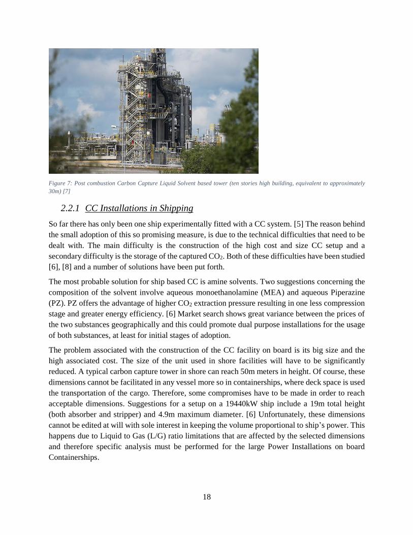
Figure 7: Post combustion Carbon Capture Liquid Solvent based tower (ten stories high building, equivalent to approximately

30m) [7]

2.2.1 CC Installations in Shipping

So far there has only been one ship experimentally fitted with a CC system. [5] The reason behind

the small adoption of this so promising measure, is due to the technical difficulties that need to be

dealt with. The main difficulty is the construction of the high cost and size CC setup and a

secondary difficulty is the storage of the captured CO2. Both of these difficulties have been studied

[6], [8] and a number of solutions have been put forth.

The most probable solution for ship based CC is amine solvents. Two suggestions concerning the

composition of the solvent involve aqueous monoethanolamine (MEA) and aqueous Piperazine

(PZ). PZ offers the advantage of higher CO2 extraction pressure resulting in one less compression

stage and greater energy efficiency. [6] Market search shows great variance between the prices of

the two substances geographically and this could promote dual purpose installations for the usage

of both substances, at least for initial stages of adoption.

The problem associated with the construction of the CC facility on board is its big size and the

high associated cost. The size of the unit used in shore facilities will have to be significantly

reduced. A typical carbon capture tower in shore can reach 50m meters in height. Of course, these

dimensions cannot be facilitated in any vessel more so in containerships, where deck space is used

the transportation of the cargo. Therefore, some compromises have to be made in order to reach

acceptable dimensions. Suggestions for a setup on a 19440kW ship include a 19m total height

(both absorber and stripper) and 4.9m maximum diameter. [6] Unfortunately, these dimensions

cannot be edited at will with sole interest in keeping the volume proportional to ship’s power. This

happens due to Liquid to Gas (L/G) ratio limitations that are affected by the selected dimensions

and therefore specific analysis must be performed for the large Power Installations on board

Containerships.

19

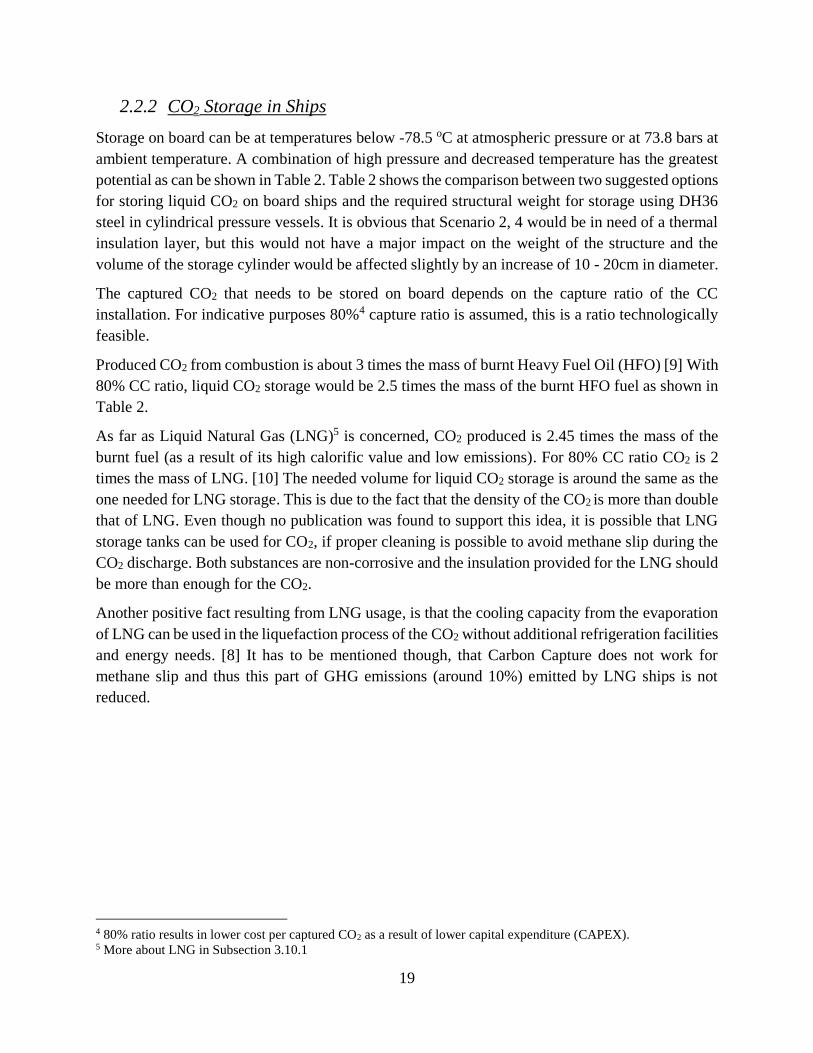
2.2.2 CO2 Storage in Ships

Storage on board can be at temperatures below -78.5 oC at atmospheric pressure or at 73.8 bars at

ambient temperature. A combination of high pressure and decreased temperature has the greatest

potential as can be shown in Table 2. Table 2 shows the comparison between two suggested options

for storing liquid CO2 on board ships and the required structural weight for storage using DH36

steel in cylindrical pressure vessels. It is obvious that Scenario 2, 4 would be in need of a thermal

insulation layer, but this would not have a major impact on the weight of the structure and the

volume of the storage cylinder would be affected slightly by an increase of 10 - 20cm in diameter.

The captured CO2 that needs to be stored on board depends on the capture ratio of the CC

installation. For indicative purposes 80%4 capture ratio is assumed, this is a ratio technologically

feasible.

Produced CO2 from combustion is about 3 times the mass of burnt Heavy Fuel Oil (HFO) [9] With

80% CC ratio, liquid CO2 storage would be 2.5 times the mass of the burnt HFO fuel as shown in

Table 2.

As far as Liquid Natural Gas (LNG)5 is concerned, CO2 produced is 2.45 times the mass of the

burnt fuel (as a result of its high calorific value and low emissions). For 80% CC ratio CO2 is 2

times the mass of LNG. [10] The needed volume for liquid CO2 storage is around the same as the

one needed for LNG storage. This is due to the fact that the density of the CO2 is more than double

that of LNG. Even though no publication was found to support this idea, it is possible that LNG

storage tanks can be used for CO2, if proper cleaning is possible to avoid methane slip during the

CO2 discharge. Both substances are non-corrosive and the insulation provided for the LNG should

be more than enough for the CO2.

Another positive fact resulting from LNG usage, is that the cooling capacity from the evaporation

of LNG can be used in the liquefaction process of the CO2 without additional refrigeration facilities

and energy needs. [8] It has to be mentioned though, that Carbon Capture does not work for

methane slip and thus this part of GHG emissions (around 10%) emitted by LNG ships is not

reduced.

4 80% ratio results in lower cost per captured CO2 as a result of lower capital expenditure (CAPEX). 5 More about LNG in Subsection 3.10.1

20

Scenario 1 Scenario 2 Scenario 3 Scenario 4

p (bar) 100 11 100 11

T (oC) 35 -50 35 -50

CO2 Density (kg/m3) 700 1150 700 1150

Fuel Used HFO HFO LNG LNG

Fuel Density (kg/m3) 1000 1000 450 450

CC ratio 80% 80% 80% 80%

Outer Diameter -

without insulation- (m) 10 10 10 10

CO2 Mass (t) 366.5 602.1 366.5 602.1

Total Volume (m3) 553.9 526.9 553.9 526.9

σallowable - AH36 (MPa) 264 264 264 264

shell thickness, t (m) 0.1894 0.0208 0.1894 0.0208

Added weight due to

steel structure (kg) 236472.08 25578.66 236472.08 25578.66

Steel Structure to CO2

weight ratio 64.52% 4.25% 64.52% 4.25%

Total Volume to CO2

mass ratio (m3/t) 1.511 0.875 1.511 0.875

Burnt Fuel to captured

CO2 mass ratio 2.400 2.400 1.960 1.960

Burnt Fuel to captured

CO2 volumetric ratio 3.429 2.087 1.260 0.767

Added fuel Cost ($/ton) 221.340 221.340 180.761 180.761

Table 2: Comparison between suggested options for Captured CO2 storage found in [6], [8]. Analysis for both HFO and LNG.

2.2.3 Viability in Containerships

Containerships could be at an advantageous position as far as storage is concerned, taking

advantage of their often port calls to unload liquid CO2 tanks. All in all, if CC was to be

implemented in a containership fueled by LNG it is not very ambitious to expect prices lower than

the optimistic 77.5 €/ton CO2. That is due to economies of scale on the CAPEX of the CC facility

(around €35 million for 19440kW ship) that is almost 70% of the total cost. [6]

21

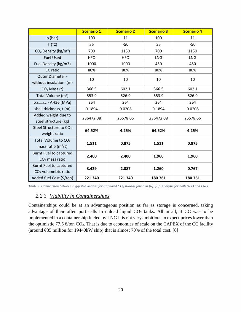
2.3 Hull Air Lubrication

Hull air Lubrication systems (ALS) is a recently introduced method for reducing frictional

resistance of ships. This method works by injecting air in the bottom part of the ship and creating

a boundary layer that drags the ships bottom in air. The way this method works is by exploiting

the principle that air density is smaller than water, therefore smaller frictional resistance is

occurring. The problem with this method lies in keeping the air layer intact.

A containership covers its full length in travelling distance in 20 to 60 seconds depending on its

cruising speed and dimensions. What is more, moving objects, under the effect of waves,

experience rotations and movements in multiple axis. The effort of keeping a fluid of decreased

density from rising to the surface for the required time is made a lot harder under the effect of such

motions.

ALS has seen a number of installations in the past years with many more planned for the years

ahead. [58]

Figure 8: Hull air lubrication with microbubbles. Illustration of design by Silverstream®. Savings of 5-10% are expected from

such a solution. [54]

2.3.1 Installation

There are three main types of hull air lubrication installations, each having associated advantages

and drawbacks. The main difference is in the method of confining the air below the hull.

Air lubrication using an air film was the first form of air lubrication used. This method uses a

constant flow of air in the ships Flat of Bottom (FOB) are in order to create a film of adequate

thickness for the ship to experience reduced frictional resistance. The advantages of this method

is the ability to retrofit in existing vessels, the high reduction of frictional resistance and the small

22

effect on shipping maneuvering characteristics. The drawbacks associated with air film include

high airflow to maintain the required layer, and limitations as far as length is concerned.

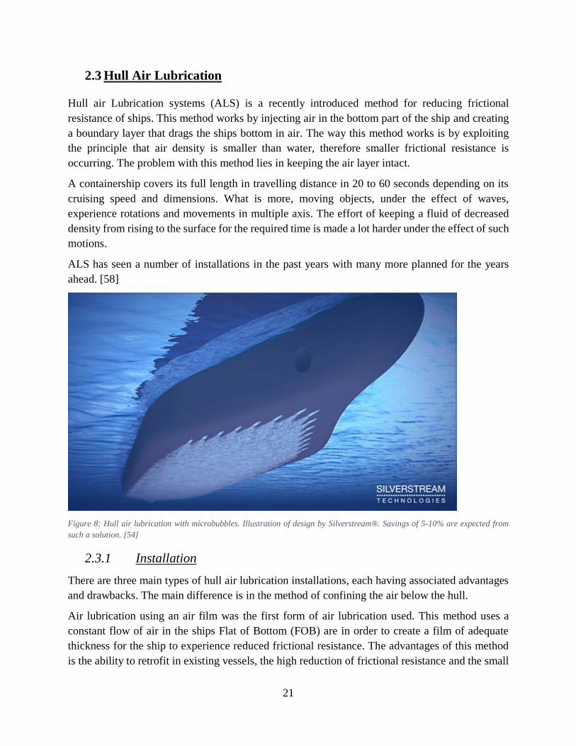
Air Cavities is a very efficient method of air lubrication. This method uses the same principle as

air film, but the FOB area is confined in order to minimize the outflow of air. This method by

design requires reduced airflow rate, and thus has smaller compressors and energy needs. What is

more, the area of effect is the largest one possible limited only by the FOB. The problems with

this method are the inability to retrofit existing ships and the loss of effectiveness when the ship is

rotating under the effect of large waves.

Figure 9: SSPA investigated different designs for the project P-MAX air to minimize the resistance of the 182m tanker. Photo:

Courtesy of STENA AB. Read more at www.sspa.se. Air Cavity Illustration [55]

Air lubrication using microbubbles is the most used retrofitting option for existing ships. This

method is an evolution of the air film method injecting air in the form of bubbles in the FOB area

of the ship. This way less compressed air is needed. Problems with this method include bubbles

size propagation that results in loss of adherence to the boundary layer and small length of effect

requiring multiple injectors across the ships bottom on large ships.

2.3.2 Propulsion Energy Reduction

Propulsion Power reduction for each method is highly dependent on the Sea Condition the ship

operates and the FOB area characteristics. The greatest reductions are expected for ships with

increased FOB to Wetted Surface Area (WSA) ratios sailing in calm waters.

Unfortunately, containerships have reduced FOB areas due to their slenderness. FOB to WSA ratio

is 20% for a 4250 TEU containership, whereas the same ratio can reach values up to 40% for a

Very Large Crude Oil Carrier (VLCC).

23

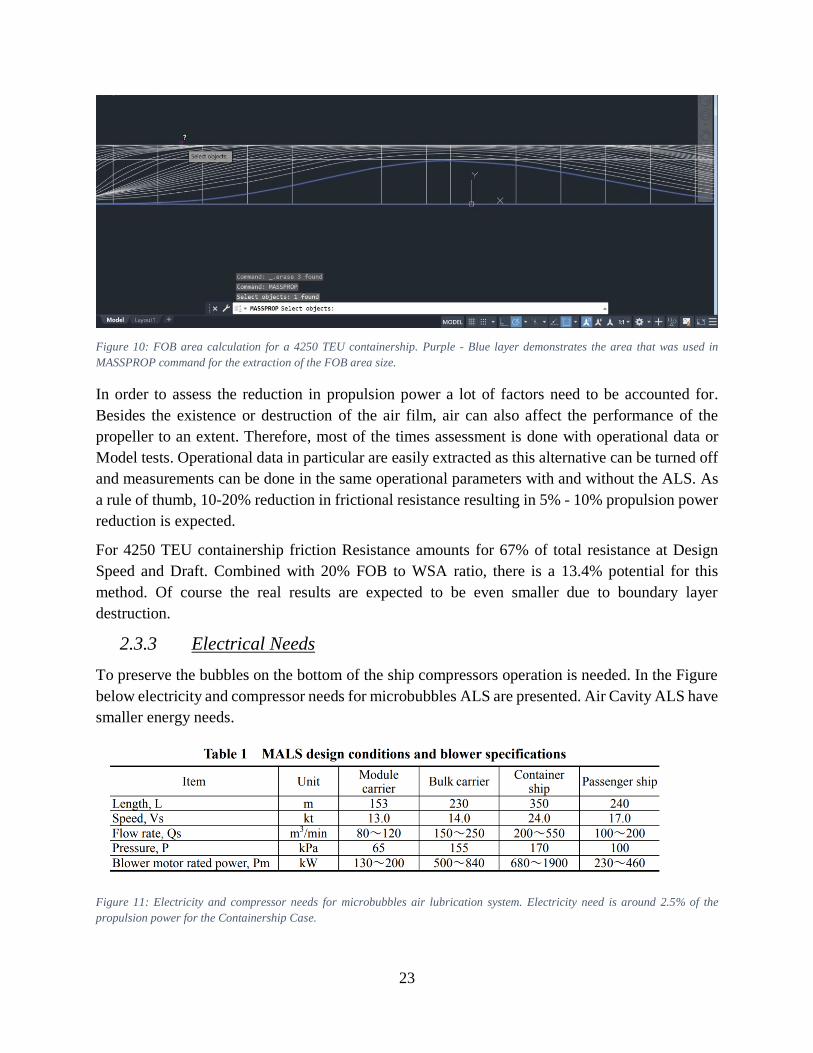
Figure 10: FOB area calculation for a 4250 TEU containership. Purple - Blue layer demonstrates the area that was used in

MASSPROP command for the extraction of the FOB area size.

In order to assess the reduction in propulsion power a lot of factors need to be accounted for.

Besides the existence or destruction of the air film, air can also affect the performance of the

propeller to an extent. Therefore, most of the times assessment is done with operational data or

Model tests. Operational data in particular are easily extracted as this alternative can be turned off

and measurements can be done in the same operational parameters with and without the ALS. As

a rule of thumb, 10-20% reduction in frictional resistance resulting in 5% - 10% propulsion power

reduction is expected.

For 4250 TEU containership friction Resistance amounts for 67% of total resistance at Design

Speed and Draft. Combined with 20% FOB to WSA ratio, there is a 13.4% potential for this

method. Of course the real results are expected to be even smaller due to boundary layer

destruction.

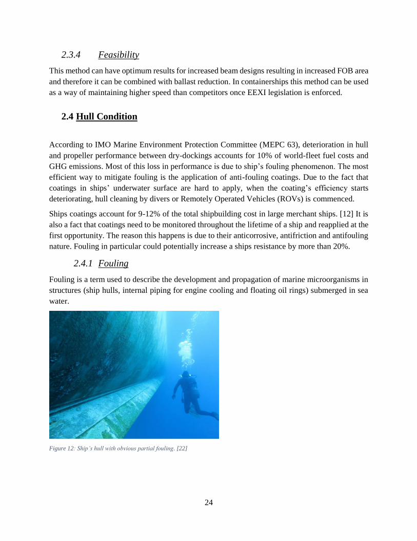
2.3.3 Electrical Needs

To preserve the bubbles on the bottom of the ship compressors operation is needed. In the Figure

below electricity and compressor needs for microbubbles ALS are presented. Air Cavity ALS have

smaller energy needs.

Figure 11: Electricity and compressor needs for microbubbles air lubrication system. Electricity need is around 2.5% of the

propulsion power for the Containership Case.

24

2.3.4 Feasibility

This method can have optimum results for increased beam designs resulting in increased FOB area

and therefore it can be combined with ballast reduction. In containerships this method can be used

as a way of maintaining higher speed than competitors once EEXI legislation is enforced.

2.4 Hull Condition

According to IMO Marine Environment Protection Committee (MEPC 63), deterioration in hull

and propeller performance between dry-dockings accounts for 10% of world-fleet fuel costs and

GHG emissions. Most of this loss in performance is due to ship’s fouling phenomenon. The most

efficient way to mitigate fouling is the application of anti-fouling coatings. Due to the fact that

coatings in ships’ underwater surface are hard to apply, when the coating’s efficiency starts

deteriorating, hull cleaning by divers or Remotely Operated Vehicles (ROVs) is commenced.

Ships coatings account for 9-12% of the total shipbuilding cost in large merchant ships. [12] It is

also a fact that coatings need to be monitored throughout the lifetime of a ship and reapplied at the

first opportunity. The reason this happens is due to their anticorrosive, antifriction and antifouling

nature. Fouling in particular could potentially increase a ships resistance by more than 20%.

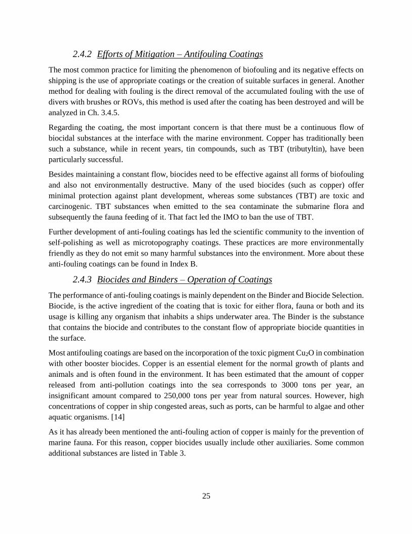
2.4.1 Fouling

Fouling is a term used to describe the development and propagation of marine microorganisms in

structures (ship hulls, internal piping for engine cooling and floating oil rings) submerged in sea

water.

Figure 12: Ship’s hull with obvious partial fouling. [22]

25

2.4.2 Efforts of Mitigation – Antifouling Coatings

The most common practice for limiting the phenomenon of biofouling and its negative effects on

shipping is the use of appropriate coatings or the creation of suitable surfaces in general. Another

method for dealing with fouling is the direct removal of the accumulated fouling with the use of

divers with brushes or ROVs, this method is used after the coating has been destroyed and will be

analyzed in Ch. 3.4.5.

Regarding the coating, the most important concern is that there must be a continuous flow of

biocidal substances at the interface with the marine environment. Copper has traditionally been

such a substance, while in recent years, tin compounds, such as TBT (tributyltin), have been

particularly successful.

Besides maintaining a constant flow, biocides need to be effective against all forms of biofouling

and also not environmentally destructive. Many of the used biocides (such as copper) offer

minimal protection against plant development, whereas some substances (TBT) are toxic and

carcinogenic. TBT substances when emitted to the sea contaminate the submarine flora and

subsequently the fauna feeding of it. That fact led the IMO to ban the use of TBT.

Further development of anti-fouling coatings has led the scientific community to the invention of

self-polishing as well as microtopography coatings. These practices are more environmentally

friendly as they do not emit so many harmful substances into the environment. More about these

anti-fouling coatings can be found in Index B.

2.4.3 Biocides and Binders – Operation of Coatings

The performance of anti-fouling coatings is mainly dependent on the Binder and Biocide Selection.

Biocide, is the active ingredient of the coating that is toxic for either flora, fauna or both and its

usage is killing any organism that inhabits a ships underwater area. The Binder is the substance

that contains the biocide and contributes to the constant flow of appropriate biocide quantities in

the surface.

Most antifouling coatings are based on the incorporation of the toxic pigment Cu2O in combination

with other booster biocides. Copper is an essential element for the normal growth of plants and

animals and is often found in the environment. It has been estimated that the amount of copper

released from anti-pollution coatings into the sea corresponds to 3000 tons per year, an

insignificant amount compared to 250,000 tons per year from natural sources. However, high

concentrations of copper in ship congested areas, such as ports, can be harmful to algae and other

aquatic organisms. [14]

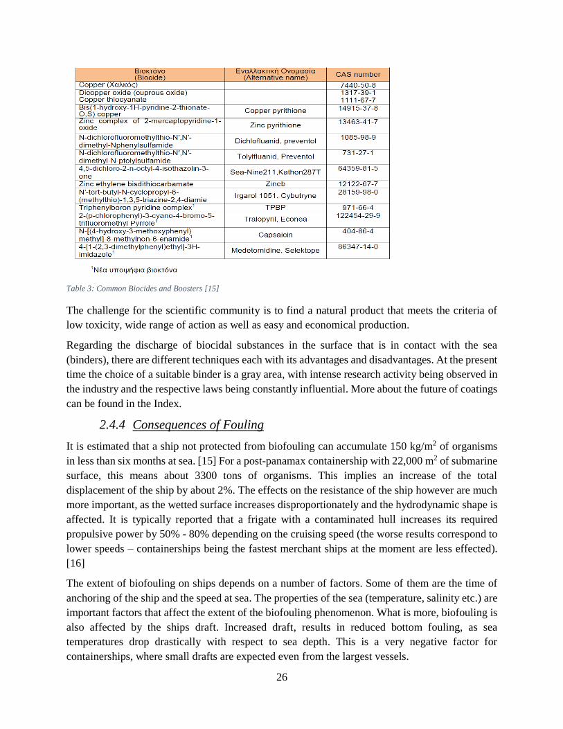
As it has already been mentioned the anti-fouling action of copper is mainly for the prevention of

marine fauna. For this reason, copper biocides usually include other auxiliaries. Some common

additional substances are listed in Table 3.

26

Table 3: Common Biocides and Boosters [15]

The challenge for the scientific community is to find a natural product that meets the criteria of

low toxicity, wide range of action as well as easy and economical production.

Regarding the discharge of biocidal substances in the surface that is in contact with the sea

(binders), there are different techniques each with its advantages and disadvantages. At the present

time the choice of a suitable binder is a gray area, with intense research activity being observed in

the industry and the respective laws being constantly influential. More about the future of coatings

can be found in the Index.

2.4.4 Consequences of Fouling

It is estimated that a ship not protected from biofouling can accumulate 150 kg/m2 of organisms

in less than six months at sea. [15] For a post-panamax containership with 22,000 m2 of submarine

surface, this means about 3300 tons of organisms. This implies an increase of the total

displacement of the ship by about 2%. The effects on the resistance of the ship however are much

more important, as the wetted surface increases disproportionately and the hydrodynamic shape is

affected. It is typically reported that a frigate with a contaminated hull increases its required

propulsive power by 50% - 80% depending on the cruising speed (the worse results correspond to

lower speeds – containerships being the fastest merchant ships at the moment are less effected).

[16]

The extent of biofouling on ships depends on a number of factors. Some of them are the time of

anchoring of the ship and the speed at sea. The properties of the sea (temperature, salinity etc.) are

important factors that affect the extent of the biofouling phenomenon. What is more, biofouling is

also affected by the ships draft. Increased draft, results in reduced bottom fouling, as sea

temperatures drop drastically with respect to sea depth. This is a very negative factor for

containerships, where small drafts are expected even from the largest vessels.

27

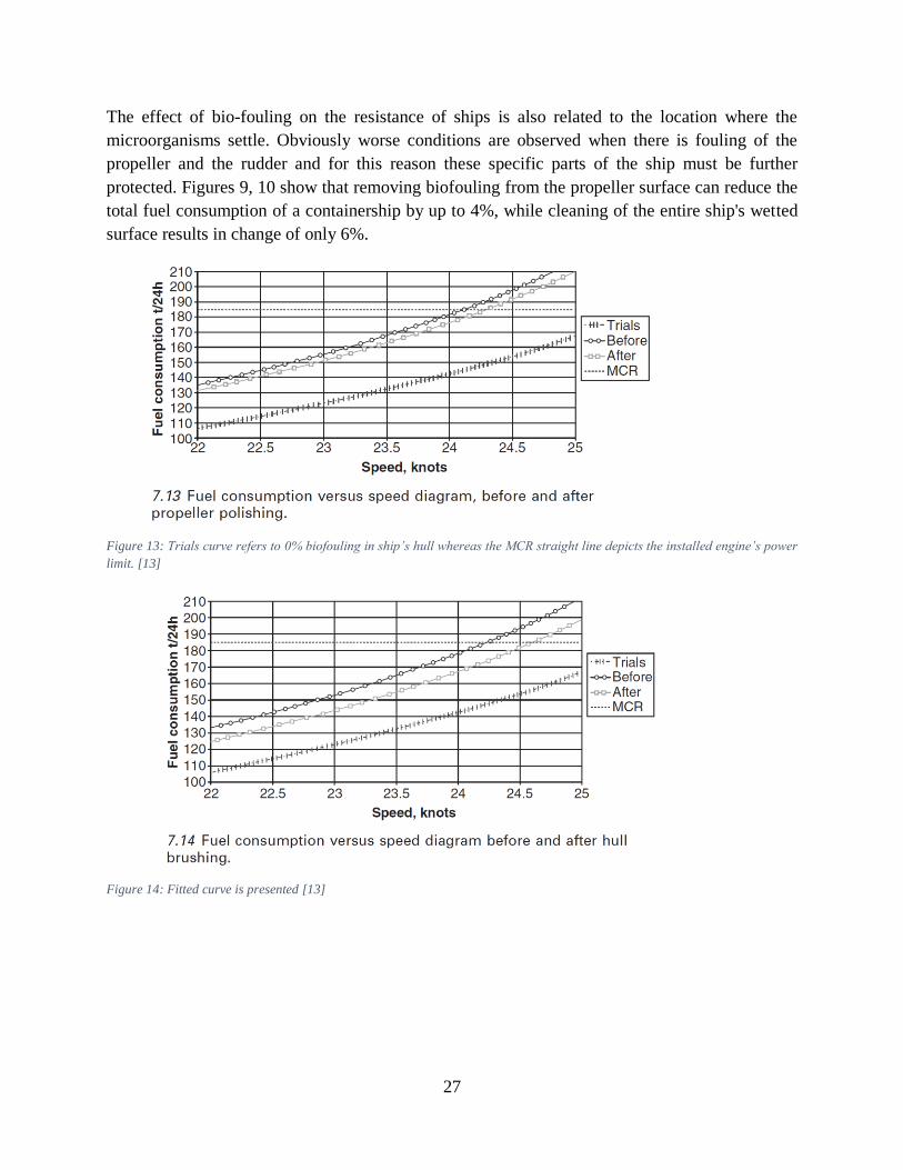
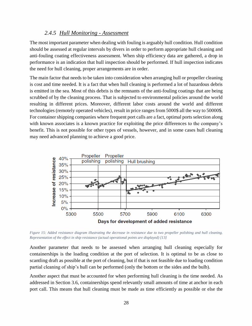
The effect of bio-fouling on the resistance of ships is also related to the location where the

microorganisms settle. Obviously worse conditions are observed when there is fouling of the

propeller and the rudder and for this reason these specific parts of the ship must be further

protected. Figures 9, 10 show that removing biofouling from the propeller surface can reduce the

total fuel consumption of a containership by up to 4%, while cleaning of the entire ship's wetted

surface results in change of only 6%.

Figure 13: Trials curve refers to 0% biofouling in ship’s hull whereas the MCR straight line depicts the installed engine’s power

limit. [13]

Figure 14: Fitted curve is presented [13]

28

2.4.5 Hull Monitoring - Assessment

The most important parameter when dealing with fouling is arguably hull condition. Hull condition

should be assessed at regular intervals by divers in order to perform appropriate hull cleaning and

anti-fouling coating effectiveness assessment. When ship efficiency data are gathered, a drop in

performance is an indication that hull inspection should be performed. If hull inspection indicates

the need for hull cleaning, proper arrangements are in order.

The main factor that needs to be taken into consideration when arranging hull or propeller cleaning

is cost and time needed. It is a fact that when hull cleaning is performed a lot of hazardous debris

is emitted in the sea. Most of this debris is the remnants of the anti-fouling coatings that are being

scrubbed of by the cleaning process. That is subjected to environmental policies around the world

resulting in different prices. Moreover, different labor costs around the world and different

technologies (remotely operated vehicles), result in price ranges from 5000$ all the way to 50000$.

For container shipping companies where frequent port calls are a fact, optimal ports selection along

with known associates is a known practice for exploiting the price differences to the company’s

benefit. This is not possible for other types of vessels, however, and in some cases hull cleaning

may need advanced planning to achieve a good price.

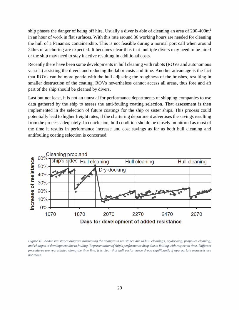
Figure 15: Added resistance diagram illustrating the decrease in resistance due to two propeller polishing and hull cleaning.

Representation of the effect in ship resistance (actual operational points are displayed) [13]

Another parameter that needs to be assessed when arranging hull cleaning especially for

containerships is the loading condition at the port of selection. It is optimal to be as close to

scantling draft as possible at the port of cleaning, but if that is not feasible due to loading condition

partial cleaning of ship’s hull can be performed (only the bottom or the sides and the bulb).

Another aspect that must be accounted for when performing hull cleaning is the time needed. As

addressed in Section 3.6, containerships spend relevantly small amounts of time at anchor in each

port call. This means that hull cleaning must be made as time efficiently as possible or else the

29

ship phases the danger of being off hire. Usually a diver is able of cleaning an area of 200-400m2

in an hour of work in flat surfaces. With this rate around 36 working hours are needed for cleaning

the hull of a Panamax containership. This is not feasible during a normal port call when around

24hrs of anchoring are expected. It becomes clear thus that multiple divers may need to be hired

or the ship may need to stay inactive resulting in additional costs.

Recently there have been some developments in hull cleaning with robots (ROVs and autonomous

vessels) assisting the divers and reducing the labor costs and time. Another advantage is the fact

that ROVs can be more gentle with the hull adjusting the roughness of the brushes, resulting in

smaller destruction of the coating. ROVs nevertheless cannot access all areas, thus fore and aft

part of the ship should be cleaned by divers.

Last but not least, it is not an unusual for performance departments of shipping companies to use

data gathered by the ship to assess the anti-fouling coating selection. That assessment is then

implemented in the selection of future coatings for the ship or sister ships. This process could

potentially lead to higher freight rates, if the chartering department advertises the savings resulting

from the process adequately. In conclusion, hull condition should be closely monitored as most of

the time it results in performance increase and cost savings as far as both hull cleaning and

antifouling coating selection is concerned.

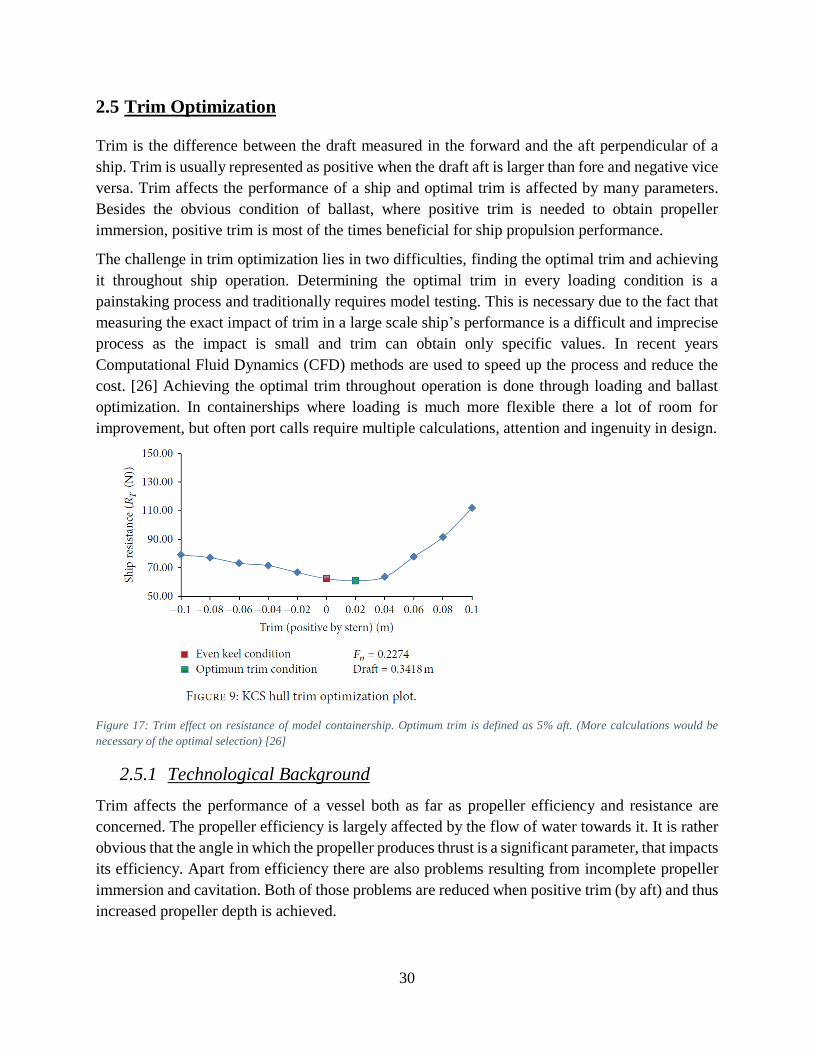
Figure 16: Added resistance diagram illustrating the changes in resistance due to hull cleanings, drydocking, propeller cleaning,

and changes in development due to fouling. Representation of ship's performance drop due to fouling with respect to time. Different

procedures are represented along the time line. It is clear that hull performance drops significantly if appropriate measures are

not taken.

30

2.5 Trim Optimization

Trim is the difference between the draft measured in the forward and the aft perpendicular of a

ship. Trim is usually represented as positive when the draft aft is larger than fore and negative vice

versa. Trim affects the performance of a ship and optimal trim is affected by many parameters.

Besides the obvious condition of ballast, where positive trim is needed to obtain propeller

immersion, positive trim is most of the times beneficial for ship propulsion performance.

The challenge in trim optimization lies in two difficulties, finding the optimal trim and achieving

it throughout ship operation. Determining the optimal trim in every loading condition is a

painstaking process and traditionally requires model testing. This is necessary due to the fact that

measuring the exact impact of trim in a large scale ship’s performance is a difficult and imprecise

process as the impact is small and trim can obtain only specific values. In recent years

Computational Fluid Dynamics (CFD) methods are used to speed up the process and reduce the

cost. [26] Achieving the optimal trim throughout operation is done through loading and ballast

optimization. In containerships where loading is much more flexible there a lot of room for

improvement, but often port calls require multiple calculations, attention and ingenuity in design.

Figure 17: Trim effect on resistance of model containership. Optimum trim is defined as 5% aft. (More calculations would be

necessary of the optimal selection) [26]

2.5.1 Technological Background

Trim affects the performance of a vessel both as far as propeller efficiency and resistance are

concerned. The propeller efficiency is largely affected by the flow of water towards it. It is rather

obvious that the angle in which the propeller produces thrust is a significant parameter, that impacts

its efficiency. Apart from efficiency there are also problems resulting from incomplete propeller

immersion and cavitation. Both of those problems are reduced when positive trim (by aft) and thus

increased propeller depth is achieved.

31

As far as resistance is concerned, trim affects both the wetted surface area of a ship and its

resistance coefficients. Wetted Surface area is generally increased when trim is increased in Full

Load, although that is not true for all loading conditions and ship types.

As far as resistance coefficients are concerned, it has been observed that positive trim results in a

reduction in wave coefficient. This reduction in higher velocities is enough to counter the increased

wetted surface area and results in reduced total resistance compared to negative trim. [31 / pg. 84]

What is more, trim is a dynamic phenomenon affected by the operational profile of a ship. As a

general principle trim remains steady or decreases slightly for reduced vessel velocities and

increases (more positive) in higher speeds. Therefore, one has to account for the operational profile

of the vessel under consideration in order to make proper optimization of its trim. [31 / pg. 84 &

pg. 159]

Another important aspect is the effect of trim under finite depth canals. This is a factor that can

result in accidents and careful attention should be given to it. When sailing in places of reduced

depth, trim is usually increased (by stern) along with the overall draft, as a byproduct of the

Bernoulli principle. Therefore, ships that are designed pass through sea routes of restricted depth

canals require additional attention. [31 / pg. 86]

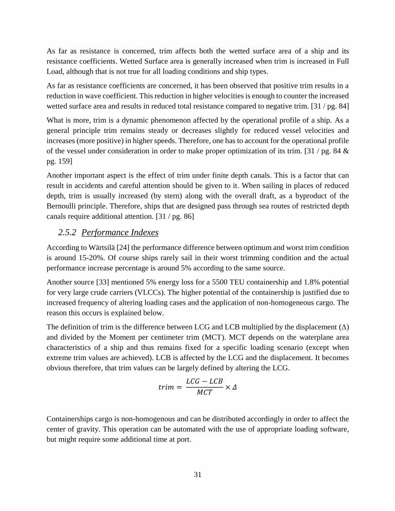
2.5.2 Performance Indexes

According to Wärtsilä [24] the performance difference between optimum and worst trim condition

is around 15-20%. Of course ships rarely sail in their worst trimming condition and the actual

performance increase percentage is around 5% according to the same source.

Another source [33] mentioned 5% energy loss for a 5500 TEU containership and 1.8% potential

for very large crude carriers (VLCCs). The higher potential of the containership is justified due to

increased frequency of altering loading cases and the application of non-homogeneous cargo. The

reason this occurs is explained below.

The definition of trim is the difference between LCG and LCB multiplied by the displacement (Δ)

and divided by the Moment per centimeter trim (MCT). MCT depends on the waterplane area

characteristics of a ship and thus remains fixed for a specific loading scenario (except when

extreme trim values are achieved). LCB is affected by the LCG and the displacement. It becomes

obvious therefore, that trim values can be largely defined by altering the LCG.

𝑡𝑟𝑖𝑚 = 𝐿𝐶𝐺 − 𝐿𝐶𝐵

𝑀𝐶𝑇× 𝛥

Containerships cargo is non-homogenous and can be distributed accordingly in order to affect the

center of gravity. This operation can be automated with the use of appropriate loading software,

but might require some additional time at port.

32

2.5.3 Feasibility

As analyzed to a greater extend in Section 3.6, trim optimization in an already operational ship is

a difficult procedure as trim can only achieve preselected values. Decreasing or increasing the size

of ballast tanks is a tedious procedure and is only performed in cases of stability regulation issues.

It is significant therefore to design a ship to be able to maintain optimum trim or arrange its cargo

in way to assist in this operation.

2.6 Ballast Water Reduction

Recently ballast water came under the attention of the IMO as invasive species were under

suspicion of being transferred in ships’ ballast tanks. This resulted in big problems to marine

ecosystems that have been affected in more than one ways from International shipping (Suez, TBT

coatings, etc.). The result was the introduction of Ballast Water Treatment Systems (BWTS) as a

means to comply with 2018 IMO Ballast Water Management System (BWMS) introduction.

Ballast water is the means to achieving propeller immersion in empty loading condition and

optimal trim in any loading condition other than Full Load Departure (FLD) as it has already been

mentioned. Also, ballast water acts favorably to the ships’ stability. Especially when it comes to

containerships where partial loading is the most frequent loading scenario, ballast water

distribution can play an important role in maintaining optimum trim, propeller immersion and

stability.

It is a fact nevertheless that containerships rarely travel without any cargo and thus ballast

minimization can be achieved as a result of the cargo carried and the reduced need for stability and

propeller immersion. What is more, containerships are able to load on a non-uniform way and thus

trim optimization is much more easily achievable.

2.6.1 Technological Background

Empty ship’s weight (the weight of the steel structure or Lightship – LS) amounts to 10-20% of

the overall full load displacement of large merchant ships. This ratio can be further increased up

to 30% for containerships. It is a fact that with this weight alone merchant ships cannot obtain the

required draft to maintain propeller immersion and proper stability. That is the reason why Ballast

Water Tanks exist in every ship and during cargo unloading they are filled with seawater to

increase the weight carried by the ship resulting in propeller immersion and stability. Ballast tanks

can also assist in maintaining the optimum trim as already indicated by Section 3.5.

Ballast tanks are located in the bottom of the ship throughout the cargo area (for stability reasons)

and typically two tanks are located in the bow and stern (serving trim optimization purposes). In

some types of ships, such as tankers, ballast water tanks are obligatory, since these ships are

required to have a double hull not filled with cargo. In other types such as bulk carriers the shape

of ballast tanks assists in cargo loading (topside tanks) and discharge (hopper). Containership

33

water ballast tanks are usually in a shape that provides maximum usable space for loading

containers (cubes).

To reduce ballast water tanks volume there are a number of considerations in order. As already

expressed the greatest concerns are stability and propeller immersion.

As far as stability is concerned propositions include the increase in beam. [33] Of course merchant

ships dimensions are not always available for modification, as many of them are associated with

limitations imposed by port facilities or shipping passages (Suez Canal, Panama Canal, Straits of

Malacca, etc.). What is more, an increase in a ships beam might have an adverse effect in the ship’s

hydrodynamic shape, increasing its wetted surface without increasing its capacity.

Reduced ballast results in reduced ballast condition draft. This can result in reduced propeller

immersion or increased trim values. Propeller immersion is essential for maintaining proper

propeller condition. When a propeller reaches above the waterline it creates eccentric thrust that

could lead to damages on the shaft due to bending moments and vibrations. What is more, due to

waves part of the shaft can be found above the water. In such a case, significant problems will

arise in the shaft lubrication system. If high trim values are needed to achieve proper propeller

immersion the fore part of the ship will be experiencing heavy slamming causing structural

problems.

One way to cope with this problem is by reducing the propeller size. This can be done by using

more volumetric efficient propellers, such as highly bladed ones. It should be noted that

containerships are traditionally designed with 5-bladed and in some cases 6-bladed propellers for

achieving increased speeds and this method may not be feasible for some ships. This is another

reason for careful consideration along with the fact that heavy bladed propellers are more

expensive and slightly less efficient.

All things considered, 40% reduction of ballast water is considered to be achievable, resulting in

increased cargo space. What is more, analysis has shown that average container weight more than

makes up for stability purposes and stability problems are not going to be an issue, from this

reduction. [27 / pg.64]

34

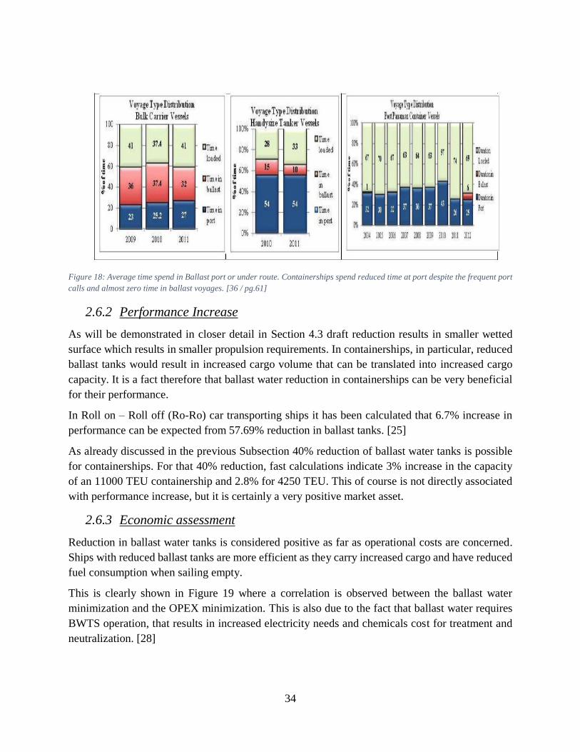
Figure 18: Average time spend in Ballast port or under route. Containerships spend reduced time at port despite the frequent port

calls and almost zero time in ballast voyages. [36 / pg.61]

2.6.2 Performance Increase

As will be demonstrated in closer detail in Section 4.3 draft reduction results in smaller wetted

surface which results in smaller propulsion requirements. In containerships, in particular, reduced

ballast tanks would result in increased cargo volume that can be translated into increased cargo

capacity. It is a fact therefore that ballast water reduction in containerships can be very beneficial

for their performance.

In Roll on – Roll off (Ro-Ro) car transporting ships it has been calculated that 6.7% increase in

performance can be expected from 57.69% reduction in ballast tanks. [25]

As already discussed in the previous Subsection 40% reduction of ballast water tanks is possible

for containerships. For that 40% reduction, fast calculations indicate 3% increase in the capacity

of an 11000 TEU containership and 2.8% for 4250 TEU. This of course is not directly associated

with performance increase, but it is certainly a very positive market asset.

2.6.3 Economic assessment

Reduction in ballast water tanks is considered positive as far as operational costs are concerned.

Ships with reduced ballast tanks are more efficient as they carry increased cargo and have reduced

fuel consumption when sailing empty.

This is clearly shown in Figure 19 where a correlation is observed between the ballast water

minimization and the OPEX minimization. This is also due to the fact that ballast water requires

BWTS operation, that results in increased electricity needs and chemicals cost for treatment and

neutralization. [28]

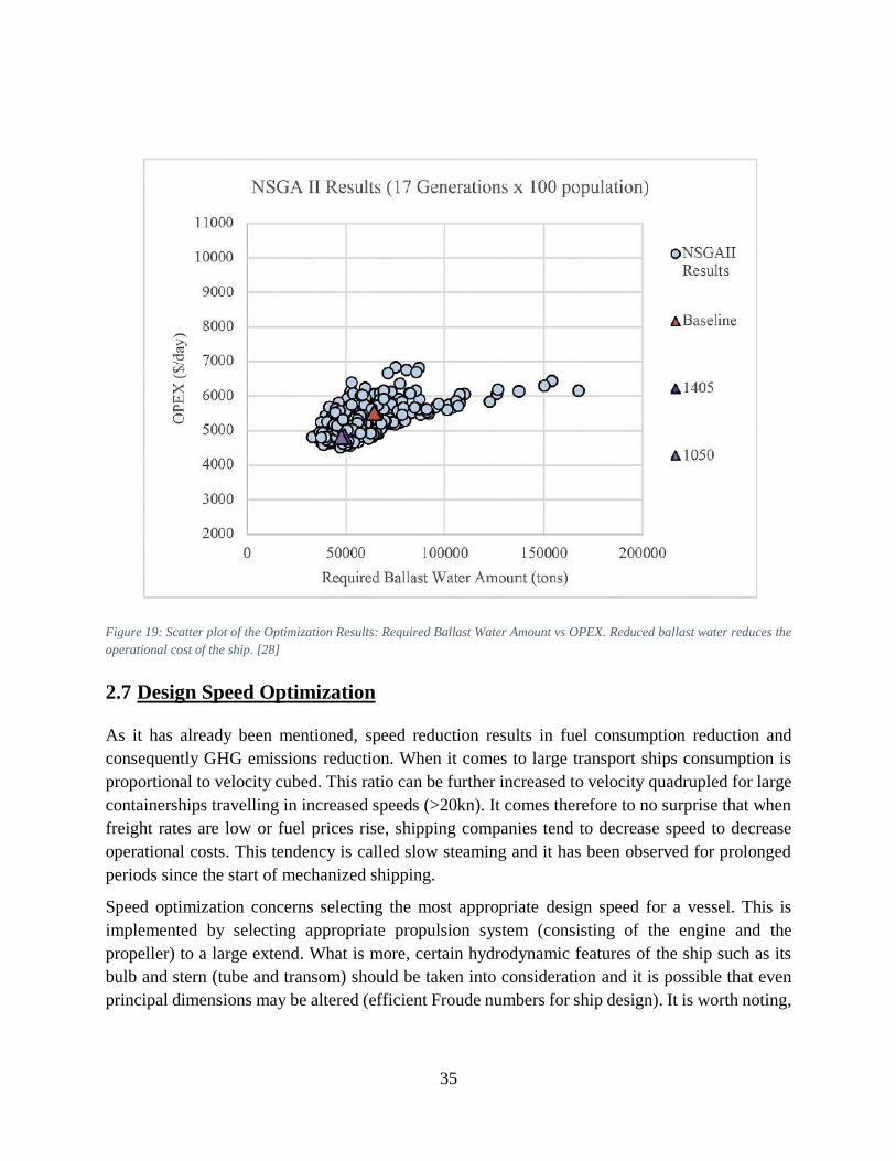
35

Figure 19: Scatter plot of the Optimization Results: Required Ballast Water Amount vs OPEX. Reduced ballast water reduces the

operational cost of the ship. [28]

2.7 Design Speed Optimization

As it has already been mentioned, speed reduction results in fuel consumption reduction and

consequently GHG emissions reduction. When it comes to large transport ships consumption is

proportional to velocity cubed. This ratio can be further increased to velocity quadrupled for large

containerships travelling in increased speeds (>20kn). It comes therefore to no surprise that when

freight rates are low or fuel prices rise, shipping companies tend to decrease speed to decrease

operational costs. This tendency is called slow steaming and it has been observed for prolonged

periods since the start of mechanized shipping.

Speed optimization concerns selecting the most appropriate design speed for a vessel. This is

implemented by selecting appropriate propulsion system (consisting of the engine and the

propeller) to a large extend. What is more, certain hydrodynamic features of the ship such as its

bulb and stern (tube and transom) should be taken into consideration and it is possible that even

principal dimensions may be altered (efficient Froude numbers for ship design). It is worth noting,

36

that ship optimization can occur even after the ship has been launched with options such as derating

and bulb retrofit, but there is an additional cost to it.

2.7.1 Technical Considerations

There are many options to consider when selecting appropriate design speed for a vessel. The main

criteria stem from the operational or market analysis that demonstrate the transport need the ship

will need to cover, but there are also technical limitations. In recent years there is a tendency for

ships to select lower design speed in order to align with IMO and other stakeholders’ policies for

transporting efficiency. The reason for this will be analyzed below.

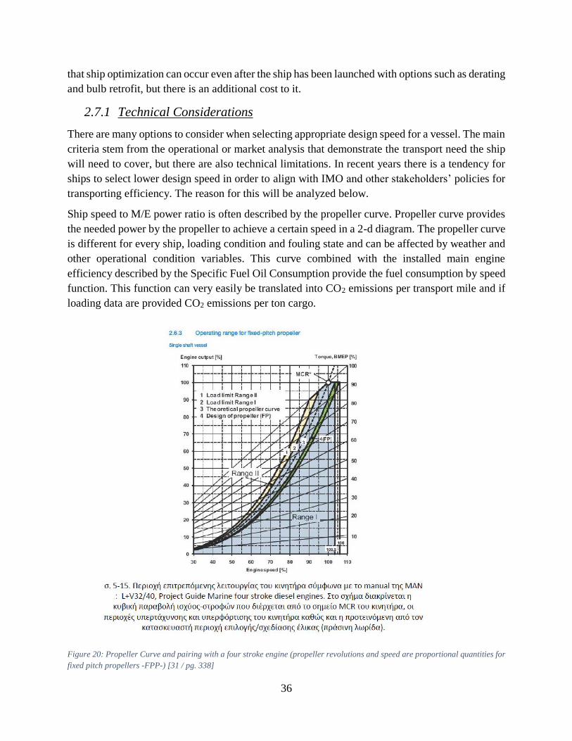
Ship speed to M/E power ratio is often described by the propeller curve. Propeller curve provides

the needed power by the propeller to achieve a certain speed in a 2-d diagram. The propeller curve

is different for every ship, loading condition and fouling state and can be affected by weather and

other operational condition variables. This curve combined with the installed main engine

efficiency described by the Specific Fuel Oil Consumption provide the fuel consumption by speed

function. This function can very easily be translated into CO2 emissions per transport mile and if

loading data are provided CO2 emissions per ton cargo.

Figure 20: Propeller Curve and pairing with a four stroke engine (propeller revolutions and speed are proportional quantities for

fixed pitch propellers -FPP-) [31 / pg. 338]

37

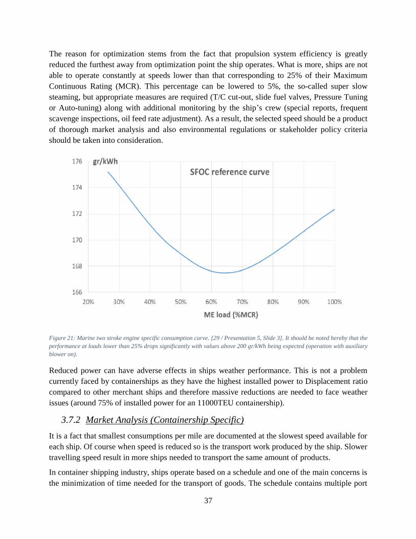
The reason for optimization stems from the fact that propulsion system efficiency is greatly

reduced the furthest away from optimization point the ship operates. What is more, ships are not

able to operate constantly at speeds lower than that corresponding to 25% of their Maximum

Continuous Rating (MCR). This percentage can be lowered to 5%, the so-called super slow

steaming, but appropriate measures are required (T/C cut-out, slide fuel valves, Pressure Tuning

or Auto-tuning) along with additional monitoring by the ship’s crew (special reports, frequent

scavenge inspections, oil feed rate adjustment). As a result, the selected speed should be a product

of thorough market analysis and also environmental regulations or stakeholder policy criteria

should be taken into consideration.

Figure 21: Marine two stroke engine specific consumption curve. [29 / Presentation 5, Slide 3]. It should be noted hereby that the

performance at loads lower than 25% drops significantly with values above 200 gr/kWh being expected (operation with auxiliary

blower on).

Reduced power can have adverse effects in ships weather performance. This is not a problem

currently faced by containerships as they have the highest installed power to Displacement ratio

compared to other merchant ships and therefore massive reductions are needed to face weather

issues (around 75% of installed power for an 11000TEU containership).

3.7.2 Market Analysis (Containership Specific)

It is a fact that smallest consumptions per mile are documented at the slowest speed available for

each ship. Of course when speed is reduced so is the transport work produced by the ship. Slower

travelling speed result in more ships needed to transport the same amount of products.

In container shipping industry, ships operate based on a schedule and one of the main concerns is

the minimization of time needed for the transport of goods. The schedule contains multiple port

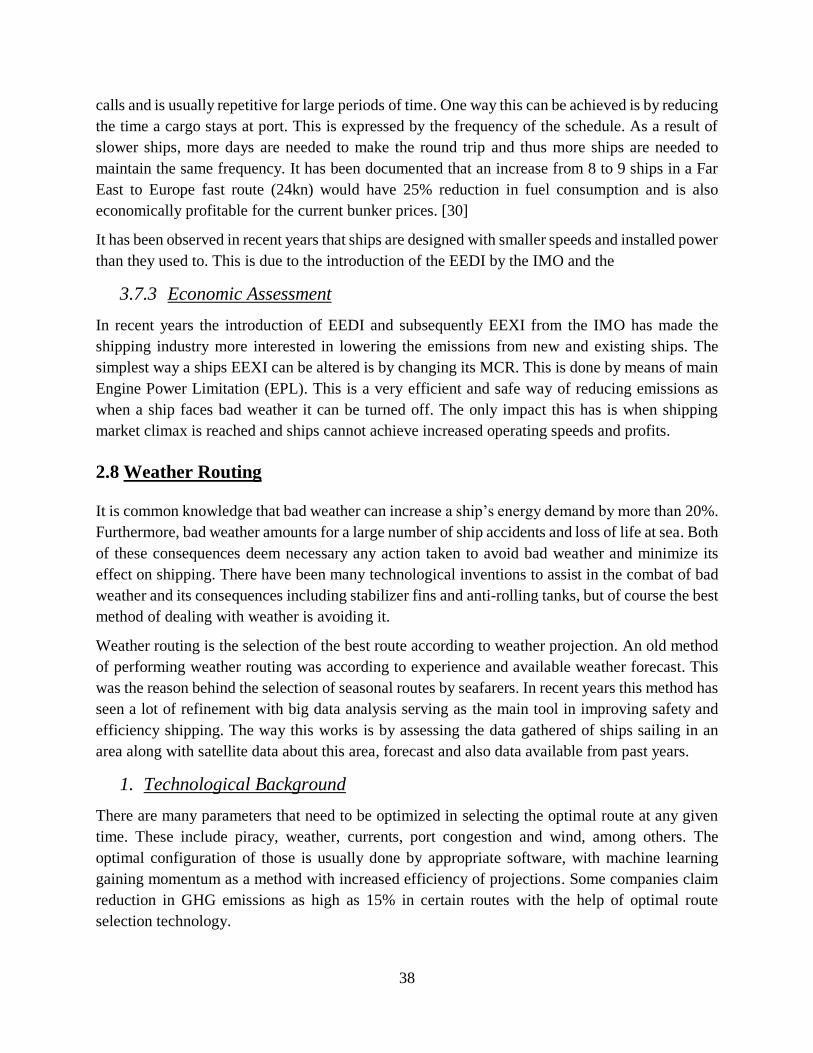
38

calls and is usually repetitive for large periods of time. One way this can be achieved is by reducing

the time a cargo stays at port. This is expressed by the frequency of the schedule. As a result of

slower ships, more days are needed to make the round trip and thus more ships are needed to

maintain the same frequency. It has been documented that an increase from 8 to 9 ships in a Far

East to Europe fast route (24kn) would have 25% reduction in fuel consumption and is also

economically profitable for the current bunker prices. [30]

It has been observed in recent years that ships are designed with smaller speeds and installed power

than they used to. This is due to the introduction of the EEDI by the IMO and the

3.7.3 Economic Assessment

In recent years the introduction of EEDI and subsequently EEXI from the IMO has made the

shipping industry more interested in lowering the emissions from new and existing ships. The

simplest way a ships EEXI can be altered is by changing its MCR. This is done by means of main

Engine Power Limitation (EPL). This is a very efficient and safe way of reducing emissions as

when a ship faces bad weather it can be turned off. The only impact this has is when shipping

market climax is reached and ships cannot achieve increased operating speeds and profits.

2.8 Weather Routing

It is common knowledge that bad weather can increase a ship’s energy demand by more than 20%.

Furthermore, bad weather amounts for a large number of ship accidents and loss of life at sea. Both

of these consequences deem necessary any action taken to avoid bad weather and minimize its

effect on shipping. There have been many technological inventions to assist in the combat of bad

weather and its consequences including stabilizer fins and anti-rolling tanks, but of course the best

method of dealing with weather is avoiding it.

Weather routing is the selection of the best route according to weather projection. An old method

of performing weather routing was according to experience and available weather forecast. This

was the reason behind the selection of seasonal routes by seafarers. In recent years this method has

seen a lot of refinement with big data analysis serving as the main tool in improving safety and

efficiency shipping. The way this works is by assessing the data gathered of ships sailing in an

area along with satellite data about this area, forecast and also data available from past years.

1. Technological Background

There are many parameters that need to be optimized in selecting the optimal route at any given

time. These include piracy, weather, currents, port congestion and wind, among others. The

optimal configuration of those is usually done by appropriate software, with machine learning

gaining momentum as a method with increased efficiency of projections. Some companies claim

reduction in GHG emissions as high as 15% in certain routes with the help of optimal route

selection technology.

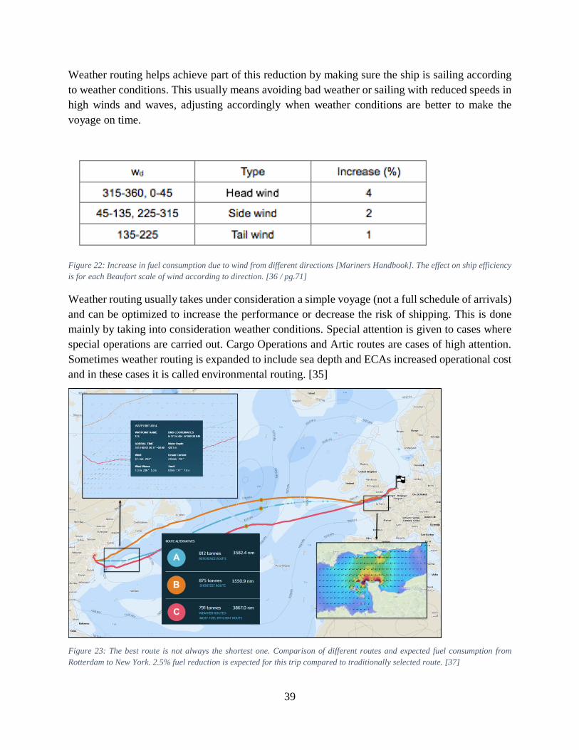
39

Weather routing helps achieve part of this reduction by making sure the ship is sailing according

to weather conditions. This usually means avoiding bad weather or sailing with reduced speeds in

high winds and waves, adjusting accordingly when weather conditions are better to make the

voyage on time.

Figure 22: Increase in fuel consumption due to wind from different directions [Mariners Handbook]. The effect on ship efficiency

is for each Beaufort scale of wind according to direction. [36 / pg.71]

Weather routing usually takes under consideration a simple voyage (not a full schedule of arrivals)

and can be optimized to increase the performance or decrease the risk of shipping. This is done

mainly by taking into consideration weather conditions. Special attention is given to cases where

special operations are carried out. Cargo Operations and Artic routes are cases of high attention.

Sometimes weather routing is expanded to include sea depth and ECAs increased operational cost

and in these cases it is called environmental routing. [35]

Figure 23: The best route is not always the shortest one. Comparison of different routes and expected fuel consumption from

Rotterdam to New York. 2.5% fuel reduction is expected for this trip compared to traditionally selected route. [37]

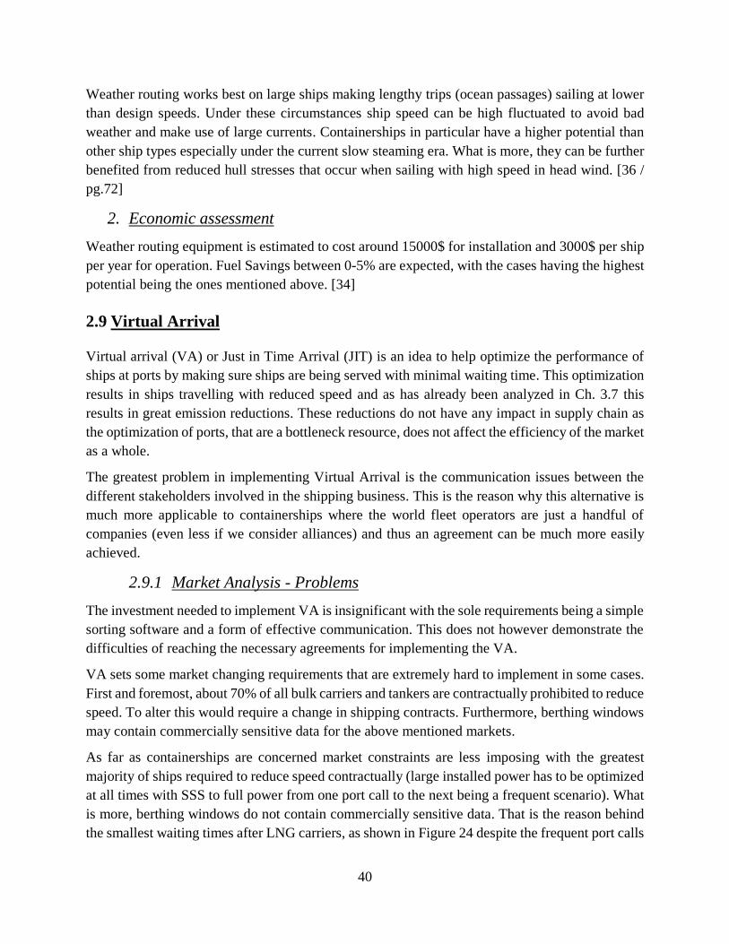
40

Weather routing works best on large ships making lengthy trips (ocean passages) sailing at lower

than design speeds. Under these circumstances ship speed can be high fluctuated to avoid bad

weather and make use of large currents. Containerships in particular have a higher potential than

other ship types especially under the current slow steaming era. What is more, they can be further

benefited from reduced hull stresses that occur when sailing with high speed in head wind. [36 /

pg.72]

2. Economic assessment

Weather routing equipment is estimated to cost around 15000$ for installation and 3000$ per ship

per year for operation. Fuel Savings between 0-5% are expected, with the cases having the highest

potential being the ones mentioned above. [34]

2.9 Virtual Arrival

Virtual arrival (VA) or Just in Time Arrival (JIT) is an idea to help optimize the performance of

ships at ports by making sure ships are being served with minimal waiting time. This optimization

results in ships travelling with reduced speed and as has already been analyzed in Ch. 3.7 this

results in great emission reductions. These reductions do not have any impact in supply chain as

the optimization of ports, that are a bottleneck resource, does not affect the efficiency of the market

as a whole.

The greatest problem in implementing Virtual Arrival is the communication issues between the

different stakeholders involved in the shipping business. This is the reason why this alternative is

much more applicable to containerships where the world fleet operators are just a handful of

companies (even less if we consider alliances) and thus an agreement can be much more easily

achieved.

2.9.1 Market Analysis - Problems

The investment needed to implement VA is insignificant with the sole requirements being a simple

sorting software and a form of effective communication. This does not however demonstrate the

difficulties of reaching the necessary agreements for implementing the VA.

VA sets some market changing requirements that are extremely hard to implement in some cases.

First and foremost, about 70% of all bulk carriers and tankers are contractually prohibited to reduce

speed. To alter this would require a change in shipping contracts. Furthermore, berthing windows

may contain commercially sensitive data for the above mentioned markets.

As far as containerships are concerned market constraints are less imposing with the greatest

majority of ships required to reduce speed contractually (large installed power has to be optimized

at all times with SSS to full power from one port call to the next being a frequent scenario). What

is more, berthing windows do not contain commercially sensitive data. That is the reason behind

the smallest waiting times after LNG carriers, as shown in Figure 24 despite the frequent port calls

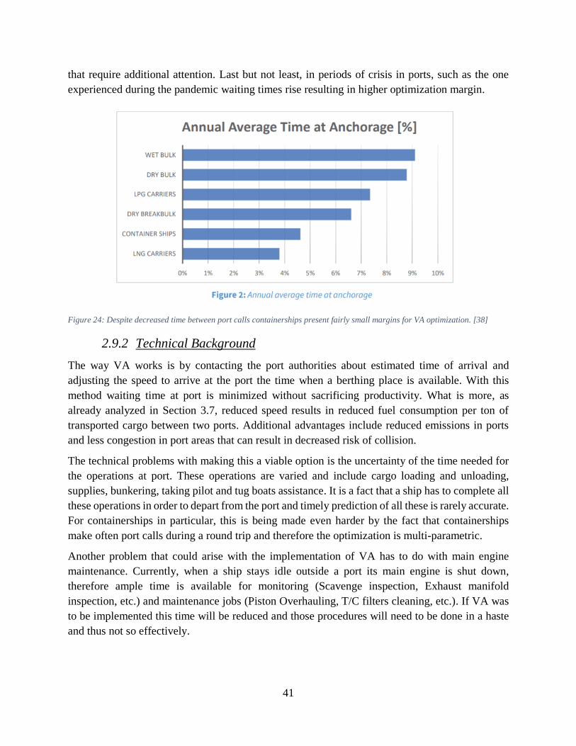
41

that require additional attention. Last but not least, in periods of crisis in ports, such as the one

experienced during the pandemic waiting times rise resulting in higher optimization margin.

Figure 24: Despite decreased time between port calls containerships present fairly small margins for VA optimization. [38]

2.9.2 Technical Background

The way VA works is by contacting the port authorities about estimated time of arrival and

adjusting the speed to arrive at the port the time when a berthing place is available. With this

method waiting time at port is minimized without sacrificing productivity. What is more, as

already analyzed in Section 3.7, reduced speed results in reduced fuel consumption per ton of

transported cargo between two ports. Additional advantages include reduced emissions in ports

and less congestion in port areas that can result in decreased risk of collision.

The technical problems with making this a viable option is the uncertainty of the time needed for

the operations at port. These operations are varied and include cargo loading and unloading,

supplies, bunkering, taking pilot and tug boats assistance. It is a fact that a ship has to complete all

these operations in order to depart from the port and timely prediction of all these is rarely accurate.

For containerships in particular, this is being made even harder by the fact that containerships

make often port calls during a round trip and therefore the optimization is multi-parametric.

Another problem that could arise with the implementation of VA has to do with main engine

maintenance. Currently, when a ship stays idle outside a port its main engine is shut down,

therefore ample time is available for monitoring (Scavenge inspection, Exhaust manifold

inspection, etc.) and maintenance jobs (Piston Overhauling, T/C filters cleaning, etc.). If VA was

to be implemented this time will be reduced and those procedures will need to be done in a haste

and thus not so effectively.

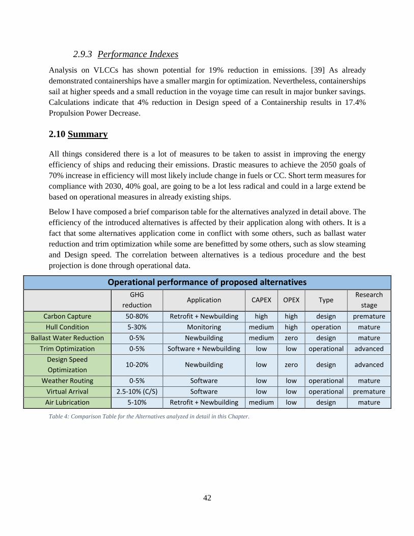
42

2.9.3 Performance Indexes

Analysis on VLCCs has shown potential for 19% reduction in emissions. [39] As already

demonstrated containerships have a smaller margin for optimization. Nevertheless, containerships

sail at higher speeds and a small reduction in the voyage time can result in major bunker savings.

Calculations indicate that 4% reduction in Design speed of a Containership results in 17.4%

Propulsion Power Decrease.

2.10 Summary

All things considered there is a lot of measures to be taken to assist in improving the energy

efficiency of ships and reducing their emissions. Drastic measures to achieve the 2050 goals of

70% increase in efficiency will most likely include change in fuels or CC. Short term measures for

compliance with 2030, 40% goal, are going to be a lot less radical and could in a large extend be

based on operational measures in already existing ships.

Below I have composed a brief comparison table for the alternatives analyzed in detail above. The

efficiency of the introduced alternatives is affected by their application along with others. It is a

fact that some alternatives application come in conflict with some others, such as ballast water

reduction and trim optimization while some are benefitted by some others, such as slow steaming

and Design speed. The correlation between alternatives is a tedious procedure and the best

projection is done through operational data.

Operational performance of proposed alternatives

GHG

reduction Application CAPEX OPEX Type

Research

stage

Carbon Capture 50-80% Retrofit + Newbuilding high high design premature

Hull Condition 5-30% Monitoring medium high operation mature

Ballast Water Reduction 0-5% Newbuilding medium zero design mature

Trim Optimization 0-5% Software + Newbuilding low low operational advanced

Design Speed

Optimization 10-20% Newbuilding low zero design advanced

Weather Routing 0-5% Software low low operational mature

Virtual Arrival 2.5-10% (C/S) Software low low operational premature

Air Lubrication 5-10% Retrofit + Newbuilding medium low design mature

Table 4: Comparison Table for the Alternatives analyzed in detail in this Chapter.

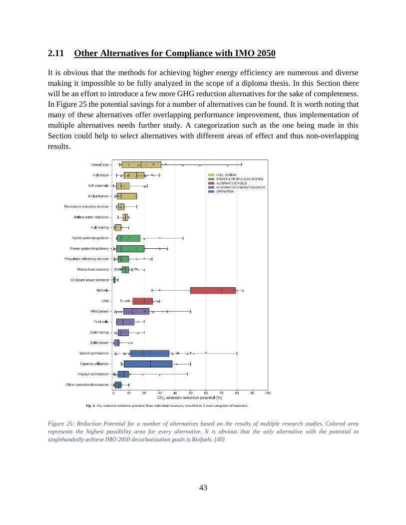
43

2.11 Other Alternatives for Compliance with IΜΟ 2050

It is obvious that the methods for achieving higher energy efficiency are numerous and diverse

making it impossible to be fully analyzed in the scope of a diploma thesis. In this Section there

will be an effort to introduce a few more GHG reduction alternatives for the sake of completeness.

In Figure 25 the potential savings for a number of alternatives can be found. It is worth noting that

many of these alternatives offer overlapping performance improvement, thus implementation of

multiple alternatives needs further study. A categorization such as the one being made in this

Section could help to select alternatives with different areas of effect and thus non-overlapping

results.

Figure 25: Reduction Potential for a number of alternatives based on the results of multiple research studies. Colored area

represents the highest possibility area for every alternative. It is obvious that the only alternative with the potential to

singlehandedly achieve IMO 2050 decarbonization goals is Biofuels. [40]

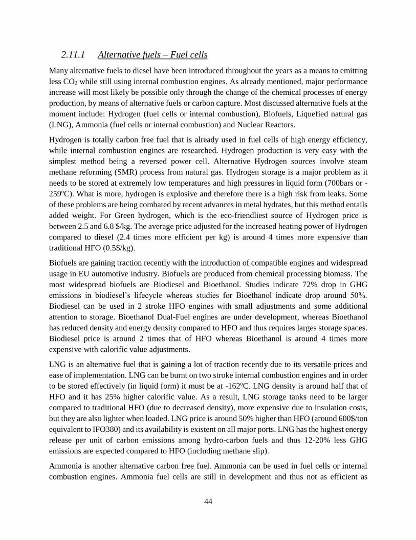
44

2.11.1 Alternative fuels – Fuel cells

Many alternative fuels to diesel have been introduced throughout the years as a means to emitting

less CO2 while still using internal combustion engines. As already mentioned, major performance

increase will most likely be possible only through the change of the chemical processes of energy

production, by means of alternative fuels or carbon capture. Most discussed alternative fuels at the

moment include: Hydrogen (fuel cells or internal combustion), Biofuels, Liquefied natural gas

(LNG), Ammonia (fuel cells or internal combustion) and Nuclear Reactors.

Hydrogen is totally carbon free fuel that is already used in fuel cells of high energy efficiency,

while internal combustion engines are researched. Hydrogen production is very easy with the

simplest method being a reversed power cell. Alternative Hydrogen sources involve steam

methane reforming (SMR) process from natural gas. Hydrogen storage is a major problem as it

needs to be stored at extremely low temperatures and high pressures in liquid form (700bars or -

259oC). What is more, hydrogen is explosive and therefore there is a high risk from leaks. Some

of these problems are being combated by recent advances in metal hydrates, but this method entails

added weight. For Green hydrogen, which is the eco-friendliest source of Hydrogen price is

between 2.5 and 6.8 $/kg. The average price adjusted for the increased heating power of Hydrogen

compared to diesel (2.4 times more efficient per kg) is around 4 times more expensive than

traditional HFO (0.5$/kg).

Biofuels are gaining traction recently with the introduction of compatible engines and widespread

usage in EU automotive industry. Biofuels are produced from chemical processing biomass. The

most widespread biofuels are Biodiesel and Bioethanol. Studies indicate 72% drop in GHG

emissions in biodiesel’s lifecycle whereas studies for Bioethanol indicate drop around 50%.

Biodiesel can be used in 2 stroke HFO engines with small adjustments and some additional

attention to storage. Bioethanol Dual-Fuel engines are under development, whereas Bioethanol

has reduced density and energy density compared to HFO and thus requires larges storage spaces.

Biodiesel price is around 2 times that of HFO whereas Bioethanol is around 4 times more

expensive with calorific value adjustments.

LNG is an alternative fuel that is gaining a lot of traction recently due to its versatile prices and

ease of implementation. LNG can be burnt on two stroke internal combustion engines and in order

to be stored effectively (in liquid form) it must be at -162oC. LNG density is around half that of

HFO and it has 25% higher calorific value. As a result, LNG storage tanks need to be larger

compared to traditional HFO (due to decreased density), more expensive due to insulation costs,

but they are also lighter when loaded. LNG price is around 50% higher than HFO (around 600$/ton

equivalent to IFO380) and its availability is existent on all major ports. LNG has the highest energy

release per unit of carbon emissions among hydro-carbon fuels and thus 12-20% less GHG

emissions are expected compared to HFO (including methane slip).

Ammonia is another alternative carbon free fuel. Ammonia can be used in fuel cells or internal

combustion engines. Ammonia fuel cells are still in development and thus not as efficient as

45

Hydrogen. Internal combustion engines, on the other hand, need to be mixed with Diesel or other

fuels for better combustibility, thus some GHG emissions are expected. Ammonia transportation

is less complicated than Hydrogen and LNG. Ammonia liquefaction temperature is -33oC and the

it has good volumetric efficiency (half that of LNG but still higher than Hydrogen). Its price is

around 3 times that of HFO.

Nuclear power is another alternative to power GHG emission free ships. Nuclear energy has

already been tested on board warships, but the reduced crew members of commercial ships and

the dangers associated with an accident, make the public opinion hard to shift in its favor.

Last but not least, it is worth noting that major performance increase is considered to be possible

only through the change of the chemical processes of energy production by means of alternative

fuels or carbon capture.

2.11.2 Alternative Power Sources

Wind and Sun are endless resources at sea. There are many devices fit to take advantage of these

resources and transform some of their potential to kinetic or electrical energy thus decreasing

propulsion or electrical needs of a ship.

Sails is one way this can be achieved. These are modern designs of the traditional method of

propulsion that allow for increased sails area and minimum effort by the crew.

Another alternative is flettner rotors. These rotors take advantage of the bernoulli’s fluid dynamic

principle to produce propulsive force from rotating when operating under side winds. The

installation of such devices is simple but their GHG reduction potential small. What is more, in

containerships where deck space is limited these devices will struggle to provide for any assistance.

Solar cells on the deck of a ship is a means of covering a part of its electrical energy needs. This

fraction can be a reduction in Diesel Generators (D/G) workload and thus a reduction in the ship’s

emissions. This method can be particularly useful for containerships where feeder containers

require significant energy when travelling.

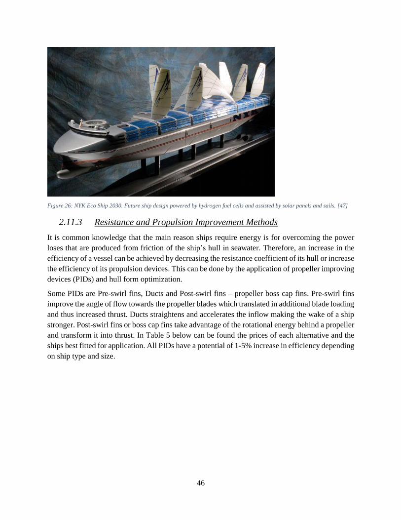
46

Figure 26: NYK Eco Ship 2030. Future ship design powered by hydrogen fuel cells and assisted by solar panels and sails. [47]

2.11.3 Resistance and Propulsion Improvement Methods

It is common knowledge that the main reason ships require energy is for overcoming the power

loses that are produced from friction of the ship’s hull in seawater. Therefore, an increase in the

efficiency of a vessel can be achieved by decreasing the resistance coefficient of its hull or increase

the efficiency of its propulsion devices. This can be done by the application of propeller improving

devices (PIDs) and hull form optimization.

Some PIDs are Pre-swirl fins, Ducts and Post-swirl fins – propeller boss cap fins. Pre-swirl fins

improve the angle of flow towards the propeller blades which translated in additional blade loading

and thus increased thrust. Ducts straightens and accelerates the inflow making the wake of a ship

stronger. Post-swirl fins or boss cap fins take advantage of the rotational energy behind a propeller

and transform it into thrust. In Table 5 below can be found the prices of each alternative and the

ships best fitted for application. All PIDs have a potential of 1-5% increase in efficiency depending

on ship type and size.

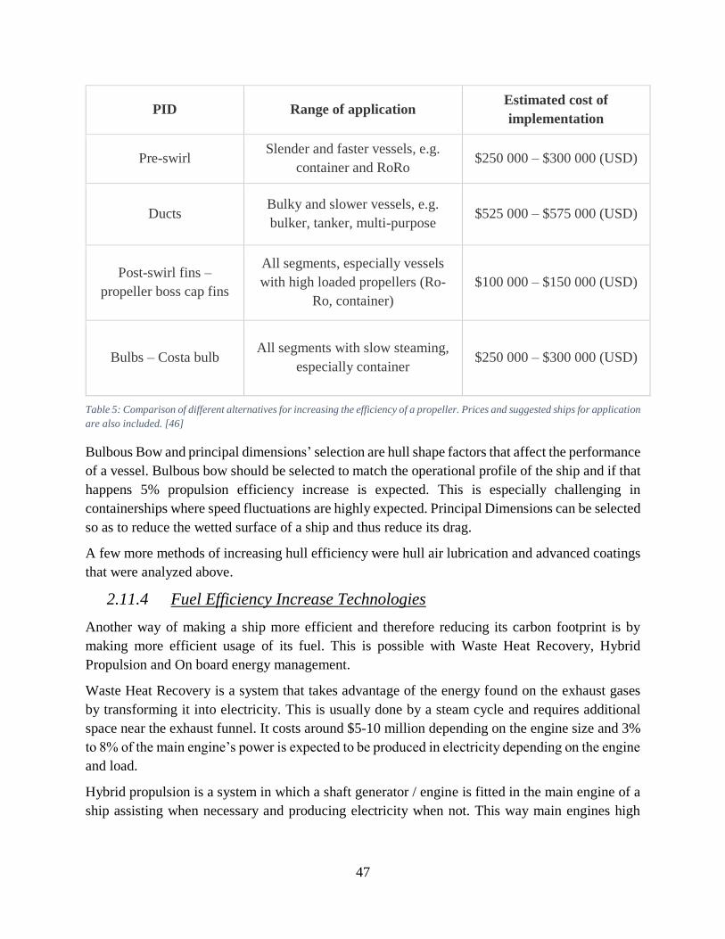
47

PID Range of application Estimated cost of

implementation

Pre-swirl Slender and faster vessels, e.g.

container and RoRo $250 000 – $300 000 (USD)

Ducts Bulky and slower vessels, e.g.

bulker, tanker, multi-purpose $525 000 – $575 000 (USD)

Post-swirl fins –

propeller boss cap fins

All segments, especially vessels

with high loaded propellers (Ro-

Ro, container)

$100 000 – $150 000 (USD)

Bulbs – Costa bulb All segments with slow steaming,

especially container $250 000 – $300 000 (USD)

Table 5: Comparison of different alternatives for increasing the efficiency of a propeller. Prices and suggested ships for application

are also included. [46]

Bulbous Bow and principal dimensions’ selection are hull shape factors that affect the performance

of a vessel. Bulbous bow should be selected to match the operational profile of the ship and if that

happens 5% propulsion efficiency increase is expected. This is especially challenging in

containerships where speed fluctuations are highly expected. Principal Dimensions can be selected

so as to reduce the wetted surface of a ship and thus reduce its drag.

A few more methods of increasing hull efficiency were hull air lubrication and advanced coatings

that were analyzed above.

2.11.4 Fuel Efficiency Increase Technologies

Another way of making a ship more efficient and therefore reducing its carbon footprint is by

making more efficient usage of its fuel. This is possible with Waste Heat Recovery, Hybrid

Propulsion and On board energy management.

Waste Heat Recovery is a system that takes advantage of the energy found on the exhaust gases

by transforming it into electricity. This is usually done by a steam cycle and requires additional

space near the exhaust funnel. It costs around $5-10 million depending on the engine size and 3%

to 8% of the main engine’s power is expected to be produced in electricity depending on the engine

and load.

Hybrid propulsion is a system in which a shaft generator / engine is fitted in the main engine of a

ship assisting when necessary and producing electricity when not. This way main engines high

48

efficiency is exploited in electricity production and GHG emissions are reduced. This is an option

not available for large commercial ships and slow speed two stroke engines.

On board energy management ensures that all electricity consuming devices operate on their best

efficiency. This measure has 1%-3% reduction potential.

49

3. Case Studies – Calculations

3.1 Introduction

As already mentioned, there is a lot of debate around which GHG reduction alternatives should be

applied, in order to better assist in the transition of the shipping business to GHG neutrality. The

problem lies in making sure the selected alternatives are cost efficient and result in the necessary

reduction in GHG emissions, for every individual ship under consideration.

In this Chapter three GHG reduction alternatives will be analyzed, that are of high relevance to the

container shipping industry. All of these ideas are already being implemented to a certain extend,

with the first one receiving little attention and the others being much more adopted.

The main focus of this Chapter will be the calculation of reduction each alternative has to offer on

containership’s emissions and the representation with appropriate indexes, along with economic

or operational evaluation. To make this calculation, the most accurate data from actual ships will

be extracted analyzed and best projected, using appropriate tools.

50

3.2 Containers Constructed from Composite Materials

Containers constructed from composite materials (or composite containers) are an alternative for

increasing the performance of containerships. This involves the application of advanced materials,

with lighter weight, in the structural parts (tare weight) of containers. This way a reduction in the

overall weight of the ship is made, without affecting its Payload. Although advanced materials in

shipping are not radical, with high tensile steel and aluminum superstructures being common case

nowadays, composite materials have yet to find usage in the shipping industry.

This method has been largely ignored, due to the high cost of the composite materials that deem it

economically inefficient. That could nevertheless change, as the requirements for highly efficient

ships the IMO has set for 2050, might increase the acceptance by shipping firms of initiatives, that

can reduce their carbon footprint. These regulations, along with the increased versatility of

composite containers, both as far as longevity and foldability are concerned, could make them a

very interesting option in the future.

In this Section, the effect of the weight reduction on the ship’s efficiency will be the main focus.

This effect will be analyzed using appropriate indexes, in order to better demonstrate the impact it

has on the ship’s performance and emissions. An important step to evaluate this change will be the

prediction of the new fuel consumption, according to the change in the total Displacement. This

evaluation will be analyzed in-depth to achieve maximum precision.

3.2.1 Calculations Scope / method

To better predict the effect weight reduction has on emissions, Resistance force and subsequently,

Propulsion power reduction was needed. Once Propulsion power requirements are calculated, it

becomes straightforward to find the true emissions reduction potential. Extracted results can then

be analyzed using appropriate Indexes, similar to EEDI.

In order to predict resistance reduction, the Holtrop-Mennen method was used. To accelerate

calculations HydroComp NavCad 2013 Evaluation Demo Software was used (Available:

https://www.hydrocompinc.com/solutions/navcad/). Extracted results were then adjusted, using

proper corrective factors as described in detail below.

Propulsion predictions used the program PropulsionMCR, developed by Prof. Thodoros Loukakis

in association with Dr. Konstantinos Maliatsos. (Available:

https://repository.kallipos.gr/handle/11419/462 ). Similarly to resistance, proper corrective factors

were used to extract the most accurate results.

3.2.2 Calculation Process: Composite Containers

In Figures 27 and 28 two flowcharts for the usage of NavCad and PropulsionMCR programs

respectively can be found, along with all necessary corrections of the results done in Microsoft

Excel. The target of the usage of those programs is the extraction of Propulsion Power reduction

from the displacement reduction, resulting from the implementation of composite containers in an

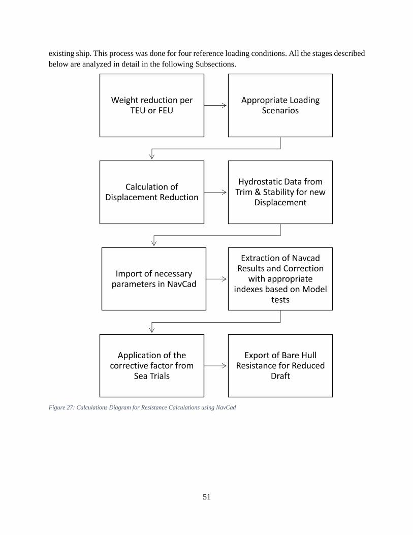
51

existing ship. This process was done for four reference loading conditions. All the stages described

below are analyzed in detail in the following Subsections.

Figure 27: Calculations Diagram for Resistance Calculations using NavCad

Weight reduction per TEU or FEU

Appropriate Loading Scenarios

Calculation of Displacement Reduction

Hydrostatic Data from Trim & Stability for new

Displacement

Import of necessary parameters in NavCad

Extraction of Navcad Results and Correction

with appropriate indexes based on Model

tests

Application of the corrective factor from

Sea Trials

Export of Bare Hull Resistance for Reduced

Draft

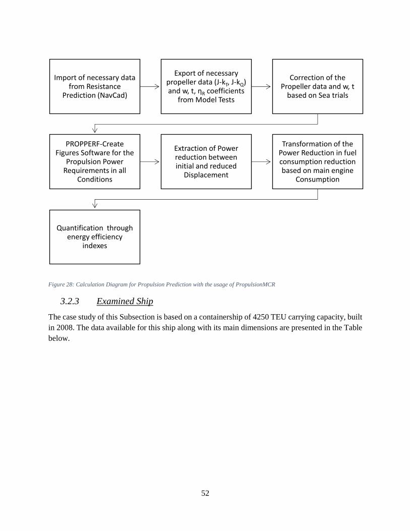
52

Figure 28: Calculation Diagram for Propulsion Prediction with the usage of PropulsionMCR

3.2.3 Examined Ship

The case study of this Subsection is based on a containership of 4250 TEU carrying capacity, built

in 2008. The data available for this ship along with its main dimensions are presented in the Table

below.

Import of necessary data from Resistance

Prediction (NavCad)

Export of necessary propeller data (J-kT, J-kQ) and w, t, ηR coefficients

from Model Tests

Correction of the Propeller data and w, t

based on Sea trials

PROPPERF-Create Figures Software for the

Propulsion Power Requirements in all

Conditions

Extraction of Power reduction between initial and reduced

Displacement

Transformation of the Power Reduction in fuel consumption reduction based on main engine

Consumption

Quantification through energy efficiency

indexes

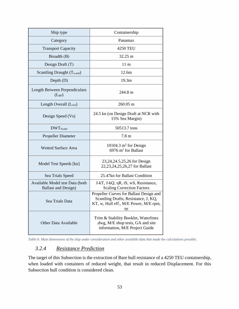
53

Ship type Containership

Category Panamax

Transport Capacity 4250 TEU

Breadth (Β) 32.25 m

Design Draft (Τ) 11 m

Scantling Draught (Tscantl) 12.6m

Depth (D) 19.3m

Length Between Perpendiculars

(LBP) 244.8 m

Length Overall (LOA) 260.05 m

Design Speed (Vs) 24.5 kn (on Design Draft at NCR with

15% Sea Margin)

DWTScantl 50513.7 tons

Propeller Diameter 7.8 m

Wetted Surface Area 10104.3 m2 for Design

6976 m2 for Ballast

Model Test Speeds [kn] 23,24,24.5,25,26 for Design

22,23,24,25,26,27 for Ballast

Sea Trials Speed 25.47kn for Ballast Condition

Available Model test Data (both

Ballast and Design)

J-kT, J-kQ, ηR, tS, wS, Resistance,

Scaling Correction Factors

Sea Trials Data

Propeller Curves for Ballast Design and

Scantling Drafts, Resistance, J, KQ,

KT, w, Hull eff., M/E Power, M/E rpm,

ηs

Other Data Available

Trim & Stability Booklet, Waterlines

.dwg, M/E shop tests, GA and site

information, M/E Project Guide

Table 6: Main dimensions of the ship under consideration and other available data that made the calculations possible.

3.2.4 Resistance Prediction

The target of this Subsection is the extraction of Bare hull resistance of a 4250 TEU containership,

when loaded with containers of reduced weight, that result in reduced Displacement. For this

Subsection hull condition is considered clean.

54

Containers made fully out of composite containers can be up to 78% lighter than their steel

counterparts. [48] Of course those very lightweight containers experience fatigue issues in stress

concentration areas such as the cube’s edges, where lashing equipment is attached. For this reason,

market available options, for the moment, use aluminum at those areas. Aluminum reinforced

containers weight 40% less than steel ones and are market available. [49]

Weight reduction is not the same when TEU or FEU are being loaded. TEU are more than half the

weight of FEU and thus loading TEU has increased tare weight and consequently higher reduction

potential. It is a fact that most containers shipped are FEU and the analogy is around 80% FEU

and 20% TEU. [59] For each loading scenario (fully TEU, fully FEU, realistic 20% TEU and 80%

FEU) the resulting weight reduction was calculated for both fully composite containers and

Composite Aluminum ones. The results are presented in Table 7 along with the Displacement

reduction from the Trim and Stability Manual of the 4250 TEU containership. Full FEU loading

values will not be a part of the rest of the calculations in this Section.

What is more, a quick prediction on the effect the weight reduction would have on Propulsion

Power of the ship was conducted using English Admiralty coefficient, as defined below. This

coefficient is unfortunately for new ship designs and provides an overestimation for draft reduction

cases of an already existing ship.

𝐶𝑁 =𝛥23∗𝑉3

𝑃, obviously Power is proportional to the displacement raised in the two thirds power

based on this formula, but the actual expected values are going to be lower, given the fact that the

ship is optimized for sailing at Design Draught.

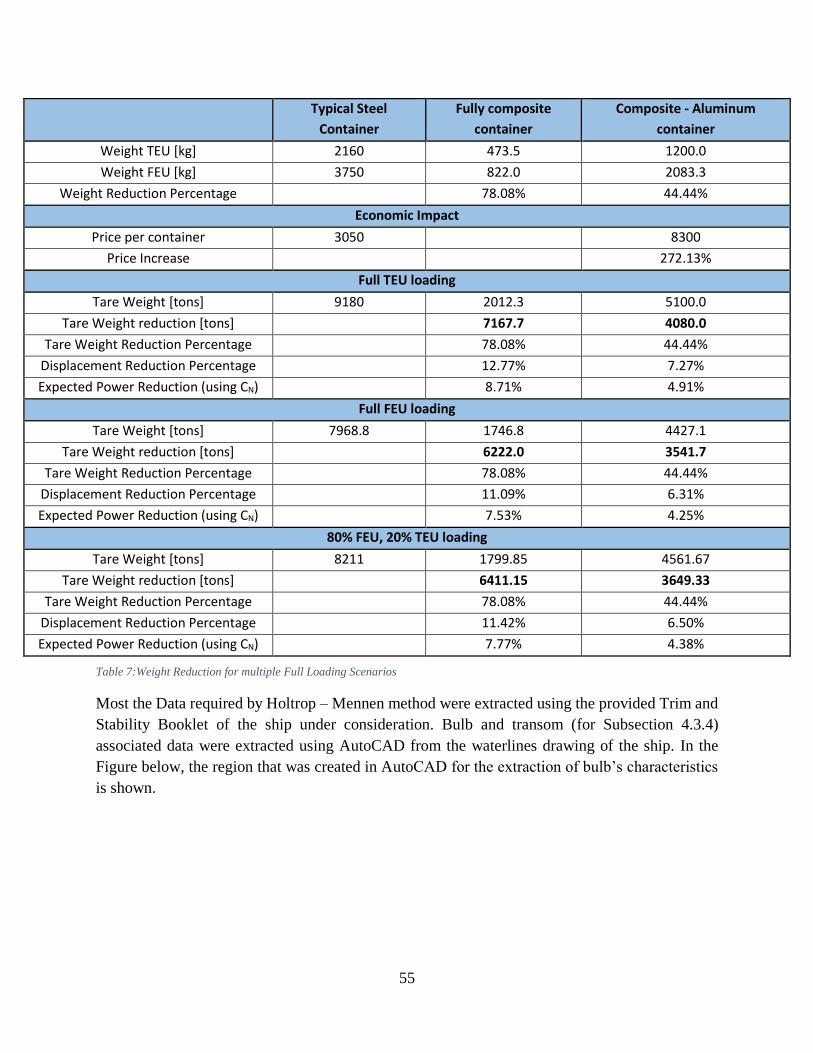
55

Table 7:Weight Reduction for multiple Full Loading Scenarios

Most the Data required by Holtrop – Mennen method were extracted using the provided Trim and

Stability Booklet of the ship under consideration. Bulb and transom (for Subsection 4.3.4)

associated data were extracted using AutoCAD from the waterlines drawing of the ship. In the

Figure below, the region that was created in AutoCAD for the extraction of bulb’s characteristics

is shown.

Typical Steel

Container

Fully composite

container

Composite - Aluminum

container

Weight TEU [kg] 2160 473.5 1200.0

Weight FEU [kg] 3750 822.0 2083.3

Weight Reduction Percentage 78.08% 44.44%

Economic Impact

Price per container 3050 8300

Price Increase 272.13%

Full TEU loading

Tare Weight [tons] 9180 2012.3 5100.0

Tare Weight reduction [tons] 7167.7 4080.0

Tare Weight Reduction Percentage 78.08% 44.44%

Displacement Reduction Percentage 12.77% 7.27%

Expected Power Reduction (using CN) 8.71% 4.91%

Full FEU loading

Tare Weight [tons] 7968.8 1746.8 4427.1

Tare Weight reduction [tons] 6222.0 3541.7

Tare Weight Reduction Percentage 78.08% 44.44%

Displacement Reduction Percentage 11.09% 6.31%

Expected Power Reduction (using CN) 7.53% 4.25%

80% FEU, 20% TEU loading

Tare Weight [tons] 8211 1799.85 4561.67

Tare Weight reduction [tons] 6411.15 3649.33

Tare Weight Reduction Percentage 78.08% 44.44%

Displacement Reduction Percentage 11.42% 6.50%

Expected Power Reduction (using CN) 7.77% 4.38%

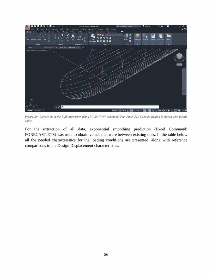
56

Figure 29: Extraction of the Bulb properties using MASSPROP command from AutoCAD. Created Region is shown with purple

color.

For the extraction of all data, exponential smoothing prediction (Excel Command:

FORECAST.ETS) was used to obtain values that were between existing ones. In the table below

all the needed characteristics for the loading conditions are presented, along with reference

comparisons to the Design Displacement characteristics.

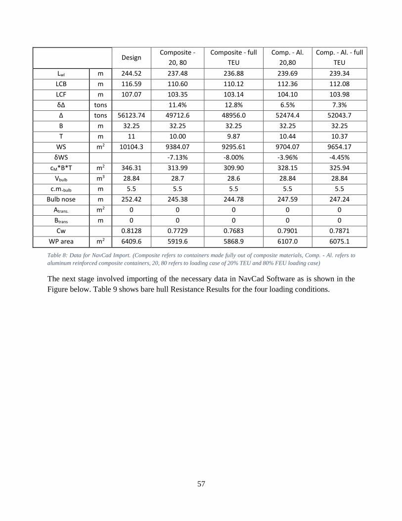
57

Design Composite -

20, 80

Composite - full

TEU

Comp. - Al.

20,80

Comp. - Al. - full

TEU

Lwl m 244.52 237.48 236.88 239.69 239.34

LCB m 116.59 110.60 110.12 112.36 112.08

LCF m 107.07 103.35 103.14 104.10 103.98

δΔ tons 11.4% 12.8% 6.5% 7.3%

Δ tons 56123.74 49712.6 48956.0 52474.4 52043.7

B m 32.25 32.25 32.25 32.25 32.25

T m 11 10.00 9.87 10.44 10.37

WS m2 10104.3 9384.07 9295.61 9704.07 9654.17

δWS -7.13% -8.00% -3.96% -4.45%

cM*B*T m2 346.31 313.99 309.90 328.15 325.94

Vbulb m3 28.84 28.7 28.6 28.84 28.84

c.m.bulb m 5.5 5.5 5.5 5.5 5.5

Bulb nose m 252.42 245.38 244.78 247.59 247.24

Atrans. m2 0 0 0 0 0

Btrans m 0 0 0 0 0

Cw 0.8128 0.7729 0.7683 0.7901 0.7871

WP area m2 6409.6 5919.6 5868.9 6107.0 6075.1

Table 8: Data for NavCad Import. (Composite refers to containers made fully out of composite materials, Comp. - Al. refers to

aluminum reinforced composite containers, 20, 80 refers to loading case of 20% TEU and 80% FEU loading case)

The next stage involved importing of the necessary data in NavCad Software as is shown in the

Figure below. Table 9 shows bare hull Resistance Results for the four loading conditions.

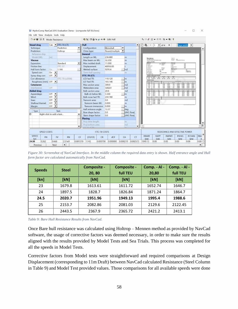
58

Figure 30: Screenshot of NavCad Interface. In the middle column the required data entry is shown. Half entrance angle and Hull

form factor are calculated automatically from NavCad.

Speeds Steel Composite -

20, 80

Composite -

full TEU

Comp. - Al -

20,80

Comp. - Al -

full TEU

[kn] [kN] [kN] [kN] [kN] [kN]

23 1679.8 1613.61 1611.72 1652.74 1646.7

24 1897.5 1828.7 1826.84 1871.24 1864.7

24.5 2020.7 1951.96 1949.13 1995.4 1988.6

25 2153.7 2082.86 2081.03 2129.6 2122.45

26 2443.5 2367.9 2365.72 2421.2 2413.1

Table 9: Bare Hull Resistance Results from NavCad.

Once Bare hull resistance was calculated using Holtrop – Mennen method as provided by NavCad

software, the usage of corrective factors was deemed necessary, in order to make sure the results

aligned with the results provided by Model Tests and Sea Trials. This process was completed for

all the speeds in Model Tests.

Corrective factors from Model tests were straightforward and required comparisons at Design

Displacement (corresponding to 11m Draft) between NavCad calculated Resistance (Steel Column

in Table 9) and Model Test provided values. Those comparisons for all available speeds were done

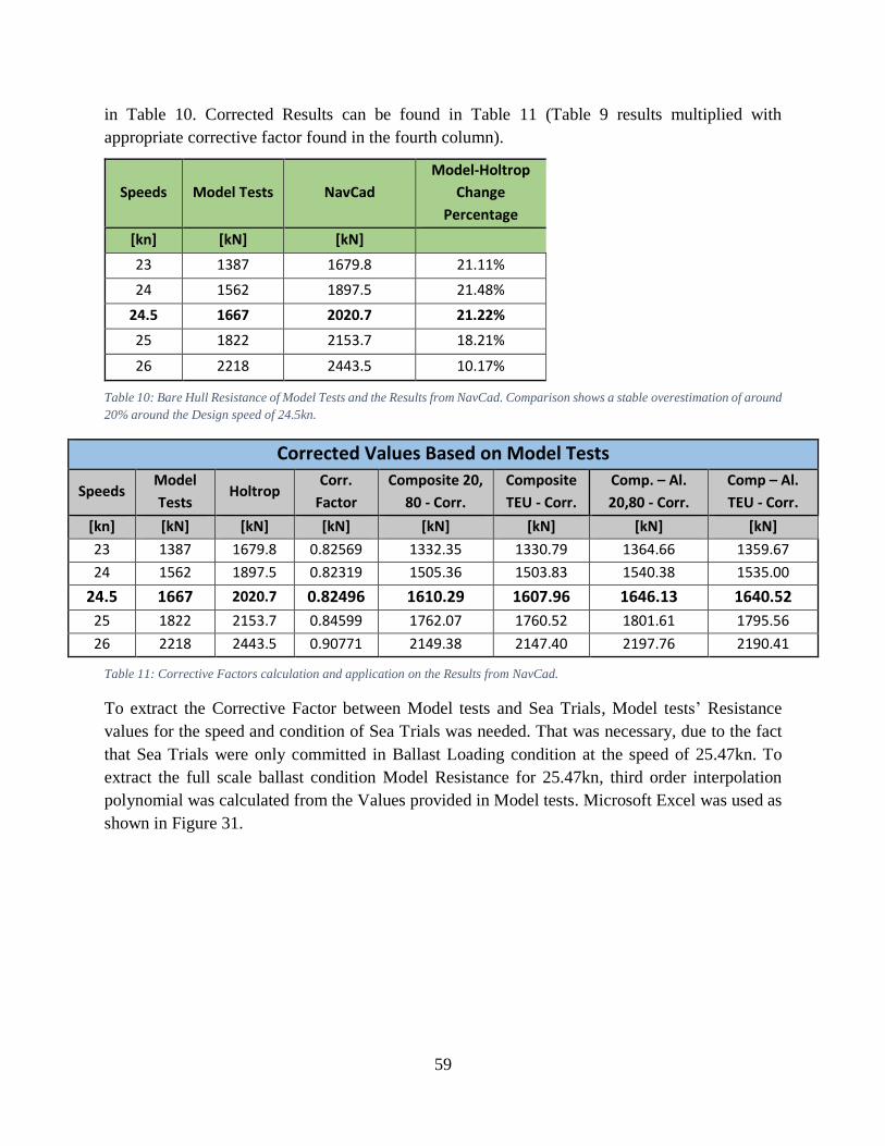
59

in Table 10. Corrected Results can be found in Table 11 (Table 9 results multiplied with

appropriate corrective factor found in the fourth column).

Speeds Model Tests NavCad

Model-Holtrop

Change

Percentage

[kn] [kN] [kN]

23 1387 1679.8 21.11%

24 1562 1897.5 21.48%

24.5 1667 2020.7 21.22%

25 1822 2153.7 18.21%

26 2218 2443.5 10.17%

Table 10: Bare Hull Resistance of Model Tests and the Results from NavCad. Comparison shows a stable overestimation of around

20% around the Design speed of 24.5kn.

Corrected Values Based on Model Tests

Speeds Model

Tests Holtrop

Corr.

Factor

Composite 20,

80 - Corr.

Composite

TEU - Corr.

Comp. – Al.

20,80 - Corr.

Comp – Al.

TEU - Corr.

[kn] [kN] [kN] [kN] [kN] [kN] [kN] [kN]

23 1387 1679.8 0.82569 1332.35 1330.79 1364.66 1359.67

24 1562 1897.5 0.82319 1505.36 1503.83 1540.38 1535.00

24.5 1667 2020.7 0.82496 1610.29 1607.96 1646.13 1640.52

25 1822 2153.7 0.84599 1762.07 1760.52 1801.61 1795.56

26 2218 2443.5 0.90771 2149.38 2147.40 2197.76 2190.41

Table 11: Corrective Factors calculation and application on the Results from NavCad.

To extract the Corrective Factor between Model tests and Sea Trials, Model tests’ Resistance

values for the speed and condition of Sea Trials was needed. That was necessary, due to the fact

that Sea Trials were only committed in Ballast Loading condition at the speed of 25.47kn. To

extract the full scale ballast condition Model Resistance for 25.47kn, third order interpolation

polynomial was calculated from the Values provided in Model tests. Microsoft Excel was used as

shown in Figure 31.

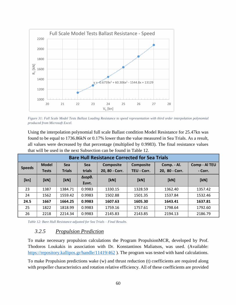
60

Figure 31: Full Scale Model Tests Ballast Loading Resistance to speed representation with third order interpolation polynomial

produced from Microsoft Excel.

Using the interpolation polynomial full scale Ballast condition Model Resistance for 25.47kn was

found to be equal to 1736.86kN or 0.17% lower than the value measured in Sea Trials. As a result,

all values were decreased by that percentage (multiplied by 0.9983). The final resistance values

that will be used in the next Subsection can be found in Table 12.

Bare Hull Resistance Corrected for Sea Trials

Speeds Model

Tests

Sea

Trials

Sea

trials

Composite

20, 80 - Corr.

Composite

TEU - Corr.

Comp. - Al.

20, 80 - Corr.

Comp - Al TEU

- Corr.

[kn] [kN] [kN] Διορθ.

Συντ. [kN] [kN] [kN] [kN]

23 1387 1384.71 0.9983 1330.15 1328.59 1362.40 1357.42

24 1562 1559.42 0.9983 1502.88 1501.35 1537.84 1532.46

24.5 1667 1664.25 0.9983 1607.63 1605.30 1643.41 1637.81

25 1822 1818.99 0.9983 1759.16 1757.61 1798.64 1792.60

26 2218 2214.34 0.9983 2145.83 2143.85 2194.13 2186.79

Table 12: Bare Hull Resistance adjusted for Sea Trials – Final Results.

3.2.5 Propulsion Prediction

To make necessary propulsion calculations the Program PropulsionMCR, developed by Prof.

Thodoros Loukakis in association with Dr. Konstantinos Maliatsos, was used. (Available:

https://repository.kallipos.gr/handle/11419/462 ). The program was tested with hand calculations.

To make Propulsion predictions wake (w) and thrust reduction (t) coefficients are required along

with propeller characteristics and rotation relative efficiency. All of these coefficients are provided

y = -0.6759x3 + 60.306x2 - 1544.8x + 13129

1000

1200

1400

1600

1800

2000

2200

20 21 22 23 24 25 26 27 28

RT

[kN

]

VS [kn]

Full Scale Model Tests Ballast Resistance - Speed

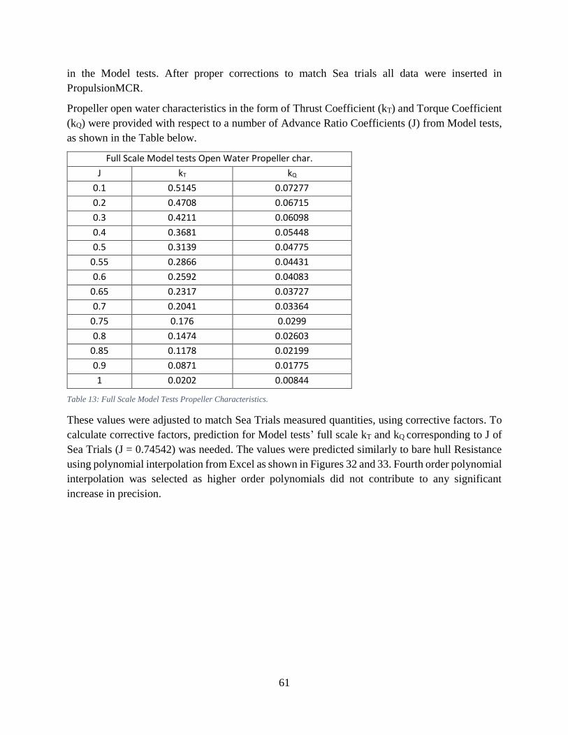
61

in the Model tests. After proper corrections to match Sea trials all data were inserted in

PropulsionMCR.

Propeller open water characteristics in the form of Thrust Coefficient (kT) and Torque Coefficient

(kQ) were provided with respect to a number of Advance Ratio Coefficients (J) from Model tests,

as shown in the Table below.

Full Scale Model tests Open Water Propeller char.

J kT kQ

0.1 0.5145 0.07277

0.2 0.4708 0.06715

0.3 0.4211 0.06098

0.4 0.3681 0.05448

0.5 0.3139 0.04775

0.55 0.2866 0.04431

0.6 0.2592 0.04083

0.65 0.2317 0.03727

0.7 0.2041 0.03364

0.75 0.176 0.0299

0.8 0.1474 0.02603

0.85 0.1178 0.02199

0.9 0.0871 0.01775

1 0.0202 0.00844

Table 13: Full Scale Model Tests Propeller Characteristics.

These values were adjusted to match Sea Trials measured quantities, using corrective factors. To

calculate corrective factors, prediction for Model tests’ full scale kT and kQ corresponding to J of

Sea Trials (J = 0.74542) was needed. The values were predicted similarly to bare hull Resistance

using polynomial interpolation from Excel as shown in Figures 32 and 33. Fourth order polynomial

interpolation was selected as higher order polynomials did not contribute to any significant

increase in precision.

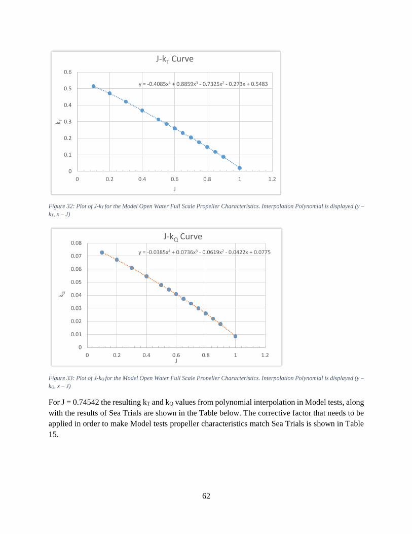
62

Figure 32: Plot of J-kT for the Model Open Water Full Scale Propeller Characteristics. Interpolation Polynomial is displayed (y –

kT, x – J)

Figure 33: Plot of J-kQ for the Model Open Water Full Scale Propeller Characteristics. Interpolation Polynomial is displayed (y –

kQ, x – J)

For J = 0.74542 the resulting kT and kQ values from polynomial interpolation in Model tests, along

with the results of Sea Trials are shown in the Table below. The corrective factor that needs to be

applied in order to make Model tests propeller characteristics match Sea Trials is shown in Table

15.

y = -0.4085x4 + 0.8859x3 - 0.7325x2 - 0.273x + 0.5483

0

0.1

0.2

0.3

0.4

0.5

0.6

0 0.2 0.4 0.6 0.8 1 1.2

k T

J

J-kT Curve

y = -0.0385x4 + 0.0736x3 - 0.0619x2 - 0.0422x + 0.0775

0

0.01

0.02

0.03

0.04

0.05

0.06

0.07

0.08

0 0.2 0.4 0.6 0.8 1 1.2

k Q

J

J-kQ Curve

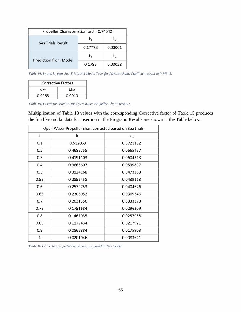
63

Propeller Characteristics for J = 0.74542

Sea Trials Result kT kQ

0.17778 0.03001

Prediction from Model kT kQ

0.1786 0.03028

Table 14: kT and kQ from Sea Trials and Model Tests for Advance Ratio Coefficient equal to 0.74542.

Corrective factors

δkT δkQ

0.9953 0.9910

Table 15: Corrective Factors for Open Water Propeller Characteristics.

Multiplication of Table 13 values with the corresponding Corrective factor of Table 15 produces

the final kT and kQ data for insertion in the Program. Results are shown in the Table below.

Open Water Propeller char. corrected based on Sea trials

J kT kQ

0.1 0.512069 0.0721152

0.2 0.4685755 0.0665457

0.3 0.4191103 0.0604313

0.4 0.3663607 0.0539897

0.5 0.3124168 0.0473203

0.55 0.2852458 0.0439113

0.6 0.2579753 0.0404626

0.65 0.2306052 0.0369346

0.7 0.2031356 0.0333373

0.75 0.1751684 0.0296309

0.8 0.1467035 0.0257958

0.85 0.1172434 0.0217921

0.9 0.0866884 0.0175903

1 0.0201046 0.0083641

Table 16:Corrected propeller characteristics based on Sea Trials.

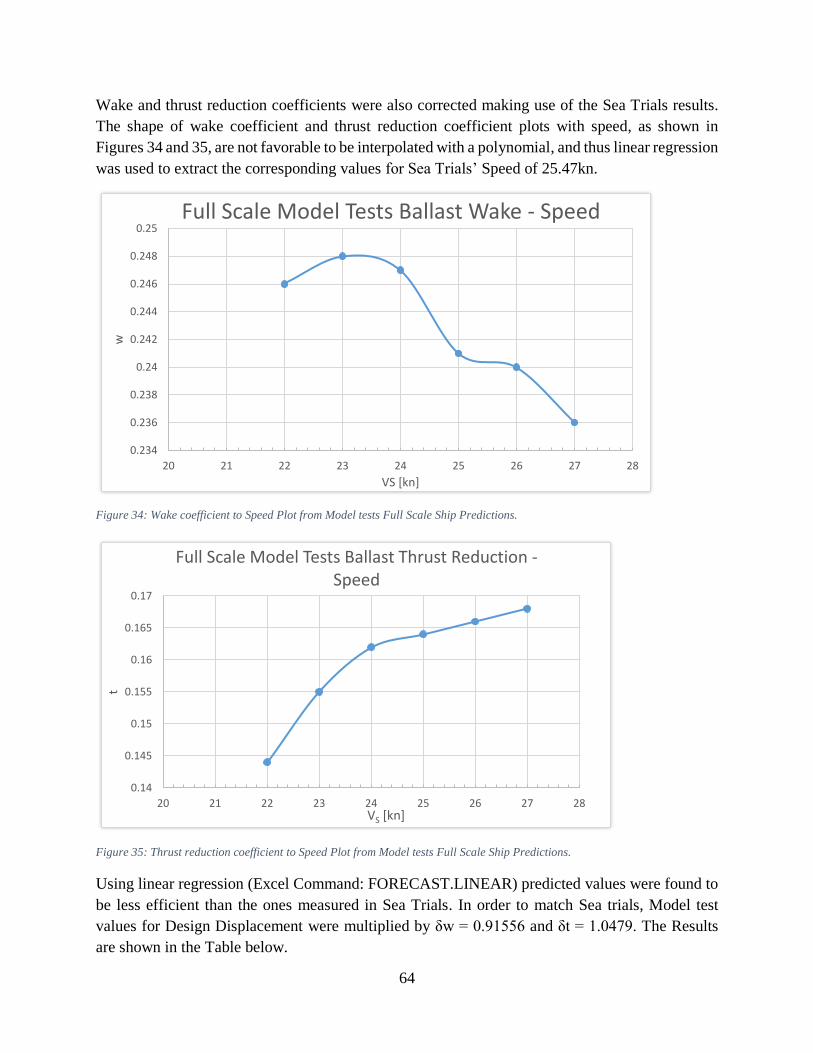
64

Wake and thrust reduction coefficients were also corrected making use of the Sea Trials results.

The shape of wake coefficient and thrust reduction coefficient plots with speed, as shown in

Figures 34 and 35, are not favorable to be interpolated with a polynomial, and thus linear regression

was used to extract the corresponding values for Sea Trials’ Speed of 25.47kn.

Figure 34: Wake coefficient to Speed Plot from Model tests Full Scale Ship Predictions.

Figure 35: Thrust reduction coefficient to Speed Plot from Model tests Full Scale Ship Predictions.

Using linear regression (Excel Command: FORECAST.LINEAR) predicted values were found to

be less efficient than the ones measured in Sea Trials. In order to match Sea trials, Model test

values for Design Displacement were multiplied by δw = 0.91556 and δt = 1.0479. The Results

are shown in the Table below.

0.234

0.236

0.238

0.24

0.242

0.244

0.246

0.248

0.25

20 21 22 23 24 25 26 27 28

w

VS [kn]

Full Scale Model Tests Ballast Wake - Speed

0.14

0.145

0.15

0.155

0.16

0.165

0.17

20 21 22 23 24 25 26 27 28

t

VS [kn]

Full Scale Model Tests Ballast Thrust Reduction -Speed

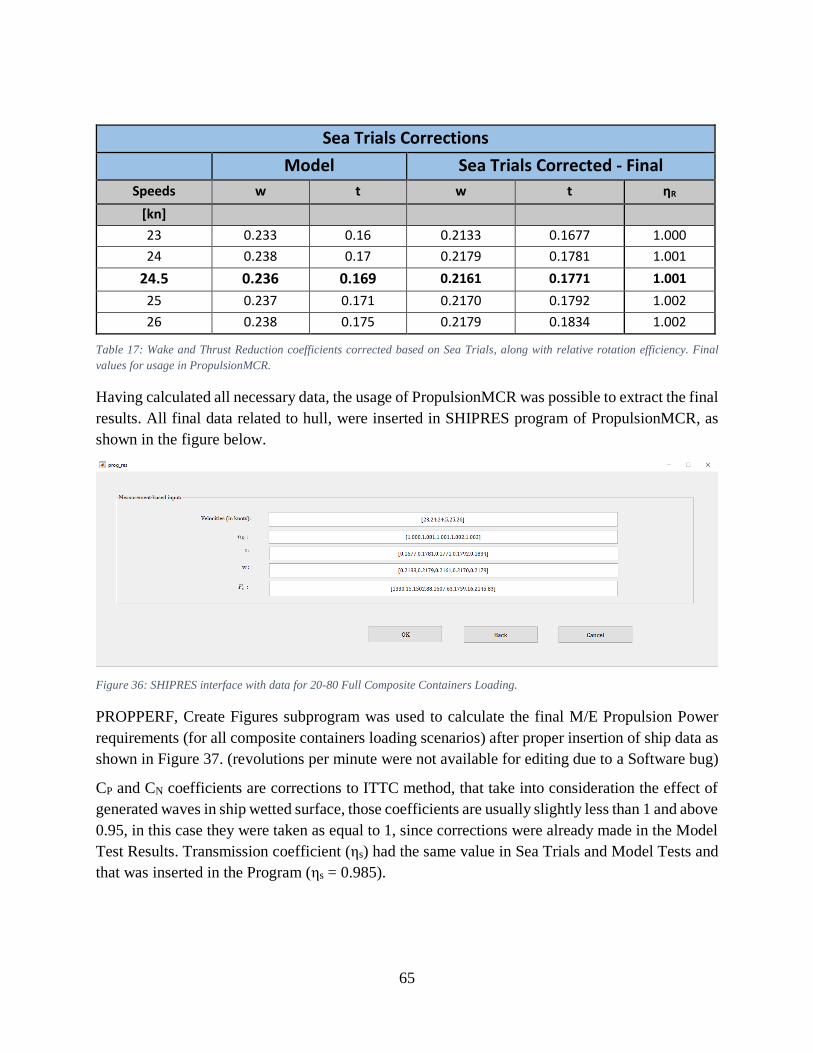
65

Sea Trials Corrections Model Sea Trials Corrected - Final

Speeds w t w t ηR

[kn]

23 0.233 0.16 0.2133 0.1677 1.000

24 0.238 0.17 0.2179 0.1781 1.001

24.5 0.236 0.169 0.2161 0.1771 1.001

25 0.237 0.171 0.2170 0.1792 1.002

26 0.238 0.175 0.2179 0.1834 1.002

Table 17: Wake and Thrust Reduction coefficients corrected based on Sea Trials, along with relative rotation efficiency. Final

values for usage in PropulsionMCR.

Having calculated all necessary data, the usage of PropulsionMCR was possible to extract the final

results. All final data related to hull, were inserted in SHIPRES program of PropulsionMCR, as

shown in the figure below.

Figure 36: SHIPRES interface with data for 20-80 Full Composite Containers Loading.

PROPPERF, Create Figures subprogram was used to calculate the final M/E Propulsion Power

requirements (for all composite containers loading scenarios) after proper insertion of ship data as

shown in Figure 37. (revolutions per minute were not available for editing due to a Software bug)

CP and CN coefficients are corrections to ITTC method, that take into consideration the effect of

generated waves in ship wetted surface, those coefficients are usually slightly less than 1 and above

0.95, in this case they were taken as equal to 1, since corrections were already made in the Model

Test Results. Transmission coefficient (ηs) had the same value in Sea Trials and Model Tests and

that was inserted in the Program (ηs = 0.985).

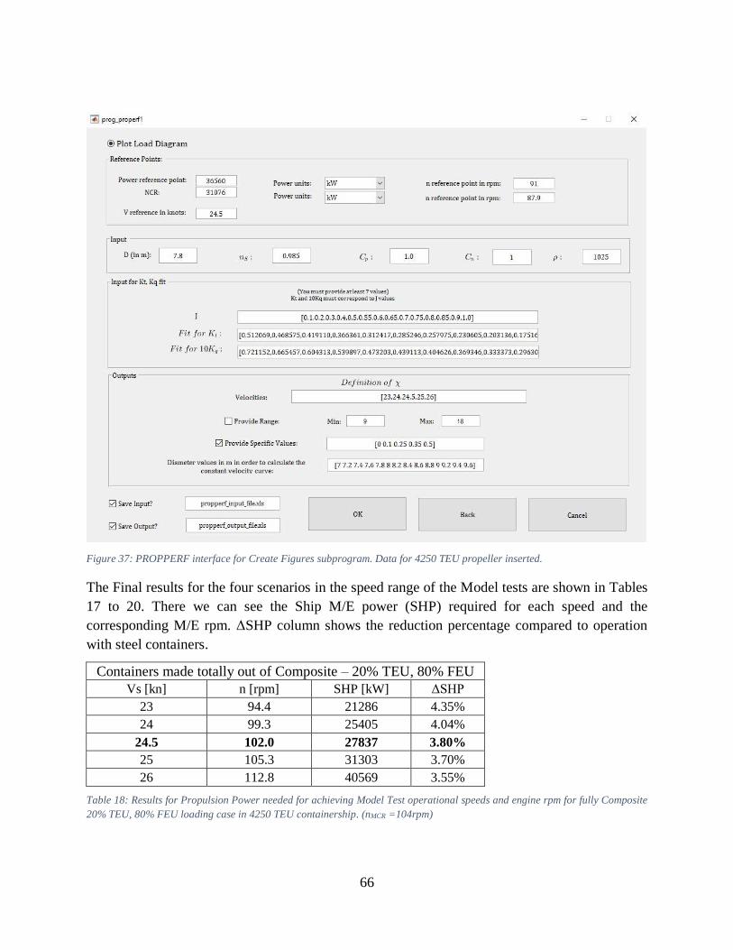
66

Figure 37: PROPPERF interface for Create Figures subprogram. Data for 4250 TEU propeller inserted.

The Final results for the four scenarios in the speed range of the Model tests are shown in Tables

17 to 20. There we can see the Ship M/E power (SHP) required for each speed and the

corresponding M/E rpm. ΔSHP column shows the reduction percentage compared to operation

with steel containers.

Containers made totally out of Composite – 20% TEU, 80% FEU

Vs [kn] n [rpm] SHP [kW] ΔSHP

23 94.4 21286 4.35%

24 99.3 25405 4.04%

24.5 102.0 27837 3.80%

25 105.3 31303 3.70%

26 112.8 40569 3.55%

Table 18: Results for Propulsion Power needed for achieving Model Test operational speeds and engine rpm for fully Composite

20% TEU, 80% FEU loading case in 4250 TEU containership. (nMCR =104rpm)

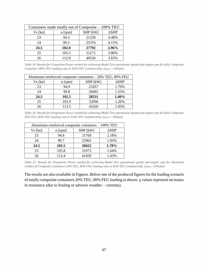
67

Containers made totally out of Composite – 100% TEU

Vs [kn] n [rpm] SHP [kW] ΔSHP

23 94.3 21258 4.48%

24 99.2 25376 4.15%

24.5 102.0 27792 3.96%

25 105.3 31272 3.80%

26 112.8 40526 3.65%

Table 19: Results for Propulsion Power needed for achieving Model Test operational speeds and engine rpm for fully Composite

Container 100% TEU loading case in 4250 TEU containership. (nMCR =104rpm)

Aluminum reinforced composite containers – 20% TEU, 80% FEU

Vs [kn] n [rpm] SHP [kW] ΔSHP

23 94.9 21857 1.79%

24 99.8 26065 1.55%

24.5 102.5 28531 1.40%

25 105.9 32096 1.26%

26 113.5 41620 1.05%

Table 20: Results for Propulsion Power needed for achieving Model Test operational speeds and engine rpm for fully Composite

20% TEU, 80% FEU loading case in 4250 TEU containership. (nMCR =104rpm)

Aluminum reinforced composite containers – 100% TEU

Vs [kn] n [rpm] SHP [kW] ΔSHP

23 94.8 21769 2.18%

24 99.7 25963 1.93%

24.5 102.5 28422 1.78%

25 105.8 31975 1.64%

26 113.4 41459 1.43%

Table 21: Results for Propulsion Power needed for achieving Model Test operational speeds and engine rpm for Aluminum

reinforced Composite Containers 20% TEU, 80% FEU loading case in 4250 TEU containership. (nMCR =104rpm)

The results are also available in Figures. Below one of the produced figures for the loading scenario

of totally composite containers 20% TEU, 80% FEU loading is shown. χ values represent increases

in resistance (due to fouling or adverse weather – currents).

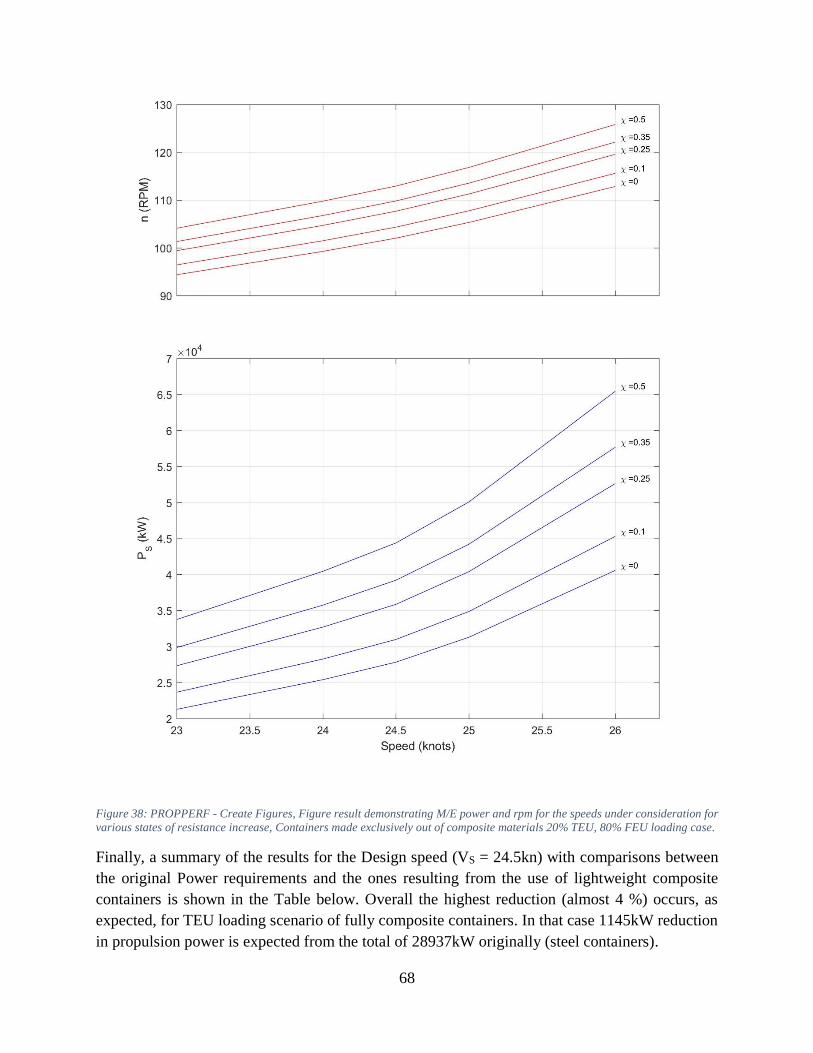
68

Figure 38: PROPPERF - Create Figures, Figure result demonstrating M/E power and rpm for the speeds under consideration for

various states of resistance increase, Containers made exclusively out of composite materials 20% TEU, 80% FEU loading case.

Finally, a summary of the results for the Design speed (VS = 24.5kn) with comparisons between

the original Power requirements and the ones resulting from the use of lightweight composite

containers is shown in the Table below. Overall the highest reduction (almost 4 %) occurs, as

expected, for TEU loading scenario of fully composite containers. In that case 1145kW reduction

in propulsion power is expected from the total of 28937kW originally (steel containers).

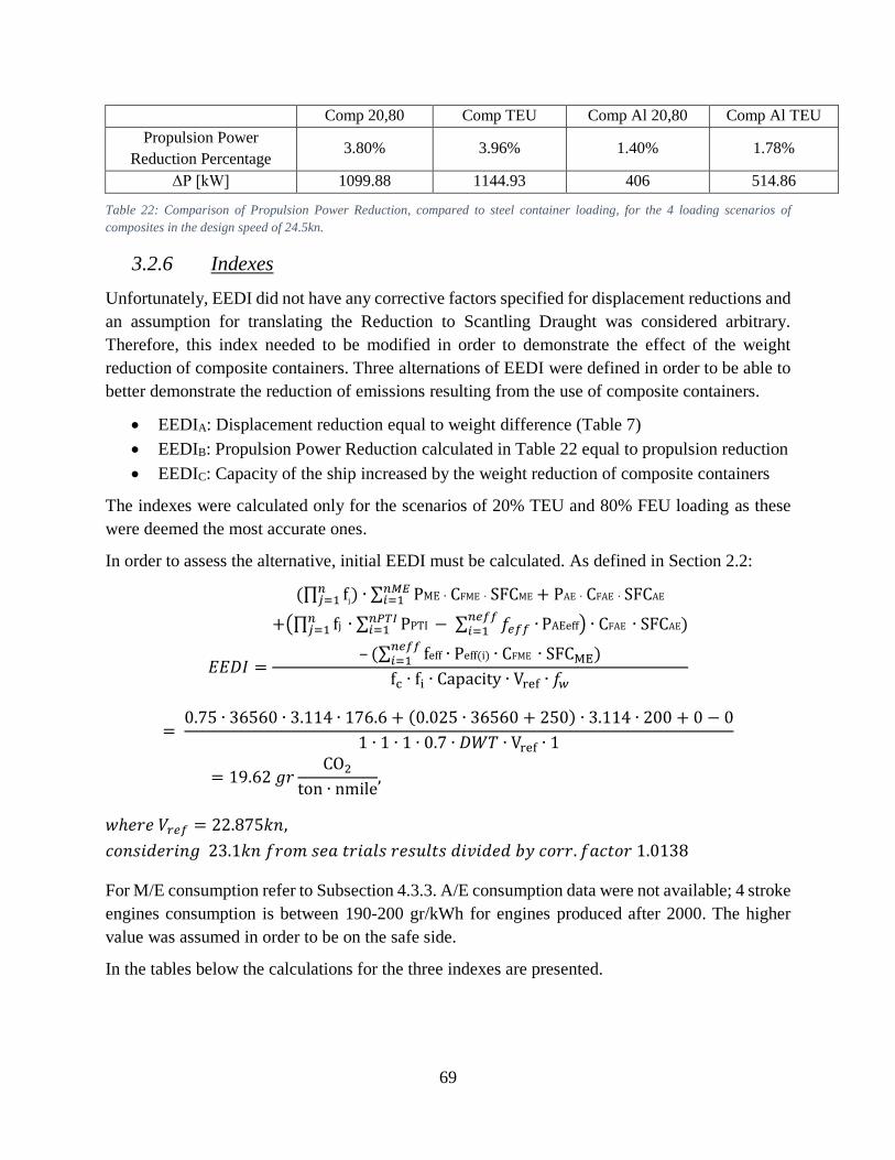
69

Comp 20,80 Comp TEU Comp Al 20,80 Comp Al TEU

Propulsion Power

Reduction Percentage 3.80% 3.96% 1.40% 1.78%

ΔP [kW] 1099.88 1144.93 406 514.86

Table 22: Comparison of Propulsion Power Reduction, compared to steel container loading, for the 4 loading scenarios of

composites in the design speed of 24.5kn.

3.2.6 Indexes

Unfortunately, EEDI did not have any corrective factors specified for displacement reductions and

an assumption for translating the Reduction to Scantling Draught was considered arbitrary.

Therefore, this index needed to be modified in order to demonstrate the effect of the weight

reduction of composite containers. Three alternations of EEDI were defined in order to be able to

better demonstrate the reduction of emissions resulting from the use of composite containers.

EEDIA: Displacement reduction equal to weight difference (Table 7)

EEDIB: Propulsion Power Reduction calculated in Table 22 equal to propulsion reduction

EEDIC: Capacity of the ship increased by the weight reduction of composite containers

The indexes were calculated only for the scenarios of 20% TEU and 80% FEU loading as these

were deemed the most accurate ones.

In order to assess the alternative, initial EEDI must be calculated. As defined in Section 2.2:

𝐸𝐸𝐷𝐼 =

(∏ fj) ∙ ∑ PME ∙ CFME ∙ SFCME𝑛𝑀𝐸𝑖=1

𝑛𝑗=1 + PAE ∙ CFAE ∙ SFCAE

+(∏ fj ∙ ∑ PPTI − ∑ 𝑓𝑒𝑓𝑓 ∙𝑛𝑒𝑓𝑓𝑖=1

𝑛𝑃𝑇𝐼𝑖=1 PAEeff𝑛

𝑗=1 ) ∙ CFAE ∙ SFCAE)

– (∑ feff ∙ Peff(i) ∙ CFME ∙ SFCME𝑛𝑒𝑓𝑓𝑖=1 )

fc ∙ fi ∙ Capacity ∙ Vref ∙ 𝑓𝑤

= 0.75 ∙ 36560 ∙ 3.114 ∙ 176.6 + (0.025 ∙ 36560 + 250) ∙ 3.114 ∙ 200 + 0 − 0

1 ∙ 1 ∙ 1 ∙ 0.7 ∙ 𝐷𝑊𝑇 ∙ Vref ∙ 1

= 19.62 𝑔𝑟CO2

ton ∙ nmile,

𝑤ℎ𝑒𝑟𝑒 𝑉𝑟𝑒𝑓 = 22.875𝑘𝑛,

𝑐𝑜𝑛𝑠𝑖𝑑𝑒𝑟𝑖𝑛𝑔 23.1𝑘𝑛 𝑓𝑟𝑜𝑚 𝑠𝑒𝑎 𝑡𝑟𝑖𝑎𝑙𝑠 𝑟𝑒𝑠𝑢𝑙𝑡𝑠 𝑑𝑖𝑣𝑖𝑑𝑒𝑑 𝑏𝑦 𝑐𝑜𝑟𝑟. 𝑓𝑎𝑐𝑡𝑜𝑟 1.0138

For M/E consumption refer to Subsection 4.3.3. A/E consumption data were not available; 4 stroke

engines consumption is between 190-200 gr/kWh for engines produced after 2000. The higher

value was assumed in order to be on the safe side.

In the tables below the calculations for the three indexes are presented.

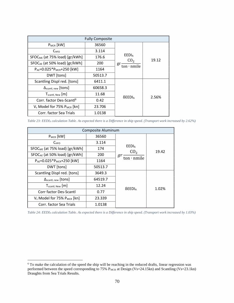
70

Fully Composite

PMCR [kW] 36560

EEDIA

grCO2

ton ∙ nmile

19.12

CHFO 3.114

SFOCME (at 75% load) [gr/kWh] 176.6

SFOCAE (at 50% load) [gr/kWh] 200

PAE=0.025*PMCR+250 [kW] 1164

DWT [tons] 50513.7

Scantling Displ red. [tons] 6411.1

δEEDIA 2.56%

Δscantl, new [tons] 60658.3

Tscantl, New [m] 11.68

Corr. factor Des-Scantl6 0.42

Vs Model for 75% PMCR [kn] 23.706

Corr. factor Sea Trials 1.0138

Table 23: EEDIA calculation Table. As expected there is a Difference in ship speed. (Transport work increased by 2.62%)

Composite Aluminum

PMCR [kW] 36560

EEDIA

𝑔𝑟CO2

ton ∙ nmile

19.42

CHFO 3.114

SFOCME (at 75% load) [gr/kWh] 174

SFOCAE (at 50% load) [gr/kWh] 200

PAE=0.025*PMCR+250 [kW] 1164

DWT [tons] 50513.7

Scantling Displ red. [tons] 3649.3

δEEDIA 1.02%

Δscantl, new [tons] 64519.7

Tscantl, New [m] 12.24

Corr factor Des-Scantl 0.77

Vs Model for 75% PMCR [kn] 23.339

Corr. factor Sea Trials 1.0138

Table 24: EEDIA calculation Table. As expected there is a Difference in ship speed. (Transport work increased by 1.03%)

6 To make the calculation of the speed the ship will be reaching in the reduced drafts, linear regression was

performed between the speed corresponding to 75% PMCR at Design (Vs=24.15kn) and Scantling (Vs=23.1kn)

Draughts from Sea Trials Results.

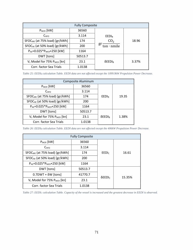
71

Fully Composite

PMCR [kW] 36560

EEDIB

grCO2

ton ∙ nmile

18.96

CHFO 3.114

SFOCME (at 75% load) [gr/kWh] 174

SFOCAE (at 50% load) [gr/kWh] 200

PAE=0.025*PMCR+250 [kW] 1164

DWT [tons] 50513.7

δEEDIB 3.37% Vs Model for 75% PMCR [kn] 23.1

Corr. factor Sea Trials 1.0138

Table 25: EEDIB calculation Table. EEDI data are not affected except the 1099.9kW Propulsion Power Decrease.

Composite Aluminum

PMCR [kW] 36560

EEDIB 19.35

CHFO 3.114

SFOCME (at 75% load) [gr/kWh] 174

SFOCAE (at 50% load) [gr/kWh] 200

PAE=0.025*PMCR+250 [kW] 1164

DWT [tons] 50513.7

δEEDIB 1.38% Vs Model for 75% PMCR [kn] 23.1

Corr. factor Sea Trials 1.0138

Table 26: EEDIB calculation Table. EEDI data are not affected except the 406kW Propulsion Power Decrease.

Fully Composite

PMCR [kW] 36560

EEDIC 16.61

CHFO 3.114

SFOCME (at 75% load) [gr/kWh] 174

SFOCAE (at 50% load) [gr/kWh] 200

PAE=0.025*PMCR+250 [kW] 1164

DWT [tons] 50513.7

δEEDIC 15.35% 0.7DWT + δW [tons] 41770.7

Vs Model for 75% PMCR [kn] 23.1

Corr. factor Sea Trials 1.0138

Table 27: EEDIC calculation Table. Capacity of the vessel is increased and the greatest decrease in EEDI is observed.

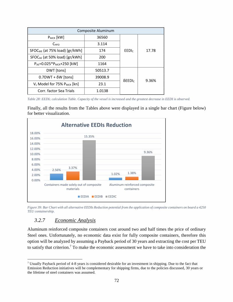
72

Composite Aluminum

PMCR [kW] 36560

EEDIC 17.78

CHFO 3.114

SFOCME (at 75% load) [gr/kWh] 174

SFOCAE (at 50% load) [gr/kWh] 200

PAE=0.025*PMCR+250 [kW] 1164

DWT [tons] 50513.7

δEEDIC 9.36% 0.7DWT + δW [tons] 39008.9

Vs Model for 75% PMCR [kn] 23.1

Corr. factor Sea Trials 1.0138

Table 28: EEDIC calculation Table. Capacity of the vessel is increased and the greatest decrease in EEDI is observed.

Finally, all the results from the Tables above were displayed in a single bar chart (Figure below)

for better visualization.

Figure 39: Bar Chart with all alternative EEDIs Reduction potential from the application of composite containers on board a 4250

TEU containership.

3.2.7 Economic Analysis

Aluminum reinforced composite containers cost around two and half times the price of ordinary

Steel ones. Unfortunately, no economic data exist for fully composite containers, therefore this

option will be analyzed by assuming a Payback period of 30 years and extracting the cost per TEU

to satisfy that criterion.7 To make the economic assessment we have to take into consideration the

7 Usually Payback period of 4-8 years is considered desirable for an investment in shipping. Due to the fact that

Emission Reduction initiatives will be complementary for shipping firms, due to the policies discussed, 30 years or

the lifetime of steel containers was assumed.

2.56%1.02%

3.37%

1.38%

15.35%

9.36%

0.00%

2.00%

4.00%

6.00%

8.00%

10.00%

12.00%

14.00%

16.00%

18.00%

Containers made solely out of compositematerials

Aluminum reinforced compositecontainers

Alternative EEDIs Reduction

EEDIA EEDIB EEDIC

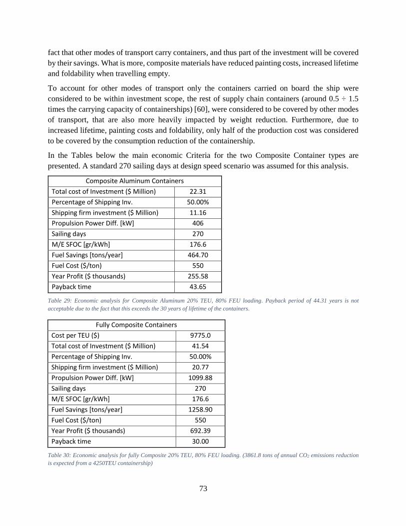
73

fact that other modes of transport carry containers, and thus part of the investment will be covered

by their savings. What is more, composite materials have reduced painting costs, increased lifetime

and foldability when travelling empty.

To account for other modes of transport only the containers carried on board the ship were

considered to be within investment scope, the rest of supply chain containers (around 0.5 ÷ 1.5

times the carrying capacity of containerships) [60], were considered to be covered by other modes

of transport, that are also more heavily impacted by weight reduction. Furthermore, due to

increased lifetime, painting costs and foldability, only half of the production cost was considered

to be covered by the consumption reduction of the containership.

In the Tables below the main economic Criteria for the two Composite Container types are

presented. A standard 270 sailing days at design speed scenario was assumed for this analysis.

Composite Aluminum Containers

Total cost of Investment ($ Million) 22.31

Percentage of Shipping Inv. 50.00%

Shipping firm investment ($ Million) 11.16

Propulsion Power Diff. [kW] 406

Sailing days 270

M/E SFOC [gr/kWh] 176.6

Fuel Savings [tons/year] 464.70

Fuel Cost ($/ton) 550

Year Profit ($ thousands) 255.58

Payback time 43.65

Table 29: Economic analysis for Composite Aluminum 20% TEU, 80% FEU loading. Payback period of 44.31 years is not

acceptable due to the fact that this exceeds the 30 years of lifetime of the containers.

Fully Composite Containers

Cost per TEU ($) 9775.0

Total cost of Investment ($ Million) 41.54

Percentage of Shipping Inv. 50.00%

Shipping firm investment ($ Million) 20.77

Propulsion Power Diff. [kW] 1099.88

Sailing days 270

M/E SFOC [gr/kWh] 176.6

Fuel Savings [tons/year] 1258.90

Fuel Cost ($/ton) 550

Year Profit ($ thousands) 692.39

Payback time 30.00

Table 30: Economic analysis for fully Composite 20% TEU, 80% FEU loading. (3861.8 tons of annual CO2 emissions reduction

is expected from a 4250TEU containership)

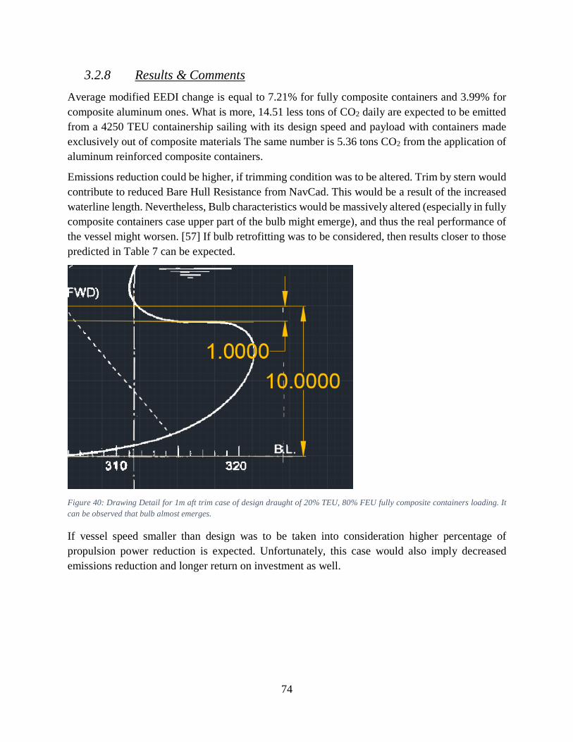
74

3.2.8 Results & Comments

Average modified EEDI change is equal to 7.21% for fully composite containers and 3.99% for

composite aluminum ones. What is more, 14.51 less tons of CO2 daily are expected to be emitted

from a 4250 TEU containership sailing with its design speed and payload with containers made

exclusively out of composite materials The same number is 5.36 tons CO2 from the application of

aluminum reinforced composite containers.

Emissions reduction could be higher, if trimming condition was to be altered. Trim by stern would

contribute to reduced Bare Hull Resistance from NavCad. This would be a result of the increased

waterline length. Nevertheless, Bulb characteristics would be massively altered (especially in fully

composite containers case upper part of the bulb might emerge), and thus the real performance of

the vessel might worsen. [57] If bulb retrofitting was to be considered, then results closer to those

predicted in Table 7 can be expected.

Figure 40: Drawing Detail for 1m aft trim case of design draught of 20% TEU, 80% FEU fully composite containers loading. It

can be observed that bulb almost emerges.

If vessel speed smaller than design was to be taken into consideration higher percentage of

propulsion power reduction is expected. Unfortunately, this case would also imply decreased

emissions reduction and longer return on investment as well.

75

3.3 Super Slow Steaming

Super slow steaming has recently been adopted by the majority of container shipping firms as a

means of coping with increased fuel rates and transporting vessel capacity oversupply. This

method is particularly successful in the container shipping industry, due to high design speeds of

its vessels. As already discussed in Section 3.7, this happens due to wave resistance, that implies

velocity reductions in high speeds result in cubic reductions in fuel consumption per ton mile,

compared to square ratio in slow speeds. For these reasons, it is not uncommon to see drops to

10% PMCR in this industry, with investments in retrofitting solutions (T/C cut out, PMI tuning,

Electronic Oil Lubricators, etc.) being a chartering benefit.

In order to make Super Slow steaming benefits more visible a case study was built for the 4250

TEU container ship, examined in the last Section. For ship information refer to Subsection 4.2.3.

The target of this Section will be the calculation of the resulting Speed for M/E operation at 5%

and 10% PMCR8. Once the speed is calculated the CII for Design Draft loading case will be

calculated and compared to operation at 25% PMCR and 75% PMCR. Also with respect to near future

EEXI regulation, compliance by means of Engine Power Limitation (EPL) will be examined and

the actual speed and power loss calculated. Weather issues were not analyzed for any of the loads

in this Section. EPL (Subsection 4.3.4) in particular, can be turned off by the crew in cases of

adverse weather and does not require additional attention. The same approach was taken as far

maneuverability is concerned, with extra caution by the crew being considered a safe method for

avoiding loss of control.

8 This is thought to be possible in all MAN electronic 2 stroke engines for prolonged periods according to Service

Letter SL2021-714/PXN. Available: https://www.man-es.com/docs/default-source/service-letters/sl2021-

714.pdf?sfvrsn=5279d333_4

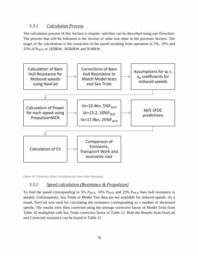
76

3.3.1 Calculation Process

The calculation process of this Section is simpler, and thus can be described using one flowchart.

The process that will be followed is the inverse of what was done in the previous Section. The

target of the calculations is the extraction of the speed resulting from operation in 5%, 10% and

25% of PMCR or 1828kW, 36560kW and 9140kW.

Figure 41: Flowchart of the Calculations for Super Slow Streaming.

3.3.2 Speed calculation (Resistance & Propulsion)

To find the speed corresponding to 5% PMCR, 10% PMCR and 25% PMCR bare hull resistance is

needed. Unfortunately, Sea Trials or Model Test data are not available for reduced speeds. As a

result, NavCad was used for calculating the resistance corresponding to a number of decreased

speeds. The results were then corrected using the average corrective factor of Model Tests from

Table 10 multiplied with Sea Trials corrective factor in Table 12. Both the Results from NavCad

and Corrected resistance can be found in Table 31.

Calculation of Bare Hull Resistance for

Reduced speeds using NavCad

Corrections of Bare Hull Resistance to Match Model tests

and Sea Trials

Assumptions for w, t, ηR coefficients for reduced speeds

Calculation of Power for each speed using

PropulsionMCR

Vs=10.4kn, 5%PMCR

Vs=13.2, 10%PMCR

Vs=17.9kn, 25%PMCR

M/E SFOC predictions

Calculation of CII

Comparison of Emissions,

Transprort Work and economic cost

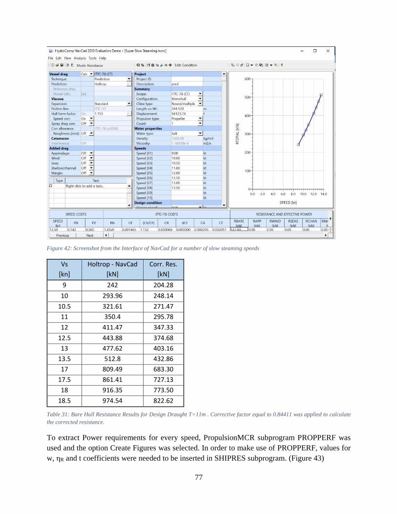
77

Figure 42: Screenshot from the Interface of NavCad for a number of slow steaming speeds

Vs

[kn]

Holtrop - NavCad

[kN]

Corr. Res.

[kN]

9 242 204.28

10 293.96 248.14

10.5 321.61 271.47

11 350.4 295.78

12 411.47 347.33

12.5 443.88 374.68

13 477.62 403.16

13.5 512.8 432.86

17 809.49 683.30

17.5 861.41 727.13

18 916.35 773.50

18.5 974.54 822.62

Table 31: Bare Hull Resistance Results for Design Draught T=11m . Corrective factor equal to 0.84411 was applied to calculate

the corrected resistance.

To extract Power requirements for every speed, PropulsionMCR subprogram PROPPERF was

used and the option Create Figures was selected. In order to make use of PROPPERF, values for

w, ηR and t coefficients were needed to be inserted in SHIPRES subprogram. (Figure 43)

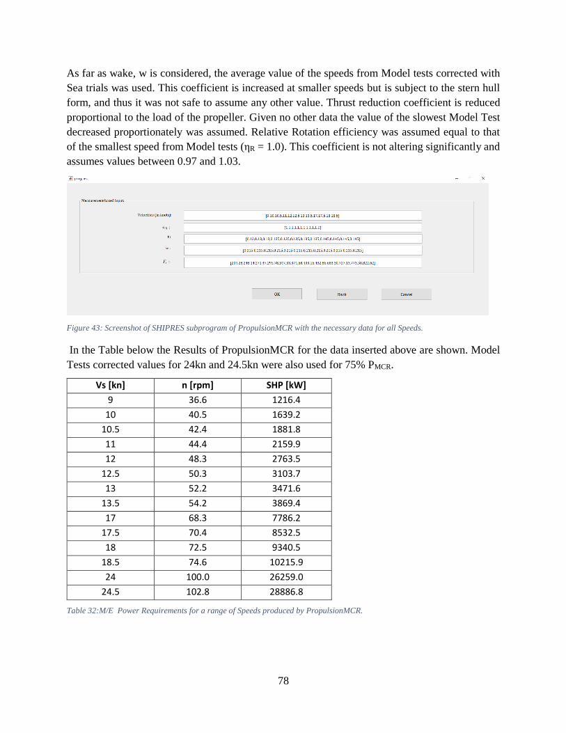
78

As far as wake, w is considered, the average value of the speeds from Model tests corrected with

Sea trials was used. This coefficient is increased at smaller speeds but is subject to the stern hull

form, and thus it was not safe to assume any other value. Thrust reduction coefficient is reduced

proportional to the load of the propeller. Given no other data the value of the slowest Model Test

decreased proportionately was assumed. Relative Rotation efficiency was assumed equal to that

of the smallest speed from Model tests (ηR = 1.0). This coefficient is not altering significantly and

assumes values between 0.97 and 1.03.

Figure 43: Screenshot of SHIPRES subprogram of PropulsionMCR with the necessary data for all Speeds.

In the Table below the Results of PropulsionMCR for the data inserted above are shown. Model

Tests corrected values for 24kn and 24.5kn were also used for 75% PMCR.

Vs [kn] n [rpm] SHP [kW]

9 36.6 1216.4

10 40.5 1639.2

10.5 42.4 1881.8

11 44.4 2159.9

12 48.3 2763.5

12.5 50.3 3103.7

13 52.2 3471.6

13.5 54.2 3869.4

17 68.3 7786.2

17.5 70.4 8532.5

18 72.5 9340.5

18.5 74.6 10215.9

24 100.0 26259.0

24.5 102.8 28886.8

Table 32:M/E Power Requirements for a range of Speeds produced by PropulsionMCR.

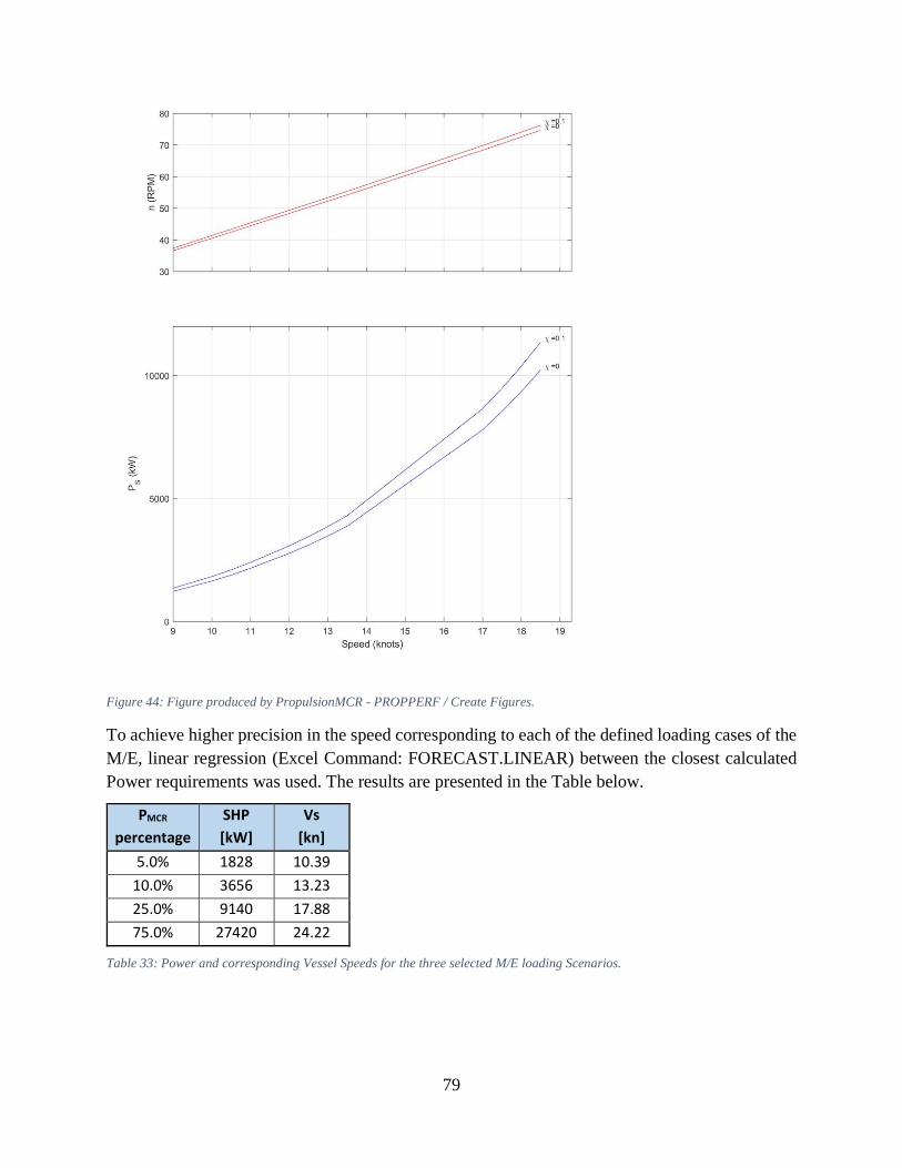
79

Figure 44: Figure produced by PropulsionMCR - PROPPERF / Create Figures.

To achieve higher precision in the speed corresponding to each of the defined loading cases of the

M/E, linear regression (Excel Command: FORECAST.LINEAR) between the closest calculated

Power requirements was used. The results are presented in the Table below.

PMCR

percentage

SHP

[kW]

Vs

[kn]

5.0% 1828 10.39

10.0% 3656 13.23

25.0% 9140 17.88

75.0% 27420 24.22

Table 33: Power and corresponding Vessel Speeds for the three selected M/E loading Scenarios.

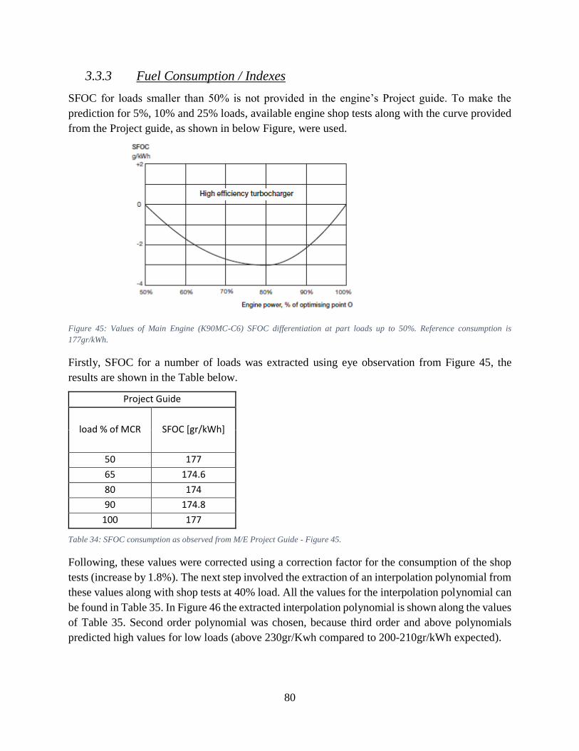
80

3.3.3 Fuel Consumption / Indexes

SFOC for loads smaller than 50% is not provided in the engine’s Project guide. To make the

prediction for 5%, 10% and 25% loads, available engine shop tests along with the curve provided

from the Project guide, as shown in below Figure, were used.

Figure 45: Values of Main Engine (K90MC-C6) SFOC differentiation at part loads up to 50%. Reference consumption is

177gr/kWh.

Firstly, SFOC for a number of loads was extracted using eye observation from Figure 45, the

results are shown in the Table below.

Project Guide

load % of MCR SFOC [gr/kWh]

50 177

65 174.6

80 174

90 174.8

100 177

Table 34: SFOC consumption as observed from M/E Project Guide - Figure 45.

Following, these values were corrected using a correction factor for the consumption of the shop

tests (increase by 1.8%). The next step involved the extraction of an interpolation polynomial from

these values along with shop tests at 40% load. All the values for the interpolation polynomial can

be found in Table 35. In Figure 46 the extracted interpolation polynomial is shown along the values

of Table 35. Second order polynomial was chosen, because third order and above polynomials

predicted high values for low loads (above 230gr/Kwh compared to 200-210gr/kWh expected).

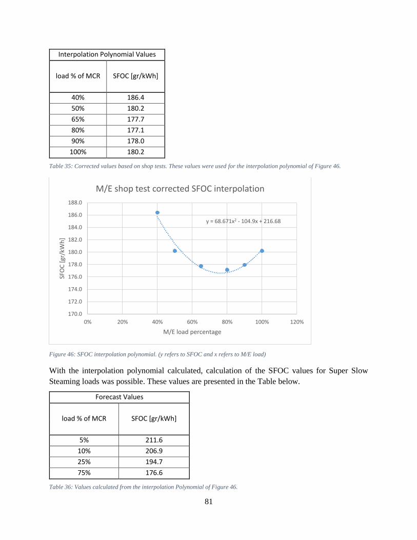
81

Interpolation Polynomial Values

load % of MCR SFOC [gr/kWh]

40% 186.4

50% 180.2

65% 177.7

80% 177.1

90% 178.0

100% 180.2

Table 35: Corrected values based on shop tests. These values were used for the interpolation polynomial of Figure 46.

Figure 46: SFOC interpolation polynomial. (y refers to SFOC and x refers to M/E load)

With the interpolation polynomial calculated, calculation of the SFOC values for Super Slow

Steaming loads was possible. These values are presented in the Table below.

Forecast Values

load % of MCR SFOC [gr/kWh]

5% 211.6

10% 206.9

25% 194.7

75% 176.6

Table 36: Values calculated from the interpolation Polynomial of Figure 46.

y = 68.671x2 - 104.9x + 216.68

170.0

172.0

174.0

176.0

178.0

180.0

182.0

184.0

186.0

188.0

0% 20% 40% 60% 80% 100% 120%

SFO

C [

gr/k

Wh

]

M/E load percentage

M/E shop test corrected SFOC interpolation

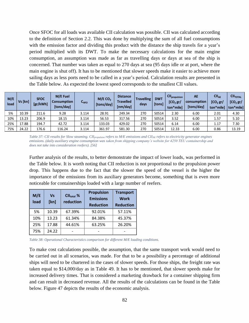
82

Once SFOC for all loads was available CII calculation was possible. CII was calculated according

to the definition of Section 2.2. This was done by multiplying the sum of all fuel consumptions

with the emission factor and dividing this product with the distance the ship travels for a year’s

period multiplied with its DWT. To make the necessary calculations for the main engine

consumption, an assumption was made as far as travelling days or days at sea of the ship is

concerned. That number was taken as equal to 270 days at sea (95 days idle or at port, where the

main engine is shut off). It has to be mentioned that slower speeds make it easier to achieve more

sailing days as less ports need to be called in a year’s period. Calculation results are presented in

the Table below. As expected the lowest speed corresponds to the smallest CII values.

Further analysis of the results, to better demonstrate the impact of lower loads, was performed in

the Table below. It is worth noting that CII reduction is not proportional to the propulsion power

drop. This happens due to the fact that the slower the speed of the vessel is the higher the

importance of the emissions from its auxiliary generators become, something that is even more

noticeable for containerships loaded with a large number of reefers.

M/E

load

Vs

[kn]

CIItotal %

reduction

Propulsion

Emissions

Reduction

Transport

Work

Reduction

5% 10.39 67.39% 92.01% 57.11%

10% 13.23 61.34% 84.38% 45.37%

25% 17.88 44.61% 63.25% 26.20%

75% 24.22 - - -

Table 38: Operational Characteristics comparison for different M/E loading conditions.

To make cost calculations possible, the assumption, that the same transport work would need to

be carried out in all scenarios, was made. For that to be a possibility a percentage of additional

ships will need to be chartered in the cases of slower speeds. For those ships, the freight rate was

taken equal to $14,000/day as in Table 49. It has to be mentioned, that slower speeds make for

increased delivery times. That is considered a marketing drawback for a container shipping firm

and can result in decreased revenue. All the results of the calculations can be found in the Table

below. Figure 47 depicts the results of the economic analysis.

Table 37: CII results for Slow steaming. CIIpropulsion refers to M/E emissions and CIIAE refers to electricity generator engines

emissions. (daily auxiliary engine consumption was taken from shipping company’s website for 4250 TEU containership and

does not take into consideration reefers). [56]

M/E

loadVs [kn]

SFOC

[gr/kWh]

M/E Fuel

Consumption

[tons/day]

CHFO

M/E CO2

[tons/day]

Distance

Travelled

[nm/day]

Travelling

days

DWT

[tons]

CIIpropulsion

[CO2 gr/

ton*mile]

AE

consumption

[tons/day]

CIIAE

[CO2 gr/

ton*mile]

CIITOTAL

[CO2 gr/

ton*mile]

5% 10.39 211.6 9.28 3.114 28.91 249.34 270 50514 2.30 6.00 2.01 4.30

10% 13.23 206.9 18.15 3.114 56.53 317.56 270 50514 3.52 6.00 1.57 5.10

25% 17.88 194.7 42.72 3.114 133.03 429.02 270 50514 6.14 6.00 1.17 7.30

75% 24.22 176.6 116.24 3.114 361.97 581.30 270 50514 12.33 6.00 0.86 13.19

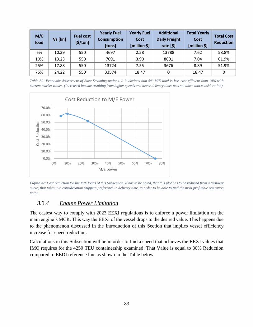
83

M/E

load Vs [kn]

Fuel cost

[$/ton]

Yearly Fuel

Consumption

[tons]

Yearly Fuel

Cost

[million $]

Additional

Daily Freight

rate [$]

Total Yearly

Cost

[million $]

Total Cost

Reduction

5% 10.39 550 4697 2.58 13788 7.62 58.8%

10% 13.23 550 7091 3.90 8601 7.04 61.9%

25% 17.88 550 13724 7.55 3676 8.89 51.9%

75% 24.22 550 33574 18.47 0 18.47 0

Table 39: Economic Assessment of Slow Steaming options. It is obvious that 5% M/E load is less cost-efficient than 10% with

current market values. (Increased income resulting from higher speeds and lower delivery times was not taken into consideration).

Figure 47: Cost reduction for the M/E loads of this Subsection. It has to be noted, that this plot has to be reduced from a turnover

curve, that takes into consideration shippers preference in delivery time, in order to be able to find the most profitable operation

point.

3.3.4 Engine Power Limitation

The easiest way to comply with 2023 EEXI regulations is to enforce a power limitation on the

main engine’s MCR. This way the EEXI of the vessel drops to the desired value. This happens due

to the phenomenon discussed in the Introduction of this Section that implies vessel efficiency

increase for speed reduction.

Calculations in this Subsection will be in order to find a speed that achieves the EEXI values that

IMO requires for the 4250 TEU containership examined. That Value is equal to 30% Reduction

compared to EEDI reference line as shown in the Table below.

0.0%

10.0%

20.0%

30.0%

40.0%

50.0%

60.0%

70.0%

0% 10% 20% 30% 40% 50% 60% 70% 80%

Co

st R

edu

ctio

n

M/E power

Cost Reduction to M/E Power

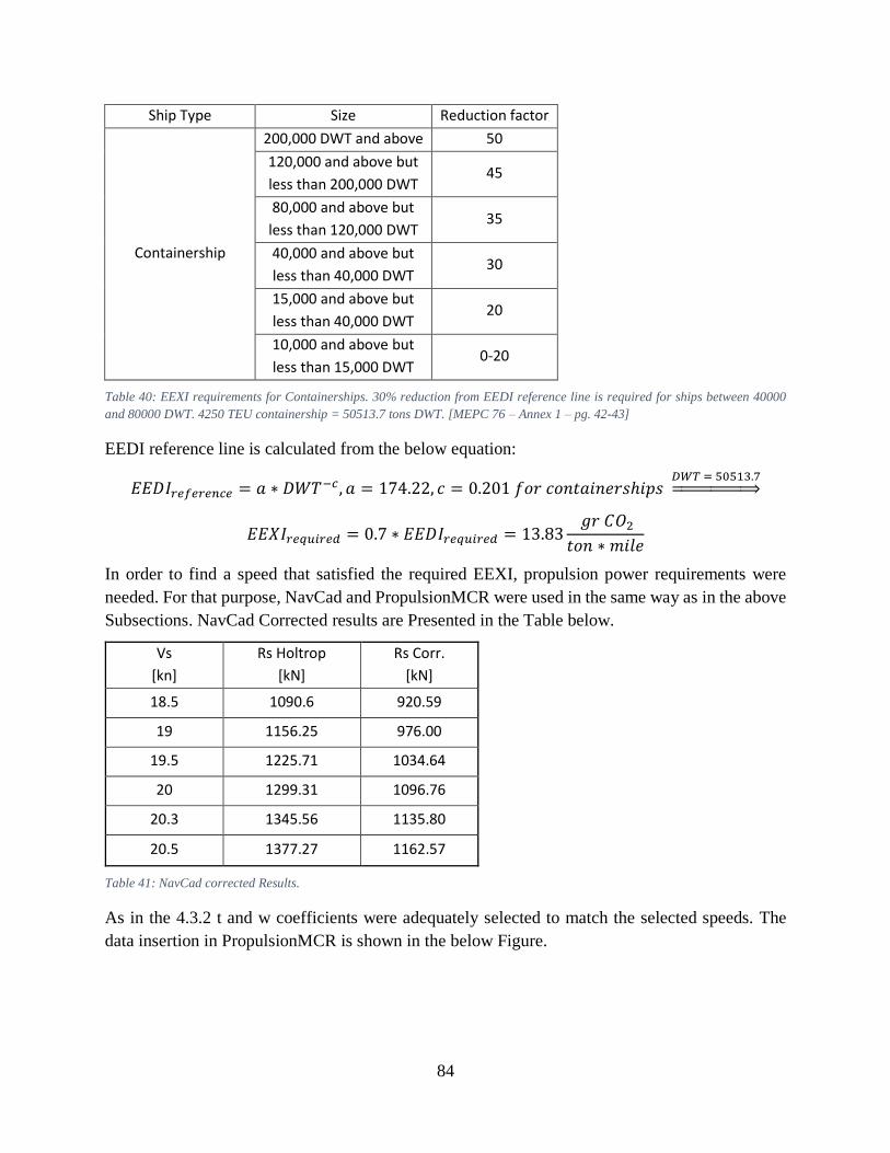
84

Ship Type Size Reduction factor

Containership

200,000 DWT and above 50

120,000 and above but

less than 200,000 DWT 45

80,000 and above but

less than 120,000 DWT 35

40,000 and above but

less than 40,000 DWT 30

15,000 and above but

less than 40,000 DWT 20

10,000 and above but

less than 15,000 DWT 0-20

Table 40: EEXI requirements for Containerships. 30% reduction from EEDI reference line is required for ships between 40000

and 80000 DWT. 4250 TEU containership = 50513.7 tons DWT. [MEPC 76 – Annex 1 – pg. 42-43]

EEDI reference line is calculated from the below equation:

𝐸𝐸𝐷𝐼𝑟𝑒𝑓𝑒𝑟𝑒𝑛𝑐𝑒 = 𝑎 ∗ 𝐷𝑊𝑇−𝑐, 𝑎 = 174.22, 𝑐 = 0.201 𝑓𝑜𝑟 𝑐𝑜𝑛𝑡𝑎𝑖𝑛𝑒𝑟𝑠ℎ𝑖𝑝𝑠

𝐷𝑊𝑇 = 50513.7⇒

𝐸𝐸𝑋𝐼𝑟𝑒𝑞𝑢𝑖𝑟𝑒𝑑 = 0.7 ∗ 𝐸𝐸𝐷𝐼𝑟𝑒𝑞𝑢𝑖𝑟𝑒𝑑 = 13.83 𝑔𝑟 𝐶𝑂2𝑡𝑜𝑛 ∗ 𝑚𝑖𝑙𝑒

In order to find a speed that satisfied the required EEXI, propulsion power requirements were

needed. For that purpose, NavCad and PropulsionMCR were used in the same way as in the above

Subsections. NavCad Corrected results are Presented in the Table below.

Vs

[kn]

Rs Holtrop

[kN]

Rs Corr.

[kN]

18.5 1090.6 920.59

19 1156.25 976.00

19.5 1225.71 1034.64

20 1299.31 1096.76

20.3 1345.56 1135.80

20.5 1377.27 1162.57

Table 41: NavCad corrected Results.

As in the 4.3.2 t and w coefficients were adequately selected to match the selected speeds. The

data insertion in PropulsionMCR is shown in the below Figure.

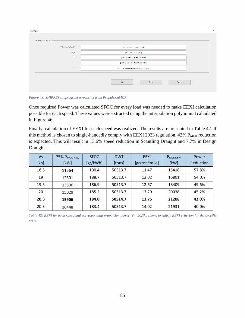
85

Figure 48: SHIPRES subprogram screenshot from PropulsionMCR

Once required Power was calculated SFOC for every load was needed to make EEXI calculation

possible for each speed. These values were extracted using the interpolation polynomial calculated

in Figure 46.

Finally, calculation of EEXI for each speed was realized. The results are presented in Table 42. If

this method is chosen to single-handedly comply with EEXI 2023 regulation, 42% PMCR reduction

is expected. This will result in 13.6% speed reduction in Scantling Draught and 7.7% in Design

Draught.

Vs

[kn]

75% PMCR, NEW

[kW]

SFOC

[gr/kWh]

DWT

[tons]

EEXI

[gr/ton*mile]

PMCR,NEW

[kW]

Power

Reduction

18.5 11564 190.4 50513.7 11.47 15418 57.8%

19 12601 188.7 50513.7 12.02 16801 54.0%

19.5 13806 186.9 50513.7 12.67 18409 49.6%

20 15029 185.2 50513.7 13.29 20038 45.2%

20.3 15906 184.0 50514.7 13.75 21208 42.0%

20.5 16448 183.4 50513.7 14.02 21931 40.0%

Table 42: EEXI for each speed and corresponding propulsion power. VS=20.3kn seems to satisfy EEXI criterion for the specific

vessel.

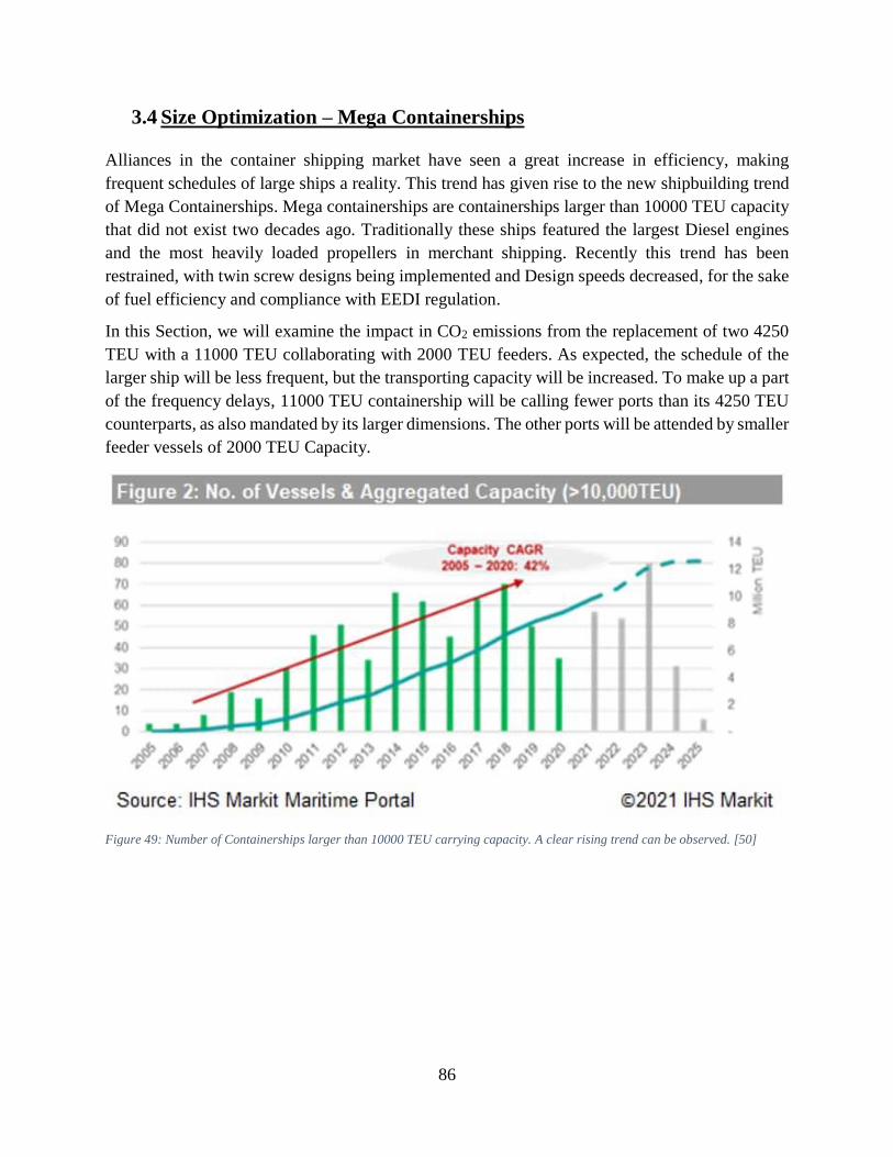
86

3.4 Size Optimization – Mega Containerships

Alliances in the container shipping market have seen a great increase in efficiency, making

frequent schedules of large ships a reality. This trend has given rise to the new shipbuilding trend

of Mega Containerships. Mega containerships are containerships larger than 10000 TEU capacity

that did not exist two decades ago. Traditionally these ships featured the largest Diesel engines

and the most heavily loaded propellers in merchant shipping. Recently this trend has been

restrained, with twin screw designs being implemented and Design speeds decreased, for the sake

of fuel efficiency and compliance with EEDI regulation.

In this Section, we will examine the impact in CO2 emissions from the replacement of two 4250

TEU with a 11000 TEU collaborating with 2000 TEU feeders. As expected, the schedule of the

larger ship will be less frequent, but the transporting capacity will be increased. To make up a part

of the frequency delays, 11000 TEU containership will be calling fewer ports than its 4250 TEU

counterparts, as also mandated by its larger dimensions. The other ports will be attended by smaller

feeder vessels of 2000 TEU Capacity.

Figure 49: Number of Containerships larger than 10000 TEU carrying capacity. A clear rising trend can be observed. [50]

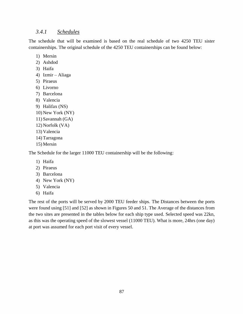
87

3.4.1 Schedules

The schedule that will be examined is based on the real schedule of two 4250 TEU sister

containerships. The original schedule of the 4250 TEU containerships can be found below:

1) Mersin

2) Ashdod

3) Haifa

4) Izmir – Aliaga

5) Piraeus

6) Livorno

7) Barcelona

8) Valencia

9) Halifax (NS)

10) New York (NY)

11) Savannah (GA)

12) Norfolk (VA)

13) Valencia

14) Tarragona

15) Mersin

The Schedule for the larger 11000 TEU containership will be the following:

1) Haifa

2) Piraeus

3) Barcelona

4) New York (NY)

5) Valencia

6) Haifa

The rest of the ports will be served by 2000 TEU feeder ships. The Distances between the ports

were found using [51] and [52] as shown in Figures 50 and 51. The Average of the distances from

the two sites are presented in the tables below for each ship type used. Selected speed was 22kn,

as this was the operating speed of the slowest vessel (11000 TEU). What is more, 24hrs (one day)

at port was assumed for each port visit of every vessel.

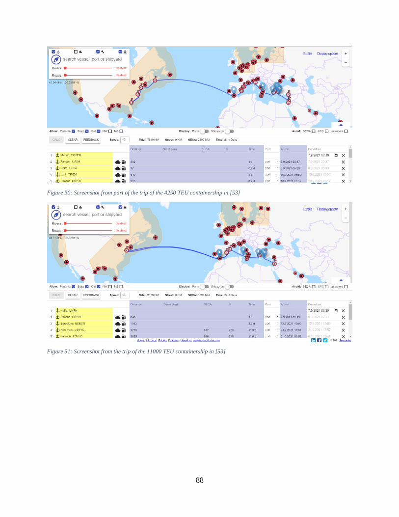
88

Figure 50: Screenshot from part of the trip of the 4250 TEU containership in [53]

Figure 51: Screenshot from the trip of the 11000 TEU containership in [53]

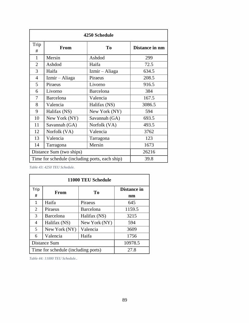
89

4250 Schedule

Trip

# From To Distance in nm

1 Mersin Ashdod 299

2 Ashdod Haifa 72.5

3 Haifa Izmir – Aliaga 634.5

4 Izmir – Aliaga Piraeus 208.5

5 Piraeus Livorno 916.5

6 Livorno Barcelona 384

7 Barcelona Valencia 167.5

8 Valencia Halifax (NS) 3086.5

9 Halifax (NS) New York (NY) 594

10 New York (NY) Savannah (GA) 693.5

11 Savannah (GA) Norfolk (VA) 493.5

12 Norfolk (VA) Valencia 3762

13 Valencia Tarragona 123

14 Tarragona Mersin 1673

Distance Sum (two ships) 26216

Time for schedule (including ports, each ship) 39.8

Table 43: 4250 TEU Schedule.

11000 TEU Schedule

Trip

# From To

Distance in

nm

1 Haifa Piraeus 645

2 Piraeus Barcelona 1159.5

3 Barcelona Halifax (NS) 3215

4 Halifax (NS) New York (NY) 594

5 New York (NY) Valencia 3609

6 Valencia Haifa 1756

Distance Sum 10978.5

Time for schedule (including ports) 27.8

Table 44: 11000 TEU Schedule..

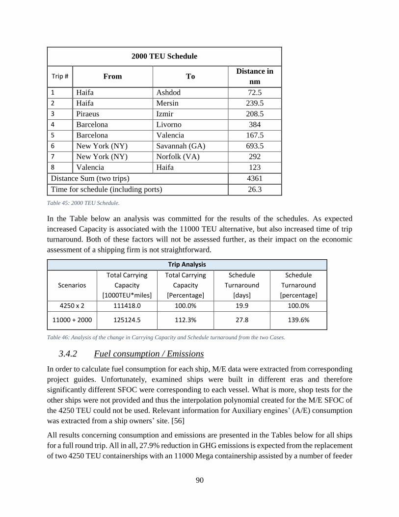
90

2000 TEU Schedule

Trip # From To Distance in

nm

1 Haifa Ashdod 72.5

2 Haifa Mersin 239.5

3 Piraeus Izmir 208.5

4 Barcelona Livorno 384

5 Barcelona Valencia 167.5

6 New York (NY) Savannah (GA) 693.5

7 New York (NY) Norfolk (VA) 292

8 Valencia Haifa 123

Distance Sum (two trips) 4361

Time for schedule (including ports) 26.3

Table 45: 2000 TEU Schedule.

In the Table below an analysis was committed for the results of the schedules. Αs expected

increased Capacity is associated with the 11000 TEU alternative, but also increased time of trip

turnaround. Both of these factors will not be assessed further, as their impact on the economic

assessment of a shipping firm is not straightforward.

Trip Analysis

Scenarios

Total Carrying

Capacity

[1000TEU*miles]

Total Carrying

Capacity

[Percentage]

Schedule

Turnaround

[days]

Schedule

Turnaround

[percentage]

4250 x 2 111418.0 100.0% 19.9 100.0%

11000 + 2000 125124.5 112.3% 27.8 139.6%

Table 46: Analysis of the change in Carrying Capacity and Schedule turnaround from the two Cases.

3.4.2 Fuel consumption / Emissions

In order to calculate fuel consumption for each ship, M/E data were extracted from corresponding

project guides. Unfortunately, examined ships were built in different eras and therefore

significantly different SFOC were corresponding to each vessel. What is more, shop tests for the

other ships were not provided and thus the interpolation polynomial created for the M/E SFOC of

the 4250 TEU could not be used. Relevant information for Auxiliary engines’ (A/E) consumption

was extracted from a ship owners’ site. [56]

All results concerning consumption and emissions are presented in the Tables below for all ships

for a full round trip. All in all, 27.9% reduction in GHG emissions is expected from the replacement

of two 4250 TEU containerships with an 11000 Mega containership assisted by a number of feeder

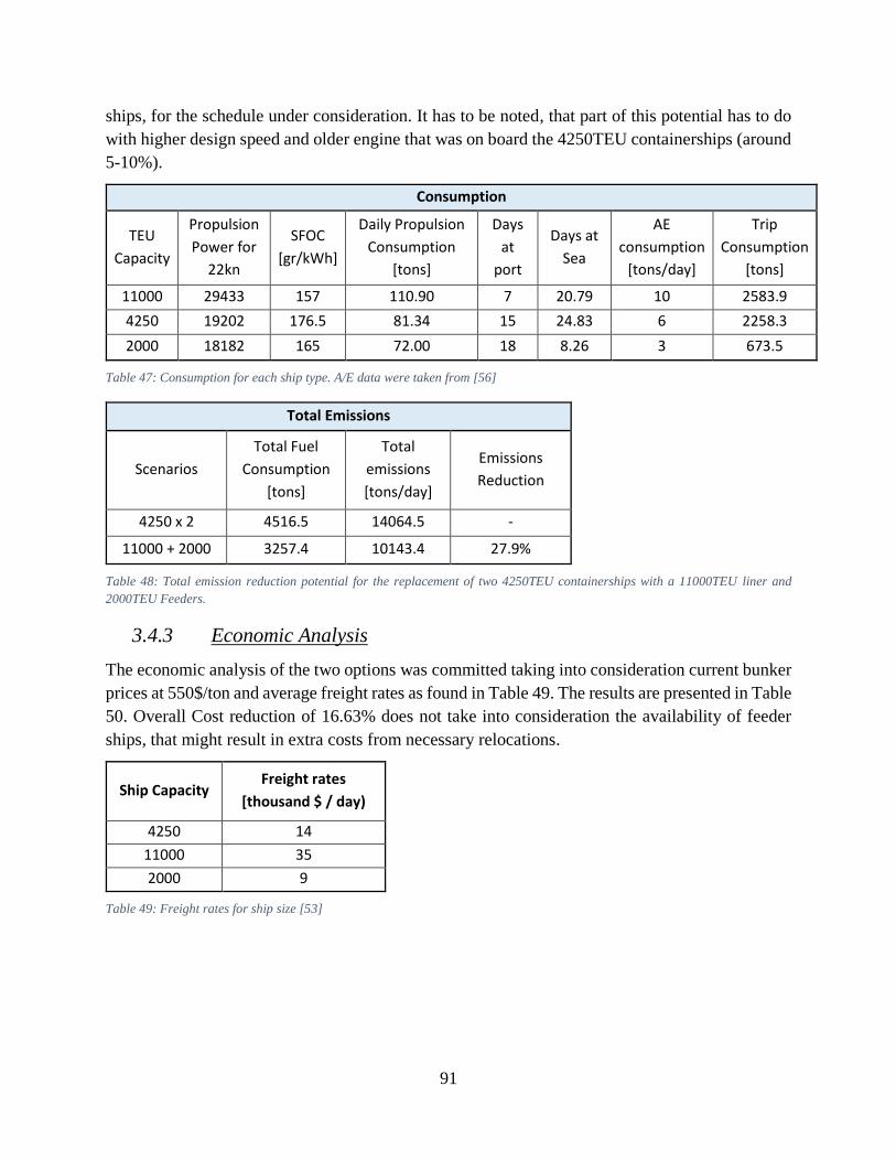
91

ships, for the schedule under consideration. It has to be noted, that part of this potential has to do

with higher design speed and older engine that was on board the 4250TEU containerships (around

5-10%).

Consumption

TEU

Capacity

Propulsion

Power for

22kn

SFOC

[gr/kWh]

Daily Propulsion

Consumption

[tons]

Days

at

port

Days at

Sea

AE

consumption

[tons/day]

Trip

Consumption

[tons]

11000 29433 157 110.90 7 20.79 10 2583.9

4250 19202 176.5 81.34 15 24.83 6 2258.3

2000 18182 165 72.00 18 8.26 3 673.5

Table 47: Consumption for each ship type. A/E data were taken from [56]

Total Emissions

Scenarios

Total Fuel

Consumption

[tons]

Total

emissions

[tons/day]

Emissions

Reduction

4250 x 2 4516.5 14064.5 -

11000 + 2000 3257.4 10143.4 27.9%

Table 48: Total emission reduction potential for the replacement of two 4250TEU containerships with a 11000TEU liner and

2000TEU Feeders.

3.4.3 Economic Analysis

The economic analysis of the two options was committed taking into consideration current bunker

prices at 550$/ton and average freight rates as found in Table 49. The results are presented in Table

50. Overall Cost reduction of 16.63% does not take into consideration the availability of feeder

ships, that might result in extra costs from necessary relocations.

Ship Capacity Freight rates

[thousand $ / day)

4250 14

11000 35

2000 9

Table 49: Freight rates for ship size [53]

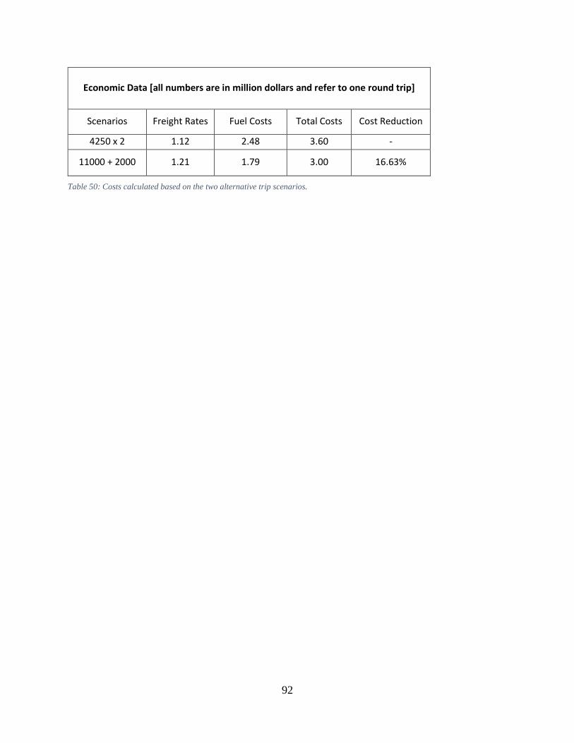
92

Economic Data [all numbers are in million dollars and refer to one round trip]

Scenarios Freight Rates Fuel Costs Total Costs Cost Reduction

4250 x 2 1.12 2.48 3.60 -

11000 + 2000 1.21 1.79 3.00 16.63%

Table 50: Costs calculated based on the two alternative trip scenarios.

93

3.5 Results Summary – Comparison

All things considered, the alternatives analyzed in this Chapter could be broken down into two

categories. In the first one the two types of Composite Containers can be included. The cost of

investment for those alternatives is significant and the resulting fuel cost reduction is not sufficient

for an acceptable investment Payback. In the second category, Super Slow Steaming and Mega

Containerships, require smaller investment and the resulting emissions and cost reductions are

significantly higher. The problem in those alternatives lies in the increased delivery time, resulting

from changes in the frequency or the travelling time of the schedule. This is a particularly

important parameter for the container shipping business, where cargo value is many times higher

than shipping costs.

Market conditions are very important for the evaluation of GHG emission alternatives. This Thesis

was committed at an era of increased chartering rates and bunker oil prices. The sailing day

scenario used in this thesis is quite optimistic. Frequent port calls of containerships, in this era of

port congestion, can result in reduced number of days at sea depending on the Schedule of the ship.

The indexes used for each case were different in order to better demonstrate the results of each

alternative. Below a Brief Summary of the results of the analyzed alternatives from this Chapter

can be found.

Alternative Capacity of

Ships in Case Study

Investment Cost (in $ Million)

ROI (in $ Million per

year)

Emissions Reduction Potential

Transport Work Reduction

Market Acceptance

Composite Aluminum Containers

4250 22.3125 0.256 3.92%

EEDIMODIFIED none small

Fully Composite Containers

4250 - 0.692 7.09%

EEDIMODIFIED none none

Super Slow Steaming 4250 - 10.850 67.4% CII 57.1% high

Engine Power Limitation

4250 - - 29.9% EEDI 13.6% in Scantling

7.7% in Design mandatory from 2023

Mega Containerships 4250, 2000, 11000

- 15.9% total

cost reduction 27% total emissions

12.3% increase in Capacity

39.6% decrease in schedule frequency

high

Table 51: Results summary of all the Case Studies in Chapter 4.

94

4. Conclusions – Suggestions for Further Studies

All things considered, there are many alternatives available to achieve the targets set by IMO for

2050. It can be argued as to whether these targets are austere enough to combat Greenhouse Gas

effects, but this thesis has clearly demonstrated that there are a lot of alternatives, that if combined,

can lower the emissions to levels even lower than the ones required by the IMO for the coming

years.

Investments in GHG reduction alternatives require prediction of the reduction potential in order to

make a proper assessment. This potential is affected by vessel-specific operational parameters. It

comes to no surprise, therefore that in order to select an alternative that is most efficient for a ship,

vessel-specific analysis is required. In my thesis, I have tried to uncover the vessel-specific

potential for three of those alternatives, composite containers, slow steaming and Size utilization

from the usage of Mega Containerships. The results and further research suggestions for these

alternatives, along with the ones briefly analyzed in Chapter 3, are summarized below.

Alternatives Review: Many alternatives exist as retrofitting or design options. Almost total

decarbonization can be achieved by available alternatives. Some alternatives are even cost efficient

for the amount of fuel they save.

Further Study:

Interaction between different alternatives (efficiency for the installation of more than one

alternative on board) and ship type.

Study on the feasibility of CC implementation on large merchant ship.

Composite Containers: Containers made fully out of composite containers are still under

development and can be up to 78% lighter than their steel counterparts. Aluminum reinforced

containers weight 40% less than steel ones and are market available. For reduced displacement

resulting from reduced containers weight, calculations were made to determine new resistance and

new propulsion power requirements. Around 4% propulsion power and subsequently ship

emissions reduction is expected from fully composite containers without any other operational

parameter modifications. That percentage drops to 1.5% for Aluminum reinforced composite

containers. Investment required is around 15% of a ship’s building price, taking into consideration

other forms of transport are also benefitted and reduced OPEX is expected from decreased painting

and increased lifetime. IMO EEDI index was properly altered to take into consideration tare weight

reductions in order to asses this alternative. Average modified EEDI reduction is equal to 7.21%

for fully composite containers and 3.99% for composite aluminum ones

Further Study:

Impact of empty containers foldability in ships efficiency. Other modes of transport ROI

for the usage of composite containers.

95

Reduced bow draft bulb efficiency (reduced design draft with aft trim).

Cost and feasibility of large scale production of Aluminum reinforced composite containers

and fully composite containers.

Fire hazards from the usage of composite containers.

Lifetime prediction and paint cost reductions from the usage of composite containers.

Super Slow Steaming: Reduced engine loads result in reduced speeds that are much more efficient

for ship operation. Propulsion emissions reductions up to 80% can be achieved by sailing at

5%PMCR compared to 75%PMCR for a 4250 TEU containership. That results in 67.4% reduction in

the CII of a standard sailing day scenario. Cost reduction is the highest at 10%PMCR, 61.9% cost

reduction is expected compared to 75%PMCR, for representative current market values. EPL as a

means of EEXI compliance, for a 4250 TEU containership, results 42% PMCR reduction.

Further Study:

Maneuvering efficiency in 5% M/E power.

Emissions from increased shipbuilding.

Effect in EPL from the application of GHG emissions reduction retrofitting alternatives.

Size Utilization - Mega containerships: The replacement of two 4250 TEU with a 11000 TEU

containership was examined. 27.9% less GHG emissions are expected from the round trip of the

larger vessel, along with 16.63% less costs. The Schedule time is increased but also the

transporting capacity.

Further Study:

Size utilization in lower operational speed (slow steaming).

Vessel Schedule frequency significance.

Time at port and increased handling costs.

96

5. Citations

1. International Council On Clean Transportation (ICCT), “The International Maritime

Organization’s Initial Greenhouse Gas Strategy”, Policy Update, April 2018. Available:

https://theicct.org/sites/default/files/publications/IMO_GHG_StrategyFInalPolicyUpdate

042318.pdf

2. https://en.wikipedia.org/wiki/International_Maritime_Organization

3. Lagouvardou, S., Psaraftis, H., Zis, T., “A Literature Survey on Market-Based Measures

for the Decarbonization of Shipping”, Switzerland, 12 May 2020.

4. https://netl.doe.gov/coal/carbon-capture/post-combustion

5. https://www.euractiv.com/Subsection/energy-environment/news/worlds-first-carbon-

capture-at-sea-set-for-shipping-trials/

6. Luo, X., Wang, M., “Study of solvent-based carbon capture for cargo ships through process

modelling and simulation”, Sheffield, March 2017.

7. https://www.ge.com/power/steam/co2-capture

8. Feenstraa, M., Monteiroa, J. & others “Ship-based carbon capture onboard of diesel or

LNG-fuelled ships”, Delft, March 2019.

9. Krantz, G., “CO2 and sulphur emissions from the shipping industry”, October 2016.

10. LENOV Group, “Liquified Natural Gas (LNG) Operations Consistent Methodology for

Estimating Greenhouse Gas Emissions”, Version 1.0, May 2015

11. Metz, B., Davidson, O. & others, “IPCC Special Report on Carbon Dioxide Capture and

Storage”, Cambridge University Press, Canada, 2005.

12. Cho, D.Y., Swan, S. & others “Development of paint area estimation software for ship

compartments and structures”, March 2016

13. Munk, T., Kane, D., Yebra, D.M., “The effects of corrosion and fouling on the performance

of ocean-going vessels: a naval architectural perspective”, Woodhead Publishing Limited

and CRC Press LLC, 2009. (pg. 148-176 of Citation 22)

97

14. Prionas, E., «Μελέτη αντιρρυπαντικών συστημάτων επίστρωσης σε υπόστρωμα

ναυπηγικού χάλυβα έπειτα από εφαρμογή δοκιμών γήρανσης» [Inquiry of anti-fouling

coating systems in naval steel after the application of ageing tests], Diploma Thessis,

NTUA, June 2015

15. Karakolidis, A., «Ανάπτυξη υφαλοχρώματος με αντιβιορυπαντικές ιδιότητες» [Creation of

Hull Coating with Anti-Pollution Properties], Diploma Thessis, NTUA, July 2018.

16. Schultz, M.P., “Effects of coating roughness and biofouling on ship resistance and

powering”, Researchgate , 2007. Available:

https://www.researchgate.net/publication/5988669_Effects_of_coating_roughness_and_b

iofouling_on_ship_resistance_and_powering

17. Ibrahim, M.D., Amran, S. N. A. & others “The Study of Drag Reduction on Ships Inspired

by Simplified Shark Skin Imitation”, Hindawi, Dec. 2017. Available:

https://www.hindawi.com/journals/abb/2018/7854321/

18. Almeida, E., Diamantino, T.C., Sousa, O., “Marine paints: The particular case of

antifouling paints”, Elsevier, 2007

19. https://glomeep.imo.org/technology/hull-cleaning/

20. https://divingstatus.com/services/underwater-inspection/

21. https://www.wqad.com

22. Hellio, C., Yebra, D. “Advances in marine antifouling coatings and technologies”,

Woodhead Publishing Limited and CRC Press LLC, 2009.

23. Zalachoris, A., “Evaluation of the efficiency of a Mewis duct by performance monitoring”,

Diploma Thessis, NTUA, July 2020

24. Wärtsilä, “Boosting energy efficiency: energy efficiency catalogue”, Wärtsilä, February

3rd 2009. Available:

https://www.shippingtech.it/PDF/convegni%202010/2tecnologie1/Baan.pdf

25. Lalla-Ruiz, E., Mes, M., Voß, S., “Computational Logistics, 11th International Conference,

ICCL 2020, Enschede, The Netherlands, September 28–30, 2020 Proceedings”, Springer,

2020. (pg. 84-100)

98

26. Sherbaz, S., Duan, W., “Ship Trim Optimization: Assessment of Influence of Trim on

Resistance of MOERI Containership”, The Scientific World Journal, 2014.

27. Papanikolaou, Α. “A Holistic Approach to Ship Design, Volume 1: Optimisation of Ship

Design and Operation for Life Cycle”, Springer, 2019.

28. Nikolopoulos, L., Boulougouris, E. “A novel method for the holistic, simulation driven

ship design optimization under uncertainty in the big data era”. Ocean Engineering, 2020.

29. Notes of the Subject: “Evaluation of Performance and Efficiency of Ships”, as taught by

Prof. Nikolaos Themelis, NTUA (2020).

30. Wang, S., Meng, Q., “Sailing speed optimization for container ships in a liner shipping

network”, Transportation Research, 2011.

31. Politis, G. «Αντίσταση και Πρόωση» [Resistance and Propulsion], 5th Edition, 23rd of May

2018.

32. Presentation slides of: Bulk carriers – practical consequences of decarbonization webinar.

DNV, May 2021. Available at: https://www.dnv.com/maritime/webinars-and-videos/on-

demand-webinars/access/bulk-carriers-

decarbonization.html?utm_campaign=MA_21Q2_WBNR_FOLLUP_Bulk%20carriers%

20%C3%A2%C2%80%C2%93%20practical%20consequences%20of%20decarbonizatio

n%20CORR&utm_medium=email&utm_source=Eloqua

33. http://shipsbusiness.com/energy-efficiency-measures-trim-optimization.html

34. https://glomeep.imo.org/technology/weather-routing/

35. Zi, T., Psaraftis, H., Ding, L., “Ship weather routing: A taxonomy and survey”, Denmark,

August 2020.

36. “IMO Train the trainer Course on Energy Efficient Ship Operation. Module 3 - From

Management to Operation”, IMO, London, January 2016. Available:

https://www.imo.org/en/OurWork/Environment/Pages/IMO-Train-the-Trainer-

Course.aspx

37. https://www.marinetraffic.com/blog/making-a-weather-routed-voyage-planner-openly-

available/

99

38. “Just In Time Arrival Guide Barriers and Potential Solutions”, IMO – GloMEEP, 2020.

Available:

https://wwwcdn.imo.org/localresources/en/OurWork/PartnershipsProjects/Documents/GI

A-just-in-time-hires.pdf

39. Jia, H., Adland, R. & others, “Energy efficiency with the application of Virtual Arrival

policy”, Transportation Research Part D: Transport and Environment, pp. 50-60, 2017.

40. Bouman, E., Lindstad, E. & others, “State-of-the-art technologies, measures, and potential

for reducing GHG emissions from shipping – A review”, Norway, April 2017.

41. “CO2 Emission Reporting Study on current and future requirements”, Vessel Performance

Solutions, February 2021. Available: https://www.vpsolutions.dk/post/whitepaper-on-co2-

emissions-reporting

42. https://www.poseidonprinciples.org/signatories/

43. “IMO Train the trainer Course on Energy Efficient Ship Operation. Module 3 - Ship Energy

Efficiency Regulations and Related Guidelines”, IMO, London, January 2016. Available:

https://www.imo.org/en/OurWork/Environment/Pages/IMO-Train-the-Trainer-

Course.aspx

44. Boffey, D., “Draft EU policy to cut shipping emissions condemned as disaster”. The

Guardian, 23 June 2021. Available:

https://www.theguardian.com/environment/2021/jun/23/eu-policy-to-cut-shipping-

carbon-emissions-would-be-disaster-leak

45. Abnett, K., Saul, J., “EU steers shipping towards carbon trading market to curb emissions”.

Reuters, 30 June 202, Available: https://www.reuters.com/business/sustainable-

business/eu-steers-shipping-towards-carbon-trading-market-curb-emissions-2021-06-30/

46. https://glomeep.imo.org/technology/propulsion-improving-devices-pids/

47. https://www.marineinsight.com/future-shipping/10-future-ships-that-would-change-the-

face-of-the-shipping-industry/

48. Yildiz, T., “Design and Analysis of a Lightweight Composite Shipping Container Made of

Carbon Fiber Laminates”, Izmir, 19th July 2019.

100

49. “Composites could revolutionize shipping containers”, Plastics Today, Available:

https://www.plasticstoday.com/composites-could-revolutionize-shipping-containers

50. Zhang, Y., “Sailing Stormy Waters: Mega Containerships”. IHS MARKIT, 29 June 2021,

Available: https://ihsmarkit.com/research-analysis/sailing-stormy-waters-mega-

containerships.html

51. https://classic.searoutes.com/routing?speed=13&panama=true&suez=true&kiel=true&riv

ers=block&roads=block

52. https://sea-distances.org/

53. “BRS Review 2020 Containerships”, Available:

https://www.brsbrokers.com/assets/review_splits/BRS_Review_2020_Containerships.pdf

54. https://www.wartsila.com/marine/build/propulsors-and-gears/energy-saving-devices/air-

lubrication-system

55. Eliasson, S., “Hull air lubrication: future and challenges”, SSPA Highlights 65/2018.

56. https://www.danaos.com/fleet/fleet-details/default.aspx

57. Heller, E., “When to go for a more extensive and dense vessel baselines”, DNV GL, 19th

February, 2018.

58. “A Second Wind For Air Lubrication Systems”, The Motorship, 18th Sept. 2019. Available:

https://www.motorship.com/news101/ships-equipment/a-second-wind-for-air-lubrication-

systems

59. Ricqles, J., “Containerized sea freight: is it time to switch from TEU to FEU?”, upply, 6th

May 2019, Available: https://market-insights.upply.com/en/containerized-sea-freight-is-

it-time-to-switch-from-teu-to-feu

60. https://porta-stor.com/many-shipping-containers/

61. Loukakis, Τ., Politis, G. & others, «Πρόωση Πλοίου, Τόμος Α – Δ» [Ship Propulsion,

Volumes A – D], National Technical University of Athens, 2016. Available:

https://repository.kallipos.gr/handle/11419/462

101

6. Index – Additional Information

6.1 Index A – Carbon Capture Alternatives

6.1.1 Liquid Solvent

Liquid Solvent Carbon Separation is performed in a confined space (absorber tower), where the

liquid reacts with the exhaust gases capturing the CO2. When the substance reaches its CO2 capture

potential it is transferred in a separate chamber (stripper) where the liquid can be separated from

the captured CO2 either by raising its temperature or lowering its pressure, this process is called

regeneration. Once the process is completed it can be repeated, with a portion of the solvent being

replenished in each cycle.

The main advantage of this method is the high levels of CO2 capture and the increased regeneration

cycles. One of the problems associated with this method is the storage of highly toxic and

dangerous substances on board. Another problem is the small tolerance of the substance to exhaust

gas impurities (Sox, NOx and others). Finally, the required energy is higher compared to solid

sorbents and membranes with low capture ratios. [4]

6.1.2 Solid Sorbents

Solid Sorbents can also be used as a CC material. Their operation is similar to Liquid Solvents but

their regeneration takes place in the same chamber as the exhaust gas separation, since their

transportation is not so easy. Their regeneration takes place by diverting the exhaust gases and

increasing temperature or decreasing pressure.

The main advantages from this method is the reduced heating energy needed to perform the

regeneration. The main disadvantage is the durability of the sorbents and the stability of the system.

[4]

6.1.3 Polymeric Membranes

The last available market separation technique is through the usage of polymeric membranes. The

membranes separate the CO2 from the rest of the exhaust gases by filtering it out. Their operation

can be continuous with a principle similar to back-wash filters.

The main advantages the usage of membranes has to offer is the tolerance to high SOx and NOx

content in the exhaust gases (such as the ones found in Marine Diesel Engines) and the small

extend of modifications needed. The main drawback of the membranes is the high pressure losses

(and the subsequent low efficiency ratio) especially when operating in high Carbon Capture ratios.

[4]

102

6.1.4 Direct Air Capture

Direct air capture is a new idea that is still in experimental stage, but has been gaining traction

recently with big investors taking up on the idea. Direct air capture works in a similar fashion as

the already discussed Post Combustion CC, but the working fluid is atmospheric air. The concept

has vast implications not only being able to reduce GHG emissions but also reduce the CO2 already

in the atmosphere.

The way this method can be applied in shipping is through emissions trading systems. Currently

the price for operating a Direct Air Capture facility is projected at 87$/ton of captured CO2. This

price is higher than the projected price for a post combustion CC installation on board, but major

investments may reduce this price within competitive margins.

6.2 Index B - Future Coatings

6.2.1 Microtopography Coatings

Engineered Microtopographical Surfaces are attempts to mimic the surface characteristics of

marine microorganisms that do not exhibit bio pollution on their outer surface. These coatings are

based on the properties of the skin of marine organisms that do not develop fouling due to the

topography of their surface.

The surface of marine organisms from shellfish to mammals includes a complex surface with self-

cleaning properties. So far the mechanism by which their skin operates is not yet clear as whether

they do not allow the attachment or promote the release of microorganisms. Several research

laboratories have proceeded to the construction (usually through 3-d printing) of biomimetic

surfaces.

The use of such technologies, although very promising, will hardly be able to find wide range

application in merchant shipping. Shipping industry is mainly interested in large quantities,

reliability and economies of scale. For this reason, high-tech solutions are not widely used (except

for specialized parts: propeller, engine, rudder, etc.). Of course there is a high probability of the

use of such technologies by military ships, where the cost is not so significant and the most

important factor is performance.

6.2.2 Shark Skin Imitation Coatings

Shark Skin is a biomimetic technology that is constantly gaining ground. The principle on which

it is based is the very good anti-friction (and anti-fouling) properties that Mako shark skin seems

to have. Specifically, due to their shape, the fins of these sharks have been found to show a

reduction in the thickness of the boundary layer, which implies a reduction in viscous resistance.

The effect of the phenomenon is greater as the difference between surface and fluid velocity

increases. [17]

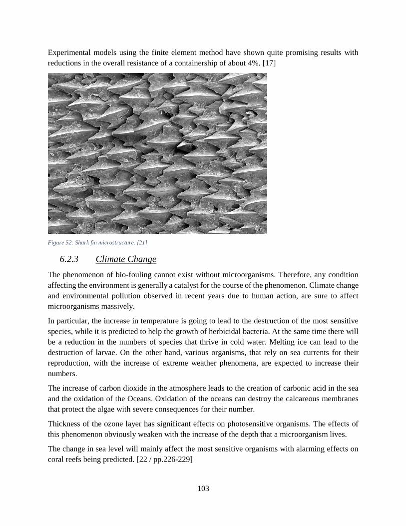
103

Experimental models using the finite element method have shown quite promising results with

reductions in the overall resistance of a containership of about 4%. [17]

Figure 52: Shark fin microstructure. [21]

6.2.3 Climate Change

The phenomenon of bio-fouling cannot exist without microorganisms. Therefore, any condition

affecting the environment is generally a catalyst for the course of the phenomenon. Climate change

and environmental pollution observed in recent years due to human action, are sure to affect

microorganisms massively.

In particular, the increase in temperature is going to lead to the destruction of the most sensitive

species, while it is predicted to help the growth of herbicidal bacteria. At the same time there will

be a reduction in the numbers of species that thrive in cold water. Melting ice can lead to the

destruction of larvae. On the other hand, various organisms, that rely on sea currents for their

reproduction, with the increase of extreme weather phenomena, are expected to increase their

numbers.

The increase of carbon dioxide in the atmosphere leads to the creation of carbonic acid in the sea

and the oxidation of the Oceans. Oxidation of the oceans can destroy the calcareous membranes

that protect the algae with severe consequences for their number.

Thickness of the ozone layer has significant effects on photosensitive organisms. The effects of

this phenomenon obviously weaken with the increase of the depth that a microorganism lives.

The change in sea level will mainly affect the most sensitive organisms with alarming effects on

coral reefs being predicted. [22 / pp.226-229]