Essential Mathematical Methods for Physicists - Weber …williamsgj.people.cofc.edu/Fourier...

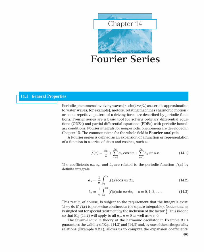
Chapter 14

Fourier Series

14.1 General Properties

Periodic phenomena involving waves [∼ sin(2πx/λ) as a crude approximationto water waves, for example], motors, rotating machines (harmonic motion),or some repetitive pattern of a driving force are described by periodic func-tions. Fourier series are a basic tool for solving ordinary differential equa-tions (ODEs) and partial differential equations (PDEs) with periodic bound-ary conditions. Fourier integrals for nonperiodic phenomena are developed inChapter 15. The common name for the whole field is Fourier analysis.

A Fourier series is defined as an expansion of a function or representationof a function in a series of sines and cosines, such as

f (x) = a0

2+

∞∑n=1

an cos nx +∞∑

n=1

bn sin nx. (14.1)

The coefficients a0, an, and bn are related to the periodic function f (x) bydefinite integrals:

an = 1π

∫ 2π

0f (x) cos nx dx, (14.2)

bn = 1π

∫ 2π

0f (x) sin nx dx, n = 0, 1, 2, . . . . (14.3)

This result, of course, is subject to the requirement that the integrals exist.They do if f (x) is piecewise continuous (or square integrable). Notice that a0

is singled out for special treatment by the inclusion of the factor 12 . This is done

so that Eq. (14.2) will apply to all an, n = 0 as well as n > 0.The Sturm–Liouville theory of the harmonic oscillator in Example 9.1.4

guarantees the validity of Eqs. (14.2) and (14.3) and, by use of the orthogonalityrelations (Example 9.2.1), allows us to compute the expansion coefficients.

663

664 Chapter 14 Fourier Series

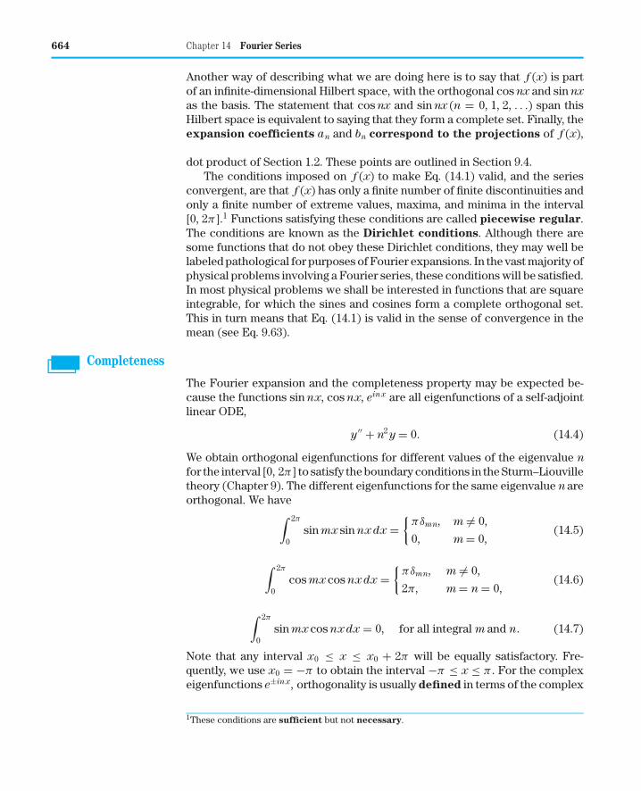
Another way of describing what we are doing here is to say that f (x) is partof an infinite-dimensional Hilbert space, with the orthogonal cos nx and sin nx

as the basis. The statement that cos nx and sin nx (n = 0, 1, 2, . . .) span thisHilbert space is equivalent to saying that they form a complete set. Finally, theexpansion coefficients an and bn correspond to the projections of f (x),with the integral inner products [Eqs. (14.2) and (14.3)] playing the role of thedot product of Section 1.2. These points are outlined in Section 9.4.

The conditions imposed on f (x) to make Eq. (14.1) valid, and the seriesconvergent, are that f (x) has only a finite number of finite discontinuities andonly a finite number of extreme values, maxima, and minima in the interval[0, 2π ].1 Functions satisfying these conditions are called piecewise regular.The conditions are known as the Dirichlet conditions. Although there aresome functions that do not obey these Dirichlet conditions, they may well belabeled pathological for purposes of Fourier expansions. In the vast majority ofphysical problems involving a Fourier series, these conditions will be satisfied.In most physical problems we shall be interested in functions that are squareintegrable, for which the sines and cosines form a complete orthogonal set.This in turn means that Eq. (14.1) is valid in the sense of convergence in themean (see Eq. 9.63).

Completeness

The Fourier expansion and the completeness property may be expected be-cause the functions sin nx, cos nx, einx are all eigenfunctions of a self-adjointlinear ODE,

y′′ + n2 y = 0. (14.4)

We obtain orthogonal eigenfunctions for different values of the eigenvalue n

for the interval [0, 2π ] to satisfy the boundary conditions in the Sturm–Liouvilletheory (Chapter 9). The different eigenfunctions for the same eigenvalue n areorthogonal. We have∫ 2π

0sin mx sin nx dx =

{πδmn, m �= 0,

0, m = 0,(14.5)

∫ 2π

0cos mx cos nx dx =

{πδmn, m �= 0,

2π, m = n = 0,(14.6)

∫ 2π

0sin mx cos nx dx = 0, for all integral m and n. (14.7)

Note that any interval x0 ≤ x ≤ x0 + 2π will be equally satisfactory. Fre-quently, we use x0 = −π to obtain the interval −π ≤ x ≤ π . For the complexeigenfunctions e±inx, orthogonality is usually defined in terms of the complex

1These conditions are sufficient but not necessary.

14.1 General Properties 665

conjugate of one of the two factors,∫ 2π

0(eimx)∗einxdx = 2πδmn. (14.8)

This agrees with the treatment of the spherical harmonics (Section 11.5).

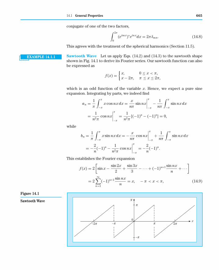
EXAMPLE 14.1.1 Sawtooth Wave Let us apply Eqs. (14.2) and (14.3) to the sawtooth shapeshown in Fig. 14.1 to derive its Fourier series. Our sawtooth function can alsobe expressed as

f (x) ={

x, 0 ≤ x < π,x − 2π, π ≤ x ≤ 2π,

which is an odd function of the variable x. Hence, we expect a pure sineexpansion. Integrating by parts, we indeed find

an = 1π

∫ π

−π

x cos nx dx = x

nπsin nx

∣∣∣∣π

−π

− 1nπ

∫ π

−π

sin nx dx

= 1n2π

cos nx

∣∣∣∣π

−π

= 1n2π

[(−1)n − (−1)n] = 0,

while

bn = 1π

∫ π

−π

x sin nx dx = − x

nπcos nx

∣∣∣∣π

−π

+ 1nπ

∫ π

−π

sin nx dx

= −2n

(−1)n − 1n2π

cos nx

∣∣∣∣π

−π

= −2n

(−1)n.

This establishes the Fourier expansion

f (x) = 2[

sin x − sin 2x

2+ sin 3x

3− · · · + (−1)n+1 sin nx

n+ · · ·

]

= 2∞∑

n=1

(−1)n+1 sin nx

n= x, − π < x < π, (14.9)

x

y

p

–2p

–p

2p0

–p p

Figure 14.1

Sawtooth Wave


which converges only conditionally, not absolutely, because of the disconti-nuity of f (x) at x = ±π. It makes no difference whether a discontinuity isin the interior of the expansion interval or at its ends: It will give rise to con-ditional convergence of the Fourier series. In terms of physical applicationswith x = ω a frequency, conditional convergence means that our square waveis dominated by high-frequency components. ■

Behavior of Discontinuities

The behavior at x = nπ is an example of a general rule that at a finite dis-continuity the series converges to the arithmetic mean. For a discontinuity atx = x0 the series yields

f (x0) = 12

[ f (x0 + 0) + f (x0 − 0)], (14.10)

where the arithmetic mean of the right and left approaches to x = x0. A generalproof using partial sums is given by Jeffreys and by Carslaw (see AdditionalReading).

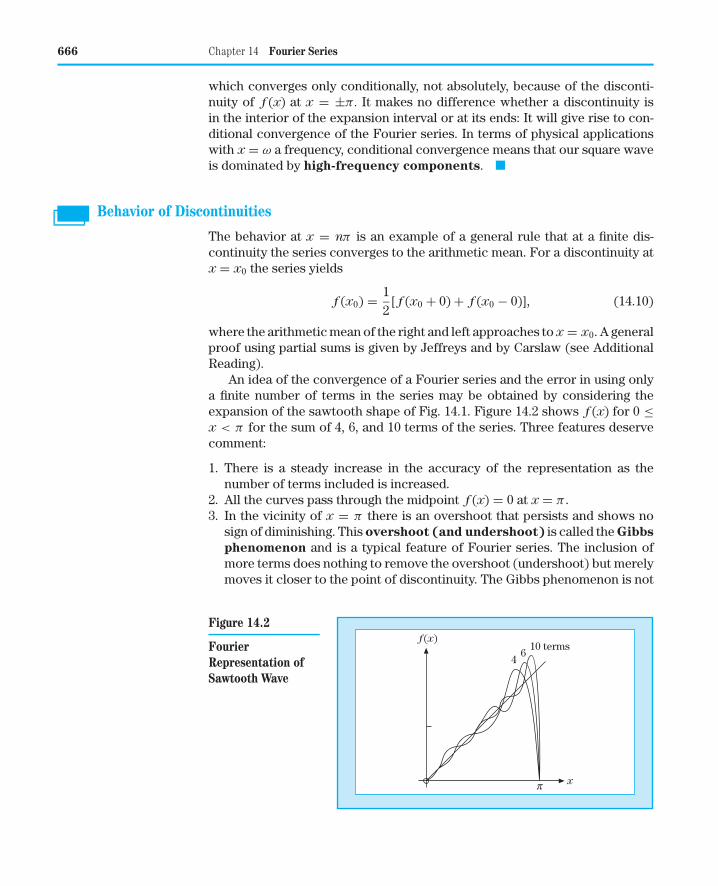
An idea of the convergence of a Fourier series and the error in using onlya finite number of terms in the series may be obtained by considering theexpansion of the sawtooth shape of Fig. 14.1. Figure 14.2 shows f (x) for 0 ≤x < π for the sum of 4, 6, and 10 terms of the series. Three features deservecomment:

1. There is a steady increase in the accuracy of the representation as thenumber of terms included is increased.

2. All the curves pass through the midpoint f (x) = 0 at x = π .3. In the vicinity of x = π there is an overshoot that persists and shows no

sign of diminishing. This overshoot (and undershoot) is called the Gibbs

phenomenon and is a typical feature of Fourier series. The inclusion ofmore terms does nothing to remove the overshoot (undershoot) but merelymoves it closer to the point of discontinuity. The Gibbs phenomenon is not

x

f(x)

46

10 terms

p

Figure 14.2

FourierRepresentation ofSawtooth Wave


f(t)

wtp 2p–2p –p

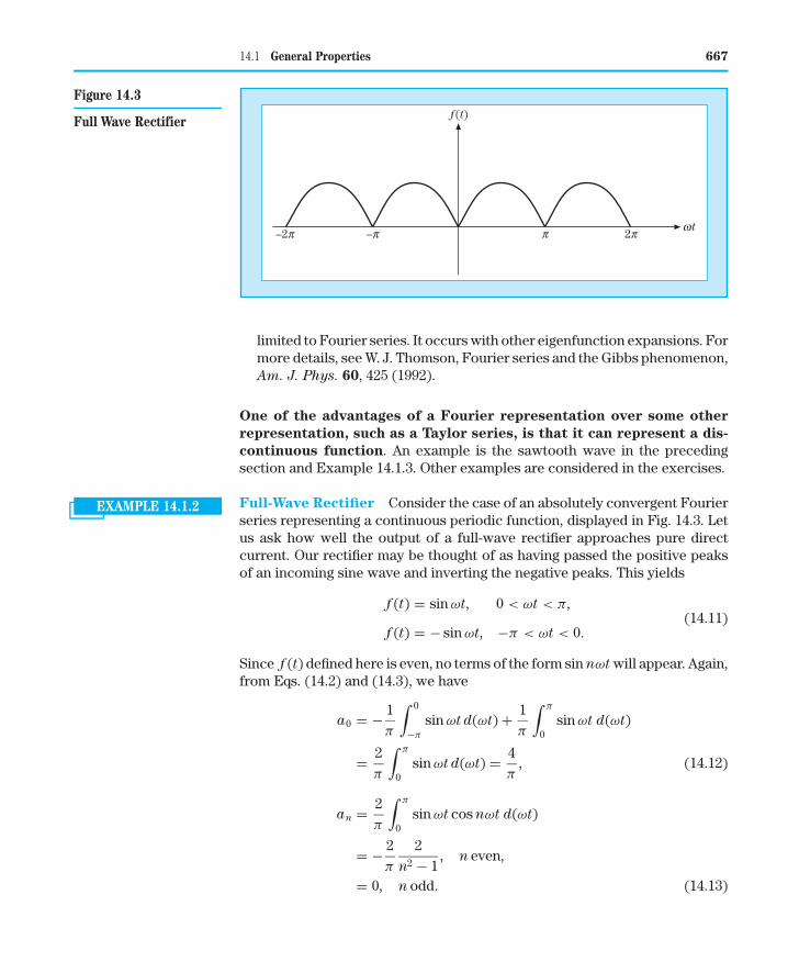
Figure 14.3

Full Wave Rectifier

limited to Fourier series. It occurs with other eigenfunction expansions. Formore details, see W. J. Thomson, Fourier series and the Gibbs phenomenon,Am. J. Phys. 60, 425 (1992).

One of the advantages of a Fourier representation over some other

representation, such as a Taylor series, is that it can represent a dis-

continuous function. An example is the sawtooth wave in the precedingsection and Example 14.1.3. Other examples are considered in the exercises.

EXAMPLE 14.1.2 Full-Wave Rectifier Consider the case of an absolutely convergent Fourierseries representing a continuous periodic function, displayed in Fig. 14.3. Letus ask how well the output of a full-wave rectifier approaches pure directcurrent. Our rectifier may be thought of as having passed the positive peaksof an incoming sine wave and inverting the negative peaks. This yields

f (t) = sin ωt, 0 < ωt < π,(14.11)

f (t) = − sin ωt, −π < ωt < 0.

Since f (t) defined here is even, no terms of the form sin nωt will appear. Again,from Eqs. (14.2) and (14.3), we have

a0 = − 1π

∫ 0

−π

sin ωt d(ωt) + 1π

∫ π

0sin ωt d(ωt)

= 2π

∫ π

0sin ωt d(ωt) = 4

π, (14.12)

an = 2π

∫ π

0sin ωt cos nωt d(ωt)

= − 2π

2n2 − 1

, n even,

= 0, n odd. (14.13)


f(x)

x

h

p 2p 3p–p–2p–3p

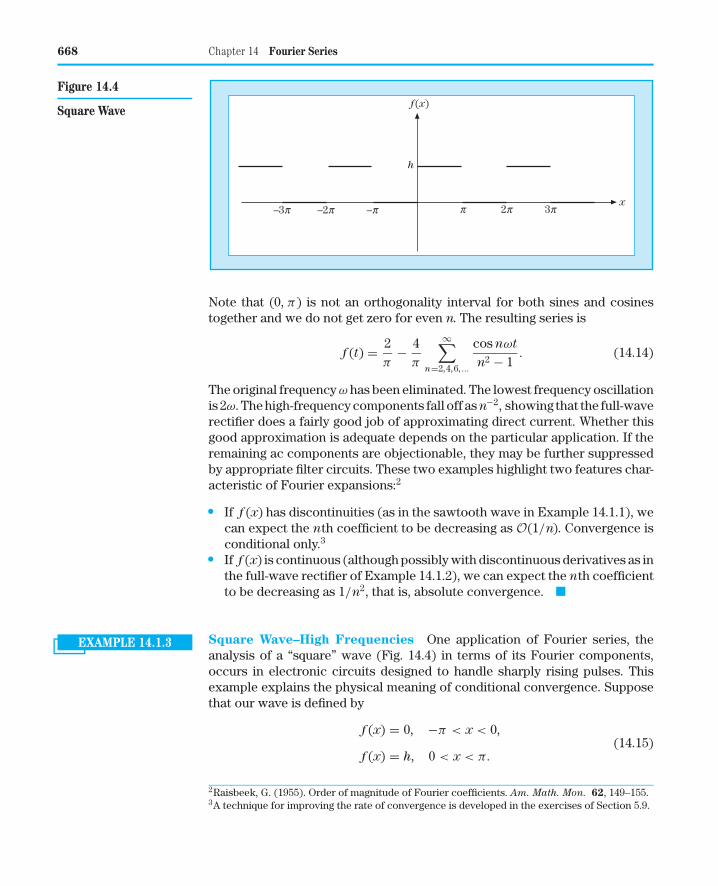
Figure 14.4

Square Wave

Note that (0, π) is not an orthogonality interval for both sines and cosinestogether and we do not get zero for even n. The resulting series is

f (t) = 2π

− 4π

∞∑n=2,4,6,...

cos nωt

n2 − 1. (14.14)

The original frequency ω has been eliminated. The lowest frequency oscillationis 2ω. The high-frequency components fall off as n−2, showing that the full-waverectifier does a fairly good job of approximating direct current. Whether thisgood approximation is adequate depends on the particular application. If theremaining ac components are objectionable, they may be further suppressedby appropriate filter circuits. These two examples highlight two features char-acteristic of Fourier expansions:2

• If f (x) has discontinuities (as in the sawtooth wave in Example 14.1.1), wecan expect the nth coefficient to be decreasing as O(1/n). Convergence isconditional only.3

• If f (x) is continuous (although possibly with discontinuous derivatives as inthe full-wave rectifier of Example 14.1.2), we can expect the nth coefficientto be decreasing as 1/n2, that is, absolute convergence. ■

EXAMPLE 14.1.3 Square Wave–High Frequencies One application of Fourier series, theanalysis of a “square” wave (Fig. 14.4) in terms of its Fourier components,occurs in electronic circuits designed to handle sharply rising pulses. Thisexample explains the physical meaning of conditional convergence. Supposethat our wave is defined by

f (x) = 0, −π < x < 0,(14.15)

f (x) = h, 0 < x < π.

2Raisbeek, G. (1955). Order of magnitude of Fourier coefficients. Am. Math. Mon. 62, 149–155.3A technique for improving the rate of convergence is developed in the exercises of Section 5.9.


From Eqs. (14.2) and (14.3) we find

a0 = 1π

∫ π

0h dt = h, (14.16)

an = 1π

∫ π

0h cos nt dt = 0, n = 1, 2, 3, . . . , (14.17)

bn = 1π

∫ π

0h sin nt dt = h

nπ(1 − cos nπ); (14.18)

bn = 2h

nπ, n odd, (14.19)

bn = 0, n even. (14.20)

The resulting series is

f (x) = h

2+ 2h

π

(sin x

1+ sin 3x

3+ sin 5x

5+ · · ·

). (14.21)

Except for the first term, which represents an average of f (x) over the in-terval [−π, π ], all the cosine terms have vanished. Since f (x) − h/2 is odd,we have a Fourier sine series. Although only the odd terms in the sine seriesoccur, they fall only as n−1. This conditional convergence is like that of theharmonic series. Physically, this means that our square wave contains a lot ofhigh-frequency components. If the electronic apparatus will not pass thesecomponents, our square wave input will emerge more or less rounded off,perhaps as an amorphous blob. ■

Biographical Data

Fourier, Jean Baptiste Joseph, Baron. Fourier, a French mathematician,was born in 1768 in Auxerre, France, and died in Paris in 1830. After his grad-uation from a military school in Paris, he became a professor at the school in1795. In 1808, after his great mathematical discoveries involving the seriesand integrals named after him, he was made a baron by Napoleon. Earlier,he had survived Robespierre and the French Revolution. When Napoleon re-turned to France in 1815 after his abdication and first exile to Elba, Fourierrejoined him and, after Waterloo, fell out of favor for a while. In 1822, hisbook on the Analytic Theory of Heat appeared and inspired Ohm to newthoughts on the flow of electricity.

SUMMARY Fourier series are finite or infinite sums of sines and cosines that describeperiodic functions that can have discontinuities and thus represent a widerclass of functions than we have considered so far. Because sin nx, cos nx areeigenfunctions of a self-adjoint ODE, the classical harmonic oscillator equa-tion, the Hilbert space properties of Fourier series are consequences of theSturm–Liouville theory.


EXERCISES

14.1.1 A function f (x) (quadratically integrable) is to be represented by afinite Fourier series. A convenient measure of the accuracy of theseries is given by the integrated square of the deviation

p =∫ 2π

0

[f (x) − a0

2−

p∑n=1

(an cos nx + bn sin nx)

]2

dx.

Show that the requirement that p be minimized, that is,

∂p

∂an

= 0,∂p

∂bn

= 0,

for all n, leads to choosing an and bn, as given in Eqs. (14.2) and (14.3).Note. Your coefficients an and bn are independent of p. This indepen-dence is a consequence of orthogonality and would not hold for powersof x, fitting a curve with polynomials.

14.1.2 In the analysis of a complex waveform (ocean tides, earthquakes, mu-sical tones, etc.) it might be more convenient to have the Fourier serieswritten as

f (x) = a0

2+

∞∑n=1

αn cos(nx − θn).

Show that this is equivalent to Eq. (14.1) with

an = αn cos θ , α2n = a2

n + b2n,

bn = αn sin θ , tan θn = bn/an.

Note. The coefficients α2n as a function of n define what is called the

power spectrum. The importance of α2n lies in its invariance under a

shift in the phase θn.

14.1.3 Assuming that∫ π

−π[ f (x)]2dx is finite, show that

limm→∞ am = 0, lim

m→∞ bm = 0.

Hint. Integrate [ f (x) − sn(x)]2, where sn(x) is the nth partial sum, anduse Bessel’s inequality (Section 9.4). For our finite interval the assump-tion that f (x) is square integrable (

∫ π

−π| f (x)|2 dx is finite) implies that∫ π

−π| f (x)| dx is also finite. The converse does not hold.

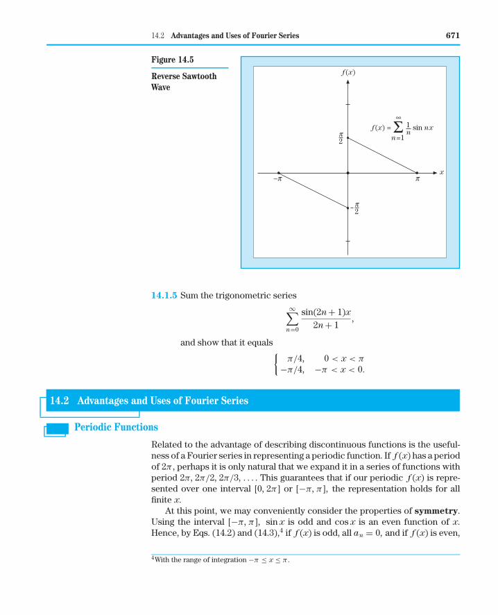
14.1.4 Apply the summation technique of this section to show that

∞∑n=1

sin nx

n=

{ 12 (π − x), 0 < x ≤ π

− 12 (π + x), −π ≤ x < 0

(Fig. 14.5).

14.2 Advantages and Uses of Fourier Series 671

f(x)

px

–p

p2

p2

f(x) = sin nx1n

n=1

∞

Σ

Figure 14.5

Reverse SawtoothWave

14.1.5 Sum the trigonometric series∞∑

n=0

sin(2n + 1)x2n + 1

,

and show that it equals{π/4, 0 < x < π

−π/4, −π < x < 0.

14.2 Advantages and Uses of Fourier Series

Periodic Functions

Related to the advantage of describing discontinuous functions is the useful-ness of a Fourier series in representing a periodic function. If f (x) has a periodof 2π , perhaps it is only natural that we expand it in a series of functions withperiod 2π, 2π/2, 2π/3, . . . . This guarantees that if our periodic f (x) is repre-sented over one interval [0, 2π ] or [−π, π ], the representation holds for allfinite x.

At this point, we may conveniently consider the properties of symmetry.Using the interval [−π, π ], sin x is odd and cos x is an even function of x.Hence, by Eqs. (14.2) and (14.3),4 if f (x) is odd, all an = 0, and if f (x) is even,

4With the range of integration −π ≤ x ≤ π .


all bn = 0. In other words,

f (x) = a0

2+

∞∑n=1

an cos nx, f (x) even, (14.22)

f (x) =∞∑

n=1

bn sin nx, f (x) odd. (14.23)

Frequently, these properties are helpful in expanding a given function.We have noted that the Fourier series is periodic. This is important in

considering whether Eq. (14.1) holds outside the initial interval. Suppose weare given only that

f (x) = x, 0 ≤ x < π (14.24)

and are asked to represent f (x) by a series expansion. Let us take three of theinfinite number of possible expansions:

1. If we assume a Taylor expansion, we have

f (x) = x, (14.25)

a one-term series. This (one-term) series is defined for all finite x.2. Using the Fourier cosine series [Eq. (14.22)], we predict that

f (x) = −x, −π < x≤ 0,

f (x) = 2π − x, π < x≤ 2π.(14.26)

3. Finally, from the Fourier sine series [Eq. (14.23)], we have

f (x) = x, −π < x≤ 0,

f (x) = x − 2π, π < x≤ 2π.(14.27)

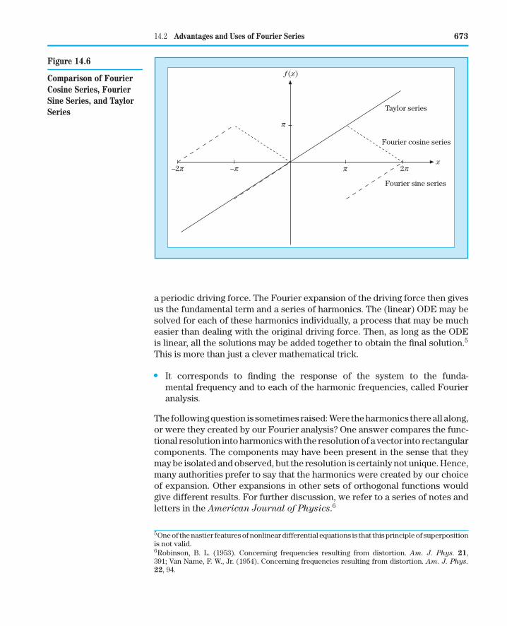
These three possibilities—Taylor series, Fourier cosine series, and Fouriersine series—are each perfectly valid in the original interval [0, π ]. Outside,however, their behavior is strikingly different (compare Fig. 14.6). Whichof the three, then, is correct? This question has no answer, unless we aregiven more information about f (x). It may be any of the three or none ofthem. Our Fourier expansions are valid over the basic interval. Unless thefunction f (x) is known to be periodic, with a period equal to our basic in-terval, or (1/n)th of our basic interval, there is no assurance whatever thatthe representation [Eq. (14.1)] will have any meaning outside the basic inter-val. Clearly, the interval of length 2π, which defines the expansion, makes areal difference for a nonperiodic function because the Fourier series repeatsthe pattern of the basic interval in adjacent intervals. This also follows fromFig. 14.6.

In addition to the advantages of representing discontinuous and periodicfunctions, there is a third very real advantage in using a Fourier series. Supposethat we are solving the equation of motion of an oscillating particle, subject to


f (x)

2px

–p

p

Taylor series

Fourier cosine series

Fourier sine series

p–2p

Figure 14.6

Comparison of FourierCosine Series, FourierSine Series, and TaylorSeries

a periodic driving force. The Fourier expansion of the driving force then givesus the fundamental term and a series of harmonics. The (linear) ODE may besolved for each of these harmonics individually, a process that may be mucheasier than dealing with the original driving force. Then, as long as the ODEis linear, all the solutions may be added together to obtain the final solution.5

This is more than just a clever mathematical trick.

• It corresponds to finding the response of the system to the funda-mental frequency and to each of the harmonic frequencies, called Fourieranalysis.

The following question is sometimes raised: Were the harmonics there all along,or were they created by our Fourier analysis? One answer compares the func-tional resolution into harmonics with the resolution of a vector into rectangularcomponents. The components may have been present in the sense that theymay be isolated and observed, but the resolution is certainly not unique. Hence,many authorities prefer to say that the harmonics were created by our choiceof expansion. Other expansions in other sets of orthogonal functions wouldgive different results. For further discussion, we refer to a series of notes andletters in the American Journal of Physics.6

5One of the nastier features of nonlinear differential equations is that this principle of superpositionis not valid.6Robinson, B. L. (1953). Concerning frequencies resulting from distortion. Am. J. Phys. 21,391; Van Name, F. W., Jr. (1954). Concerning frequencies resulting from distortion. Am. J. Phys.

22, 94.


Change of Interval

So far, attention has been restricted to an interval of length 2π . This restrictionmay easily be relaxed. If f (x) is periodic with a period 2L, we may write

f (x) = a0

2+

∞∑n=1

[an cos

nπx

L+ bn sin

nπx

L

], (14.28)

with

an = 1L

∫ L

−L

f (t) cosnπ t

Ldt, n = 0, 1, 2, 3, . . . , (14.29)

bn = 1L

∫ L

−L

f (t) sinnπ t

Ldt, n = 1, 2, 3, . . . , (14.30)

replacing x in Eq. (14.1) with πx/L and t in Eqs. (14.2) and (14.3) with π t/L.[For convenience, the interval in Eqs. (14.2) and (14.3) is shifted to −π ≤ t ≤π .] The choice of the symmetric interval [−L, L] is not essential. For f (x)periodic with a period of 2L, any interval (x0, x0 + 2L) will do. The choice isa matter of convenience or literally personal preference.

If our function f (−x) = f (x) is even in x, then it has a pure cosine seriesbecause, by substituting t → −t,

∫ 0

−L

f (t) cosnπ t

Ldt =

∫ L

0f (t) cos

nπ t

Ldt,

∫ 0

−L

f (t) sinnπ t

Ldt = −

∫ L

0f (t) sin

nπ t

Ldt

so that all bn = 0 and

an = 2L

∫ L

0f (t) cos

nπ t

Ldt.

Similarly, if f (−x) = − f (x) is odd in x, then f (x) has a pure sine serieswith coefficients

bn = 2L

∫ L

0f (t) sin

nπ t

Ldt.

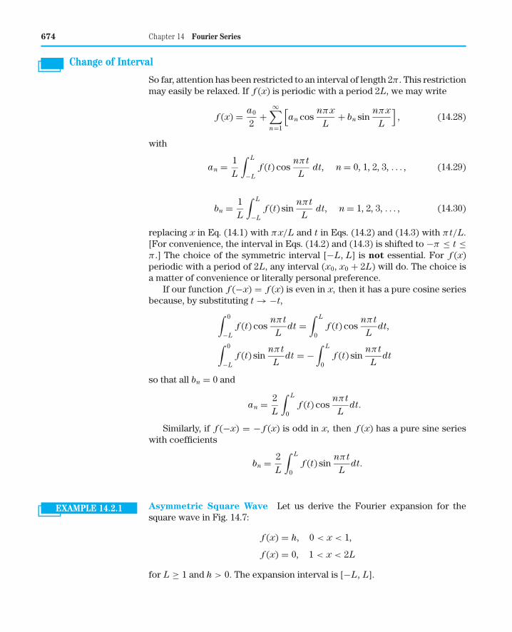
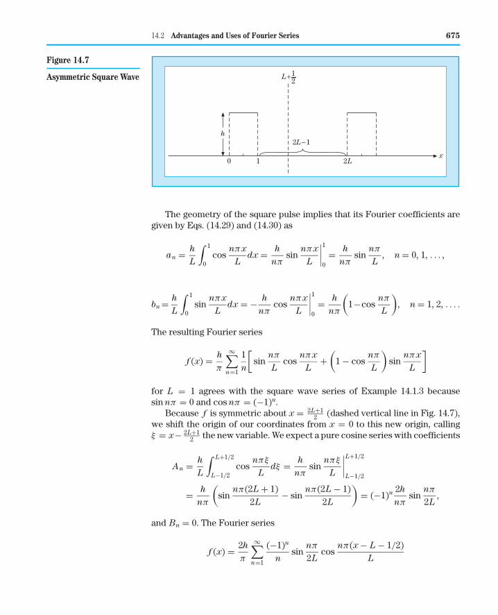
EXAMPLE 14.2.1 Asymmetric Square Wave Let us derive the Fourier expansion for thesquare wave in Fig. 14.7:

f (x) = h, 0 < x < 1,

f (x) = 0, 1 < x < 2L

for L ≥ 1 and h > 0. The expansion interval is [−L, L].


h

2Lx

10

L+21

2L−1

Figure 14.7

Asymmetric Square Wave

The geometry of the square pulse implies that its Fourier coefficients aregiven by Eqs. (14.29) and (14.30) as

an = h

L

∫ 1

0cos

nπx

Ldx = h

nπsin

nπx

L

∣∣∣∣1

0= h

nπsin

nπ

L, n = 0, 1, . . . ,

bn = h

L

∫ 1

0sin

nπx

Ldx = − h

nπcos

nπx

L

∣∣∣∣1

0= h

nπ

(1−cos

nπ

L

), n = 1, 2, . . . .

The resulting Fourier series

f (x) = h

π

∞∑n=1

1n

[sin

nπ

Lcos

nπx

L+

(1 − cos

nπ

L

)sin

nπx

L

]

for L = 1 agrees with the square wave series of Example 14.1.3 becausesin nπ = 0 and cos nπ = (−1)n.

Because f is symmetric about x = 2L+12 (dashed vertical line in Fig. 14.7),

we shift the origin of our coordinates from x = 0 to this new origin, callingξ = x− 2L+1

2 the new variable. We expect a pure cosine series with coefficients

An = h

L

∫ L+1/2

L−1/2cos

nπξ

Ldξ = h

nπsin

nπξ

L

∣∣∣∣L+1/2

L−1/2

= h

nπ

(sin

nπ(2L + 1)2L

− sinnπ(2L − 1)

2L

)= (−1)n 2h

nπsin

nπ

2L,

and Bn = 0. The Fourier series

f (x) = 2h

π

∞∑n=1

(−1)n

nsin

nπ

2Lcos

nπ(x − L − 1/2)L


can be seen to be equivalent to our first result using the addition formulas fortrigonometric functions

cosnπ(x − L − 1/2)

L= (−1)n

[cos

nπ

2Lcos

nπx

L+ sin

nπ

2Lsin

nπx

L

]. ■

EXERCISES

14.2.1 The boundary conditions [such as ψ(0) = ψ(l) = 0] may suggest solu-tions of the form sin(nπx/ l) and eliminate the corresponding cosines.(a) Verify that the boundary conditions used in the Sturm–Liouville

theory are satisfied for the interval (0, l). Note that this is only halfthe usual Fourier interval.

(b) Show that the set of functions ϕn(x) = sin(nπx/ l), n = 1, 2, 3, . . .

satisfies an orthogonality relation∫ l

0ϕm(x)ϕn(x)dx = l

2δmn, n > 0.

14.2.2 (a) Expand f (x) = x in the interval [0, 2L]. Sketch the series you havefound (right-hand side of Answer) over [−2L, 2L].

ANS. x = L − 2L

π

∞∑n=1

1n

sin(

nπx

L

).

(b) Expand f (x) = x as a sine series in the half interval (0, L). Sketchthe series you have found (right-hand side of Answer) over[−2L, 2L].

ANS. x = 4π

∞∑n=0

12n + 1

sin(2n + 1)πx

L.

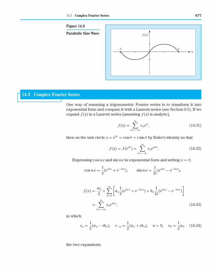
14.2.3 In some problems it is convenient to approximate sin πx over the inter-val [0, 1] by a parabola ax(1 − x), where a is a constant. To get a feelingfor the accuracy of this approximation, expand 4x(1 − x) in a Fouriersine series:

f (x) ={

4x(1 − x), 0 ≤ x ≤ 1

4x(1 + x), −1 ≤ x ≤ 0

}=

∞∑n=1

bn sin nπx.

ANS. bn = 32π3

· 1n3

, n odd

bn = 0, n even

(Fig. 14.8).

14.2.4 Take −π ≤ x ≤ π as the basic interval for the function f (x) = x andrepeat the arguments leading to Eqs. (14.25)–(14.27). Compare yourresults with those in Fig. 14.6 and plot them.

14.3 Complex Fourier Series 677

f (x)

x1–1

Figure 14.8

Parabolic Sine Wave

14.3 Complex Fourier Series

One way of summing a trigonometric Fourier series is to transform it intoexponential form and compare it with a Laurent series (see Section 6.5). If weexpand f (z) in a Laurent series [assuming f (z) is analytic],

f (z) =∞∑

n=−∞cnzn, (14.31)

then on the unit circle z = eiθ = cos θ + i sin θ by Euler’s identity so that

f (z) = f (eiθ ) =∞∑

n=−∞cneinθ . (14.32)

Expressing cos nx and sin nx in exponential form and setting x = θ ,

cos nx = 12

(einx + e−inx), sin nx = 12i

(einx − e−inx),

we may rewrite the general Fourier series [Eq. (14.1)] as

f (x) = a0

2+

∞∑n=1

[an

12

(einx + e−inx) + bn

12i

(einx − e−inx)]

=∞∑

n=−∞cneinx, (14.33)

in which

cn = 12

(an − ibn), c−n = 12

(an + ibn), n > 0, c0 = 12

a0. (14.34)

The Laurent expansion on the unit circle [Eq. (14.32)] has the same form as thecomplex Fourier series [Eq. (14.33)], which shows the equivalence betweenthe two expansions.


When the function f (z) is known, the complex Fourier coefficients may bedirectly derived by projection from it:

cn = 12π

∫ 2π

0e−inx f (x)dx, − ∞ < n < ∞,

based on the orthogonality relation [Eq. (14.8)].

Abel’s Theorem

Consider a function f (z) represented by a convergent power series

f (z) =∞∑

n=0

cnzn =∞∑

n=0

cnrneinθ . (14.35)

This is our Fourier exponential series [Eq. (14.32)]. Separating real and imag-inary parts

u(r, θ) =∞∑

n=0

cnrn cos nθ , v(r, θ) =∞∑

n=1

cnrn sin nθ , (14.36)

the Fourier cosine and sine series. Abel’s theorem asserts that if u(1, θ) andv(1, θ) are convergent for a given θ , then

u(1, θ) + iv(1, θ) = limr→1

f (reiθ ). (14.37)

An application of this theorem appears as Exercise 14.3.11, and it is used inthe next example.

EXAMPLE 14.3.1 Summation of a Complex Fourier Series Consider the series∑∞n=1(1/n) cos nx, x ∈ (0, 2π). Since this series is only conditionally conver-

gent (see Example 5.3.1) and diverges at x = 0 so that Dirichlet’s conditionsare violated, we take

∞∑n=1

cos nx

n= lim

r→1

∞∑n=1

rn cos nx

n(14.38)

absolutely convergent for |r| < 1. Our procedure is again to try forming apower series by transforming the trigonometric functions into exponentialform:

∞∑n=1

rn cos nx

n= 1

2

∞∑n=1

rneinx

n+ 1

2

∞∑n=1

rne−inx

n. (14.39)

Now these power series may be identified as Maclaurin expansions of− ln(1 − z), z = reix, re−ix [Eq. (5.65)], and

∞∑n=1

rn cos nx

n= −1

2[ln(1 − reix) + ln(1 − re−ix)]

= − ln[(1 + r2) − 2r cos x]1/2. (14.40)


Table 14.1Fourier Series Reference

1.∞∑

n=1

1n

sin nx ={

− 12 (π + x), −π ≤ x < 012 (π − x), 0 ≤ x < π

Exercise 14.1.4

Exercise 14.3.3

2.∞∑

n=1

(−1)n+1 1n

sin nx = 12

x, −π < x < πExample 14.1.1

Exercise 14.3.2

3.∞∑

n=0

12n + 1

sin(2n + 1)x ={

−π/4, −π < x < 0

+π/4, 0 < x < π

Exercise 14.1.5

Eq. (14.52)

4.∞∑

n=1

cos nx

n= − ln

[2 sin

( |x|2

)], −π < x < π Eq. (14.38)

5.∞∑

n=1

(−1)n 1n

cos nx = − ln[

2 cos(

x

2

)], −π < x < π Exercise 14.3.11

6.∞∑

n=0

12n + 1

cos(2n + 1)x = 12

ln[

cot|x|2

], −π < x < π (Item 5 – Item 4)

7.∞∑

n=1

(−1)n cos nx

n2 = x2

4− π2

12, −π < x < π Example 14.4.2

8.∞∑

n=0

cos(2n + 1)x(2n + 1)2 = π

4

(π

2− |x|

), −π < x < π Exercise 14.3.4

Letting r = 1 based on Abel’s theorem, we obtain item 4 of Table 14.1∞∑

n=1

cos nx

n= − ln(2 − 2 cos x)1/2

= − ln(

2 sinx

2

), x ∈ (0, 2π).7 (14.41)

Both sides of this expression diverge as x → 0 and 2π . ■

EXERCISES

14.3.1 Develop the Fourier series representation of

f (t) ={

0, −π ≤ ωt ≤ 0,

sin ωt, 0 ≤ ωt ≤ π.

This is the output of a simple half-wave rectifier. It is also an ap-proximation of the solar thermal effect that produces “tides” in theatmosphere.

ANS. f (t) = 1π

+ 12

sin ωt − 2π

∞∑n=2,4,6,...

cos nωt

n2 − 1.

7The limits may be shifted to (−π, π) (and x �= 0) using |x| on the right-hand side.


14.3.2 A sawtooth wave is given by

f (x) = x, −π < x < π.

Show that

f (x) = 2∞∑

n=1

(−1)n+1

nsin nx.

14.3.3 A different sawtooth wave is described by

f (x) ={− 1

2 (π + x), −π ≤ x< 0

+ 12 (π − x), 0 < x≤ π.

Show that f (x) = ∑∞n=1(sin nx/n).

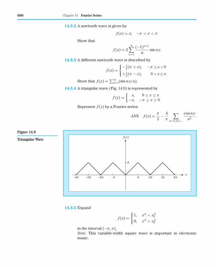
14.3.4 A triangular wave (Fig. 14.9) is represented by

f (x) ={

x, 0 ≤ x ≤ π

−x, −π ≤ x ≤ 0.

Represent f (x) by a Fourier series.

ANS. f (x) = π

2− 4

π

∑n=1,3,5,...

cos nx

n2.

f(x)

xp 2p 3p 4p

p

–p–4p –3p –2p

Figure 14.9

Triangular Wave

14.3.5 Expand

f (x) ={

1, x2 < x20

0, x2 > x20

in the interval [−π, π ].Note. This variable-width square wave is important in electronicmusic.


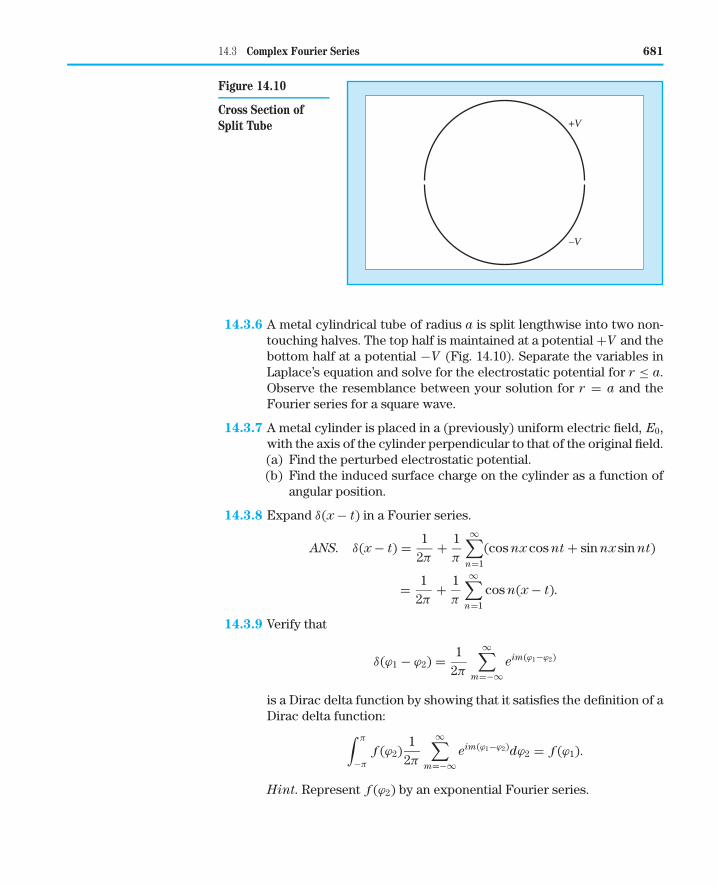
+V

–V

Figure 14.10

Cross Section ofSplit Tube

14.3.6 A metal cylindrical tube of radius a is split lengthwise into two non-touching halves. The top half is maintained at a potential +V and thebottom half at a potential −V (Fig. 14.10). Separate the variables inLaplace’s equation and solve for the electrostatic potential for r ≤ a.Observe the resemblance between your solution for r = a and theFourier series for a square wave.

14.3.7 A metal cylinder is placed in a (previously) uniform electric field, E0,with the axis of the cylinder perpendicular to that of the original field.(a) Find the perturbed electrostatic potential.(b) Find the induced surface charge on the cylinder as a function of

angular position.

14.3.8 Expand δ(x − t) in a Fourier series.

ANS. δ(x − t) = 12π

+ 1π

∞∑n=1

(cos nx cos nt + sin nx sin nt)

= 12π

+ 1π

∞∑n=1

cos n(x − t).

14.3.9 Verify that

δ(ϕ1 − ϕ2) = 12π

∞∑m=−∞

eim(ϕ1−ϕ2)

is a Dirac delta function by showing that it satisfies the definition of aDirac delta function:

∫ π

−π

f (ϕ2)1

2π

∞∑m=−∞

eim(ϕ1−ϕ2)dϕ2 = f (ϕ1).

Hint. Represent f (ϕ2) by an exponential Fourier series.


Note. The continuum analog of this expression is developed in Sec-tion 15.2.

14.3.10 (a) Find the Fourier series representation of

f (x) ={

0, −π < x ≤ 0

x, 0 ≤ x < π.

(b) From the Fourier expansion show that

π2

8= 1 + 1

32+ 1

52+ · · · .

14.3.11 Let f (z) = ln(1 + z) = ∑∞n=1(−1)n+1zn/n. (This series converges to

ln(1 + z) for |z| ≤ 1, except at the point z = −1.)(a) From the imaginary parts (item 5 of Table 14.1) show that

ln(

2 cosθ

2

)=

∞∑n=1

(−1)n+1 cos nθ

n, −π < θ < π.

(b) Using a change of variable, transform part (a) into

− ln(

2 sinθ

2

)=

∞∑n=1

(−1)n+1 cos nθ

n, 0 < θ < 2π.

14.3.12 A symmetric triangular pulse of adjustable height and width is de-scribed by

f (x) ={

a(1 − x/b), 0 ≤ |x| ≤ b

0, b ≤ |x| ≤ π.

(a) Show that the Fourier coefficients are

a0 = ab

π, an = 2ab

π(1 − cos nb)/(nb)2.

Sum the finite Fourier series through n = 10 and through n = 100for x/π = 0(l/9)1. Take a = 1 and b = π/2.

(b) Call a Fourier analysis subroutine (if available) to calculate theFourier coefficients of f (x), a0 through a10.

14.3.13 (a) Using a Fourier analysis subroutine, calculate the Fourier cosinecoefficients a0 through a10 of

f (x) = [1 − (x/π)2]1/2, x ∈ [−π, π ].

(b) Spot check by calculating some of the preceding coefficients bydirect numerical quadrature.

Check values. a0 = 0.785, a2 = 0.284.

14.3.14 A function f (x) is expanded in an exponential Fourier series

f (x) =∞∑

n=−∞cneinx.

14.4 Properties of Fourier Series 683

If f (x) is real, f (x) = f ∗(x), what restriction is imposed on the coef-ficients cn?

14.4 Properties of Fourier Series

Convergence

Note that our Fourier series should not be expected to be uniformly convergentif it represents a discontinuous function. A uniformly convergent series ofcontinuous functions (sin nx, cos nx) always yields a continuous function f (x)(compare Section 5.5). If, however, (i) f (x) is continuous, −π ≤ x ≤ π,(ii) f (−π) = f (+π), and (iii) f ′(x) is sectionally continuous, the Fourierseries for f (x) will converge uniformly. These restrictions do not demandthat f (x) be periodic, but they will be satisfied by continuous, differentiable,periodic functions (period of 2π). For a proof of uniform convergence we referto the literature.8 With or without a discontinuity in f (x), the Fourier serieswill yield convergence in the mean (Section 9.4).

If a function is square integrable, then Sturm–Liouville theory implies thevalidity of the Bessel inequality [Eq. (9.73)]

2a20 +

∞∑n=1

(a2

n + b2n

) ≤ 1π

∫ π

−π

f 2(x)dx (14.42)

so that at least the sum of squares of its Fourier coefficients converges.

EXAMPLE 14.4.1 Absolutely Convergent Fourier Series If the periodic function f (x) has abounded second derivative f ′′(x), then its Fourier series converges absolutely.Note that the converse is not valid, as the full-wave rectifier (Example 14.1.2)demonstrates.

To show this, let us integrate by parts the Fourier coefficients

an = 1π

∫ π

−π

f (x) cos nx dx = f (x) sin nx

nπ

∣∣∣∣∣π

−π

− 1nπ

∫ π

−π

f ′(x) sin nx dx,

where the integrated term vanishes. Because the first derivative f ′(x) is boun-ded a fortiori, |an| = O( 1

n), and similarly bn → 0 for n → ∞, at least as fast

as 1/n, which is not sufficient for absolute convergence. However, anotherintegration by parts can be done, yielding

an = f ′(x) cos nx

n2π

∣∣∣∣∣π

−π

− 1n2π

∫ π

−π

f ′′(x) cos nx dx, (14.43)

8See, for instance, Churchill, R. V. (1993). Fourier Series and Boundary Value Problems, 5th ed.,Section 38. McGraw-Hill, New York.


where the integrated terms cancel each other because f ′ is continuous andperiodic; that is, f ′(π) = f ′(−π). Since | f ′′(x)| ≤ M, we find the upper bound

|an| ≤ M

n2π

∫ π

−π

dx = 2M

n2, (14.44)

which implies absolute convergence (by the integral test of Chapter 5), andthe same applies to bn. ■

If the |an|, |bn| ≤ n−α with 0 < α ≤ 1, then we have at least conditionalconvergence, and the function f (x) may have discontinuities. If α > 1, thenthere is absolute convergence by the integral test of Chapter 5.

Integration

Term-by-term integration of the series

f (x) = a0

2+

∞∑n=1

an cos nx +∞∑

n=1

bn sin nx (14.45)

yields

∫ x

x0

f (x)dx = a0x

2

∣∣∣∣∣x

x0

+∞∑

n=1

an

nsin nx

∣∣∣∣∣x

x0

−∞∑

n=1

bn

ncos nx

∣∣∣∣∣x

x0

. (14.46)

Clearly, the effect of integration is to place an additional power of n in thedenominator of each coefficient. This results in more rapid convergence thanbefore. Consequently, a convergent Fourier series may always be integratedterm by term, with the resulting series converging uniformly to the integral ofthe original function. Indeed, term-by-term integration may be valid even if theoriginal series [Eq. (14.45)] is not convergent. The function f (x) need only beintegrable. A discussion will be found in Jeffreys and Jeffreys, Section 14.06(see Additional Reading).

Strictly speaking, Eq. (14.46) may not be a Fourier series; that is, if a0 �= 0,there will be a term 1

2 a0x. However,∫ x

x0

f (x)dx − 12

a0x (14.47)

will still be a Fourier series.

EXAMPLE 14.4.2 Integration of Fourier Series Consider the sawtooth series for

f (x) = x, −π < x < π. (14.48)

Comparing with Exercise 14.1.1, the Fourier series is

x = 2∞∑

n=1

(−1)n+1 sin nx

n, −π < x < π,


which converges conditionally, but not absolutely, because the harmonic seriesdiverges. Now we integrate it and obtain item 7 of Table 14.1

2∫ x

0

∞∑n=1

(−1)n−1 sin nx

ndx = 2

∞∑n=1

(−1)n−1

n

∫ x

0sin nx dx

= 2∞∑

n=1

(−1)n−1

n2(1 − cos nx)

= π2

6+ 2

∞∑n=1

(−1)n cos nx

n2= x2

2

using Exercise 14.4.1. Because | cos nx| ≤ 1 is bounded and the series∑

n 1/n2

converges, our integrated Fourier series converges absolutely to the limit∫ x

0 x dx = x2/2. ■

Differentiation

The situation regarding differentiation is quite different from that of integra-tion. Here the word is caution.

EXAMPLE 14.4.3 Differentiation of Fourier Series Consider again the series of Exam-ple 14.4.2. Differentiating term by term, we obtain

1 = 2∞∑

n=1

(−1)n+1 cos nx, (14.49)

which is not convergent for any value of x. Warning: Check the convergenceof your derivative.

For a triangular wave (Exercise 14.3.4), in which the convergence is morerapid (and uniform),

f (x) = π

2− 4

π

∞∑n=1,odd

cos nx

n2. (14.50)

Differentiating term by term,

f ′(x) = 4π

∞∑n=1,odd

sin nx

n, (14.51)

which is the Fourier expansion of a square wave

f ′(x) ={

1, 0 < x< π,

−1, −π< x< 0.(14.52)

Inspection of Fig. 14.4 verifies that this is indeed the derivative of our trian-gular wave. ■


• As the inverse of integration, the operation of differentiation has placedan additional factor n in the numerator of each term. This reduces therate of convergence and may, as in the first case mentioned, render thedifferentiated series divergent.

• In general, term-by-term differentiation is permissible under the same con-ditions listed for uniform convergence in Chapter 5.

From the expansion of x and expansions of other powers of x, numerousother infinite series can be evaluated. A few are included in the subsequentexercises.

EXERCISES

14.4.1 Show that integration of the Fourier expansion of f (x) = x, −π < x <

π , leads to

π2

12=

∞∑n=1

(−1)n+1

n2= 1 − 1

4+ 1

9− 1

16+ · · · .

14.4.2 Parseval’s identity.(a) Assuming that the Fourier expansion of f (x) is uniformly conver-

gent, show that

1π

∫ π

−π

[ f (x)]2 dx = a20

2+

∞∑n=1

(a2

n + b2n

).

This is Parseval’s identity. It is actually a special case of the com-pleteness relation [Eq. (9.73)].

(b) Given

x2 = π2

3+ 4

∞∑n=1

(−1)n cos nx

n2, −π ≤ x ≤ π,

apply Parseval’s identity to obtain ζ(4) in closed form.(c) The condition of uniform convergence is not necessary. Show this

by applying the Parseval identity to the square wave

f (x) ={−1, −π < x < 0

1, 0 < x < π

= 4π

∞∑n=1

sin(2n − 1)x2n − 1

.

14.4.3 Show that integrating the Fourier expansion of the Dirac delta function(Exercise 14.3.8) leads to the Fourier representation of the square wave[Eq. (14.21)], with h = 1.Note. Integrating the constant term (1/2π) leads to a term x/2π . Whatare you going to do with this?


14.4.4 Integrate the Fourier expansion of the unit step function

f (x) ={

0, −π < x < 0

x, 0 ≤ x < π.

Show that your integrated series agrees with Exercise 14.3.12.

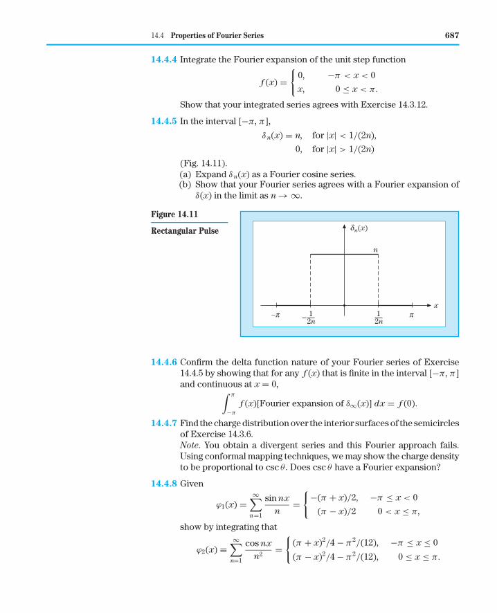
14.4.5 In the interval [−π, π ],

δn(x) = n, for |x| < 1/(2n),

0, for |x| > 1/(2n)

(Fig. 14.11).(a) Expand δn(x) as a Fourier cosine series.(b) Show that your Fourier series agrees with a Fourier expansion of

δ(x) in the limit as n → ∞.

x

12n

–p

dn(x)

n

12n

p

Figure 14.11

Rectangular Pulse

14.4.6 Confirm the delta function nature of your Fourier series of Exercise14.4.5 by showing that for any f (x) that is finite in the interval [−π, π ]and continuous at x = 0,∫ π

−π

f (x)[Fourier expansion of δ∞(x)] dx = f (0).

14.4.7 Find the charge distribution over the interior surfaces of the semicirclesof Exercise 14.3.6.Note. You obtain a divergent series and this Fourier approach fails.Using conformal mapping techniques, we may show the charge densityto be proportional to csc θ . Does csc θ have a Fourier expansion?

14.4.8 Given

ϕ1(x) =∞∑

n=1

sin nx

n=

{−(π + x)/2, −π ≤ x < 0

(π − x)/2 0 < x ≤ π,

show by integrating that

ϕ2(x) ≡∞∑

n=1

cos nx

n2=

{(π + x)2/4 − π2/(12), −π ≤ x ≤ 0

(π − x)2/4 − π2/(12), 0 ≤ x ≤ π.


Additional Reading

Carslaw, H. S. (1921). Introduction to the Theory of Fourier’s Series and

Integrals, 2nd ed. Macmillan, London. Paperback, 3rd ed., Dover, NewYork (1952). This is a detailed and classic work.

Hamming, R. W. (1973). Numerical Methods for Scientists and Engineers, 2nded. McGraw-Hill, New York. Reprinted, Dover, New York (1987).

Jeffreys, H., and Jeffreys, B. S. (1972). Methods of Mathematical Physics, 3rded. Cambridge Univ. Press, Cambridge, UK.

Kufner, A., and Kadlec, J. (1971). Fourier Series. Iliffe, London. This book is aclear account of Fourier series in the context of Hilbert space.

Lanczos, C. (1956). Applied Analysis. Prentice-Hall, Englewood Cliffs, NJ.Reprinted, Dover, New York (1988). The book gives a well-written presen-tation of the Lanczos convergence technique (which suppresses the Gibbsphenomenon oscillations). This and several other topics are presentedfrom the point of view of a mathematician who wants useful numericalresults and not just abstract existence theorems.

Oberhettinger, F. (1973). Fourier Expansions, A Collection of Formulas. Aca-demic Press, New York.

Zygmund, A. (1988). Trigonometric Series. Cambridge Univ. Press, Cambridge,UK. The volume contains an extremely complete exposition, includingrelatively recent results in the realm of pure mathematics.

Essential Mathematical Methods for Physicists - Weber …williamsgj.people.cofc.edu/Fourier...

Documents

Transcript of Essential Mathematical Methods for Physicists - Weber …williamsgj.people.cofc.edu/Fourier...