Entropy and the value of information for investors∗

Antonio Cabrales† Olivier Gossner‡ Roberto Serrano§

May 2011

Abstract: Consider any investor who fears ruin when facing any set of investmentsthat satisfy no-arbitrage. Before investing, he can purchase information about thestate of nature in the form of an information structure. Given his prior, informationstructure α is more informative than information structure β if, whenever he iswilling to buy β at some price, he is also willing to buy α at that price. We showthat this informativeness ordering is complete and is represented by the decreasein entropy of his beliefs, regardless of his preferences, initial wealth, or investmentproblem. We also show that no prior-independent informativeness ordering basedon similar premises exists.

JEL classification numbers: C00, C43, D00, D80, D81, G00, G11.

Keywords: informativeness, information structures, entropy, decision under uncer-

tainty, investment, Blackwell ordering.

∗We thank Bob Aumann, Mark Dean, Itay Fainmesser, Juanjo Ganuza, Johannes Gierlinger,Ehud Lehrer, Jose Penalva, Nicola Persico, Debraj Ray, Larry Samuelson, and David Wolpert foruseful comments.

†Department of Economics, Universidad Carlos III de Madrid‡Paris School of Economics and Department of Mathematics, London School of Economics§Department of Economics, Brown University and IMDEA-Social Sciences Institute

1

1 Introduction

Consider a decision maker operating under uncertainty. When can one say that a

new piece of information is more valuable to this agent than another? This question

is in general hard to answer, because the ranking of information value typically

depends upon at least three considerations. (i) The agent’s priors matter. (An

agent who is almost convinced that a serious crisis in the strength of the dollar is

forthcoming may rank the appearance of bad financial news in China or in Europe

very differently than an agent who is less convinced about such a crisis.) (ii) The

preferences and wealth of the agent matter. (For the same prior, two agents with

different degrees of risk aversion may rank in distinct ways a piece of news that almost

eliminates uncertainty about an unlikely financial loss versus a less precise piece of

news about more likely events.) (iii) The decision problem to which information is

applied matters. (The value of being informed about the likelihood of different risks

depends on the availability of insurance markets for these risks.)

The agent possesses some initial prior on a set of payoff-relevant states of na-

ture. An information structure specifies, for every state of nature, a probability

distribution over the agent’s set of signals, so that each signal leads to an update

of the agent’s beliefs on the state of nature. The question we address is when one

information structure provides more information than another.

The first answer to this fundamental question is provided in the seminal work

of Blackwell (1953). According to Blackwell’s ordering, an information structure is

more informative than another whenever the latter is a garbling of the former, i.e.,

when there exists a stochastic matrix –interpreted as noise– such that the matrix of

conditional probabilities of each signal for the less informative structure is obtained

by multiplying the matrix for the more informative structure by the stochastic ma-

trix. Blackwell’s Theorem states that this is the case if and only if a decision maker

2

with any utility function would prefer to use the former information structure over

the latter when facing any decision problem. This important result provides a

decision-theoretic foundation for Blackwell’s informativeness ordering. Of course,

the requirement that any decision maker would prefer one information structure to

another is very strong, and most pairs of information structures cannot be com-

pared according to Blackwell’s ordering. In other words, Blackwell’s ordering is very

incomplete.

Following recent developments in the theory of riskiness, we attempt here to

formulate an approach based on decision-theoretic principles in order to complete

Blackwell’s ordering.1 Restricting our attention to a class of no-arbitrage investment

decisions first studied in Arrow (1971a) and to a specific class of utility functions that

like to avoid bankruptcy, we postulate the following informativeness ordering. Fixing

a prior over the states, we say that one information structure is more informative

than another if, over the allowed class of problems and preferences, whenever the

first one is rejected at some price, so is the second. This seems a plausible minimum

desideratum for a notion of informativeness.

Our main result is that this informativeness ordering is complete and is repre-

sented by the decrease in entropy of the agent’s beliefs.2 Specifically, if one considers

the prior and the collection of posteriors generated by the information structure, we

show that the informativeness of the information structure is represented by the

difference between the entropy of the prior distribution and the expected entropy

of the conditional posterior distributions.3 More precisely, an information structure

uniformly investment dominates another one in our sense if and only if the entropy

1In particular, we follow closely a recent paper by Hart (2010), in which two orderings areproposed to justify the Aumann and Serrano (2008) index of riskiness and the Foster and Hart(2009) measure of riskiness.

2Unlike the riskiness papers mentioned in the previous footnote, our decision-theoretic consid-erations here do not uncover a new index, but provide a new support to the classic concept ofentropy.

3This difference is referred to as “rate of transmission” by Arrow (1971a), who works with a setof Arrow securities and a logarithmic utility function.

3

decrease resulting from the first is larger than that resulting from the second. Our

ordering is complete, since informativeness is characterized by a real number. It

is also compatible with Blackwell’s ordering, since more information according to

Blackwell’s ordering necessarily corresponds to decrease in entropy.

Our ordering is obtained by restricting our scope to specific classes of prob-

lems and preferences and by basing our approach on total rejection of information

structures. The characterization of this ordering indicates that entropy is the only

objective way to speak of the informativeness of information structures. By con-

struction, our ordering is independent both of the agent’s preferences and of the set

of available choices. On the other hand, it is prior-dependent, which may seem to be

a limitation. We show, however, that this is unavoidable, since any ordering based

on the same postulate as ours is necessarily prior-dependent.4 Therefore, in regard

to the difficulties described in the first paragraph, we provide an environment in

which our complete informativeness ordering takes care of considerations (ii) and

(iii), although it cannot possibly do the same with (i).

Section 2 introduces the investment problems that we study, the basic assump-

tions about the investor, and the notions of an information structure and of valuable

information. Section 3 introduces ruin-averse utility functions, no-arbitrage invest-

ment sets, and our informativeness ordering, and then proves the main result. Sec-

tion 4 offers several points of discussion concerning prior independence and wealth

uniformity, presents an axiomatization of our assumptions on preferences and in-

vestment sets, and analyzes several examples. Section 5 is a review of the literature,

and Section 6 concludes. The Appendix provides the proofs.

4There are of course other limitations, e.g., our postulate of an objective prior.

4

2 Investments and Uncertainty

We measure the value of information according to its relevance to investment choices.

To this end, we rely on a standard model of investment under uncertainty a la Arrow

(1971a).5

2.1 The Investor

We consider an agent with initial wealth w, and with an increasing and twice dif-

ferentiable monetary utility function u : R+ → R. The coefficient of relative risk

aversion at wealth z > 0 is:

ρ(z) = −u′′(z)z

u′(z).

We assume that the agent has weakly increasing relative risk aversion (IRRA),

namely, that ρ is nondecreasing on R+. This standard assumption is defended from

the theoretical point of view by Arrow (1971b). It is also consistent with observed

behavior both in the field (Binswanger, 1981; Post, Assem, van den, Baltussen, and

Thaler, 2008) and in laboratory experiments (Holt and Laury, 2002). The class

of IRRA utility functions includes the widely used constant absolute risk aversion

(CARA) and constant relative risk aversion (CRRA) classes.

We denote by U0 the set of such monetary utility functions. For u ∈ U0, we let

u(0) = limz→0 u(z) ∈ R ∪ {−∞}.

Let K be the finite set of states of nature. The investor has a prior belief p with

full support, fixed throughout the paper.6 An investment opportunity or asset is

b ∈ RK , with the interpretation that if b is taken, the agent’s wealth, once uncertainty

is realized, is w + bk in state k. We do not allow for bankruptcy (the possibility of

negative wealth), and say that an asset b is feasible at wealth w when w+ bk ≥ 0 in

every state k ∈ K.

5This basic asset-investment model is used often, e.g., in Mas-Colell, Whinston, and Green(1995), Section 19.E, where it is integrated into a general-equilibrium economy.

6Except for Subsection 4.1, where we discuss the impossibility of a prior-independent ordering.

5

2.2 The Investments

The investor has the opportunity to choose from an investment set B of assets,

from which he must take one. One possibility among the available choices is to opt

out, namely, to keep his wealth w in a safe asset. We formulate this assumption as

0K ∈ B, where 0K is the null vector of RK . Thus, an investment set consists of a

subset of RK containing 0K . For instance, the set B can consist of a set of Arrow

securities, or of the asset structure of a complete or incomplete market. Elements

in B can be either divisible (for every b ∈ B, λ ∈ [0, 1], λb ∈ B) or indivisible. We

say that an investment set B is feasible at w when all its elements are feasible at w.

2.3 Information Structures

An information structure α is given by a finite set of signals Sα, together with

transition probabilities αk ∈ ∆(Sα) for every k. When the state of nature is k,

αk(s) is the probability that the signal observed by the agent is s. It is standard

practice to represent any such information structure by a stochastic matrix, with

as many rows as states and as many columns as signals; in the matrix, row k is

the probability distribution (αk(s))s∈Sα. We assume that every signal s has positive

probability under at least one state k. This is without loss of generality, since zero

probability signals can be deleted from the set Sα.

It is useful to think of α in terms of a distribution over posterior probabilities.

Signal s has a total probability pα(s) =∑

k p(k)αk(s), and the agent’s posterior

probability on K given s is qsα, derived using Bayes’ formula:

qsα(k) =p(k)αk(s)

pα(s).

Information structures are ranked according to the partial Blackwell (1953) order-

ing. A most informative information structure, denoted as α, is one that perfectly

reveals the state of nature k; hence, for any s, there exists a unique k such that

6

αk(s) > 0. A least informative information structure is any α with no informational

content: (αk(s))s∈Sαis the same distribution for all k.

2.4 Valuable Information

Given a utility function u, initial wealth w, a feasible investment set B, and a

belief q ∈ ∆(K), the maximal expected utility that can be reached by choosing an

investment opportunity b ∈ B is

v(u, w,B, q) = supb∈B, b feasible

∑

k

q(k)u(w + bk)

with the convention that 0 · (−∞) = 0.

The ex-ante expected payoff before receiving signal s from α is

π(α, u, w,B) =∑

s

pα(s)v(u, w,B, qsα).

The possibility of opting out ensures that both v(u, w,B, q) and π(α, u, w,B) are

always larger than or equal to u(w).

The gain V (α, u, w,B) from investment opportunities in B and information α is

the difference:

V (α, u, w,B) = π(α, u, w,B)− u(w).

It is often useful for our purposes to rewrite the above expression in this way:

V (α, u, w,B) =∑

s

pα(s)(v(u, w,B, qsα)− u(w)).

This last expression shows that V (α, u, w,B) > 0 if and only if there exists an s

such that v(u, w,B, qsα) > u(w).

3 Entropy as an Ordering of Information for In-

vestment Problems

3.1 Ruin-Averse Utility and No-Arbitrage Investments

We make two assumptions in our basic framework. One concerns the agent’s utility

function u and the other, the set B of available assets. These two assumptions, taken

7

together, ensure that the class of utility functions and investment sets are suitable

to rank informativeness.

We call an asset b ∈ Rk belief-supported (given initial belief p) if

∑

k p(k)bk ≤ 0,

and we let B∗ be the set of all belief-supported assets. An investment set B is

belief-supported if it contains only belief-supported assets (B ⊆ B∗), and we let

B∗ be the class of belief-supported investment sets. The belief-supported assets are

characterized by the property that no weakly risk-averse or risk-neutral agent with

belief p would prefer to select such an asset over opting out. We also refer to them

as no-arbitrage assets, as they are also characterized by the absence of arbitrage

opportunities (see, e.g., Duffie, 1996, theorem 1 on page 4 and the later discussion

in section 1.B. of risk-neutral probabilities). For instance, for an investor with a

uniform prior over three states, the asset with payoffs (−7, 2, 3) offers no arbitrage

opportunities ex-ante, but it may be a reasonable investment after acquiring appro-

priate information, e.g., that the true state of nature is not state 1.

We call a monetary utility u ruin-averse whenever u(0) = −∞. Thus, a ruin-

averse agent is one who prefers to opt out rather than making any investment that

leads to ruin with positive probability. Let U∗ ⊂ U0 be the set of all ruin-averse

utility functions in our domain. The next lemma, following the analysis of Hart

(2010), characterizes ruin aversion by means of coefficients of risk aversion.

Lemma 1 Let u ∈ U0. Then, u ∈ U∗ if and only if for every z > 0 ρ(z) ≥ 1.

3.2 Information Purchasing

In order to understand the value of information for the agent, we consider a situ-

ation in which the agent has the possibility of purchasing information structure α

before making an investment decision in regard to B. Decisions whether to purchase

information or not are based on the comparison between the expected payoff under

the new information and the sure payoff u(w). The agent with utility function u

8

and wealth w purchases information α at price µ < w, given an investment set B,

when:

π(α, u, w − µ,B) ≥ u(w).

Otherwise, the agent rejects information α at price µ.

Our information ordering is defined as follows:

Definition 1 Information structure α uniformly investment-dominates (or investment-

dominates, for short) information structure β whenever, for every wealth w and price

µ < w such that α is rejected by all agents with utility u ∈ U∗ at wealth w for every

opportunity set B ∈ B∗, β is also rejected by all those agents.

The preceding definition seems plausible as a minimum desideratum in order to

speak of informativeness. The next lemma identifies the important role played in

the definition by an agent with a logarithmic utility function:

Lemma 2 Given an information structure α, a price µ, and a wealth level w > µ, α

is rejected by all agents with utility u ∈ U∗ at wealth level w given every opportunity

set B ∈ B∗ if and only if α is rejected by an agent with ln utility at wealth w for the

opportunity set B∗.

3.3 Entropy Ordering

With the assumptions made about assets and utility functions, our next step is to

arrive at a representation of the ordering just defined. In effect, achieving this repre-

sentation will provide an index of informativeness for information structures, i.e., an

objective way to talk about an information structure being more informative than

another, based on the investment framework described. The result below character-

izes entropy as such an index, which is independent of the specific utility function of

the decision maker, of his wealth, and of the specific investment decision considered.

9

In contrast, such an index cannot be independent of the decision maker’s prior, as

we also show in the next section.

Following Shannon (1948), the entropy of a probability distribution q ∈ ∆(K) is

the quantity:

H(q) = −∑

k∈K

q(k) log2(k),

where 0 log2(0) = 0 by continuity.7 The entropy of p is a measure of the level

of uncertainty about the state of nature held by the investor with belief p. The

entropy is always nonnegative, and is equal to zero only in the case of certainty,

i.e., when q puts weight 1 on some state k. It is concave, representing the fact that

distributions that are closer to the extreme points in ∆(K) correspond to a lower

level of uncertainty. On the other hand, entropy achieves its global maximum at the

uniform distribution, a situation of “maximal uncertainty.”

Recall that following information structure α, (i) the agent’s signal is s with

probability pα(s); and (ii) the posterior probability on K following s is qsα. The

entropy informativeness of information structure α is the expected reduction of

entropy of the investor’s beliefs due to his observation of s. It is this quantity:

I(α) = H(p)−∑

s

pα(s)H(qsα).

As shown in Subsection 4.1, I(α) depends on p as well as on α. (For notational

simplicity, we do not include p as an argument of I. Only in Subsection 4.1 do we

make this dependence explicit.) The informativeness is minimal when α is α with

no informational content, and I(α) = 0. It is maximal when α is α that fully reveals

the state of nature k, and value I(α) = H(p). Note that given a prior p, I is a

numeric index, which hence defines a complete ordering of information structures.

7The specific function log2(·) stems from the normalization that the amount of informationcarried by the observation of a Bernoulli random variable with parameter 1/2 is exactly one bit.For us, any log function would work, including, for example, ln(·).

10

3.4 Main Result

Our main result establishes that the ordering of information structures given by

investment dominance coincides with the ordering according to entropy informa-

tiveness. Hence this ordering is complete.

Theorem 1 Information structure α investment-dominates information structure

β if and only if I(α) ≥ I(β).

4 Discussion

This section discusses each of the assumptions used in our approach.

4.1 Prior-Independent Ordering

For a given prior p, the informativeness ordering we have suggested is represented by

a decrease in entropy. Making the dependence of I(α) on p explicit, we denote here

I(α) by I(α, p). An information structure α is more informative than another β,

I(α, p) ≥ I(β, p), if and only if α causes a larger reduction in entropy (from the

entropy of the prior p to the expected entropy of the generated posteriors) than

does β.

We now prove that there can be no index that orders information structures

that is both compatible with uniform investment dominance and independent of the

agent’s prior. In order to do this, let us define the following.

Definition 2 An information structure α investment-dominates independently of

the prior β, whenever α investment-dominates β for all priors p.

This definition turns out to be too strong a requirement, and leads to the fol-

lowing impossibility result:

Theorem 2 There exists no numerical representation that orders information struc-

tures according to the ordering of investment dominance independently of the prior.

11

4.2 Uniformity in Wealth

After the discussion opened in the previous subsection, we now return to fixing a

prior p, which will remain fixed for the rest of the paper.

We have defined information dominance as wealth-independent, but this is not

really a restriction. To see this, consider the following alternative definition:

Definition 3 Information structure α investment-dominates information structure

β for wealth w if, for every price µ < w such that α is rejected by all agents with

utility u ∈ U∗ for every opportunity set B ∈ B∗, β is also rejected by all those agents.

This definition leads to the following theorem:

Theorem 3 Information structure α investment-dominates information structure

β for wealth w if and only if I(α) ≥ I(β).

The result clearly follows because Lemma 2 holds for either Definition 2 or Def-

inition 3 and the ordering I(·) induced by logarithmic preferences is independent of

wealth.

In a similar vein, we have made so far comparisons for agents with the same

level of wealth. This can be avoided provided the pricing is done as a proportion of

wealth.

Definition 4 Information structure α proportionally investment-dominates infor-

mation structure β if, for any 0 < λ < 1, whenever α is rejected by all agents with

utility u ∈ U∗ for every opportunity set B ∈ B∗ at every wealth w for price λw, β is

also rejected by all those agents.

Before getting to the next result, we prove the following lemma:

Lemma 3 Let 0 < λ < 1. An information structure α is rejected by all agents with

utility u ∈ U∗ for every opportunity set B ∈ B∗ at every wealth w for the price λw

12

if and only if α is rejected by an agent with ln utility at every wealth level for the

opportunity set B∗.

Using Lemma 3 we show:

Theorem 4 Information structure α proportionally investment-dominates infor-

mation structure β if and only if I(α) ≥ I(β).

4.3 On the Ruin-Aversion and No-Arbitrage Assumptions

This subsection is intended to shed additional light on the role of the ruin-averse

utility functions – the class U∗ – and the class of no-arbitrage or belief-supported

investment sets – B∗. So far, the assumptions underlying our main result, theorem 1,

were that (1) the decision makers we study strongly dislike situations in which their

wealth approaches zero (ruin aversion), and (2) the investments they consider do

not offer profitable opportunities in the absence of new additional information (no

arbitrage). Now we offer a joint axiomatization of such economic circumstances, i.e.,

of such preference-investment pairs.

Thus, consider in general any class of utility functions included in our original

IRRA class U0 and any class B of feasible investment sets. First, it is worthwhile

to point out that the classes U∗ of ruin-averse functions and B∗ of no-arbitrage sets

jointly have two properties that we now turn to discuss.

The first property is No Investment under No Information, or NINI for short.

According to this property, in the absence of information beyond the prior p, the

agent prefers to opt out rather than to invest in risky elements of B. As stated,

it is a joint assumption on the possible investment set B and the agent’s utility

function u. It can be viewed as a normalization: for a decision maker who is con-

sidering improving his information before investing, we define his initial position as

“not being ready to invest” if he gets no new information.

13

The NINI property expresses the idea that B is such that V is null unless α has

some informational content; more precisely:

NINI: B is the class of investment sets B such that for

V (α, u, w,B) = 0 for every u ∈ U0, w ∈ R+.

To motivate the second property, we now discuss the circumstances under which

information is valuable to the agent. First, note that if B does not contain feasible

elements b such that bk > 0 in some state k, the agent always weakly prefers to opt

out. More generally, an agent who fully learns that k is the state of nature cannot

take advantage of such information, unless there exists a feasible b offering a gain in

state k. We say that an investment set B is investment-prone if, for every k ∈ K,

there exists b ∈ B such that bk > 0.

What quality of information is needed to ensure that every investor takes advan-

tage of investment-prone sets? We say that information structure α is sometimes

certain if qsα(k) = 1 for some k and s, that is, when there is a signal s which, if

received, reveals that the state of nature is k for sure. If α is not sometimes certain,

we call it always uncertain.

The next lemma shows that sometimes-certain information structures are always

advantageous, provided B is feasible and investment-prone.

Lemma 4 If B is investment-prone and feasible at wealth level w, then V (u, w, α, B) >

0 for every α that is sometimes certain and for every u ∈ U0.

The second joint property of utility functions and investment sets is that only

investors with access to sometimes-certain information structures are always inclined

to invest. This property, (SCAI for short) is expressed as

SCAI: U consists of the elements u of U0 satisfying the condition that there exists a

wealth level w and an investment-prone set B of feasible investment opportu-

nities such that V (α, u, w,B) = 0 for every always-uncertain α.

14

According to SCAI, whenever α is always uncertain, then there exists a feasible

and investment-prone set of investment opportunities such that the agent weakly

prefers to opt out. The idea is that not every piece of information is always valuable,

i.e., valuable for every agent in every circumstance. In particular, risk-averse agents,

like ours, may not use investment opportunities with a positive expected profit if the

associated risk is too high. On the other hand, our agents surely can take advantage

of being fully informed. The SCAI property establishes a restriction on the class

of agents, requiring that only sometimes-certain information structures be always

valuable to them.

As noted above, both the classes U∗ of ruin-averse utility functions and B∗ of

no-arbitrage investment sets satisfy NINI and SCAI. That they satisfy NINI is clear:

no-arbitrage assets offer no profitable investment opportunity to risk-averse agents

if there is no new information. To see that they also satisfy SCAI, think of a typical

investment-prone asset with large negative payoffs in all states but one; with such

no-arbitrage assets around, a risk-averse investor will want to opt out unless the

new information completely reveals one state. Taken together, NINI and SCAI

therefore depict situations in which a risk-averse investor is cautious in utilizing new

information, given that the available investments out there may include very risky

deals.

What is perhaps more surprising is that these two properties uniquely define a

set U of utility functions and a class B of investment sets, and that both U = U∗

and B = B∗:

Theorem 5 U and B satisfy NINI and SCAI if and only if U is the class U∗ of

ruin-averse utility functions, and B is the class B∗ of no-arbitrage investment sets.

15

4.4 Examples

We now compute some examples. The first one illustrates how our framework serves

to complete Blackwell’s ordering.

Example 1 Let K = {1, 2, 3} and fix a uniform prior. Consider two information

structures that are not ordered in the Blackwell sense. For instance, let each of the

two information structures have two signals:

α1 =

1 01 00 1

, α2 =

1 00.1 0.90 1

To see that they are not ranked according to Blackwell, we exhibit two decision

problems where a decision maker would rank them differently. For instance, in Prob-

lem 1 the agent must choose one of two actions: action 1 gives a utility of 1 only in

the first two states, and 0 otherwise, while action 2 gives a utility of 1 only in the

third state, and 0 otherwise. Problem 2, in contrast, has action 1 pay a utility of

1 only in the first state, and 0 otherwise, while action 2 gives a utility of 1 only in

states 2 or 3, and 0 otherwise. Facing Problem 1, the decision maker would value

α1 more than α2: following the first signal in α1, he would choose the first action

and following the second signal in α1, he would choose the second action, thereby

securing a utility of 1. This would be strictly greater than his utility after α2. On

the other hand, facing Problem 2, he would under α2 choose action 1 after the first

signal and action 2 after the second, yielding a utility of 29/30, which is greater than

his optimal utility after α1.

But by calculating their entropy reduction from the uniform prior, we know that

I(α1) > I(α2). Thus, for every investment problem we consider and every utility

function in our allowable class, the first information structure is more valuable –more

informative– than the second when starting from a uniform prior. The difficulty in

the two problems of this example is that, if one specifies an economic environment

16

like ours to make sense of the action-utility pairs provided, the resulting investment

set fails to be belief-supported, for at least some wealth levels.

The second example illustrates the optimization over investment sets.

Example 2 Let the prior belief p and the investment opportunity bi be such that for

a unit of investment the return is:

bik =

{ 1p(k)

− 1 if k = i

−1 if k 6= i.

Then, one can easily see thatK∑

k=1

p(k)bik = 0

and hence, bi is belief-supported given initial belief p. Suppose that B is composed

of a set of K perfectly scalable investment opportunities b1 through bK, one for each

state of nature. Then, suppose wi is the amount an investor invests in bi. This

implies that:

v(ln, w, B, q) = supb∈B, b feasible

K∑

k=1

q(k) ln

(

wk

p (k)

)

so that the optimal w∗k is equal to q(k)w. Hence,

v(ln, w, B, q) =K∑

k=1

q(k) ln

(

q (k)

p (k)

)

+ lnw.

For other CRRA utility functions with parameter φ we can write,

v(φ, w,B, q) = supb∈B, b feasible

K∑

k=1

q(k)

1− φ

(

wk

p (k)

)1−φ

so that the optimal w∗k can be expressed as:

w∗k = λq(k)1/φp (k)−(1−φ)/φ w

with λ = 1/∑K

k=1

(

q(k)1/φp (k)−(1−φ)/φ)

. Hence,

v(φ, w,B, q) =K∑

k=1

q(k)

1− φ

(

q (k)

p (k)λw

)1−φ

φ

.

17

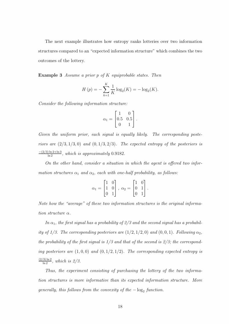
The next example illustrates how entropy ranks lotteries over two information

structures compared to an “expected information structure” which combines the two

outcomes of the lottery.

Example 3 Assume a prior p of K equiprobable states. Then

H (p) = −K∑

k=1

1

Klog2(K) = − log2(K).

Consider the following information structure:

α1 =

1 00.5 0.50 1

.

Given the uniform prior, each signal is equally likely. The corresponding poste-

riors are (2/3, 1/3, 0) and (0, 1/3, 2/3). The expected entropy of the posteriors is

−(2/3) ln 2+ln 3ln 2

, which is approximately 0.9182.

On the other hand, consider a situation in which the agent is offered two infor-

mation structures α1 and α2, each with one-half probability, as follows:

α1 =

1 01 00 1

, α2 =

1 00 10 1

.

Note how the “average” of these two information structures is the original informa-

tion structure α.

In α1, the first signal has a probability of 2/3 and the second signal has a probabil-

ity of 1/3. The corresponding posteriors are (1/2, 1/2, 0) and (0, 0, 1). Following α2,

the probability of the first signal is 1/3 and that of the second is 2/3; the correspond-

ing posteriors are (1, 0, 0) and (0, 1/2, 1/2). The corresponding expected entropy is

(2/3) ln 2ln 2

, which is 2/3.

Thus, the experiment consisting of purchasing the lottery of the two informa-

tion structures is more informative than its expected information structure. More

generally, this follows from the convexity of the − log2 function.

18

Finally, although we have worked with finitely many states to avoid measure-

theoretic technicalities, the results in this paper are easy to extend to distributions

with a continuum of states. This is useful because many applications assume such

a continuum.

Example 4 The normal distribution has a particularly simple entropy. Suppose s

is an n × 1 vector of normally distributed variables, where s ∼ N (µ,Σ) . Then, if

we let |Σ| be the determinant of the variance-covariance matrix, we find that:

H (s) = −1

2log2 ((2πe)

n |Σ|) .

When s follows a univariate uniform distribution in the interval [A,B], then

H(s) can be written as:

H (s) = −

∫ B

A

1

B − Alog2

(

1

B − A

)

du = log2 (B −A) .

It is clear that information structures can be ordered by the expected reduction

on |Σ| in the first case and by the expected reduction of B − A in the second.

5 Related Literature

Other authors have justified the use of the entropy index based on information

theoretic considerations, and have showed that it arises naturally in a variety of

dynamic setups. A salient feature of our work is that it shows that entropy is also

rooted in economic and decision-theoretic arguments in static setups.

Shannon (1948), who introduced entropy as a measure of information, charac-

terizes it as the only measure that jointly satisfies these three properties: continuity,

monotonicity, and decomposability. Marschak (1959) presents formal arguments in

favor of using entropy in the study of the demand for information and its cost. Af-

ter these classic contributions, the concept has arisen separately in several fields of

economics, and we provide only a brief partial survey here.

19

Gossner, Hernandez, and Neyman (2006) study repeated games in which one of

the players, who can forecast the realization of future states of nature, can transmit

information to others through his choice of actions. They provide a closed-form

characterization, based on entropy, of the set of distributions which the players can

achieve.

Gossner and Tomala (2006) analyze games in which a team of players uses pri-

vate signals in a repeated game to secretly coordinate their actions. They show

that entropy is an adequate measure of informativeness to study the trade-off be-

tween the generation of signals for future coordination and the use of acquired secret

information.

The Theil coefficient for economic inequality is based on the entropy of observed

data. Bourguignon (1979) axiomatizes this measure by showing that it is the only

one that is consistent with a property of income-weighted decomposability.

In Sims (2003)’s model of rational inattention, entropy is used to measure in-

formation acquisition by agents with bounded information-processing capabilities.

This approach has been applied to different economic problems. For instance, Peng

(2005) explores its implications for asset-price dynamics and consumption behavior.

Sims (2005) offers a summary of other contributions in this area.

Arrow (1971a) considers an investor who has access to a set of securities that

pay a positive amount in only one state of nature. He shows that, if the value of

information about the state is independent of the returns, then this value is given

by the entropy of this information.

Entropy is also the basis for the relative-entropy measure of proximity of prob-

ability distributions. Blume and Easley (1992) and Sandroni (2000) show that in

dynamic exchange economies, markets favor agents who make the most accurate

predictions when accuracy is measured according to relative entropy. Other appli-

cations of relative entropy include ambiguity aversion (Maccheroni, Marinacci, and

20

Rustichini, 2006) and reputation models (Gossner, 2011).

Measuring the amount of information is a common problem in economics and

decision theory.8 Most of the work in this area follows the seminal work of Black-

well (1953). For Blackwell, an information structure α is more informative than

an information structure β if every decision maker prefers α to β in any decision

problem. As noted in the introduction, the main drawback of this approach is that

this criterion does not provide a complete ordering. Researchers have made progress

by focusing on decision makers who have preferences in a particular class. Lehmann

(1988), for instance, restricts the analysis to problems that generate monotone deci-

sion rules (and hence satisfy single-crossing conditions). Persico (2000), Levin and

Athey (2001), and Jewitt (2007) extend Lehmann’s analysis to more general classes

of monotone problems. We follow this tradition with two main differences. First,

unlike the measures in those papers, our measure of informativeness provides a com-

plete order of all information structures. Second, we achieve this through a different

kind of restriction on admissible preference orderings, and we characterize decision

problems in terms of investment opportunities, thereby restricting the framework.

Gilboa and Lehrer (1991) and Azrieli and Lehrer (2008) take an approach that

differs markedly with respect to the one used in papers cited in the previous para-

graphs. Rather than choosing a class of decision problems, and then providing an

ordering of information structures, they characterize the orderings that are possible

for any prespecified class of decision problems. The 1991 paper considers determin-

istic information structures, and the 2008 paper extends the analysis to stochastic

ones. The entropy function satisfies the axioms of the first paper, and hence it is a

“value of information” function over partitions of the set of states. The 2008 paper

shows that reducibility, weak order, independence, continuity, and convexity char-

acterize all binary relations on information structures induced by decision problems,

8Veldkamp (2011) provides a good summary of ways in which economists have measured infor-mativeness and its applications.

21

entropy being one of them.

A recent paper by Ganuza and Penalva (2010) provides a different way to order

information structures (also a partial order) which is based not on decision-theoretic

considerations, but rather on various measures of dispersion of distributions. (Many

of those measures are presented in Shaked and Shanthikumar, 2007). They show

that while some of their measures are implied by notions of informativeness based on

the value of information, the strongest of their criteria, supermodular precision, is

strictly different: it neither implies nor is implied by those notions of informativeness.

They then proceed to study the implications of greater informativeness (in their

sense) for auction problems, and show that while greater informativeness improves

allocational efficiency, the auction organizers are not always interested in increasing

informativeness since that may increase the buyers’ informational rents.

6 Conclusion

In the classic framework of information structures proposed by Blackwell, we have

found that, for a given prior, a natural informativeness ordering (namely, that if a

decision maker is willing to pay a price for an informative information structure, he

is willing to pay that price for a one that dominates it) is complete when considered

over the class of ruin-averse utility functions and no-arbitrage investment sets. Fur-

thermore, this ordering is represented by the expected decrease of entropy from the

prior to the posteriors, and this ordering is complete. We have also found that no

such ordering can be made independent of the decision maker’s prior.

References

Arrow, K. (1971a): “The value of and demand for information,” in Decision

and Organization, ed. by C. McGuire, and R. Radner, pp. 131–139, Amsterdam.

North-Holland.

22

Arrow, K. J. (1971b): Essays in the Theory of Risk Bearing. Markham Publishing

Company, Chicago.

Aumann, R. J., and R. Serrano (2008): “An economic index of riskiness,”

Journal of Political Economy, 116, 810–836.

Azrieli, Y., and E. Lehrer (2008): “The value of a stochastic information struc-

ture,” Games and Economic Behavior, 63, 679–693.

Binswanger, H. P. (1981): “Attitudes toward risk: Theoretical implications of

an experiment in rural India,” Economic Journal, 91(364), 867–90.

Blackwell, D. (1953): “Equivalent comparison of experiments,” Annals of Math-

ematical Statistics, 24, 265–272.

Blume, L., and D. Easley (1992): “Evolution and market behavior,” Journal of

Economic Theory, 58(1), 9–40.

Bourguignon, F. (1979): “Decomposable income inequality measures,” Econo-

metrica, 47(4), 901–920.

Duffie, D. (1996): Dynamic asset pricing theory. Princeton University Press,

Princeton, N.J.

Foster, D. P., and S. Hart (2009): “An operational measure of riskiness,”

Journal of Political Economy, 117, 785–814.

Ganuza, J.-J., and J. S. Penalva (2010): “Signal orderings based on dispersion

and the supply of private information in auctions,” Econometrica, 78(3), 1007–

1030.

Gilboa, I., and E. Lehrer (1991): “The value of information - an axiomatic

approach,” Journal of Mathematical Economics, 20, 443–459.

23

Gossner, O. (2011): “Simple bounds on the value of a reputation,” Econometrica,

to appear.

Gossner, O., P. Hernandez, and A. Neyman (2006): “Oprimal use of com-

munication resources,” Econometrica, 74(6), 1603–1636.

Gossner, O., and T. Tomala (2006): “Empirical distributions of beliefs under

imperfect observation,” Mathematics of Operations Research, 31(1), 13–30.

Hart, S. (2010): “Comparing risks by acceptance and rejection,” Discussion Pa-

per Series 531, Center for Rationality and Interactive Decision Theory, Hebrew

University of Jerusalem.

Holt, C. A., and S. K. Laury (2002): “Risk aversion and incentive effects,”

American Economic Review, 92(5), 1644–1655.

Jewitt, I. (2007): “Information order in decision and agency problems,” Nuffield

College.

Lehmann, E. L. (1988): “Comparing location experiments,” The Annals of Statis-

tics, 16(2), 521–533.

Levin, J., and S. Athey (2001): “The value of information in monotone deci-

sion problems,” Working Papers 01003, Stanford University, Department of Eco-

nomics.

Maccheroni, F., M. Marinacci, and A. Rustichini (2006): “Ambiguity aver-

sion, robustness, and the variational representation of preferences,” Econometrica,

74(6), 1447–1498.

Marschak, J. (1959): “Remarks on the economics of information,” in Contribu-

tions to Scientific Research in Management, pp. 79–98, Western Data Processing

Center, University of California, Los Angeles.

24

Mas-Colell, A., M. D. Whinston, and J. Green (1995): Microeconomic

Theory. Oxford University Press.

Peng, L. (2005): “Learning with information capacity constraints,” The Journal

of Financial and Quantitative Analysis, 40(2), 307–329.

Persico, N. (2000): “Information acquisition in auctions,” Econometrica, 68(1),

135–148.

Post, T., M. J. Assem, van den, G. Baltussen, and R. H. Thaler (2008):

“Deal or no deal? Decision making under risk in a large-payoff game show,” The

American Economic Review, 98(1), 38–71.

Sandroni, A. (2000): “Do markets favor agents able to make accurate predic-

tions?,” Econometrica, 68, 1303–1341.

Shaked, M., and J. G. Shanthikumar (2007): Stochastic orders. Springer.

Shannon, C. (1948): “A mathematical theory of communication,” Bell System

Technical Journal, 27, 379–423 ; 623–656.

Sims, C. A. (2003): “Implications of rational inattention,” Journal of Monetary

Economics, 50(3), 665–690.

(2005): “Rational inattention: a research agenda,” Discussion paper, Tech-

nical report, Princeton University.

Veldkamp, L. (2011): Information choice in macroeconomics and finance. Prince-

ton University Press, Princeton, NJ.

25

A Proofs

A.1 Proof of Lemma 1

We follow Hart (2010). Assume that for every z > 0,

ρ(z) = −u′′(z)

u′(z)z ≥ 1.

By integrating between z < 1 and 1 we obtain,

ln u′(z)− ln u′(0) ≥ − ln(z),

which can be rewritten as:

u′(z) ≥u′(0)

z.

A second integration between z < 1 and 1 shows that

u(z)− u(1) ≤ u′(0) ln(z),

and hence that u(0) = limz→0 u(z) = −∞.

Now assume that there exists z0 > 0 where ρ(z0) < 1. Since u is IRRA, then for

every z ≤ z0, ρ(z) ≤ ρ(z0) < 1. Integrating shows that for every z ≤ z0,

ln u′(z)− ln u′(z0) ≤ −ρ(z0)(ln(z)− ln(z0)),

which can be expressed as

u′(z) ≤ u′(z0)

(

z

z0

)−ρ(z0)

.

A second integration between z < z0 and z0 shows:

u(z)− u(z0) ≥z0u

′(z0)

1− ρ(z0)

(

(

z

z0

)1−ρ(z0)

− 1

)

.

Since 1 − ρ(z0) > 0, the limits of the right-hand side, and hence of the left-hand

side, are finite. This shows that u(0) > −∞.

26

A.2 Proof of Lemma 2

First, note that the only if condition is satisfied since the ln utility function belongs

to B∗ and B∗ ∈ B∗.

We now prove the if part. Assume that α is rejected at price µ given the

investment set B∗ by an agent with ln utility and with wealth w. For u ∈∗, Lemma

1 shows that ρ(z) ≥ 1 for z > 0; hence:

u′′(z)

u′(z)≤ −

1

z.

By integration between w and z:

{

ln u′(z)− ln u′(w) ≤ − ln(z) + ln(w) if z ≥ w;ln u′(z)− ln u′(w) ≥ − ln(z) + ln(w) if z ≤ w.

Once w is fixed, a second integration with respect to z between w and z′ shows that

for every z′,

u(z′)− u(w) ≤ wu′(w)(ln(z′)− ln(w)).

Hence, given any belief q, B ∈ R∗ and µ < w, we can write:

v(u, w − µ,B, q)− u(w) ≤ wu′(w)(v(ln, w − µ,B, q)− ln(w));

and by summation over qα, for every B ∈∗ and µ < w, we obtain:

π(α, u, w − µ,B)− u(w) ≤ u′(w)w(π(α, ln, w − µ,B)− ln(w)).

Since π(α, u, w−µ,B) is nondecreasing in B, and B∗ is the maximal element of B∗,

then for every B ∈ B∗ and µ < w we have:

π(α, u, w − µ,B)− u(w) ≤ wu′(w)(π(α, ln, w − µ,B∗)− ln(w)) < 0,

which is the desired conclusion.

27

A.3 Proof of Theorem 1

Lemma 2 shows that α uniformly investment-dominates β if and only if, for every

w and µ < w, an agent with ln (or, equivalently, log2) utility function who rejects

α for the opportunity set B∗ also rejects β. The following lemma characterizes the

value of information for an agent with log2 utility function and opportunity set B∗.

Lemma A.1 For every w > 0 and belief q,

1.

v(log2, w, B∗, q) = log2(w)−H(q)−

∑

k

q(k) log2 p(k).

2.

π(α, log2, w, B∗) = I(α) + log2(w).

Proof. For the first point, v(log2, w, B∗, q) is the maximum of

∑

k q(k) log2(w+ bk)

over (bk) such that∑

k p(k)bk ≤ 0. The first-order condition shows that w + bk is

proportional to qkpk, and hence equal to w qk

pk. We then obtain:

v(log2, w, B∗, q) = log2(w) +

∑

k

q(k) log2 q(k)−∑

k

q(k) log2 p(k)

= log2(w)−H(q)−∑

k

q(k) log2 p(k).

For the second point, we rely on the previous expression to deduce:

π(α, log2, w, B∗) =

∑

s

pα(s)v(log2, w, B∗, qα(s))

= log2(w)−∑

s

pα(s)H(qsα)−∑

k,s

pα(s)qsα(k) log2 p(k)

= I(α) + log2(w)

since∑

s pα(s)qsα(k) = p(k).

We now complete the proof of Theorem 1. Recall that by Lemma A.1, an agent

with utility function log2 rejects α at price µ < w for the opportunity set B∗ if and

28

only if:

I(α) < log2

(

w

w − µ

)

.

If I(α) ≥ I(β), then β is rejected whenever α is. If, on the contrary, I(α) < I(β),

let µ be such that:

I(α) < log2

(

w

w − µ

)

< I(β).

At this price µ, α is rejected whereas β is accepted. Hence, α does not investment-

dominate β.

A.4 Proof of Theorem 2

By Theorem 1 and a fixed prior p, the only possible index is I(α, p) = H(p) −

∑

s pα(s)H(qsα). Therefore, it suffices to construct an example to show that this

index orders two information structures in different ways for two different priors.

The example follows.

Let K = {1, 2, 3}. Let p1 = (1/2, 1/2, 0) and p2 = (1/3, 1/3, 1/3) and an agent

with u(x) = ln(x).9

Let information structures α1 and α2 be described by these two-signal three-state

matrices:

α1 =

1 00 10.5 0.5

, α2 =

0.3 0.70 11 0

.

Clearly, the expected utility for the agent with logarithmic utility under α1 is

larger than that for α2 when priors are p1 as the former gives her full information

while the latter does not. It thus follows that:

I(α1, p1) = H(p1)−∑

s

pα1(s)H(qsα1

) > H(p1)−∑

s

pα2(s)H(qsα2

) = I(α2, p1).

What is the expected entropy of the posteriors generated by α1 and α2 under

p2? First, the utility for a ln agent of prior p2 is ln(1/3). Then for α1 the expected

9We make our computations below on the basis of this utility function, but recall that for allx, log2 x = lnx/ ln 2, a positive transformation.

29

utility is:(

2

3

)

ln

(

2

3

)

+

(

1

3

)

ln

(

1

3

)

= −0.63651.

Therefore,

H(p2)−∑

s

pα1(s)H(qsα1

) =(2/3) ln 2

ln 2=

0.462 10

ln 2= 2/3.

As for α2, the (conditional on p2) probability of either signal is 13/30 and 17/30.

After she observes each signal, her posteriors are (3/13, 0, 10/13) and (7/17, 10/17, 0),

respectively. Thus, her expected ln utility from α2 is:

(

13

30

)((

3

13

)

ln

(

3

13

)

+

(

10

13

)

ln

(

10

13

))

+

(

17

30

)((

7

17

)

ln

(

7

17

)

+

(

10

17

)

ln

(

10

17

))

= −0.618 .

Noting that ln(1/3) is the expected utility from the prior, we can derive:

H(p2)−∑

s

pα2(s)H(qsα2

) =0.480 61

ln 2.

That is,

I(α1, p2) = H(p2)−∑

s

pα1(s)H(qsα1

) < H(p2)−∑

s

pα2(s)H(qsα2

) = I(α2, p2).

Hence, whereas for prior p1 information structure α1 is more informative than

α2, the opposite is true for prior p2.

A.5 Proof of Lemma 3 and Theorem 4

For a fixed w, it follows from Lemma 2 that α is rejected by all agents with utility

u ∈ U∗ at wealth w and price λµ if and only if it is rejected by an agent with ln utility

for the opportunity set B∗ at the same wealth level and price. Hence Lemma 3.

Note that the property that an agent with ln utility purchases some information

at price λw for wealth level w is independent of w.

From Lemma 3, α proportionally investment dominates β if and only if, for every

λ, whenever an agent with utility ln and opportunity set B∗ purchases β at some

30

wealth level w for the price λw, the same agent purchases α. This is equivalent to

the fact that given some w > 0 and for every µ, whenever an agent with utility

ln and opportunity set B∗ purchases β at wealth level w for the price µ, the same

agent purchases α. From point 2 of Lemma A.1, this statement is equivalent to

I(α) ≥ I(β). Hence Theorem 4.

A.6 Proof of Lemma 4

Let k, s be such that qsα(k) = 1, and let b ∈ B be such that bk > 0. If bk is feasible,

then we have v(u, w,B, qsα) ≥ u(w + bk) > u(w). Hence,

V (α, u, w,B) ≥ pα(s)(u(w + bk)− u(w)) > 0.

A.7 Proof of Theorem 5

Given a class U ⊆ U0 of utility functions, we say that an investment b individually

satisfies NINI if for every u ∈ U and w ∈ R+ such that b is feasible,

∑

k

p(k)u(w + bk) ≤ u(w).

Thus, b individually satisfies NINI when, under no information, the agent does not

prefer b to opting out. We denote as B the set of investments that individually

satisfy the NINI property. Since 0K satisfies NINI, the NINI investment set is a

nonempty investment set.

Lemma A.2 Given U , B satisfies NINI if and only if B is the class of investment

sets contained in B.

Proof. B satisfies NINI if and only if it contains all the investment sets B such that

for every w > 0 and u ∈ U ,

V (α, u, w,B) = 0.

That is, if B is such that for every w > 0, u ∈ U , it is true that

supb∈B, b feasible

∑

k

p(k)u(w + bk) = 0.

31

An equivalent way to write the previous statement is: for every w > 0, u ∈ U and

b ∈ B feasible, then we have:

∑

k

p(k)u(w + bk) ≤ u(w),

which is finally equivalent to B ⊆ B.

Therefore, we assume from this point on that B is the NINI investment set

corresponding to a set of utility functions U , and that B is the class of investment

sets contained in B.

We say that a set A ⊆ RK is comprehensive if, for every feasible b′ and for every

feasible b ∈ A such that b′k ≤ bk for every k, we also have b′ ∈ A.

Lemma A.3 B is comprehensive.

Proof. Assume that b ∈ B and that b′ is such that b′k ≤ bk for every k. Then, b is

feasible at wealth w whenever b′ is; and for every u ∈ U , w ∈ R+,

∑

k

p(k)u(w + b′k) ≤∑

k

p(k)u(w + bk) ≤ u(w).

Hence, b′ ∈ B.

We observe that if B is not investment-prone, neither is any element of B, a

subset of B. In this case, SCAI becomes trivially equivalent to U = ∅. In contrast,

the following proposition characterizes SCAI when B is investment-prone.

Proposition A.4 If B is investment-prone, then U satisfies SCAI if and only if

U = U∗.

Proof. We divide the proof into a series of lemmata.

Lemma A.5 Let u ∈ U0. If u(0) > −∞, then for every w and for every B that is

investment-prone and feasible, there exists an always-uncertain α such that

V (u, w, α, B) > 0.

32

Proof. Fix u, w, and the set B that is investment-prone and feasible.

For 1 > ε > 0, let αε be defined by Sαε = K, αεk(s) = 1 − ε if k = s, and

αk(s) = εK−1

otherwise. It can easily be werified that αε is always uncertain for

every ε > 0, and that as ε → 0, qkαε(k) → 1 for every s.

Since B is investment-prone, there exist k∗ and b∗ ∈ B such that b∗k∗ > 0. We

now have

v(u, w,B, qk∗

αε) = supb∈B

∑

k

qk∗

αε(k)u(w + bk)

≥∑

k

qk∗

αε(k)u(w + b∗k)

≥ qk∗

αε(k∗)u(w + b∗k∗) + (1− qk∗

αε(k∗))u(0).

Hence,

limε→0

v(u, w,B, qk∗

αε) = u(w + b∗k∗) > u(w),

which shows that for ε small enough, v(u, w,B, qk∗

αε) > 0 and therefore V (u, w, αε, B) >

0.

Lemma A.6 Let u ∈ U0 and assume that B is investment-prone. If u(0) = −∞,

then there exist w and an investment-prone set B that is feasible at w such that

V (u, w, α, B) = 0 for every always-uncertain α.

Proof. Since B is investment-prone, for every k ∈ K there exists b′k such that

b′kk > 0. Let b+ = mink b′kk > 0, and b− = min(mink 6=j b

′kj ,−1) < 0. The investment

bk given by bkk = b+ and bkj = b− for every j 6= k is such that for every j, bkj ≤ b′kj .

Since B is comprehensive from Lemma A.3, it follows that bk ∈ B. Let B be the

investment-prone set B = {0K}∪{bk, k ∈ K}. B is feasible at wealth-level w = −b−.

Let α be always uncertain and assume u(0) = −∞. For every s ∈ Sα and for every

33

bk ∈ B, the expected utility from investing in bk conditional on s is

∑

k′

qsα(k′)u(w + bkk′) = qsα(k)u(w + b+) + (1− qsα(k))u(w + b−)

= qsα(k)u(w + b+) + (1− qsα(k))u(0)

= −∞.

Thus, for every s ∈ Sα,

v(u, w,B, qsα) = u(w),

which implies that:

V (u, w, α, B) = 0.

Lemmata A.5 and A.6 provide the proof of Proposition A.4.

Lemma A.7 If U = U∗, then the only class B that satisfies NINI is the class B∗ of

belief-supported investment sets.

Proof. We need to show that the NINI investment set B coincides with the set B∗

of belief-supported assets.

For any b ∈ B∗, and for any u ∈ U∗ and w such that b is feasible, u is concave

and increasing. This implies:

∑

k

p(k)u(w + bk) ≤ u(w +∑

k

p(k)bk) ≤ u(w),

and hence, b ∈ B.

Now consider b ∈ B. Note that u given by u(z) = ln(z) for z > 0 is in U∗. Hence,

b ∈ B implies that for every w large enough,

∑

k

p(k) ln(w + bk) ≤ ln(w),

which is equivalent to∑

k

p(k) ln(1 +bkw) ≤ 0.

34

Hence, for every ε > 0 small enough,

∑

k

p(k) ln(1 + εbk) ≤ 0.

A first-order Taylor expansion shows that this implies

∑

k

p(k)bk ≤ 0,

and hence, b ∈ B∗.

To wrap up the proof of Theorem 5, assume first that U and B satisfy NINI and

SCAI. Then from Lemma A.2, B is the class of investment sets contained in B. If B

is not investment-prone, then U = ∅, in which case B = RK , a contradiction. Hence,

B is investment-prone, and from Proposition A.4, U = U∗. Finally, it follows from

Lemma A.7 that B = B∗.

We now show that U∗ and B∗ satisfy NINI and SCAI. With the assumption that

B = B∗, U∗ satisfies SCAI from Proposition A.4. With U = U∗, B∗ satisfies NINI

from Lemma A.7.�

35