Energy landscape analysis of the two-dimensional nearest-neighbor φ4 model

Dhagash Mehta∗

Department of Physics, Syracuse University, Syracuse, NY 13244, USA

Michael Kastner†

National Institute for Theoretical Physics (NITheP), Stellenbosch 7600, South Africa andInstitute of Theoretical Physics, University of Stellenbosch, Stellenbosch 7600, South Africa

Jonathan D. Hauenstein‡

Department of Mathematics, Texas A&M University, College Station, TX 77843-3368, USA(Dated: February 15, 2012)

The stationary points of the potential energy function of the φ4 model on a two-dimensionalsquare lattice with nearest-neighbor interactions are studied by means of two numerical methods: anumerical homotopy continuation method and a globally-convergent Newton-Raphson method. Weanalyze the properties of the stationary points, in particular with respect to a number of quantitiesthat have been conjectured to display signatures of the thermodynamic phase transition of the model.Although no such signatures are found for the nearest-neighbor φ4 model, our study illustrates thestrengths and weaknesses of the numerical methods employed.

PACS numbers: 05.50.+q, 64.60.A-, 05.70.Fh

I. INTRODUCTION

The stationary points of the potential energy functionor other classical energy functions can be employed tocalculate or estimate certain physical quantities of inter-est. Well-known examples include transition state theoryor Kramers’s reaction rate theory for the thermally ac-tivated escape from metastable states, where the barrierheight (corresponding to the difference between poten-tial energies at certain stationary points of the potentialenergy function) plays an essential role. More recently,a large variety of related techniques has become popularunder the name of energy landscape methods [1], allow-ing for applications to many-body systems as diverse asmetallic clusters, biomolecules and their folding transi-tions, or glass formers undergoing a glass transition.

In the late 1990s it was observed that properties ofstationary points of the potential energy function V , i. e.configuration space points qs satisfying dV (qs) = 0, re-flect in dynamical and statistical physical quantities si-multaneously and show pronounced signatures near aphase transition [2]. This observation sparked quite someresearch activity, reviewed in [3], including a theorem byFranzosi and Pettini asserting that, at least for a certainclass of models, stationary points with V (qs)/N = vc

are indispensable for the occurrence of an equilibriumphase transition at potential energy vc [4]. This theoremrequires a number of conditions to be satisfied: The po-tential energy function V has to be smooth, confining,and of short-range (see [4] for a complete list of con-ditions and their definitions). At the time when these

∗ dbmehta@syr.edu† kastner@sun.ac.za‡ jhauenst@math.tamu.edu

papers were published, one might have still hoped thatsome of the conditions on V were merely technical, butnot essential for the result. However, it became clearsoon that the result can not be extended to long-rangeinteracting models [5], nor to non-confining potentials [6]:These classes of potentials comprise cases which are par-ticularly amenable to analytic calculations, and a directrelation between phase transitions and stationary pointsof V could be ruled out through exactly solvable coun-terexamples.

Originally, the incentive for the study reported in thepresent article was to investigate the stationary pointsof a model that satisfies all the conditions required byFranzosi and Pettini [4]. This is not an easy task, as inthis class there are no exactly solvable models which havea phase transition [7]. As a model to study, we then optedfor the nearest-neighbor φ4 model on a two-dimensionalsquare lattice. This model, though not exactly solvable,appears to be relatively simple. Moreover, results on thestationary points of its long-range version were knownand readily available for comparison [5].

Much to our surprise, we found that all stationarypoints qs of the potential energy function V have non-positive potential energies, i. e., V (qs) ≤ 0. From thisobservation, one can conclude that the result of Franzosiand Pettini, allegedly proven in [4], is false. Further-more, a numerical method put forward in [8] and appliedto the very same two-dimensional φ4 model yields incor-rect results. These findings, and a discussion of their im-plications, have been published in a Letter [9]. The non-positivity of the stationary energies V (qs) was establishedin that Letter analytically, supported by results obtainedwith two different numerical methods. The main pur-pose of the present article is to give a detailed account ofthese numerical methods and to present a more detailedanalysis of the properties of the stationary points of the

2

two-dimensional nearest-neighbor φ4 model.In Sec. II, this model is introduced and some of its

thermodynamic properties are reviewed. In Sec. III, thefirst of the numerical methods, namely homotopy contin-uation, is discussed. It is an algebraic-geometrical tech-nique devised to obtain all isolated stationary points ofa given system of multivariate polynomial equations, butis restricted to fairly small lattice sizes. We have appliedthis method to square lattices of sizes 3 × 3 and 4 × 4.The stationary points obtained are analyzed with respectto their number, potential energies, indices, and Hessiandeterminants in Sec. IV. The second numerical method,discussed in Sec. V, makes use of a globally convergentversion of the Newton-Raphson algorithm for searchingthe zeros of a real-valued function. It can be applied tolarger lattice sizes, but provides in general only a subsetof the stationary points. We summarize and discuss ourfindings in the concluding Sec. VI.

II. TWO-DIMENSIONAL

NEAREST-NEIGHBOR φ4 MODEL

On a finite square lattice Λ ⊂ Z2 consisting of N = L2

sites, a real degree of freedom φi is assigned to each latticesite i ∈ Λ. By N (i) we denote the subset of Λ consistingof the four nearest-neighboring sites of i on the latticeunder the assumption of periodic boundary conditions.The potential energy function of this model is given by

V (q) =∑

i∈Λ

[

λ

4!q4i −

µ2

2q2i +

J

4

∑

j∈N (i)

(qi − qj)2

]

, (1)

where q = (q1, . . . , qN ) denotes a point in configurationspace Γ = RN [10]. The parameter J > 0 determines thecoupling strength between nearest-neighboring sites andthe parameters λ, µ > 0 characterize a local double-wellpotential each degree of freedom is experiencing.

In the thermodynamic limit N → ∞ this model isknown to undergo, at some critical temperature Tc, acontinuous phase transition, in the sense that the config-urational canonical free energy

f(T ) = − limN→∞

1

Nβln

∫

Γ

dNq e−V (q)/T (2)

is nonanalytic at T = Tc. The transition is from a “ferro-magnetic” phase with nonzero average particle displace-ment to a “paramagnetic” phase with vanishing aver-age displacement (see [11] for more details as well as forMonte Carlo results).

Since we are interested in whether, and how, the phasetransition reflects in the properties of the potential en-ergy landscape, it is more adequate for our purposes tocompare not to Tc, but to the critical potential energyper lattice site, vc, of the transition [12]. Both quantitiesare unambiguously related to each other in the thermo-dynamic limit via the caloric curve v(T ). This is true

independently of the statistical ensemble used, as theseensembles are known to be equivalent for short-rangemodels like the one we are studying [13].

The critical potential energy vc is less frequently stud-ied, in fact the only data we could find in the literatureare from Monte Carlo simulations of fairly small systemsizes N = 20×20 in [14], with parameter values λ = 3/5,µ2 = 2, and J = 1. We use the same values of λ andµ2 in the following, but will show results for a range ofcouplings J . Since the value of vc is a crucial benchmarkwhen relating our stationary point analysis to the phasetransition of the φ4 model, we have performed standardMetropolis Monte Carlo simulations for somewhat largersystem sizes up to 128 × 128 and 107 lattice sweeps.

Some of the Monte Carlo results have already beenreported in [9]. From these plots one can read off a crit-ical potential energy per lattice site of roughly vc ≈ 2.2for coupling J = 1. An improved estimate could be ob-tained by more extensive Monte Carlo simulations and/ora finite-size scaling analysis of the data, but the resultsas they are will be sufficient for our purposes. We havedetermined vc also for a few other couplings, obtainingthe rough estimates vc ≈ −5.0 for J = 0.2 and vc ≈ −3.0for J = 0.35.

III. NUMERICAL POLYNOMIAL HOMOTOPY

CONTINUATION METHOD

The idea behind numerical continuation methods is tofirst find the solutions of a simple system of equationswhich shares several important features with the givensystem. Then, in a second step, starting from these so-lutions one continues them towards the given system ina systematic way. Homotopy continuation methods havebeen around already for several decades [15, 16]. Withmore recent machinery like the numerical polynomial ho-motopy continuation (NPHC) method used in the presentarticle, the method is guaranteed to find all isolated so-lutions of systems of polynomial equations [17, 18].

We consider a system of m polynomial equations

P (q) =

p1(q)...

pm(q)

= 0 (3)

in the variables q = (q1, . . . , qm)T , and we assume that allsolutions of (3) are isolated. Then Bezout’s Theorem (seeChapter 8 of [17]) asserts that a system of m polynomialequations in m variables has at most

∏mi=1 di isolated

solutions where di is the degree of the ith polynomial.This bound is called the classical Bezout bound, and it isknown to be sharp for generic systems [i.e., for genericvalues of the coefficients of the polynomials pi(q)].

The continuation of solutions is formally described bythe homotopy

H(q, t) = P (q)(1 − t) + γtS(q), (4)

3

where γ is a complex number and

S(q) =

s1(q)...

sm(q)

= 0 (5)

is again a system of m polynomial equations. Varyingthe parameter t ∈ [0, 1], H can be deformed from thestart system H(q, 1) = γS(q) at t = 1 into the polynomialsystem of interest, H(q, 0) = P (q) at t = 0. The followingconditions have to be satisfied in order to guarantee thatall solutions of P can be computed from this homotopy:

1. The solutions of S(q) = 0 can be computed.

2. The number of solutions of S(q) = 0 satisfies theclassical Bezout bound for P (q) = 0 as an equality.

3. The solution set of H(q, t) = 0 for t ∈ (0, 1] consistsof a finite number of smooth paths, called homotopy

paths, which are parameterized by t.

4. Every isolated solution of H(q, 0) = P (q) = 0 canbe reached by some path originating at a solutionof H(q, 1) = γS(q) = 0.

Satisfying the first two criteria hinges on a suitable choiceof the start system S. Criteria 3 and 4 are guaranteed tobe satisfied based on the genericity of the constant γ in(4). Theorem 8.4.1 of [17] states that these criteria holdfor all but finitely many γ on the unit circle.

The start system S(q) = 0 can, for example, be takento be

S(q) =

qd1

1 − 1...

qdm

m − 1

= 0, (6)

where di is the degree of the ith polynomial of P (q) = 0.The system (6) is easy to solve and guarantees that thetotal number of start solutions is

∏mi=1 di and all solutions

are nonsingular.Each homotopy path, starting at a solution of S(q) = 0

at t = 1, is tracked to t = 0 using a path track-ing algorithm, e. g., Euler predictor and Newton correc-tor methods. There are a number of freeware packageswell-equipped with path trackers such as PHCpack [19],HOM4PS2 [20], and Bertini [21]. We used the latter oneto get the results in this paper. Tracking the solutionsto t = 0, the set of endpoints of these homotopy paths isthe set of all solutions to P (q) = 0. Since each homotopypath can be tracked independently, NPHC is inherentlyparallelizable.

The set of real solutions can be obtained from the setof complex solutions by considering the imaginary partof the solutions (typically, up to a numerical tolerance).We remark that the approach of [22] implemented in al-phaCertified [23] can be used to certify the reality ornon-reality of a nonsingular solution given a numerical

approximation of the solution. The ability to computeall complex solutions, and thus all real solutions, dis-tinguishes the NPHC method from most other methods.Due to the power of the NPHC method, it has recentlyfound several applications in theoretical physics [24].

To find the stationary points of the nearest neighborφ4 model, we need to solve its stationary equations, i. e.,

∂V∂q1

(qs)...

∂V∂qN

(qs)

= 0 (7)

with qs ≡ (qs1, . . . , q

sN ) ∈ CN . Since (7) is a system of

N coupled third-order polynomial equations, the clas-sical Bezout bound is 3N . For this particular system,we know that the number of solutions is exactly 3N

(counting multiplicity) for any parameters J and µ2 withλ 6= 0. This follows since the system consisting of all theterms of degree three is a decoupled system of monomi-als. That is, there is only one term of degree three forthe ith polynomial in (7) which depends only upon qs

i ,namely the monomial λ

6 (qsi )

3. This implies (7) has nosolutions “at infinity” so that the classical Bezout boundmust be sharp (counting multiplicity). Thus, we have asolid check on our claim to find all solutions using ho-motopy continuation. However, the problem is that 3N

grows rapidly as N increases and, due to current compu-tational limitations, we are restricted to only small sizelattices such as 3 × 3 and 4 × 4.

For the 3 × 3 lattice, it took an average of roughly aminute to compute the 39 solutions (counting multiplic-ity) for a given value of J using Bertini running on a 2.4GHz Opteron 250 processor with 64-bit Linux. For the4 × 4 lattice, it took an average of roughly 8.5 hours tocompute the 316 solutions (counting multiplicity) for agiven value of J using Bertini running on a cluster con-sisting of 12 nodes, each containing two 2.33 GHz quad-core Xeon 5410 processors running 64-bit Linux.

IV. PROPERTIES OF STATIONARY POINTS

Using the NPHC method as explained in the previoussection, we can obtain all complex stationary points of V .In the context of energy landscape methods, one is usu-ally interested in the real solutions only, i. e., solutionsof (7) with qs ∈ RN . In the next few subsections, wereport on the properties of these real stationary points:In Sec. IV A the number of real stationary points is ana-lyzed and the existence of singular solutions is discussed.In Sec. IVB we study the potential energies V (qs) of thereal qs, and in Sec. IVC their Hessian determinants. InSec. IVD the Euler characteristic of certain submanifoldsin configuration space, computed from the indices of thereal stationary points, is investigated. Since, as men-tioned in the Introduction and discussed in a Letter [9],we found that the real stationary points are not relatedto the phase transition of the model (at least not in the

4

100

101

102

103

104

0.0 0.1 0.2 0.3 0.4 0.5 0.6 0.7 0.8

#(qs )

J

100

102

104

106

108

0.0 0.2 0.4 0.6 0.8 1.0 1.2

#(qs )

J

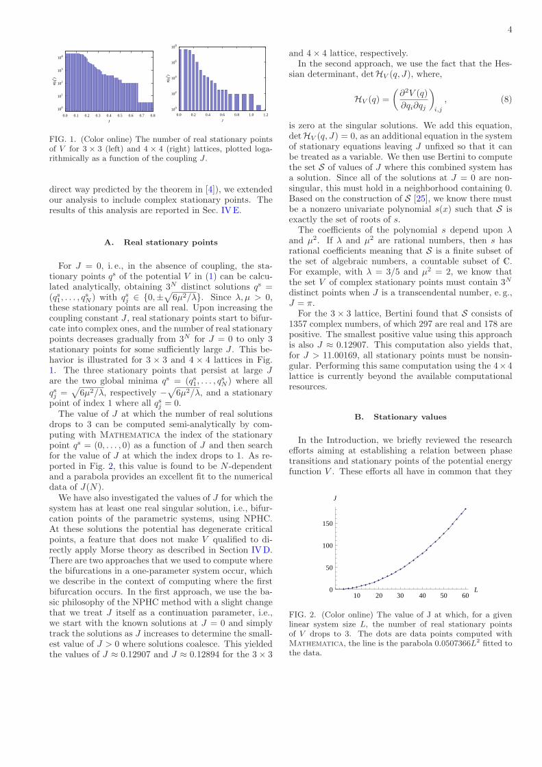
FIG. 1. (Color online) The number of real stationary pointsof V for 3 × 3 (left) and 4 × 4 (right) lattices, plotted loga-rithmically as a function of the coupling J .

direct way predicted by the theorem in [4]), we extendedour analysis to include complex stationary points. Theresults of this analysis are reported in Sec. IV E.

A. Real stationary points

For J = 0, i. e., in the absence of coupling, the sta-tionary points qs of the potential V in (1) can be calcu-lated analytically, obtaining 3N distinct solutions qs =(qs

1, . . . , qsN ) with qs

j ∈ {0,±√

6µ2/λ}. Since λ, µ > 0,these stationary points are all real. Upon increasing thecoupling constant J , real stationary points start to bifur-cate into complex ones, and the number of real stationarypoints decreases gradually from 3N for J = 0 to only 3stationary points for some sufficiently large J . This be-havior is illustrated for 3 × 3 and 4 × 4 lattices in Fig.1. The three stationary points that persist at large Jare the two global minima qs = (qs

1, . . . , qsN ) where all

qsj =

√

6µ2/λ, respectively −√

6µ2/λ, and a stationarypoint of index 1 where all qs

j = 0.The value of J at which the number of real solutions

drops to 3 can be computed semi-analytically by com-puting with Mathematica the index of the stationarypoint qs = (0, . . . , 0) as a function of J and then searchfor the value of J at which the index drops to 1. As re-ported in Fig. 2, this value is found to be N -dependentand a parabola provides an excellent fit to the numericaldata of J(N).

We have also investigated the values of J for which thesystem has at least one real singular solution, i.e., bifur-cation points of the parametric systems, using NPHC.At these solutions the potential has degenerate criticalpoints, a feature that does not make V qualified to di-rectly apply Morse theory as described in Section IVD.There are two approaches that we used to compute wherethe bifurcations in a one-parameter system occur, whichwe describe in the context of computing where the firstbifurcation occurs. In the first approach, we use the ba-sic philosophy of the NPHC method with a slight changethat we treat J itself as a continuation parameter, i.e.,we start with the known solutions at J = 0 and simplytrack the solutions as J increases to determine the small-est value of J > 0 where solutions coalesce. This yieldedthe values of J ≈ 0.12907 and J ≈ 0.12894 for the 3 × 3

and 4 × 4 lattice, respectively.In the second approach, we use the fact that the Hes-

sian determinant, detHV (q, J), where,

HV (q) =

(

∂2V (q)

∂qi∂qj

)

i,j

, (8)

is zero at the singular solutions. We add this equation,detHV (q, J) = 0, as an additional equation in the systemof stationary equations leaving J unfixed so that it canbe treated as a variable. We then use Bertini to computethe set S of values of J where this combined system hasa solution. Since all of the solutions at J = 0 are non-singular, this must hold in a neighborhood containing 0.Based on the construction of S [25], we know there mustbe a nonzero univariate polynomial s(x) such that S isexactly the set of roots of s.

The coefficients of the polynomial s depend upon λand µ2. If λ and µ2 are rational numbers, then s hasrational coefficients meaning that S is a finite subset ofthe set of algebraic numbers, a countable subset of C.For example, with λ = 3/5 and µ2 = 2, we know thatthe set V of complex stationary points must contain 3N

distinct points when J is a transcendental number, e. g.,J = π.

For the 3 × 3 lattice, Bertini found that S consists of1357 complex numbers, of which 297 are real and 178 arepositive. The smallest positive value using this approachis also J ≈ 0.12907. This computation also yields that,for J > 11.00169, all stationary points must be nonsin-gular. Performing this same computation using the 4×4lattice is currently beyond the available computationalresources.

B. Stationary values

In the Introduction, we briefly reviewed the researchefforts aiming at establishing a relation between phasetransitions and stationary points of the potential energyfunction V . These efforts all have in common that they

10 20 30 40 50 60L0

50

100

150

J

FIG. 2. (Color online) The value of J at which, for a givenlinear system size L, the number of real stationary pointsof V drops to 3. The dots are data points computed withMathematica, the line is the parabola 0.0507366L2 fitted tothe data.

5

0.0

1.0

2.0

3.0

4.0

5.0

6.0

-10.0 -8.0 -6.0 -4.0 -2.0 0.0

D

v

0.0

1.0

2.0

3.0

4.0

5.0

6.0

-10.0 -8.0 -6.0 -4.0 -2.0 0.0

D

v

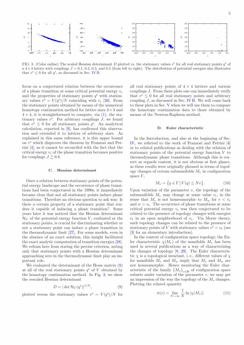
FIG. 3. (Color online) The scaled Hessian determinant D plotted vs. the stationary values vs for all real stationary points qs ofa 4×4 lattice with couplings J = 0.1, 0.2, 0.3, and 0.5 (from left to right). The distribution of potential energies also illustratesthat vs ≤ 0 for all qs, as discussed in Sec. IVB.

focus on a conjectured relation between the occurrenceof a phase transition at some critical potential energy vc

and the properties of stationary points qs with station-ary values vs = V (qs)/N coinciding with vc [26]. Fromthe stationary points obtained by means of the numericalhomotopy continuation method for lattice sizes 3×3 and4 × 4, it is straightforward to compute, via (1), the sta-tionary values vs. For arbitrary couplings J , we foundthat vs ≤ 0 for all stationary points qs. An analyticalcalculation, reported in [9], has confirmed this observa-tion and extended it to lattices of arbitrary sizes. Asexplained in this same reference, it is this upper boundon vs which disproves the theorem by Franzosi and Pet-tini [4], as it cannot be reconciled with the fact that thecritical energy vc of the phase transition becomes positivefor couplings J & 0.8.

C. Hessian determinant

Once a relation between stationary points of the poten-tial energy landscape and the occurrence of phase transi-tions had been conjectured in the 1990s, it immediatelybecame clear that not all stationary points induce phasetransitions. Therefore an obvious question to ask was: Isthere a certain property of a stationary point that ren-ders it capable of inducing a phase transition? Someyears later it was noticed that the Hessian determinantHV of the potential energy function V , evaluated at thestationary points, is crucial for discriminating whether ornot a stationary point can induce a phase transition inthe thermodynamic limit [27]. For some models, even inthe absence of an exact solution, this insight facilitatedthe exact analytic computation of transition energies [28].We refrain here from stating the precise criterion, notingonly that stationary points with a Hessian determinantapproaching zero in the thermodynamic limit play an im-portant role.

We evaluated the determinant of the Hesse matrix (8)at all of the real stationary points qs of V obtained bythe homotopy continuation method. In Fig. 3, we showthe rescaled Hessian determinant

D = |detHV (qs)|1/N , (9)

plotted versus the stationary values vs = V (qs)/N for

all real stationary points of 4 × 4 lattices and variouscouplings J . From these plots one can immediately verifythat vs ≤ 0 for all real stationary points and arbitrarycoupling J , as discussed in Sec. IVB. We will come backto these plots in Sec. V when we will use them to comparethe homotopy continuation data to those obtained bymeans of the Newton-Raphson method.

D. Euler characteristic

In the Introduction, and also at the beginning of Sec.IV, we referred to the work of Franzosi and Pettini [4]or to related publications as dealing with the relation ofstationary points of the potential energy function V tothermodynamic phase transitions. Although this is cor-rect as regards content, it is not obvious at first glance,as these results were originally phrased in terms of topol-ogy changes of certain submanifolds Mv in configurationspace Γ,

Mv ={

q ∈ Γ∣

∣ V (q) ≤ Nv}

. (10)

Upon variation of the parameter v, the topology of thesubmanifolds Mv may change at some value vt, in thesense that Mv is not homeomorphic to Mw for v < vt

and w > vt. The occurrence of phase transitions at somecritical potential energy vc was then conjectured to berelated to the presence of topology changes with energiesvt in an open neighborhood of vc. Via Morse theory,such topology changes can be related to the presence ofstationary points of V with stationary values vs = vt (see[3] for an elementary introduction).

In the context of configuration space topology, the Eu-ler characteristic χ(Mv) of the manifolds Mv has beenused in several publications as a way of characterizingthe changes of topology [8, 29]. The Euler characteris-tic χ is a topological invariant, i. e., different values of χfor manifolds Mv and Mw imply that Mv and Mw arenot homeomorphic. Hence monitoring the Euler char-acteristic of the family {Mv}v∈R

of configuration spacesubsets under variation of the parameter v, we may getan impression of the way the topology of the Mv changes.Plotting the related quantity

σ(v) = limN→∞

1

Nln |χ(Mv)| (11)

6

0.0

0.1

0.2

0.3

0.4

0.5

0.6

0.7

0.8

-10 -8 -6 -4 -2 0

ln|χ

| /N

v

0.0

0.1

0.2

0.3

0.4

0.5

0.6

0.7

0.8

-10 -8 -6 -4 -2 0

ln|χ

| /N

v

0.0

0.1

0.2

0.3

0.4

0.5

0.6

0.7

0.8

-10 -8 -6 -4 -2 0

ln|χ

| /N

v

0.0

0.1

0.2

0.3

0.4

0.5

0.6

0.7

0.8

-10 -8 -6 -4 -2 0

ln|χ

| /N

v

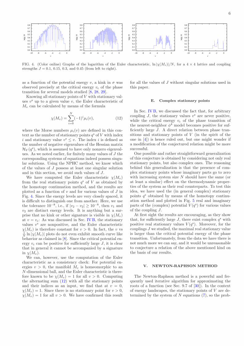
FIG. 4. (Color online) Graphs of the logarithm of the Euler characteristic, ln |χ(Mv)|/N , for a 4 × 4 lattice and couplingstrengths J = 0.1, 0.15, 0.3, and 0.45 (from left to right).

as a function of the potential energy v, a kink in σ wasobserved precisely at the critical energy vc of the phasetransition for several models studied [8, 28, 29].

Knowing all stationary points of V with stationary val-ues vs up to a given value v, the Euler characteristic ofMv can be calculated by means of the formula

χ(Mv) =N

∑

i=0

(−1)iµi(v), (12)

where the Morse numbers µi(v) are defined in this con-text as the number of stationary points qs of V with indexi and stationary value vs ≤ v. The index i is defined asthe number of negative eigenvalues of the Hessian matrixHV (qs), which is assumed to have only nonzero eigenval-ues. As we noted earlier, for finitely many values of J thecorresponding systems of equations indeed possess singu-lar solutions. Using the NPHC method, we know whichof the values of J possess at least one singular solutionand in this section, we avoid such values of J .

We have computed the Euler characteristic χ(Mv)from the real stationary points qs of V as obtained bythe homotopy continuation method, and the results areplotted as a function of v and for various values of J inFig. 4. Since the energy levels are very closely spaced, itis difficult to distinguish one from another. Here, we usethe tolerance 10−8, i.e., if |v2 − v2| ≥ 10−8, then v1 andv2 are distinct energy levels. It is anything but a sur-prise that no kink or other signature is visible in χ(Mv)at v = vc: As was discussed in Sec. IVB, the stationaryvalues vs are nonpositive, and the Euler characteristicχ(Mv) is therefore constant for v > 0. In fact, the v vs1N ln |χ(Mv)| plots do not even exhibit smooth curve likebehavior as claimed in [8]. Since the critical potential en-ergy vc can be positive for sufficiently large J , it is clearthat in general it cannot be accompanied by a signaturein χ(Mv).

We can, however, use the computation of the Eulercharacteristic as a consistency check: For potential en-ergies v > 0, the manifold Mv is homeomorphic to anN -dimensional ball, and the Euler characteristic is there-fore known to be χ(Mv) = 1 for all v > 0. Computingthe alternating sum (12) with all the stationary pointsand their indices as an input, we find that at v = 0,χ(Mv) = 1. Since there is no stationary point for v > 0,χ(Mv) = 1 for all v > 0. We have confirmed this result

for all the values of J without singular solutions used inthis paper.

E. Complex stationary points

In Sec. IV B, we discussed the fact that, for arbitrarycoupling J , the stationary values vs are never positive,while the critical energy vc of the phase transition ofthe nearest-neighbor φ4 model becomes positive for suf-ficiently large J . A direct relation between phase tran-sitions and stationary points of V (in the spirit of theone in [4]) is hence ruled out, but one might wonder ifa modification of the conjectured relation might be moresuccessful.

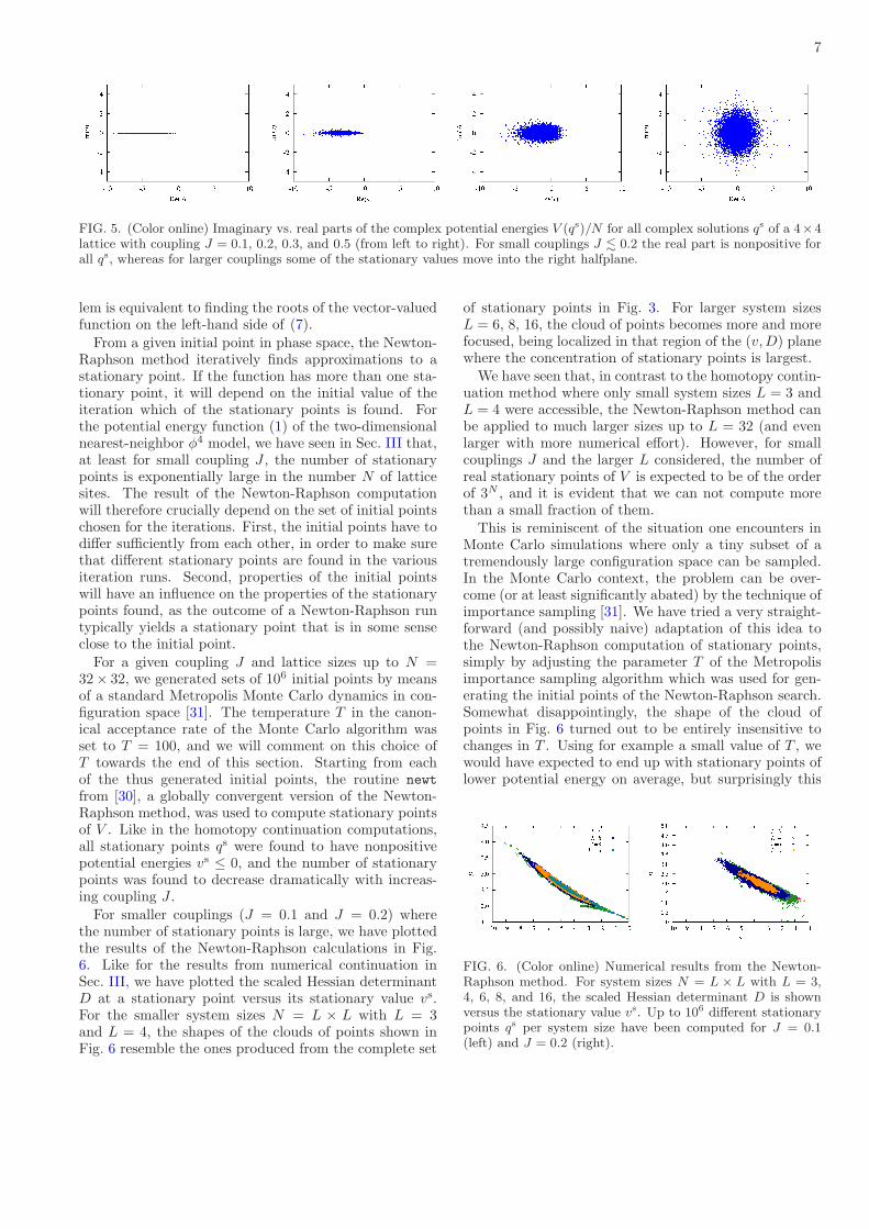
One possible and rather straightforward generalizationof this conjecture is obtained by considering not only realstationary points, but also complex ones. The reasoningbehind this generalization is that the presence of com-plex stationary points whose imaginary parts go to zerowith increasing system size N should have the same (orat least a similar) effect on the thermodynamic proper-ties of the system as their real counterparts. To test thisidea, we have used the (in general complex) stationarypoints qs obtained by means of the homotopy continu-ation method and plotted in Fig. 5 real and imaginaryparts of the (complex) potential V (qs) for various valuesof the coupling J .

At first sight the results are encouraging, as they showthat, for sufficiently large J , there exist complex qs withpositive real stationary values V (qs). Moreover, for thecouplings J we studied, the maximal real stationary valueis larger than the critical potential energy of the phasetransition. Unfortunately, from the data we have there isnot much more we can say, and it would be unreasonableto conjecture a relation of the above mentioned kind onthe basis of our results.

V. NEWTON-RAPHSON METHOD

The Newton-Raphson method is a powerful and fre-quently used iterative algorithm for approximating theroots of a function (see Sec. 9.7 of [30]). In the contextof energy landscapes, the stationary points of V are de-termined by the system of N equations (7), so the prob-

7

FIG. 5. (Color online) Imaginary vs. real parts of the complex potential energies V (qs)/N for all complex solutions qs of a 4×4lattice with coupling J = 0.1, 0.2, 0.3, and 0.5 (from left to right). For small couplings J . 0.2 the real part is nonpositive forall qs, whereas for larger couplings some of the stationary values move into the right halfplane.

lem is equivalent to finding the roots of the vector-valuedfunction on the left-hand side of (7).

From a given initial point in phase space, the Newton-Raphson method iteratively finds approximations to astationary point. If the function has more than one sta-tionary point, it will depend on the initial value of theiteration which of the stationary points is found. Forthe potential energy function (1) of the two-dimensionalnearest-neighbor φ4 model, we have seen in Sec. III that,at least for small coupling J , the number of stationarypoints is exponentially large in the number N of latticesites. The result of the Newton-Raphson computationwill therefore crucially depend on the set of initial pointschosen for the iterations. First, the initial points have todiffer sufficiently from each other, in order to make surethat different stationary points are found in the variousiteration runs. Second, properties of the initial pointswill have an influence on the properties of the stationarypoints found, as the outcome of a Newton-Raphson runtypically yields a stationary point that is in some senseclose to the initial point.

For a given coupling J and lattice sizes up to N =32× 32, we generated sets of 106 initial points by meansof a standard Metropolis Monte Carlo dynamics in con-figuration space [31]. The temperature T in the canon-ical acceptance rate of the Monte Carlo algorithm wasset to T = 100, and we will comment on this choice ofT towards the end of this section. Starting from eachof the thus generated initial points, the routine newt

from [30], a globally convergent version of the Newton-Raphson method, was used to compute stationary pointsof V . Like in the homotopy continuation computations,all stationary points qs were found to have nonpositivepotential energies vs ≤ 0, and the number of stationarypoints was found to decrease dramatically with increas-ing coupling J .

For smaller couplings (J = 0.1 and J = 0.2) wherethe number of stationary points is large, we have plottedthe results of the Newton-Raphson calculations in Fig.6. Like for the results from numerical continuation inSec. III, we have plotted the scaled Hessian determinantD at a stationary point versus its stationary value vs.For the smaller system sizes N = L × L with L = 3and L = 4, the shapes of the clouds of points shown inFig. 6 resemble the ones produced from the complete set

of stationary points in Fig. 3. For larger system sizesL = 6, 8, 16, the cloud of points becomes more and morefocused, being localized in that region of the (v,D) planewhere the concentration of stationary points is largest.

We have seen that, in contrast to the homotopy contin-uation method where only small system sizes L = 3 andL = 4 were accessible, the Newton-Raphson method canbe applied to much larger sizes up to L = 32 (and evenlarger with more numerical effort). However, for smallcouplings J and the larger L considered, the number ofreal stationary points of V is expected to be of the orderof 3N , and it is evident that we can not compute morethan a small fraction of them.

This is reminiscent of the situation one encounters inMonte Carlo simulations where only a tiny subset of atremendously large configuration space can be sampled.In the Monte Carlo context, the problem can be over-come (or at least significantly abated) by the technique ofimportance sampling [31]. We have tried a very straight-forward (and possibly naive) adaptation of this idea tothe Newton-Raphson computation of stationary points,simply by adjusting the parameter T of the Metropolisimportance sampling algorithm which was used for gen-erating the initial points of the Newton-Raphson search.Somewhat disappointingly, the shape of the cloud ofpoints in Fig. 6 turned out to be entirely insensitive tochanges in T . Using for example a small value of T , wewould have expected to end up with stationary points oflower potential energy on average, but surprisingly this

FIG. 6. (Color online) Numerical results from the Newton-Raphson method. For system sizes N = L × L with L = 3,4, 6, 8, and 16, the scaled Hessian determinant D is shownversus the stationary value vs. Up to 106 different stationarypoints qs per system size have been computed for J = 0.1(left) and J = 0.2 (right).

8

was not the case.There are other, more involved ways of how one could

shift the search of stationary points to higher or lower po-tential energies, but we have not yet implemented suchrefinements. One could, for example, use a more ad-vanced search routine (like the OPTIM program package[32]) which allows one to search for stationary points ofa given index, i. e., of a given number of negative eigen-values of the Hessian at the stationary point. Since theindex of a stationary point and its potential energy areexpected to be correlated, such a routine should find sta-tionary points of low energy when searching for smallindices, and vice versa.

VI. CONCLUSIONS

Two numerical methods for the computation of sta-tionary points of multivariate functions were discussed inthis article: the numerical polynomial homotopy contin-uation method (NPHC) and a globally-convergent vari-ant of the Newton-Raphson method. We applied bothmethods to the potential energy function V of the two-dimensional nearest-neighbor φ4 model on L × L squarelattices. The NPHC method allows one to obtain all sta-tionary points of V , but is limited to system sizes up to4 × 4 with the computational resources we had at ourdisposal. With the Newton-Raphson method we havecomputed stationary points for larger lattices of up to32×32 sites, but only a small subset of all the stationarypoints of such a large system could be obtained.

The motivation for this type of study originates from anumber of conjectures relating the stationary points of Vto the occurrence of phase transitions in the thermody-namic limit. These conjectures refer to certain quantitieswhich can be computed from the stationary points of V ,like their potential energies, their Hessian determinants,and the Euler characteristic of the underlying potentialenergy manifolds in configuration space. We have cal-culated these and a few other quantities from the sta-tionary points of the φ4 model obtained with NPHC andNewton-Raphson, but—contrary to what the conjecturessuggest—no sign of the phase transition of the model wasfound. This failure and its consequences, including thefalsification of a theorem allegedly proven in [4], was dis-cussed in a Letter [9].

The NPHC results for the nearest-neighbor φ4 model

on a 4 × 4 lattice can be overviewed as follows:

1. The number of real stationary points decreasesfrom 3N for J = 0 to only 3 with increasing J

2. Singular solutions occur only for finitely many val-ues of J .

3. The stationary values vs are all nonpositive for ar-bitrary couplings J .

4. The Euler characteristic, computed as the alternat-ing sum of the Morse numbers, confirms the cor-rect and complete computation of all the stationarypoints.

5. Unlike real stationary points, complex stationarypoints of V can have positive stationary values, butwe were unable to identify a relation between thesepositive values and the positive phase transition en-ergy of the φ4 model for larger J .

Since the Newton-Raphson method yields only a sub-set of all the stationary points, we compared these resultsfor system sizes up to 16 × 16 to those obtained by theNPHC method for 4 × 4 lattices. For this comparisonwe chose plots of the rescaled Hessian determinant D asdefined in (9) vs. the potential energy v. A comparisonof different lattice sizes is of course problematic, but ageneral trend can be deduced: For system sizes 8 × 8and larger, the number of stationary points becomes ingeneral so large that only that region in the (D, v)-planeis explored where the (strongly peaked) density of sta-tionary points is the highest. Importance sampling mayprovide a way out of these difficulties, but we have notyet implemented such a scheme.

ACKNOWLEDGMENTS

D.M. acknowledges support by the U.S. Departmentof Energy under contract DE-FG02-85ER40237 and bythe Science Foundation Ireland grant 08/RFP/PHY1462.J.D.H. acknowledges support by the U.S. National Sci-ence Foundation under grants DMS-0915211 and DMS-1114336. M.K. acknowledges support by the Incentive

Funding for Rated Researchers programme of the Na-tional Research Foundation of South Africa.

[1] D. J. Wales, Energy Landscapes (Cambridge UniversityPress, Cambridge, 2004).

[2] L. Casetti, M. Pettini, and E. G. D. Cohen, “Geometricapproach to Hamiltonian dynamics and statistical me-chanics,” Phys. Rep., 337, 237–341 (2000).

[3] M. Kastner, “Phase transitions and configuration spacetopology,” Rev. Mod. Phys., 80, 167–187 (2008).

[4] R. Franzosi and M. Pettini, “Theorem on the origin of

phase transitions,” Phys. Rev. Lett., 92, 060601 (2004);R. Franzosi, M. Pettini, and L. Spinelli, “Topology andphase transitions I. Preliminary results,” Nuclear Phys.B, 782, 189–218 (2007).

[5] F. Baroni, Transizioni di fase e topologia dello spaziodelle configurazioni di modelli di campo medio, Master’sthesis, Universita degli Studi di Firenze (2002); D. A.Garanin, R. Schilling, and A. Scala, “Saddle index prop-

9

erties, singular topology, and its relation to thermody-namic singularities for a φ4 mean-field model,” Phys.Rev. E, 70, 036125 (2004); A. Andronico, L. Angelani,G. Ruocco, and F. Zamponi, “Topological properties ofthe mean-field φ4 model,” ibid., 70, 041101 (2004).

[6] M. Kastner, “Unattainability of a purely topologicalcriterion for the existence of a phase transition fornon-confining potentials,” Phys. Rev. Lett., 93, 150601(2004).

[7] Note that most exactly solvable models with short-range interactions, like for example the two-dimensionalnearest-neighbor Ising model, have a discrete configura-tion space and the energy landscape techniques we areinterested in do not apply.

[8] R. Franzosi, M. Pettini, and L. Spinelli, “Topology andphase transitions: Paradigmatic evidence,” Phys. Rev.Lett., 84, 2774–2777 (2000).

[9] M. Kastner and D. Mehta, “Phase transitions detachedfrom stationary points of the energy landscape,” Phys.Rev. Lett., 107, 160602 (2011).

[10] Our definition of V coincides with the one in [14], butdiffers from [8] by a factor 1/6 in the quartic term. Judg-ing from the critical temperatures and energies reportedin the latter, as well as from their reference to [14], weassume that there is a misprint in [8]. For the main con-clusions in [9] and in the present article, the precise valuesof any of the constants are not crucial.

[11] A. Milchev, D. W. Heermann, and K. Binder, “Finite-size scaling snalysis of the φ4 field theory on the squarelattice,” J. Stat. Phys., 44, 749–784 (1986).

[12] M. Kastner, “Topological approach to phase transitionsand inequivalence of statistical ensembles,” Physica A,359, 447–454 (2006).

[13] D. Ruelle, Statistical Mechanics: Rigorous Results (Ben-jamin, Reading, 1969), Chapter 2.4.

[14] R. Franzosi, L. Casetti, L. Spinelli, and M. Pettini,“Topological aspects of geometrical signatures of phasetransitions,” Phys. Rev. E, 60, R5009–R5012 (1999).

[15] B. Roth, “A generalization of Burmester theory: Nine-point path generation of geared five-bar mechanisms withgear ratio plus and minus one.” Ph.D. Thesis, ColumbiaUniversity (1962).

[16] E. L. Allgower and K. Georg, Introduction to NumericalContinuation Methods (John Wiley & Sons, New York,1979).

[17] A. J. Sommese and C. W. Wampler, The Numerical So-lution of Systems of Polynomials Arising in Engineeringand Science (World Scientific, Singapore, 2005).

[18] T. Y. Li, “Solving polynomial systems by the homotopycontinuation method,” Handbook of Numerical Analysis,XI, 209–304 (2003).

[19] J. Verschelde, “Algorithm 795: PHCpack: a general-purpose solver for polynomial systems by homotopy con-tinuation,” ACM Trans. Math. Soft., 25 (1999).

[20] T. L. Lee, T. Y. Li, and C. H. Tsai, “HOM4PS-2.0, asoftware package for solving polynomial systems by thepolyhedral homotopy continuation method,” Computing,83, 109–133 (2008).

[21] D. J. Bates, J. D. Hauenstein, A. J. Sommese, and C. W.Wampler, Available at www.nd.edu/~sommese/bertini.

[22] J. D. Hauenstein and F. Sottile, “alphaCertified: Certify-ing solutions to polynomial systems,” To appear in ACM

Trans. Math. Softw. (2012).[23] J. D. Hauenstein and F. Sottile, Available at

www.math.tamu.edu/~sottile/research/stories/

alphaCertified.[24] D. Mehta, Lattice vs. Continuum: Landau Gauge Fix-

ing and ’t Hooft-Polyakov Monopoles, Ph.D. thesis, Uni-versity of Adelaide (2009); D. Mehta, A. Sternbeck,L. von Smekal, and A. G. Williams, “Lattice Landaugauge and algebraic geometry,” PoS, QCD-TNT09, 025(2009); D. Mehta, “Finding all the stationary pointsof a potential energy landscape via numerical polyno-mial homotopy continuation method,” Phys. Rev., E84,025702 (2011); “Numerical polynomial homotopy con-tinuation method and string vacua,” Adv. High EnergyPhys., 2011, 263937.

[25] The set S is a non-dense constructible algebraic subsetof C and thus must be a proper algebraic subset of C.

[26] In contrast to other approaches which focus on what iscalled the underlying stationary points; see [33].

[27] M. Kastner, S. Schreiber, and O. Schnetz, “Phase tran-sitions from saddles of the potential energy landscape,”Phys. Rev. Lett., 99, 050601 (2007); M. Kastner andO. Schnetz, “Phase transitions induced by saddle pointsof vanishing curvature,” 100, 160601 (2008); M. Kast-ner, O. Schnetz, and S. Schreiber, “Nonanalyticities ofthe entropy induced by saddle points of the potentialenergy landscape,” J. Stat. Mech. Theory Exp., 2008,P04025 (2008).

[28] C. Nardini and L. Casetti, “Energy landscape and phasetransitions in the self-gravitating ring model,” Phys. Rev.E, 80, 060103(R) (2009); M. Kastner, “Stationary pointapproach to the phase transition of the classical XYchain with power law interactions,” 83, 031114 (2011).

[29] L. Casetti, E. G. D. Cohen, and M. Pettini, “Exact resulton topology and phase transitions at any finite N ,” Phys.Rev. E, 65, 036112 (2002); L. Casetti, M. Pettini, andE. G. D. Cohen, “Phase transitions and topology changesin configuration space,” J. Stat. Phys., 111, 1091–1123(2003); L. Angelani, L. Casetti, M. Pettini, G. Ruocco,and F. Zamponi, “Topological signature of first-orderphase transitions in a mean-field model,” Europhys.Lett., 62, 775–781 (2003); D. Mehta and M. Kastner,“Stationary point analysis of the one-dimensional latticeLandau gauge fixing functional, aka random phase XYHamiltonian,” Ann. Phys. (New York), 326, 1425–1440.

[30] W. H. Press, S. A Teukolsky, W. T. Vetterling, and B. P.Flannery, Numerical Recipes in C: The Art of ScientificComputing, 2nd ed. (Cambridge University Press, Cam-bridge, 1992).

[31] M. Kastner, “Monte Carlo methods in statistical physics:Mathematical foundations and strategies,” Commun.Nonlinear Sci. Numer. Simul., 15, 1589–1602 (2010).

[32] D. Wales, “OPTIM: A program for optimizing geometriesand calculating reaction pathways,” Available at http://www-wales.ch.cam.ac.uk/OPTIM/.

[33] L. Angelani, G. Ruocco, and F. Zamponi, “Relation-ship between phase transitions and topological changesin one-dimensional models,” Phys. Rev. E, 72, 016122(2005); L. Angelani and G. Ruocco, “Role of saddles intopologically driven phase transitions: The case of thed-dimensional spherical model,” 77, 052101 (2008).