Emission and Absorption - mps.mpg.de · classical radiation damping constant ... Profile function...
35
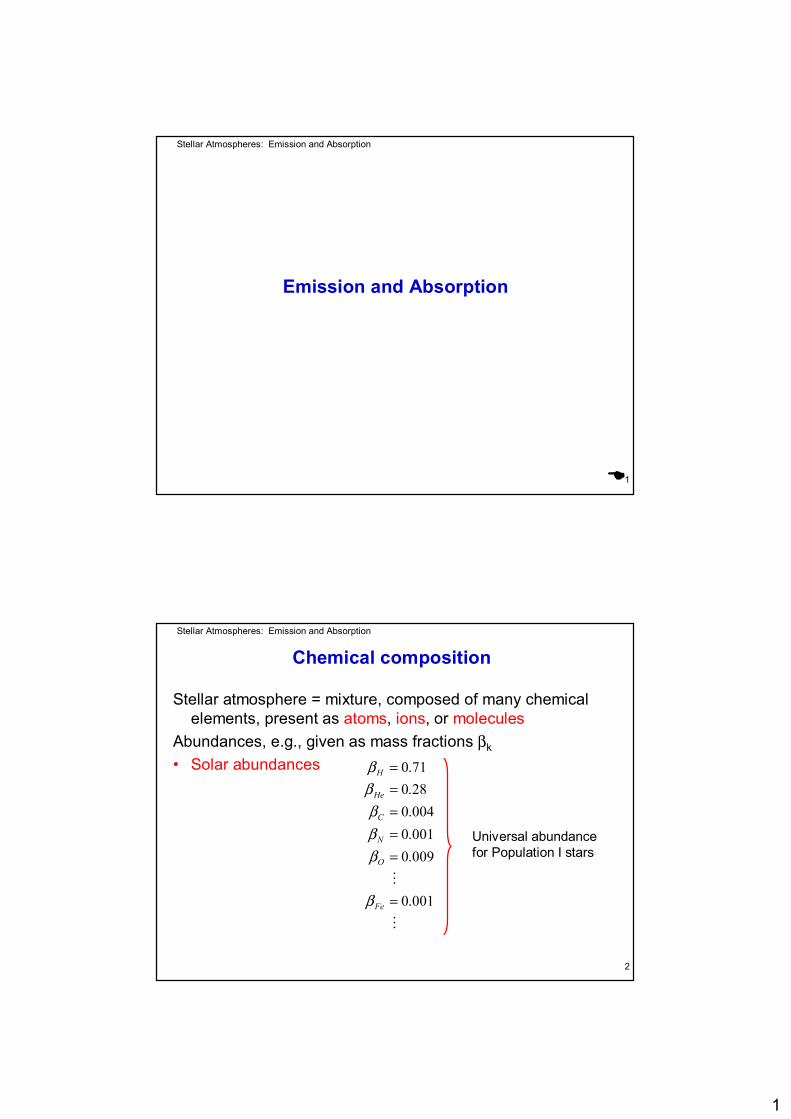
1 Stellar Atmospheres: Emission and Absorption 1 Emission and Absorption Stellar Atmospheres: Emission and Absorption 2 Chemical composition Stellar atmosphere = mixture, composed of many chemical elements, present as atoms, ions, or molecules Abundances, e.g., given as mass fractions β k • Solar abundances M M 001 . 0 009 . 0 001 . 0 004 . 0 28 . 0 71 . 0 = = = = = = Fe O N C He H β β β β β β Universal abundance for Population I stars
Transcript of Emission and Absorption - mps.mpg.de · classical radiation damping constant ... Profile function...
1
Stellar Atmospheres: Emission and Absorption
1
Emission and Absorption
Stellar Atmospheres: Emission and Absorption
2
Chemical composition
Stellar atmosphere = mixture, composed of many chemicalelements, present as atoms, ions, or molecules
Abundances, e.g., given as mass fractions βk
• Solar abundances
M
M
001.0
009.0001.0004.028.071.0
=
=====
Fe
O
N
C
He
H
β
βββ
ββ
Universal abundance for Population I stars
2
Stellar Atmospheres: Emission and Absorption
3
Chemical composition
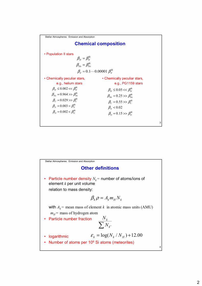
• Population II stars
• Chemically peculiar stars, e.g., helium stars
• Chemically peculiar stars, e.g., PG1159 stars
0.1 0.00001
H H
He He
Z Z
β ββ ββ β
=
=
= L
0.0020.964
0.029
0.003
0.002
H H
He He
C C
N N
O O
β ββ ββ ββ ββ β
≤ <<
= >>
= >>
= ≈
= <
0.05
0.25
0.550.02
0.15
H H
He He
C C
N
O O
β ββ ββ βββ β
≤ <<
= >>
= >><
= >>
Stellar Atmospheres: Emission and Absorption
4
Other definitions
• Particle number density Nk = number of atoms/ions of element k per unit volumerelation to mass density:
with Ak = mean mass of element k in atomic mass units (AMU)mH = mass of hydrogen atom
• Particle number fraction
• logarithmic• Number of atoms per 106 Si atoms (meteorites)
kHkk NmA=ρβ
∑ ′k
k
NN
00.12)/log( += Hkk NNε
3
Stellar Atmospheres: Emission and Absorption
5
The model atom
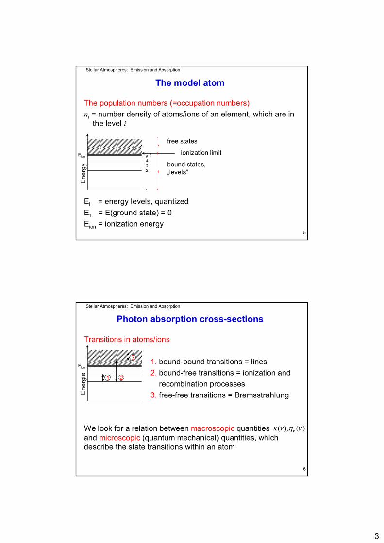
The population numbers (=occupation numbers)ni = number density of atoms/ions of an element, which are in
the level i
Ei = energy levels, quantizedE1 = E(ground state) = 0Eion = ionization energy
bound states, „levels“
free states
ionization limit
1
65432
Ene
rgy
Eion
Stellar Atmospheres: Emission and Absorption
6
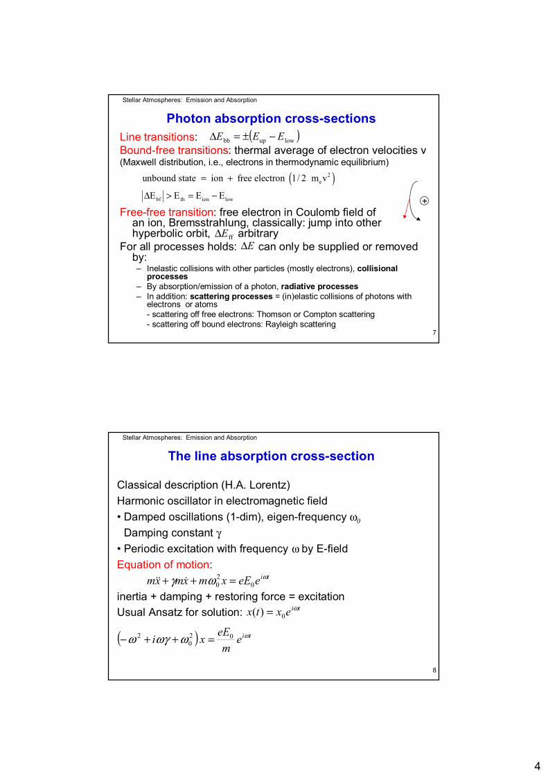
Transitions in atoms/ions
1. bound-bound transitions = lines2. bound-free transitions = ionization and
recombination processes3. free-free transitions = Bremsstrahlung
We look for a relation between macroscopic quantities and microscopic (quantum mechanical) quantities, whichdescribe the state transitions within an atom
Ene
rgie
Eion
Photon absorption cross-sections
1 2
3
)(),( νηνκ ν
4
Stellar Atmospheres: Emission and Absorption
7
Line transitions:Bound-free transitions: thermal average of electron velocities v(Maxwell distribution, i.e., electrons in thermodynamic equilibrium)
Free-free transition: free electron in Coulomb field of an ion, Bremsstrahlung, classically: jump into other hyperbolic orbit, arbitrary
For all processes holds: can only be supplied or removed by:– Inelastic collisions with other particles (mostly electrons), collisional
processes– By absorption/emission of a photon, radiative processes– In addition: scattering processes = (in)elastic collisions of photons with
electrons or atoms- scattering off free electrons: Thomson or Compton scattering- scattering off bound electrons: Rayleigh scattering
Photon absorption cross-sections
ffE∆E∆
( )2e
bf th ion low
unbound state ion free electron 1/ 2 m v
E E E E
= +
∆ > = −
( )lowupbb EEE −±=∆
+
Stellar Atmospheres: Emission and Absorption
8
The line absorption cross-section
Classical description (H.A. Lorentz)Harmonic oscillator in electromagnetic field• Damped oscillations (1-dim), eigen-frequency ω0
Damping constant γ• Periodic excitation with frequency ω by E-fieldEquation of motion:
inertia + damping + restoring force = excitationUsual Ansatz for solution:
tieeExmxmxm ωωγ 020 =++ &&&
tiextx ω0)( =
( ) tiem
eExi ωωωγω 020
2 =++−
5
Stellar Atmospheres: Emission and Absorption
9
The line absorption cross-section
( ) ( )
22
3
2 22 20 0
2 2 2 2 2 2 2 2 2 20 0
22 2 4 2 2 52 2 60 02 2 20
2 2 2
Electrodynamics: 2 ( )3
( ) cos ( )sin( ) ( )
2cos co
radiated p
s sin s
ower
in
ep(t) xc
eEx(t) t tm
eE(x(t)) t t t tm N N N
ω ω γωω ω ω ωω ω ω γ ω ω ω γ
ω ω ω γ ω ω ω γ ωω ω ω ω
=
−= − + − − + − + − − = + +
&&
&&
&&
( )
( )( )
2 2 00
02 20
2 200
2 2 2 2 20
2 20 0
2 2 2 2 2 2 2 2 2 20 0
1
expand ( )
real part Re cos sin( ) ( )
− + + =
= ⋅− +
− −= ⋅
− +
−= + − + − +
i t
t
ti
i
eEi x(t) em
eEx(t) em i
eEx(t) em
eE(x(t)) t t
i
m
ω
ω
ω
ω ωγ ω
ω ω ωγ
ω ω ωγω ω ω γ
ω ω γωω ωω ω ω γ ω ω ω γ
Stellar Atmospheres: Emission and Absorption
10
The line absorption coss-section
( )( )( )
( )
2 2
22 2 2 2 2202 0
222 2 2 20
2 42 0
22 2 2
2
0
3
2
average over one period
power, averaged ove
cos sin 1/ 2,
r one
cos sin 0
1(2
1
perio
(2
3
d
2 (
= = =
− +
= − +
=
=
− +
&
&
&
&&
&ep x
t t t t
eEx)
E)m
c
m
ex
ω ω ω ω
ω ω γ ωω
ω ω γ ω
ωω ω γ ω
( )
( )
4 20
2
4 22 04
22 2 2 2
3
4
22 2 2
3
0
0
2
2
C=normalization constant ( )3
( ) profi
)3
le functi
( ) /
/
n( 2
o )
= = /2
=−
− +
+
=
C
e
e Epm c
C
Em c
ωω ω γ
ν ω π
νϕ νν ν γ π ν
ω
ϕ ν
6
Stellar Atmospheres: Emission and Absorption
11
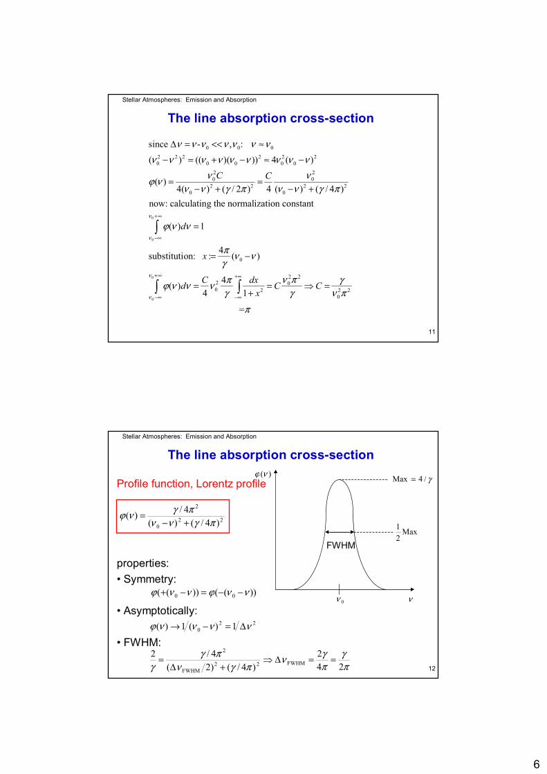
The line absorption cross-section
0
0
0 0 02 2 2 2 2 20 0 0 0 0
2 20 0
2 2 2 20 0
0
since - , :
( ) (( )( )) 4 ( )
( )4( ) ( / 2 ) 4 ( ) ( / 4 )
now: calculating the normalization constant
( ) 1
4substitution: : ( )
(
+∞
−∞
∆ = << ≈
− = + − ≈ −
= =− + − +
=
= −
∫
C C
d
x
ν
ν
ν ν ν ν ν ν νν ν ν ν ν ν ν ν ν
ν νϕ νν ν γ π ν ν γ π
ϕ ν ν
π ν νγ
ϕ0
0
2 22 00 2 2 2
0
4)4 1
=
+∞ +∞
−∞ −∞
= = ⇒ =+∫ ∫
C dxd C Cx
ν
ν
ν ππ γν ν νγ γ ν π
π
Stellar Atmospheres: Emission and Absorption
12
Profile function, Lorentz profile
properties:• Symmetry:
• Asymptotically:
• FWHM:
The line absorption cross-section
220
2
)4/()(4/)(
πγννπγνϕ
+−=
γ/4Max =
Max21
0ν ν
)(νϕ
FWHM
))(())(( 00 ννϕννϕ −−=−+
220 1)(1)( ννννϕ ∆=−→
πγ
πγν
πγνπγ
γ 242
)4/()2(4/2
FWHM22FWHM
2
==∆⇒+∆
=
7
Stellar Atmospheres: Emission and Absorption
13
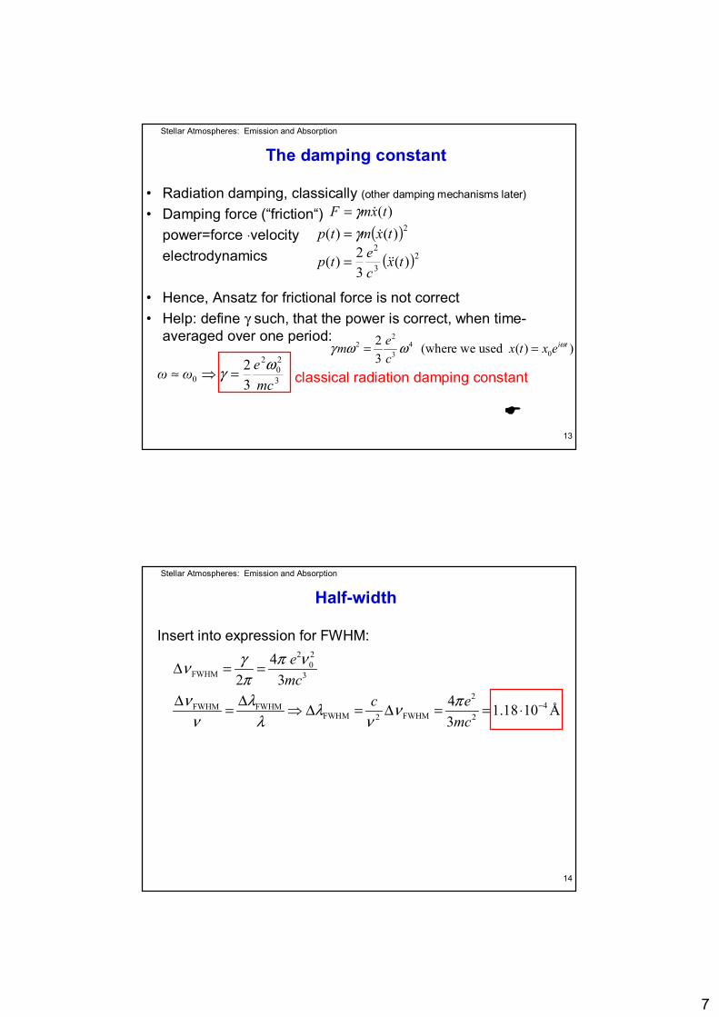
The damping constant
• Radiation damping, classically (other damping mechanisms later)
• Damping force (“friction“)power=force ⋅velocityelectrodynamics
• Hence, Ansatz for frictional force is not correct• Help: define γ such, that the power is correct, when time-
averaged over one period:
classical radiation damping constant
)(txmF &γ=( )2)()( txmtp &γ=
( )23
2
)(32)( tx
cetp &&=
22 4
03
2 (where we used ( ) )3
= = i tem x t x ec
ωγ ω ω
3
20
2
0 32
mceωω ωγ =⇒≈
Stellar Atmospheres: Emission and Absorption
14
Half-width
Insert into expression for FWHM:2 2
0FWHM 3
24FWHM FWHM
FWHM FWHM2 2
42 3
4 1.18 10 Å3
emc
c emc
π νγνπ
ν λ πλ νν λ ν
−
∆ = =
∆ ∆= ⇒ ∆ = ∆ = = ⋅
8
Stellar Atmospheres: Emission and Absorption
15
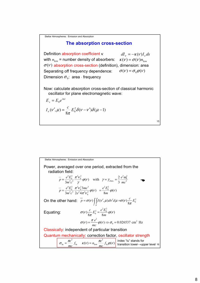
The absorption cross-section
Definition absorption coefficient κwith nlow = number density of absorbers:
absorption cross-section (definition), dimension: areaSeparating off frequency dependence: Dimension : area ⋅ frequency
Now: calculate absorption cross-section of classical harmonicoscillator for plane electromagnetic wave:
dsIdI νν νκ )(−=low)()( nνσνκ =
)(νσ)()( 0 νϕσνσ =
0σ
)1()(8
),( 20
0
−′−=′
=
µδννδπ
µνν
ω
EcI
eEE tix
Stellar Atmospheres: Emission and Absorption
16
Power, averaged over one period, extracted from the radiation field:
On the other hand:
Equating:
Classically: independent of particular transitionQuantum mechanically: correction factor, oscillator strength
4 2 2 2 2 20 0 0
class.2 3 3
4 2 2 2 3 2 20 0 0
2 3 2 2 20
2( ) with 3 3
3 ( ) ( )3 2 4 8
= = =
= =
e E epm c mce E mc e Epm c e m
π ν ωϕ ν γ γγ
π ν ϕ ν ϕ νπ ν
20
2 22 00
22
0
( ) ( , ) ( )8
( ) ( )8 8
( ) ( ) 0.026537 cm Hz
cp I d d E
e Ec Em
emc
ν µ
σ ν ν µ ν µ σ νπ
σ ν ϕ νππσ ν ϕ ν σ
′
′ ′= =
=
= ⇒ =
∫ ∫
)()( lu
2
lowlu
2
lu νϕπνκπσ fmcenf
mce ==
index “lu” stands for transition lower→upper level
9
Stellar Atmospheres: Emission and Absorption
17
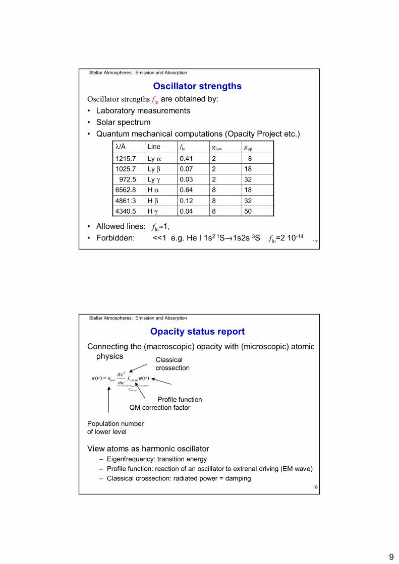
Oscillator strengthsOscillator strengths flu are obtained by:• Laboratory measurements• Solar spectrum• Quantum mechanical computations (Opacity Project etc.)
• Allowed lines: flu≈1, • Forbidden: <<1 e.g. He I 1s2 1S→1s2s 3S flu=2 10-14
3280.12H β4861.3
gupglowfluLineλ/Å
820.41Ly α1215.7
5080.04H γ4340.5
1880.64H α6562.83220.03Ly γ972.51820.07Ly β1025.7
Stellar Atmospheres: Emission and Absorption
18
Opacity status reportConnecting the (macroscopic) opacity with (microscopic) atomic
physics
View atoms as harmonic oscillator– Eigenfrequency: transition energy– Profile function: reaction of an oscillator to extrenal driving (EM wave)– Classical crossection: radiated power = damping
,
2
low low,up( ) ( )
low up
en fmc
σ
πκ ν ϕ ν=1442443
Population number of lower level
QM correction factorProfile function
Classical crossection
10
Stellar Atmospheres: Emission and Absorption
19
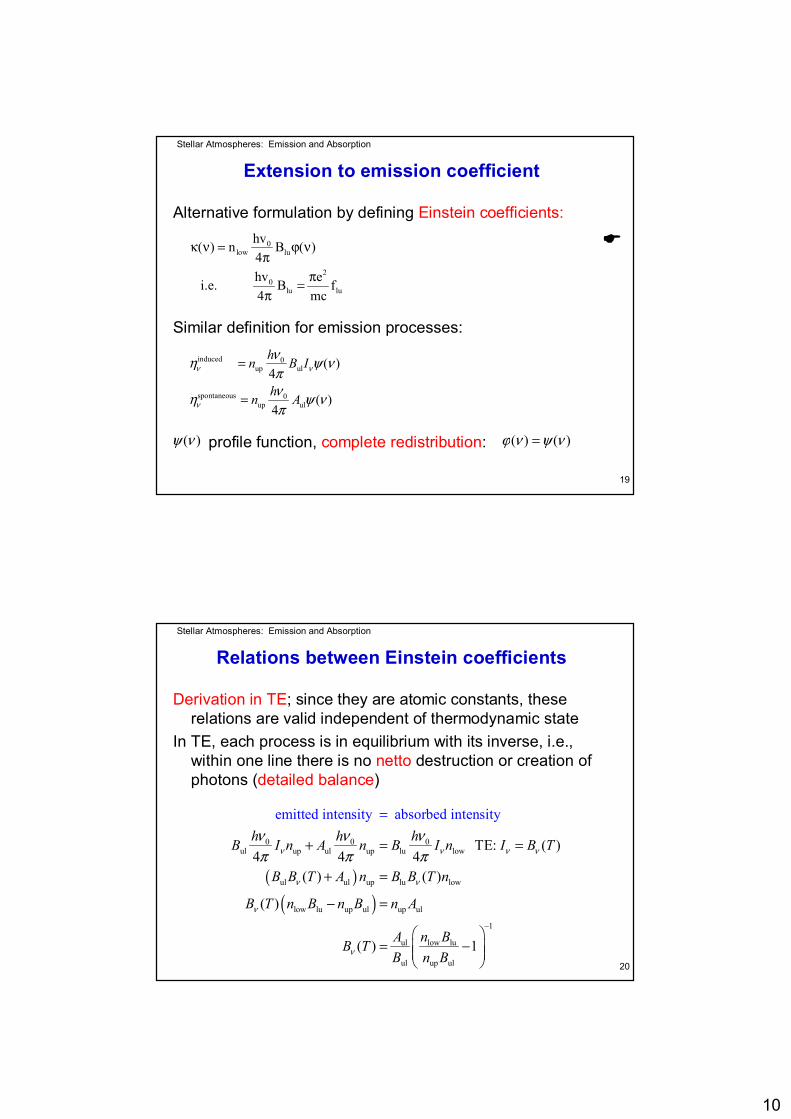
Extension to emission coefficient
Alternative formulation by defining Einstein coefficients:
Similar definition for emission processes:
profile function, complete redistribution:
induced 0up ul
spontaneous 0up ul
( )4
( )4
hn B I
hn A
ν ν
ν
νη ψ νπνη ψ νπ
=
=
0low lu
20
lu lu
hv( ) n B ( )4hv e i.e. B f 4 mc
κ ν = ϕ νπ
π=π
)(νψ )()( νψνϕ =
Stellar Atmospheres: Emission and Absorption
20
Relations between Einstein coefficients
Derivation in TE; since they are atomic constants, theserelations are valid independent of thermodynamic state
In TE, each process is in equilibrium with its inverse, i.e., within one line there is no netto destruction or creation of photons (detailed balance)
( )( )
0 0 0ul up ul up lu low
ul ul up lu low
low lu up ul up ul
1
ul low lu
ul up ul
TE: ( )4 4 4
( ) ( )
(
emitted intensity absorbed inte
)
nsity
( ) 1
h h hB I n A n B I n I B T
B B T A n B B T n
B T n B n B n A
A n BB TB n B
ν ν ν ν
ν ν
ν
ν
ν ν νπ π π
−
+ = =
+ =
− =
= −
=
11
Stellar Atmospheres: Emission and Absorption
21
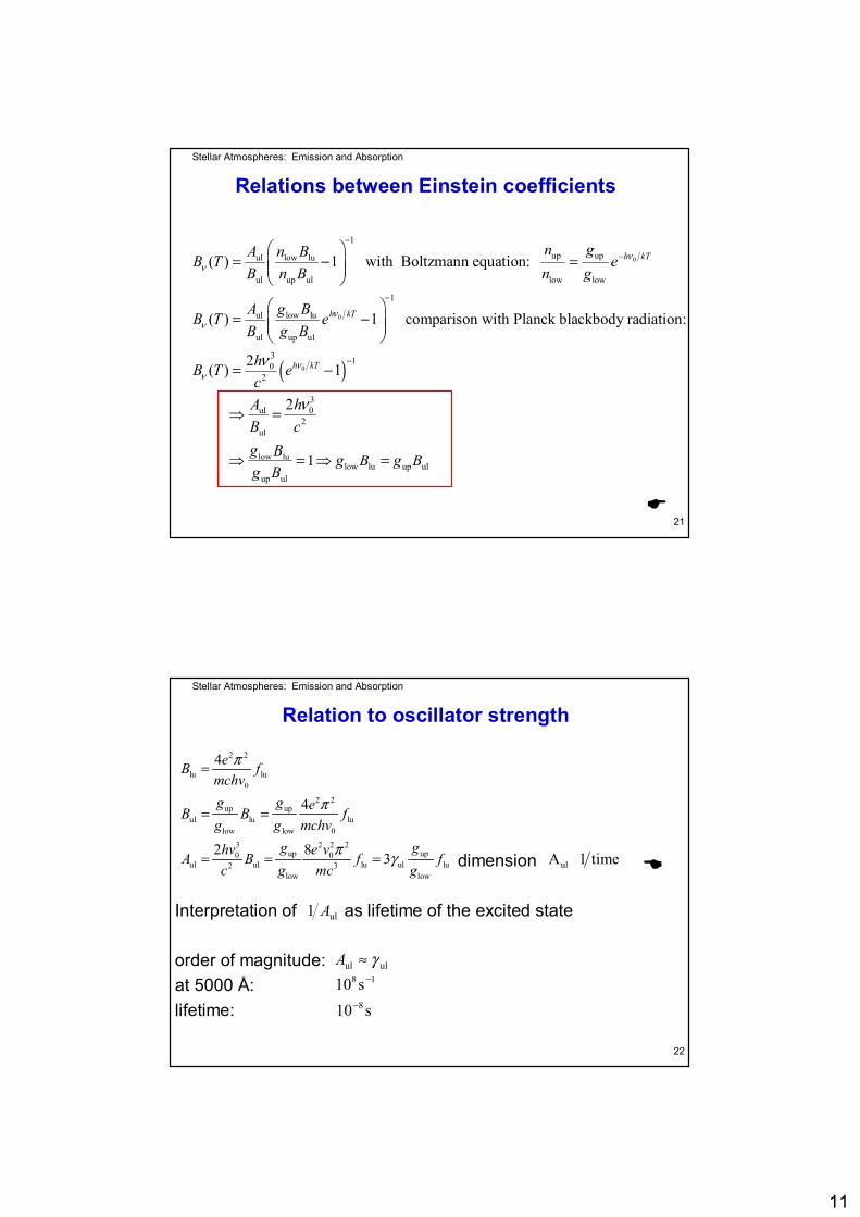
Relations between Einstein coefficients
( )
0
0
0
1
up upul low lu
ul up ul low low
1
ul low lu
ul up ul
3 102
( ) 1 with Boltzmann equation:
( ) 1 comparison with Planck blackbody radiation:
2( ) 1
h kT
h kT
h kT
n gA n BB T eB n B n g
A g BB T eB g B
hB T ec
νν
νν
νν
ν
−
−
−
−
= − =
= −
= −
⇒3
ul 02
ul
low lulow lu up ul
up ul
2
1
A hB cg B g B g Bg B
ν=
⇒ = ⇒ =
Stellar Atmospheres: Emission and Absorption
22
Relation to oscillator strength
dimension
Interpretation of as lifetime of the excited state
order of magnitude:at 5000 Å:lifetime:
2 2
lu lu0
2 2up up
ul lu lulow low 0
3 2 2 2up up0 0
ul ul lu ul lu2 3low low
4
4
2 8 3
eB fmchvg g eB B fg g mchv
g ghv e vA B f fc g mc g
π
π
π γ
=
= =
= = = ulA 1 time
ul1 A
ulul γ≈A18 s10 −
s10 8−
12
Stellar Atmospheres: Emission and Absorption
23
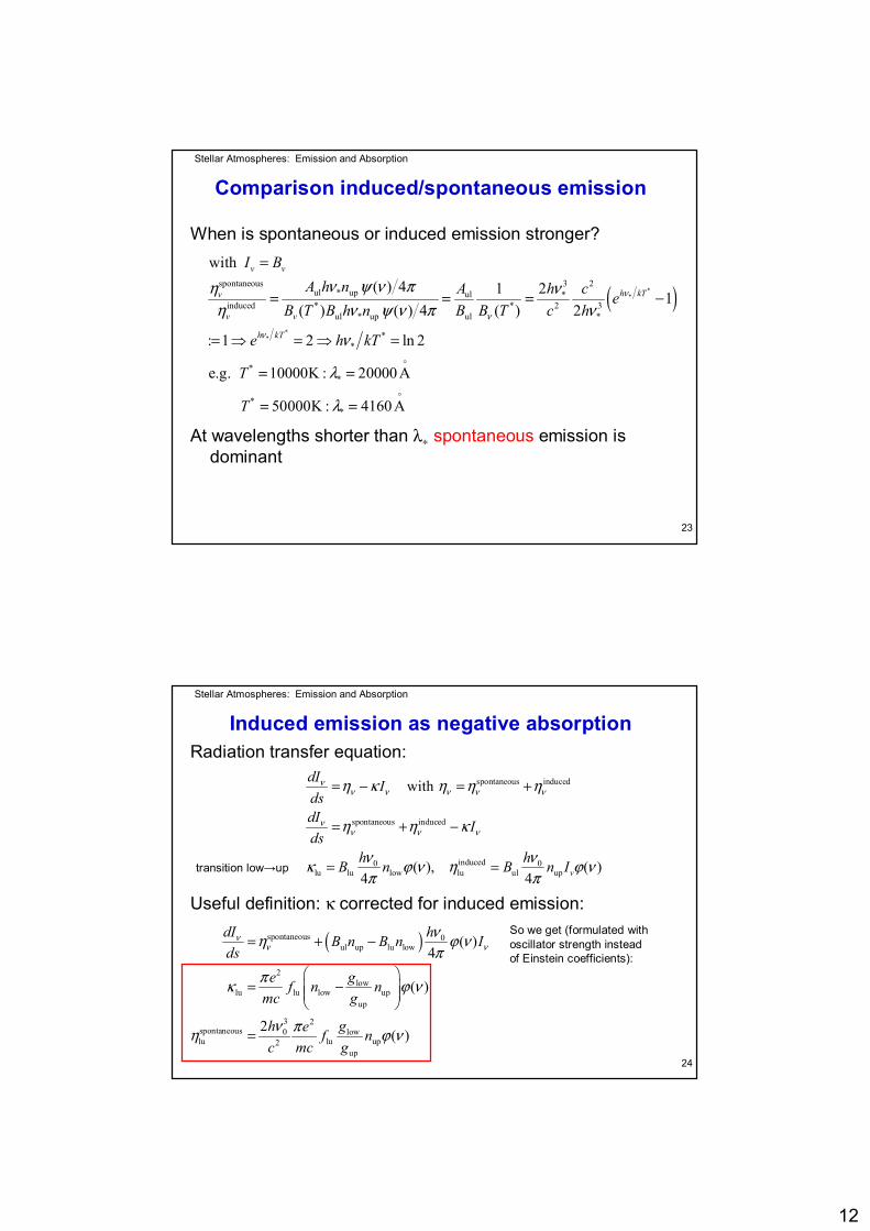
Comparison induced/spontaneous emission
When is spontaneous or induced emission stronger?
At wavelengths shorter than λ∗ spontaneous emission isdominant
( )**
**
spontaneous 3 2ul * up ul *
induced * * 2 3ul * up ul *
**
*
*
with ( ) 4 21 1
( ) ( ) 4 ( ) 2
: 1 2 ln 2
e.g. 10000K : 20000 A
50000K : 4160 A
v v
h kTv
v v
h kT
*
*
I BA h n A h c e
B T B h n B B T c h
e h kT
T
T
ν
ν
ν
ν ψ ν πη νη ν ψ ν π ν
ν
λ
λ
=
= = = −
= ⇒ = ⇒ =
= =
= =
o
o
Stellar Atmospheres: Emission and Absorption
24
Induced emission as negative absorptionRadiation transfer equation:
Useful definition: κ corrected for induced emission:
spontaneous induced
spontaneous induced
induced0 0lu lu low lu ul up
with
( ), ( )4 4
= − = +
= + −
= = v
dI IdsdI Ids
h hB n B n I
νν ν ν ν ν
νν ν ν
η κ η η η
η η κ
ν νκ ϕ ν η ϕ νπ π
( )spontaneous 0ul up lu low
2low
lu lu low upup
3 2spontaneous 0 lowlu lu up2
up
( ) 4
( )
2 ( )
dI hB n B n Ids
ge f n nmc g
h ge f nc mc g
νν ν
νη ϕ νπ
πκ ϕ ν
ν πη ϕ ν
= + −
= −
=
transition low→up
So we get (formulated withoscillator strength insteadof Einstein coefficients):
13
Stellar Atmospheres: Emission and Absorption
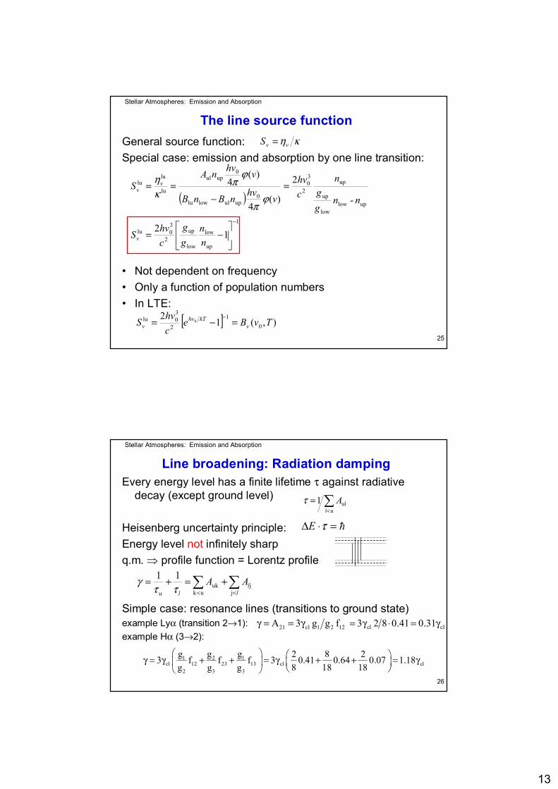
25
The line source functionGeneral source function:Special case: emission and absorption by one line transition:
• Not dependent on frequency• Only a function of population numbers• In LTE:
κηvvS =
( )1
up
low
low
up2
30lu
uplowlow
up
up2
30
0upullowlu
0upul
lu
lulu
12
-
2
)(4
)(4
−
−=
=−
==
nn
gg
chvS
nngg
nchv
vhvnBnB
vhvnAS
v
vv
ϕπ
ϕπ
κη
[ ] ),(120
1
2
30lu 0 TvBe
chvS v
kThvv =−=
−
Stellar Atmospheres: Emission and Absorption
26
Every energy level has a finite lifetime τ against radiative decay (except ground level)
Heisenberg uncertainty principle:Energy level not infinitely sharpq.m. ⇒ profile function = Lorentz profile
Simple case: resonance lines (transitions to ground state)example Lyα (transition 2→1):example Hα (3→2):
Line broadening: Radiation damping
∑<
=ul
ul1 Aτ
h=⋅∆ τE
∑∑<<
+=+=l
ll
AAj
juk
uku
11ττ
γ
21 cl 1 2 12A 3 g g fγ = = γ cl cl3 2 8 0.41 0.31= γ ⋅ = γ
1 2 1cl 12 23 13 cl cl
2 3 3
g g g 2 8 23 f f f 3 0.41 0.64 0.07 1.18g g g 8 18 18
γ = γ + + = γ + + = γ
14
Stellar Atmospheres: Emission and Absorption
27
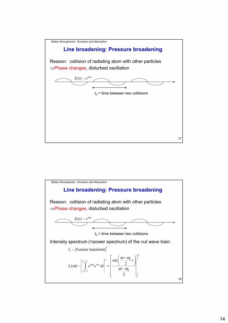
Line broadening: Pressure broadening
Reason: collision of radiating atom with other particles⇒Phase changes, disturbed oscillation
t0 = time between two collisions
0( ) ~ i tE t e ω
Stellar Atmospheres: Emission and Absorption
28
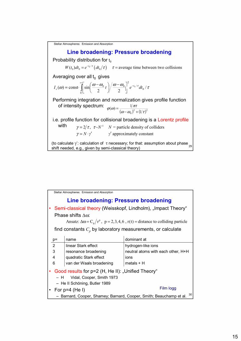
Line broadening: Pressure broadening
Reason: collision of radiating atom with other particles⇒Phase changes, disturbed oscillation
Intensity spectrum (=power spectrum) of the cut wave train:
t0 = time between two collisions
0
0
0
21
202/ 2
10/ 2
~ Fourier transform
sin2( ) ~
2−
− = −
∫t
i t i t
t
I
tI e e dtω ω
ω ω
ω ω ω
0( ) ~ i tE t e ω
15
Stellar Atmospheres: Emission and Absorption
29
Line broadening: Pressure broadeningProbability distribution for t0
Averaging over all t0 gives
Performing integration and normalization gives profile function of intensity spectrum:
i.e. profile function for collisional broadening is a Lorentz profile with
∫∞
−
−
−⋅=
00
/2
00 /22
sinconst)( 0 τωωωωω τ dtetI tv
( )0 /0 0 0( ) average time between two collisionstW t dt e dtτ τ τ−= =
( ) ( )220 11)(
τωωπτωϕ
+−=
12 , ~ = particle density of colliders approximately constant
-N NN γ γ
γ τ τγ
=′ ′= ⋅
(to calculate γ´: calculation of τ necessary; for that: assumption about phase shift needed, e.g., given by semi-classical theory)
Stellar Atmospheres: Emission and Absorption
30
Line broadening: Pressure broadening• Semi-classical theory (Weisskopf, Lindholm), „Impact Theory“
Phase shifts ∆ω:
find constants Cp by laboratory measurements, or calculate
• Good results for p=2 (H, He II): „Unified Theory“– H Vidal, Cooper, Smith 1973– He II Schöning, Butler 1989
• For p=4 (He I)– Barnard, Cooper, Shamey; Barnard, Cooper, Smith; Beauchamp et al.
ppAnsatz: C r , p 2,3, 4,6 , r(t) distance to colliding particle∆ω = = =
hydrogen-like ionsneutral atoms with each other, H+Hionsmetals + H
linear Stark effectresonance broadeningquadratic Stark effectvan der Waals broadening
2346
dominant atnamep=
Film logg
16
Stellar Atmospheres: Emission and Absorption
31
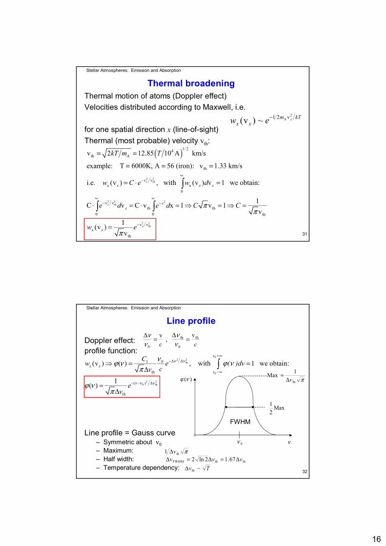
Thermal broadeningThermal motion of atoms (Doppler effect)Velocities distributed according to Maxwell, i.e.
for one spatial direction x (line-of-sight)Thermal (most probable) velocity vth:
kTmxx
xew2
A v21~)v( −
( )
2 2th
2 2 2th
1/ 24th A
th
v vx x
0
v vth th
0 0 th
x
v 2 12.85 10 A km/s
example: T 6000K, A 56 (iron): v 1.33 km/s
i.e. (v ) , with (v ) v 1 we obtain:
1C v C v x 1 v 1v
(v )
x
x
x x x
xx
x
kT m T
w C e w d
e d e d C C
w
ππ
∞−
∞ ∞− −
= =
= = =
= ⋅ =
⋅ = ⋅ = ⇒ = ⇒ =
=
∫
∫ ∫2 2
thv v
th
1v
xeπ
−
Stellar Atmospheres: Emission and Absorption
32
Line profile
Doppler effect:profile function:
Line profile = Gauss curve– Symmetric about ν0– Maximum:– Half width:– Temperature dependency:
ccth
0
th
0
v , v =∆=∆νν
νν
02 2
th
0
2 20 th
01
th
( )
th
(v ) ( ) , with 1 we obtain:
1( )
ν
x xν
Cw e ( )dνcν
eν
ν ν
ν ν ν
νϕ ν ϕ νπ
ϕ νπ
+∞−∆ ∆
−∞
− − ∆
⇒ = =∆
=∆
∫πth
1Maxv∆
=
Max21
0ν ν
)(νϕ
FWHM
πth1 v∆ththFWHM 67.12ln2 vvv ∆=∆=∆
Tv ~th∆
17
Stellar Atmospheres: Emission and Absorption
33
Examples
At λ0=5000Å:T=6000K, A=56 (Fe): ∆ λth=0.02ÅT=50000K, A=1 (H): ∆ λth=0.5ÅCompare with radiation damping: ∆ λFWHM=1.18 10-4Å
But: decline of Gauss profile in wings is much steeper thanfor Lorentz profile:
In the line wings the Lorentz profile is dominant
210 43th
2 6rad
Gauss (10 ) : e 10 Lorentz (1000 ) : 1 1000 10
− −
−
∆λ ≈≈
∆λ ≈
Stellar Atmospheres: Emission and Absorption
34
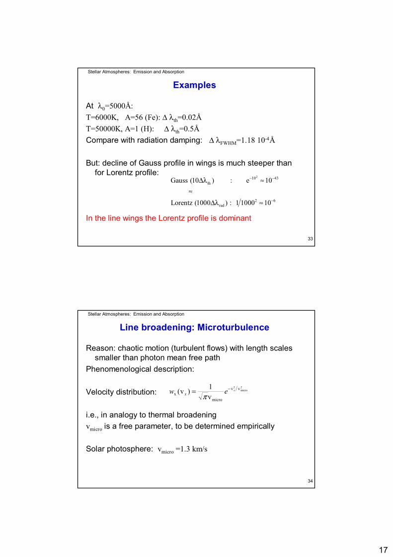
Line broadening: Microturbulence
Reason: chaotic motion (turbulent flows) with length scales smaller than photon mean free path
Phenomenological description:
Velocity distribution:
i.e., in analogy to thermal broadeningvmicro is a free parameter, to be determined empirically
Solar photosphere: vmicro =1.3 km/s
2micro
2 vv
microx v
1)v( xew x−=
π
18
Stellar Atmospheres: Emission and Absorption
35
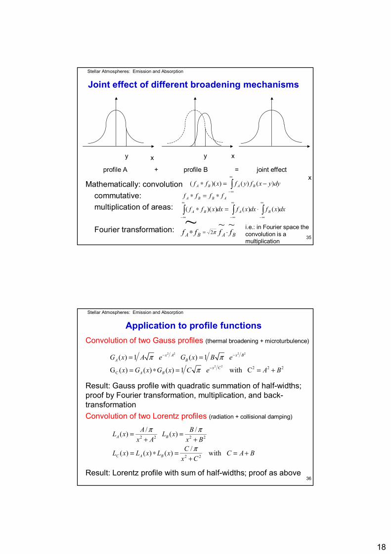
Joint effect of different broadening mechanisms
Mathematically: convolutioncommutative:multiplication of areas:
Fourier transformation:
y y xx
xprofile A + profile B = joint effect
dxxfdxxfdxxff BABA ∫∫∫∞
∞−
∞
∞−
∞
∞−
⋅=∗ )()())((
ABBA ffff ∗=∗∫∞
∞−
−=∗ dyyxfyfxff BABA )()())((
BABA ffff ⋅∗ =~~
2~
πi.e.: in Fourier space the convolution is a multiplication
Stellar Atmospheres: Emission and Absorption
36
Application to profile functionsConvolution of two Gauss profiles (thermal broadening + microturbulence)
Result: Gauss profile with quadratic summation of half-widths; proof by Fourier transformation, multiplication, and back-transformationConvolution of two Lorentz profiles (radiation + collisional damping)
Result: Lorentz profile with sum of half-widths; proof as above
2 2 2 2
2 2 2 2 2C
( ) 1 ( ) 1
G ( ) ( ) ( ) 1 with C
x A x BA B
x CA B
G x A e G x B e
x G x G x C e A B
π π
π
− −
−
= =
= ∗ = = +
2 2 2 2
2 2
/ /( ) ( )
/( ) ( ) ( ) with
A B
C A B
A BL x L xx A x B
CL x L x L x C A Bx C
π π
π
= =+ +
= ∗ = = ++
19
Stellar Atmospheres: Emission and Absorption
37
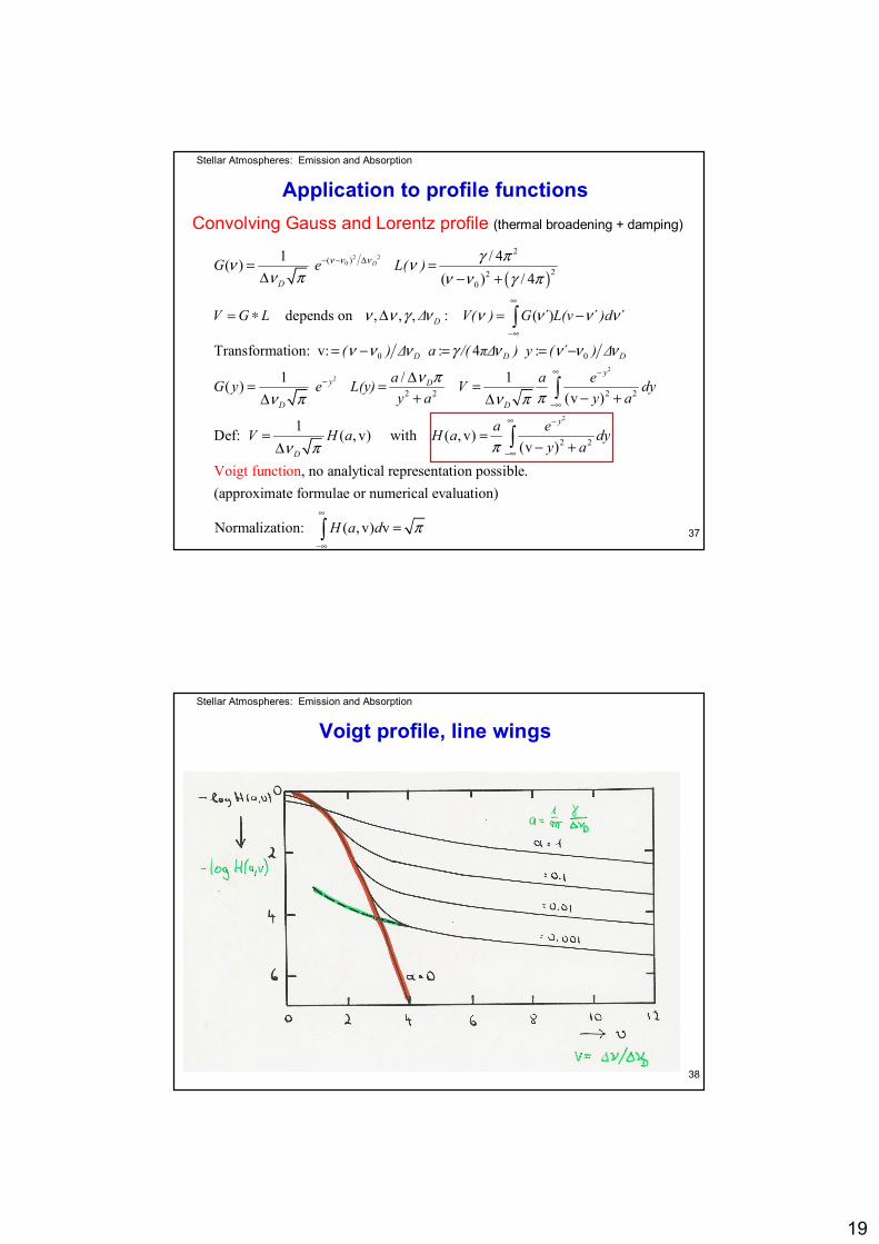
Application to profile functionsConvolving Gauss and Lorentz profile (thermal broadening + damping)
( )2 2
0
2
2( )
220
0 0
2
1 / 4( ) ( ) / 4
depends on , , : ( ´) ´ ´
Transformation: v: : 4 : ´
/1( )
− − ∆
∞
−∞
−
= =∆ − +
= ∗ , ∆ = −
= − = = −
∆= =+∆
∫
D
D
D
D D D
y D
D
G e L( )
V G L ∆ V( ) G L(v )d
( ) ∆ a /( π∆ ) y ( ) ∆
aG y e L(y)y
ν ν ν γ πν νν π ν ν γ π
ν ν γ ν ν ν ν ν
ν ν ν γ ν ν ν ν
ν πν π
2
2
2 2 2
2 2
Voigt fu
1 (v )
1Def: ( , v) with ( , v)(v )
, no analytical representation possible. (approximate formulae or numerical evaluation)
Norm
nc
a
o
l
ti n
∞ −
−∞
∞ −
−∞
=− +∆
= =− +∆
∫
∫
y
D
y
D
a eV dya y a
a eV H a H a dyy a
πν π
πν π
ization: ( , v) v∞
−∞
=∫ H a d π
Stellar Atmospheres: Emission and Absorption
38
Voigt profile, line wings
20
Stellar Atmospheres: Emission and Absorption
39
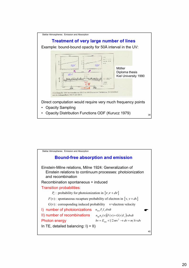
Treatment of very large number of linesExample: bound-bound opacity for 50Å interval in the UV:
Direct computation would require very much frequency points• Opacity Sampling• Opacity Distribution Functions ODF (Kurucz 1979)
MöllerDiploma thesisKiel University 1990
Stellar Atmospheres: Emission and Absorption
40
Bound-free absorption and emission
Einstein-Milne relations, Milne 1924: Generalization of Einstein relations to continuum processes: photoionizationand recombination
Recombination spontaneous + inducedTransition probabilities:
I) number of photoionizationsII) number of recombinationsPhoton energyIn TE, detailed balancing: I) = II)
[ ][ ]
: probability for photoionization in
(v) : spontaneous recapture probability of electron in v, v v(v) : corresponding induced probability v=electron velocity
P d
F dG
ν ν ν ν, +
+
[ ] dtdIGFnn v vv)v()v()v(eup +
dtdIPn vv νlow
v vv21 2ion dhmdvmEhv =→+=
21
Stellar Atmospheres: Emission and Absorption
41
Einstein-Milne relations[ ]
[ ]low up e
low up e
13 1low
2up e
3
2
low
up e
low up
(v) (v) (v) with
(v) (v) (v)
(v) 21 1(v) (v) (v)
(v) 2(v)
(v) (v)
f
v
v
h kTv
h kTv
n P I dvdt n n F G I h m dvdt I B
n P B n n F G B h m
n P mF hB eG n n hG c
F hG c
n P m en n hG
n n
ν ν ν ν
ν ν
νν
ν
ν
ν
−−
= + =
= +
= − = −
⇒ =
⇒ =
• ion
2
3/ 2uplow
2up e low
3/ 2v 2 2
e e e
2 2rom Saha equation:
(v) : Maxwell distribution: (v) v 4 v v2
E kT
m kT
gn mkT en n h g
mn n d n e dkT
π
ππ
−
−
=
• =
Stellar Atmospheres: Emission and Absorption
42
Einstein-Milne relations
Einstein-Milne relations, continuum analogs to Aji, Bji, Bij
2ion
3/ 2up 3/ 2
up
low
3
22
low2
up 23
lo
/ 2up
2e low
e
3/ 2v 2 2
e
w
(v)
2 4 v
8
(v)
4 v2
v(v
2 2
)
hv kT
m kTE kT
v
hv kT
v
n
mn ekT
P h eG m
h em
gh m m
nn
gmkT
m h ggP m
G h g
en h g
π
ππ
π
π
− −
=
=
=
=
22
Stellar Atmospheres: Emission and Absorption
43
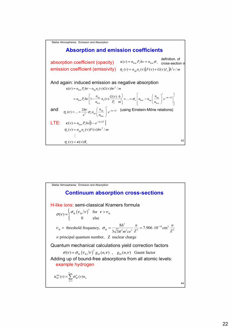
Absorption and emission coefficients
absorption coefficient (opacity)emission coefficient (emissivity)
And again: induced emission as negative absorption
and (using Einstein-Milne relations)
LTE:
vv nhvPnv σκ lowlow)( ==
[ ] mvhIGFnnv vv /)v()v()v()( 2eup +=η
2low up e
*up up /
low e low uplow low
( ) (v) (v) /
(v)1 (v) ... h kT
n P h n n G h m
n nG hn P h n n n en P m n
ν
νν ν
ν
κ ν ν ν
ν σ −
= −
= − = = −
[ ]
vv
v
kThvv
Bvv
mhFnnvehvPnv
)()(
/v)v()v()(
1)(2
eup
low
κη
ηκ
=
=
−= −
M
*up /
up3low
2( ) ...c
h kTnh n en
νν ν
νη ν σ − = =
definition. of cross-section σ
Stellar Atmospheres: Emission and Absorption
44
Continuum absorption cross-sections
H-like ions: semi-classical Kramers formula
Quantum mechanical calculations yield correction factors
Adding up of bound-free absorptions from all atomic levels: example hydrogen
( )3th th th
318 2
th th 2 22 2 2
for ( )0 else
8 threshold frequency, 7.906 10 cm3 3
principal quantum number, Z nuclear charge
h n nZ Zm ce
n
σ ν ν ν νσ ν
ν σπ
−
>=
= = = ⋅
( )3th th bf bf( ) ( , ) , ( , ) Gaunt factorg n g nσ ν σ ν ν ν ν=
∑=
=max
1bf
totbf )()(
n
nn
n nvv σκ
23
Stellar Atmospheres: Emission and Absorption
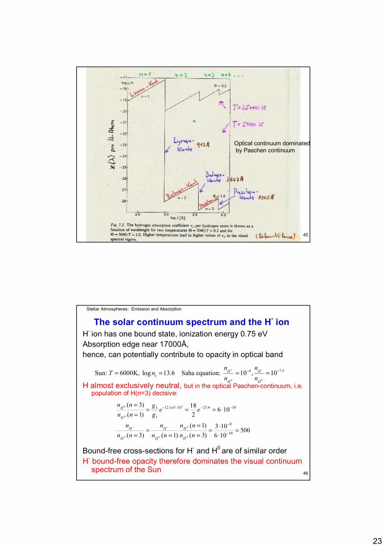
45
Continuum absorption cross-sections
Optical continuum dominatedby Paschen continuum
Stellar Atmospheres: Emission and Absorption
46
The solar continuum spectrum and the H- ionH- ion has one bound state, ionization energy 0.75 eVAbsorption edge near 17000Å,hence, can potentially contribute to opacity in optical band
H almost exclusively neutral, but in the optical Paschen-continuum, i.e. population of H(n=3) decisive:
Bound-free cross-sections for H- and H0 are of similar orderH- bound-free opacity therefore dominates the visual continuum
spectrum of the Sun
0 0
4 7.5eSun: 6000K, log 13.6 Saha equation: 10 , 10H H
H H
n nT n
n n+ −− −= = = =
500106103
)3()1(
)1()3(
1062
18)1()3(
10
8
104.23/eV1.12
1
3
0
0
00
0
0
=⋅⋅=
==
==
=
⋅=====
−
−
−−−
−−
nnnn
nnn
nnn
eegg
nnnn
H
H
H
H
H
H
kT
H
H
24
Stellar Atmospheres: Emission and Absorption
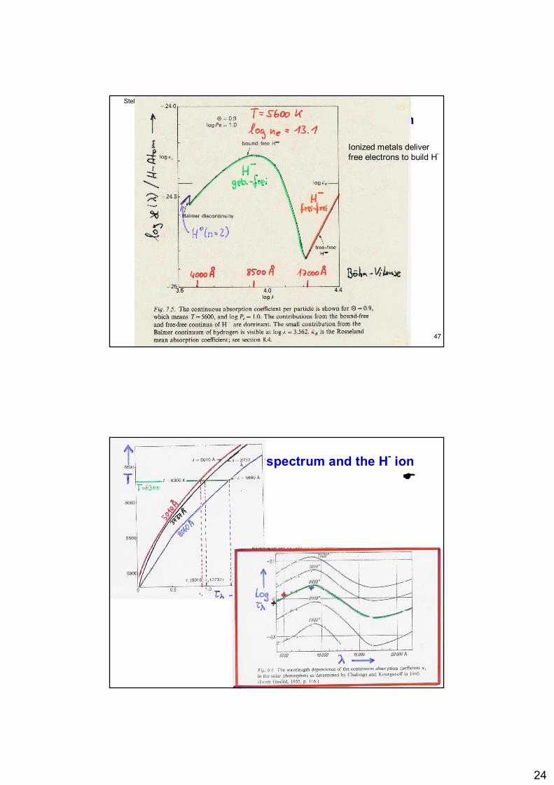
47
The solar continuum spectrum and the H- ion
Ionized metals deliver free electrons to build H-
Stellar Atmospheres: Emission and Absorption
48
The solar continuum spectrum and the H- ion
25
Stellar Atmospheres: Emission and Absorption
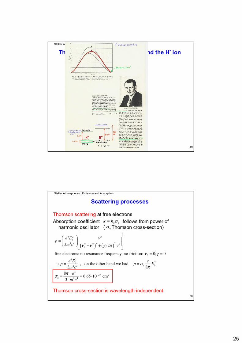
49
The solar continuum spectrum and the H- ion
Stellar Atmospheres: Emission and Absorption
50
Scattering processes
Thomson scattering at free electronsAbsorption coefficient follows from power of
harmonic oscillator ( Thomson cross-section)
Thomson cross-section is wavelength-independent
eeσκ n=eσ
( ) ( )
4 2 40
22 3 22 2 20
04 2
20e 02 3
425 2
e 2 4
3 2
free electrons: no resonance frequency, no friction: 0; 0
, on the other hand we had 3 8
8 6.65 10 cm3
e Epm c
e E cp p Em c
em c
νν ν γ π ν
ν γ
σπ
πσ −
= − + = =
→ = =
= = ⋅
26
Stellar Atmospheres: Emission and Absorption
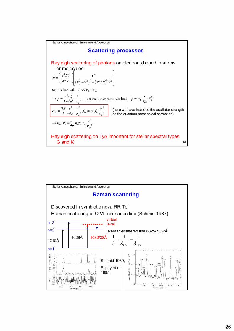
51
Scattering processes
Rayleigh scattering of photons on electrons bound in atomsor molecules
Rayleigh scattering on Lyα important for stellar spectral typesG and K
( ) ( )
4 2 40
22 3 22 2 20
04 2 4
20R 02 3 4
4 4 4
R lu e lu2 4 4 4
4
R e lu 4
3 2
semi-classical:
on the other hand we had 3 8
83
( )
lu
lu
lu lu
ll lu
e Epm c
e E cp p Em c
e f fm c
n f
νν ν γ π ν
ν ν νν σν π
π ν νσ σν ν
νκ ν σν
= − + << =
→ = =
= =
→ =∑
(here we have included the oscillator strengthas the quantum mechanical correction)
Stellar Atmospheres: Emission and Absorption
52
Raman scattering
Discovered in symbiotic nova RR TelRaman scattering of O VI resonance line (Schmid 1987)
n=1
n=2
n=3virtuallevel
1215Å1026Å 1032/38Å
Raman-scattered line 6825/7082Å
αLy OVI
111λλλ
−=
Schmid 1989,
Espey et al. 1995
27
Stellar Atmospheres: Emission and Absorption
53
Two-photon processes
Stellar Atmospheres: Emission and Absorption
54
Free-free absorption and emissionAssumption (also valid in non-LTE case):Electron velocity distribution in TE, i.e. Maxwell distribution
Free-free processes always in TESimilar to bound-free process we get:
generalized Kramers formula, with Gauntfaktor from q.m.• Free-free opacity important at higher energies, because
less and less bound-free processes present• Free-free opacity important at high temperatures
),()(/)()( ffffff TvBvvvS vvv == κη
( )ff h / kTff e k
2 2 6
ff ff3/ 2 3
( ) ( )n n 1 e
16 Z e( ) g (n, ,T)hc(2 T
1m)3 3
1
− νκ ν = σ ν −
πν
σ ν = ⋅ ⋅ νπ
1/ 2 3/ 2ffff bf bf~ T , but ~ T (Saha), therefore: / T − −σ σ κ κ
28
Stellar Atmospheres: Emission and Absorption
55
Computation of population numbers
General case, non-LTE:In LTE, just
In LTE completely given by:• Boltzmann equation (excitation within an ion)• Saha equation (ionization)
( , , )i i vn n T Iρ=( , )i in n Tρ=
Stellar Atmospheres: Emission and Absorption
56
Boltzmann equationDerivation in textbooks
Other formulations:• Related to ground state (E1=0)
• Related to total number density N of respective ion
( ) / statistical weight
excitation energy i jE E kT ii i
ij j
gn g e En g
− −=
kTEii iegg
nn /
11
−=
1 1
1 1 1
1
1
1
/
/partition function(
1
, with ( ) :)
−
−
= = =
= =→
∑
∑
∑ ∑ ∑ j
jE kTj
i i i i
jj j
i i
E kTj
n n n nn gnn n n n nn
g e
U Tn n g U g
nT
Ne
29
Stellar Atmospheres: Emission and Absorption
57
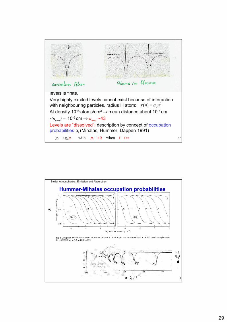
Divergence of partition function
e.g. hydrogen:
Normalization can be reached only if number of levels is finite.Very highly excited levels cannot exist because of interaction with neighbouring particles, radius H atom:At density 1015 atoms/cm3 → mean distance about 10-5 cmr(nmax) = 10-5 cm → nmax ~43Levels are “dissolved“; description by concept of occupation probabilities pi (Mihalas, Hummer, Däppen 1991)
i
2i i i Ion
E / kTi
g 2n g , E E
i.e. g ei i
i
lim lim
lim −
= → = ∞ =
= ∞→ ∞ → ∞
→ ∞
Nni
i =∑
20)( nanr =
with w0 hen → ∞→ →i i iig pg p i
Stellar Atmospheres: Emission and Absorption
58
Hummer-Mihalas occupation probabilities
30
Stellar Atmospheres: Emission and Absorption
59
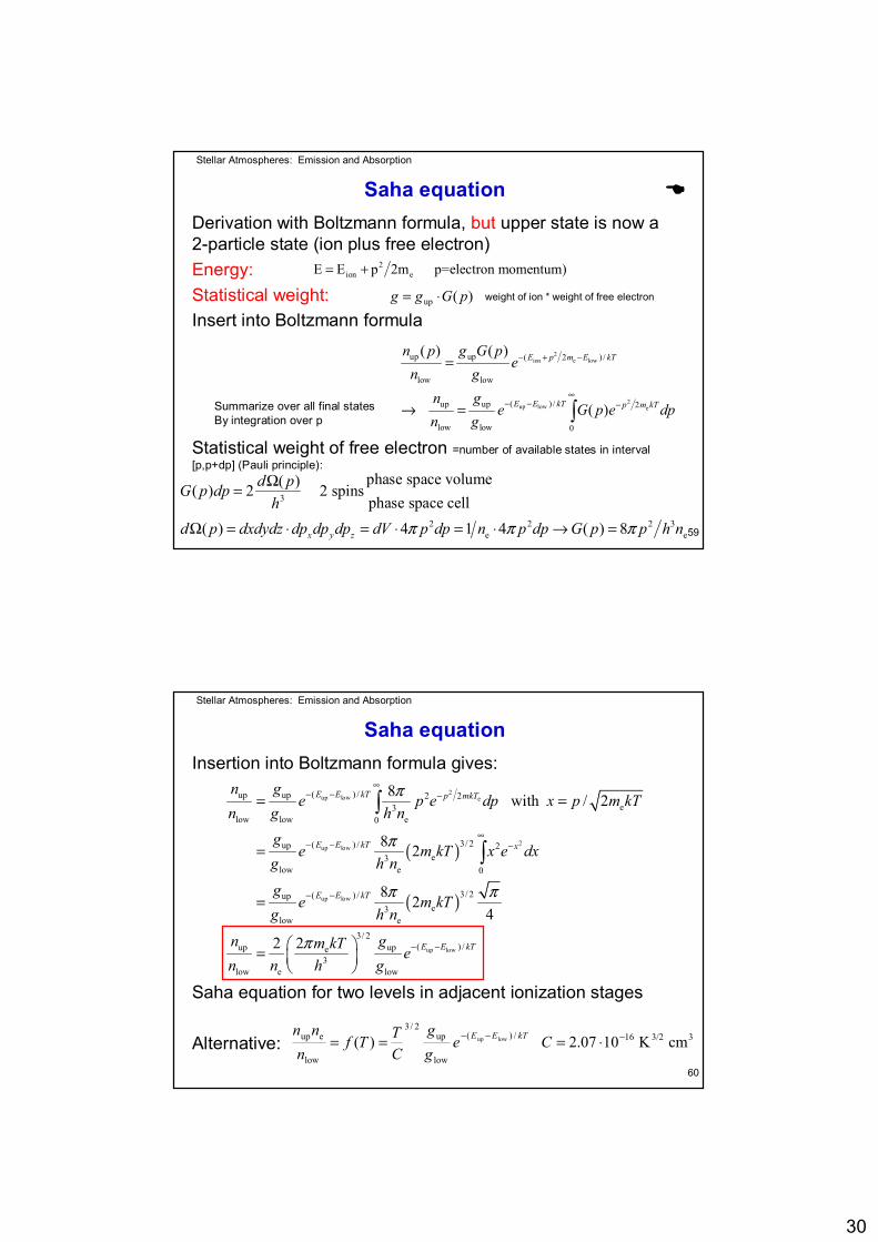
Saha equationDerivation with Boltzmann formula, but upper state is now a 2-particle state (ion plus free electron)Energy:Statistical weight:Insert into Boltzmann formula
Statistical weight of free electron =number of available states in interval[p,p+dp] (Pauli principle):
2ion eE E p 2m p=electron momentum)= +
)(up pGgg ⋅=
2ion e low
2up low e
up up ( 2 ) /
low low
( ) /up up 2
low low 0
( ) ( )
( )
E p m E kT
E E kT p m kT
n p g G pe
n gn g
e G p e dpn g
− + −
∞− − −
=
→ = ∫
3
2 2 2 3e e
phase space volume( )( ) 2 2 spinsphase space cell
( ) 4 1 4 ( ) 8x y z
d pG p dph
d p dxdydz dp dp dp dV p dp n p dp G p p h nπ π π
Ω=
Ω = ⋅ = ⋅ = ⋅ → =
weight of ion * weight of free electron
Summarize over all final statesBy integration over p
Stellar Atmospheres: Emission and Absorption
60
Saha equationInsertion into Boltzmann formula gives:
Saha equation for two levels in adjacent ionization stages
Alternative:
( )
( )
2up low e
2up low
up low
up
( ) /up up 22e3
low low e0
3/ 2( ) /up 2e3
low e 0
3/ 2( ) /upe3
low e
3/ 2(up upe
3low e low
8 with / 2
8 2
8 24
22
E E kT p mkT
E E kT x
E E kT
E
n ge p e dp x p m kT
n g h ng
e m kT x e dxg h n
ge m kT
g h n
n gm kT en n h g
π
π
π π
π
∞− − −
∞− − −
− −
−
= =
=
=
=
∫
∫
low ) /E kT−
33/216/)(
low
up2/3
low
eup cm K 1007.2 )( lowup −−− ⋅=== Cegg
CTTf
nnn kTEE
31
Stellar Atmospheres: Emission and Absorption
61
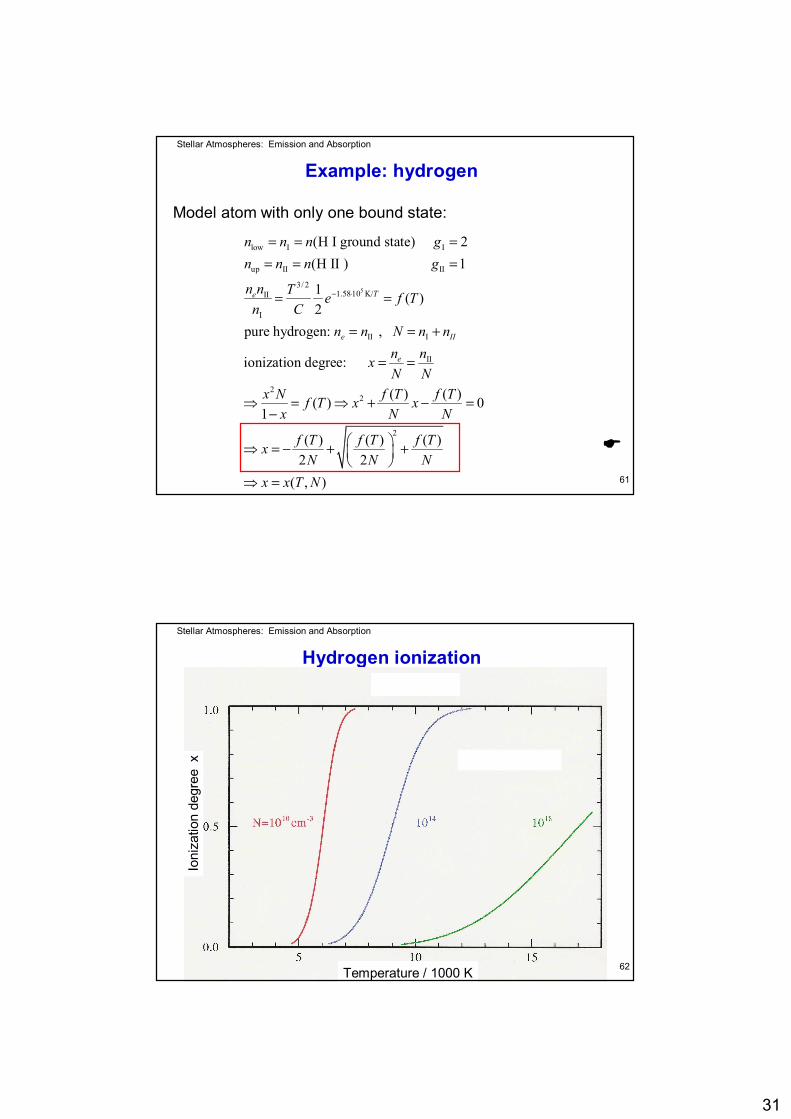
Example: hydrogen
Model atom with only one bound state:
5
low I I
up II II
3/ 21.5810 K/II
I
II I
II
22
(H I ground state) 2(H II ) 1
1 ( )2
pure hydrogen: ,
ionization degree:
(( )1
Te
e II
e
n n n gn n n g
n n T e f Tn C
n n N n nn n xN N
x N f Tf T xx
− ⋅
= = == = =
= =
= = +
= =
⇒ = ⇒ +−
2
) ( ) 0
( ) ( ) ( )2 2
( , )
f TxN N
f T f T f TxN N N
x x T N
− =
⇒ = − + +
⇒ =
Stellar Atmospheres: Emission and Absorption
62
Hydrogen ionization
Ioni
zatio
n de
gree
x
Temperature / 1000 K
32
Stellar Atmospheres: Emission and Absorption
63
More complex model atoms
j=1,...,J ionization stagesi=1,...,I(j) levels per ionization stage jSaha equation for ground states of ionization stages j and j+1:
With Boltzmann formula we get occupation number of i-th level:
kTEegg
kTmhnnn /
11j
1j2/3
e
3
e1j1j1
jIon
221
++
=
π
kTEE
kTEkTE
eTCnngg
n
egg
TCnnegg
nnn
n
/)(2/31e1j1
11j
ijij
/
11j
1j2/31e1j1
/
1j
ij1j
1j
ijij
ji
jIon
jIon
ji
−−+
+
+
−+
−
=⇒
==
Stellar Atmospheres: Emission and Absorption
64
More complex model atoms
Related to total number of particles in ionization stage j+1
Nj/Nj+1
kTEEkTEE eTCnNUg
neTCnNUg
gg
n
NUg
nUg
Nn
Ug
nn
Nn
/)(2/31e1j
1j
ijij
/)(2/31e1j
1j
11j
11j
ijij
1j1j
11j11j
1j
11j
1j
11j
1j
11j
11j
1ij
1j
1ij
ji
jIon
ji
jIon
1 1i
−−+
+
−−+
+
+
+
++
++
+
+
+
+
+
+
+
+
+
+
=⇒=⇒
=→⋅== =
)(je/2/3
1e1j
j
1j
j
j/2/3
1e1j
1j
i
/ij
/2/31e
1j
1j
i
/)(2/31e1j
1j
ij
iijj
jIon
jIon
ji
jIon
ji
jIon
TneTCnUU
NN
UeTCnUN
egeTCnUN
eTCnNUg
nN
kTE
kTEkTEkTE
kTEE
Φ==
==
==
−
++
−
+
+−−
+
+
−−+
+
∑
∑∑
33
Stellar Atmospheres: Emission and Absorption
65
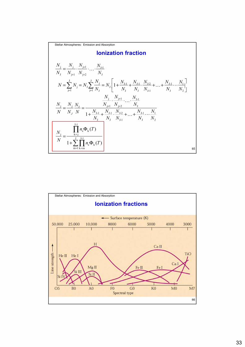
Ionization fraction
j j j 1 J-1
J j 1 j 2 J
J Jj J-1 J-1 J-2 J-1 1
j J Jj 1 j 1 J J J J-1 J 2
j j 1 J-1
j j j 1 j 2 JJ
J-1 J-1 J-2 J-1 1
J J J-1 J 2J-1
e kj k j
e kk
1
1
( )
1 ( )
J
N N N NN N N N
N N N N N NN N N NN N N N N N
N N NN N N N NN
N N N N NN N NN N N N N
n TNN n T
+
+ +
= =
+
+ +
=
=
= ⋅ ⋅ ⋅
= = = + + ⋅ + +
⋅ ⋅ ⋅= =
+ + ⋅ + +
Φ=
+ Φ
∑ ∑
∏
K
K L
K
K L
J-1J
m 1 m=∑∏
Stellar Atmospheres: Emission and Absorption
66
Ionization fractions
34
Stellar Atmospheres: Emission and Absorption
67
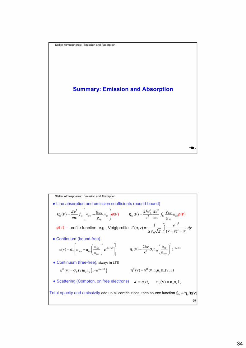
Summary: Emission and Absorption
Stellar Atmospheres: Emission and Absorption
68
Line absorption and emission coefficients (bound-bound)32 2
low 0 lowlu lu low up lu lu up2
up up
( ) 2
( ) ( ) ( )
= − =
g h ge ef n n f nmc g c mc g
νπ πκ ν η νϕ ν ϕ ν
profile function, e.g., Voigtprofile( ) =ϕ ν2
2 21( , v)
(v )
∞ −
−∞
=− +∆ ∫
y
D
eV a dyy aν π
Continuum (bound-free)*
up h / kTlow up
low
n(v) n n e
n− ν
ν
κ = σ −
*up h /kT
up3low
n2h( ) n ec n
− νν ν
νη ν = σ
Continuum (free-free), always in LTE
( )ff -h / kTff e k( ) ( )n n 1-e νκ ν = σ ν ff ff
e k( ) ( )n n B ( ,T)νη ν = κ ν ν
eeσκ n= Scattering (Compton, on free electrons)e en Jν νη (ν) = σ
Total opacity and emissivity add up all contributions, then source function S ( )ν ν= η /κ ν
35
Stellar Atmospheres: Emission and Absorption
69
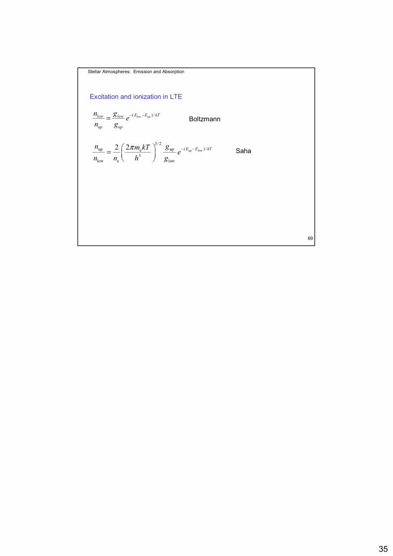
Excitation and ionization in LTE
( ) /− −= low upE E kTlow low
up up
n g en g
up low
3 /2( ) /up upe
3low e low
22 − − =
E E kTn gm kT en n h g
π
Boltzmann
Saha