1

1

Electrostatics in material

z η0 ˆP P z=

θ

R

Q

ε

r

0εε

aboveEbelowE

Z

sε

0εq

bσα

z η

ε0εHF

Fd

x− xx

R

z

ε 0 ˆE z

0σ >b

σf

σ− f

d

VtopD

bottomD

εE

0σ <b

I

Bound charges

Displacement field

Dielectric boundary conditions

Dielectric Forces

Stored energy in a dielectric

Laplacean methods and dielectrics

Image methods Separation of variables

From Physics 212, one might get the impression that going from electrostatics in vacuum to electrostatics in a material is equivalent to replacing epsilon_0 to epsilon > epsilon_0. This is more-or-less true for some dielectric materials such as Class A dielectrics but other types of materials exist. For example, there are permanent electrets which are analogous to permanent magnets. Here the electric field is produced by “bound” charges created by a permanently “frozen-in” polarizability. The polarizability is the electric dipole moment per unit volume that is often induced in the material by an external electric field. We will introduce the displacement field (or D-field) which obeys a Gauss’s Law that only depends on free charges. Free charges are the charges controllable by batteries, currents and the like. To a large extent one cannot totally control bound charges. We discuss the boundary conditions that E-fields and D-fields obey across a dielectric boundary. We turn next to a discussion of Laplace’s Equation in the presence of dielectrics. We give a “method-of-images” solution for a charge above a dielectric surface and a separation of variable solution for a dielectric sphere placed in a uniform electric field. These examples make extensive use of the dielectric boundary conditions. We turn next to a discussion of energy storage in the presence of dielectrics. There are some interesting new issues that arise concerned with whether or not one includes or excludes the energy stored by the bound charges. We next consider the forces that act on a dielectric that – for example– tend to pull the dielectric into the plates of a capacitor. We will conclude on a more detailed model for the dielectric constants of a material that can be used for material composites called the Clausius-Mossotti Equation.

2

2

Matter response to E: Induced dipole moment

200 2102

ψ 2

+=

+ +

−−−

+

+ +−−

−

−−

−−−

−

+ +

e- “falls” in direction of applied force – against E

2 0

00 0

0 00

200 210 with z 3

233 3 tanh

3 3as kT 3 , tanh

and and ||

a

ea Ea E p eakT

ea E ea Eea EekT kT

p E p E

ψ±

= =

⎛ ⎞ΔΕ = ± → → ⎜ ⎟⎝ ⎠

⎛ ⎞ ⎛ ⎞→⎜ ⎟ ⎜ ⎟⎝ ⎠ ⎝ ⎠

∝

∓

200 210+

1ψ 21±

200 210−

03exp

ea E

kT

⎛ ⎞⎜ ⎟⎜ ⎟⎝ ⎠

03exp

ea E

kT

⎛ ⎞−⎜ ⎟⎜ ⎟⎝ ⎠

Stark effect

probabilities

p< >

1/T

Massively oversimplified

Here is an old slide from my Quantum mechanic course that shows how a hydrogen atom would respond to an external electric field and create a net dipole moment. The basic idea is initially degenerate states – say the initially degenerate 200 and 210 states in hydrogen have no dipole moment since they have no preferred direction. However once an external field is applied they can form a linear combination of these two states which allows the electron to lower its energy by “falling” into the electric force and creating an asymmetric wave function. That has a dipole moment. In this case the dipole moment is parallel to the external electric field. The other combination has the electron cloud on the other side of the hydrogen proton which produces an anti-parallel dipole moment and thus lies higher in energy since U = - p dot E. Of course we won’t always find the electron in the lower state at finite temperatures because of thermal fluctuations. We thus expect the polarization to vanish at low 1/T which is high temperatures.

3

3

Polarization per volumeWhen an E-field is applied to matter it polarizesthe molecules in the matter in a way parameterized

by P(r) where P is the dipole moment per unit volume We will show that P creates "bound" charg

0

es in

in a Often P E or

for linear dielectric we will show 1which is familiar from capacitors in Physics 212. The familiar linear, uniform Phys 212 dielec

"dielectri

tric is

c".

( )e

eP E

ε ε

χ

χ

ε

0

=∝

= +

a dielectric but other possibilities exist. In crystals can be a non-diag 3 3 matrix

P is not parallel to E

One even has permanent P such as

"Class A"

in

e

xx xy xz

e yx yy yz

zx zy zz

χ

χ χ χ

χ χ χ χ

χ χ χ

×

⎛ ⎞⎜ ⎟

= →⎜ ⎟⎜ ⎟⎝ ⎠

a bar which is analogy to barelectre magt net.

20

We will show two amazing analogies:

Recall for dipole 4

for dielectr

Bo

i

und charges and Polarization P

cs d

;

ˆ( )

( ') ( ') '

ˆ ˆf b

f b

r pV rr

dp

E

r r

E

P

P

P

rπ

ε ρ ρ

σ ε η σ

ετ

η0

0

∇ = ⇔ −∇ =

=

=

= −

⇔ =

i i

i

i

i

3 30

0

1 or d . Using 4

1 1We have d4

'( ')( ) ' '

( ) ( ') ' '

r

P rV r

V r P r

τπε

τπε

=

⎧ ⎫= ∇ =∫ ⎨ ⎬⎩ ⎭

⎡ ⎤= ∇∫ ⎢ ⎥⎣ ⎦

r

rrr

r

rr

i

i

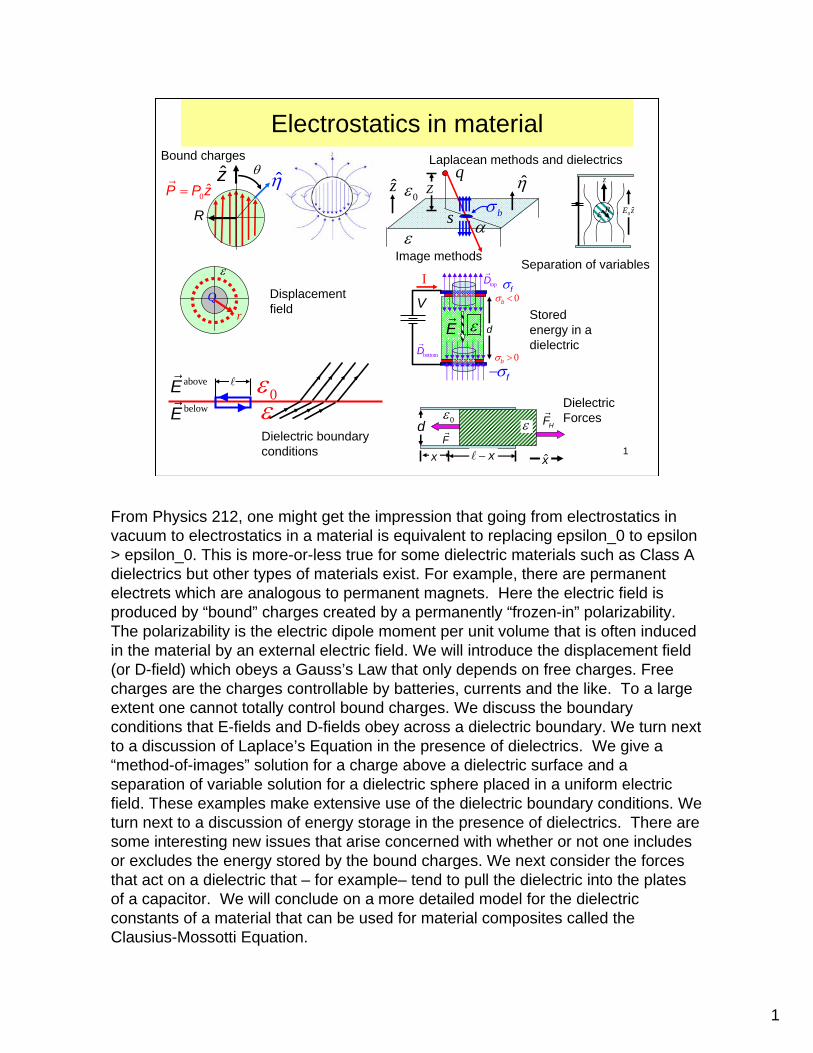
An electrical field applied to matter will typically polarize the atoms or molecules as shown before. This polarization is parameterized by a polarization density P(r) giving the dipole moment per unit volume which is a function of position in the matter. Usually we will consider linear dielectric where the polarization density is proportional to the E-field with a proportionality constant given by the susceptibility chi times the constant epsilon. In these cases P is parallel to E. It is also possible that P is not parallel to E – in which case the susceptibility is represented by a 3 by 3 matrix. There are even cases where there can be a permanent P in the absence of a E-field. The polarization density can create a bound charge surface density and volume density. This is the key result for this chapter. Our first step is to use the expression for the potential of a dipole developed in the Laplace chapter in terms of a volume integral over a polarization density. We our dipole potential is an approximate expression with corrections which are proportional to powers in (r’/r) where r’ is the size of the molecular electron cloud (~10^-8 – 10^-7 cm) and r is is the position of the observer relative to the molecule (~ 1 cm). Hence our approximation should be very accurate. We next exploit a neat mathematical identity that the gradient of 1/r is essentially 1/r^2 times the r unit vector. This same identity can be used to show that the E-field which goes as 1/r^2 is the -gradient of the Coulomb potential that goes as 1/r. The missing minus sign comes from nabla’ = - nabla. This allows us to write the V(r) in a way that is suitable for integration by parts.

4

4

Bound and Free charges

0

1 1 d4

We next use this theorem from Potential Chp

1with and

1 4

( ) ( ') ' '

( ) ( ) ( ) ( )

( )

'( ) ' ( ) '' '

S V V

S V

V r P r

f r r da f r d r f d

P f r

PP r da V r dr r r r

V

τπε

τ τ

πε τ0

⎡ ⎤= ∇∫ ⎢ ⎥⎣ ⎦

Α = ∇ Α + Α ∇∫ ∫ ∫

Α → =

∇= +∫ ∫

− −

r

r

i

i i i

ii

1 1 4

'( ) ( ) ' 'S V

Pr P r da dτπε0

⎡ ⎤∇= −∫ ∫⎢ ⎥

⎣ ⎦rrii

We can write this as1

41

4

where and

( ) '

( ') '

ˆ

b

S

b

V

b b

V r da

r d

P P

σπερ

τπε

σ η ρ

0

0

= ∫

+ ∫

= = −∇

r

ri i

Bound charges are real charges

totb

We show total bound charge is zero using divergence thm

Q 0

ˆ

bV V S

bS S S

b bS V

d Pd P da

da P da P da

da d

ρ τ τ

σ η

σ ρ τ

= − ∇ = −∫ ∫ ∫

= =∫ ∫ ∫

⇒ = + =∫ ∫

i i

i i

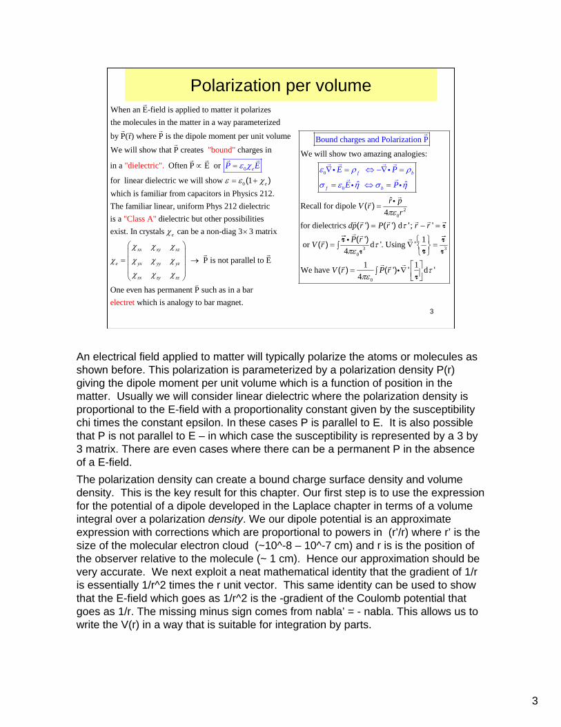
We next rearrange our V(r) expression, which is the potential contribution due to the molecules of the material, using an integration by parts expression first introduced in the Potential chapter. We are not writing the full potential – only the part due to the induced dipole moment in the material. Essentially the integration allow us to move the del operator from the 1/r term to the Polarization density. We are left with an expression for the V(r) consisting of a surface integral over P and a volume integral over the divergence of P. In both cases we have the 1/r factor that usually multiples charges in potentials. The surface integral suggests that P creates a surface charge density of bound charge, and the volume integral suggests that the divergence of P represents a bound charge density -- in much the same way as the divergence of E is proportional to the free charge density. In the surface integral, we assign the area vector to be in the direction eta which is “out” of the dielectric. Although the bound surface charge and bound charge volume density are first revealed through some slick mathematical manipulations – they definitely represent real charges that are bound in the dielectric. As such they will contribute to the E-field. Griffiths discusses some models for the “bound” charge. We can easily show that the total bound charge is zero using the divergence theorem. The bound charge volume density is negative of the divergence of the polarization density. The divergence theorem says this is equal to the negative of the surface integral over the surface that bounds the dielectric. The integral of the surface density is the area integral constructed of the dot product of the polarization vector and area vector. The surface bound charge integral exactly cancels the volume bound charge integral so there is no net bound charge when one considers the surface density and volume density over a full dielectric region.

5

5

Bound charge reduces field from free charges

;

; 1

Thus with 11

ˆ ;

ˆˆ ˆ &

ˆ ˆ(

ˆ ˆ ˆ; (

(

rb b b

fbb f

f ff b

f f f

P E P E E

E xE x x E E

x xE E E E E

x x xE E

ε χ σ η σ ε χ σ ε χ

ε χ σσχ

ε ε εσ σ

χ χε ε

σ σ σε ε χ

ε χ ε ε

0 0 0

0

0 0 0

0 0

00 0

= = → = − = +

+= − = − = − =

⇒ = + = − + ) =

= < = = + )+ )

i

+++++

−−−−−

−−−−−

P+++++

ηη /b bE σ ε0=

0/f fE σ ε=

x

phys 212 Griffiths

0

1 1 In capacitors:

;

fr

air

QEA

AQd Q AV E C CA V d d

σε κ ε χε ε ε

εε κε

0

= = = + > = =

Δ = × = = = = >Δ

+−E

+−E

+−E

+−E

+−E

+++++

−−−−−

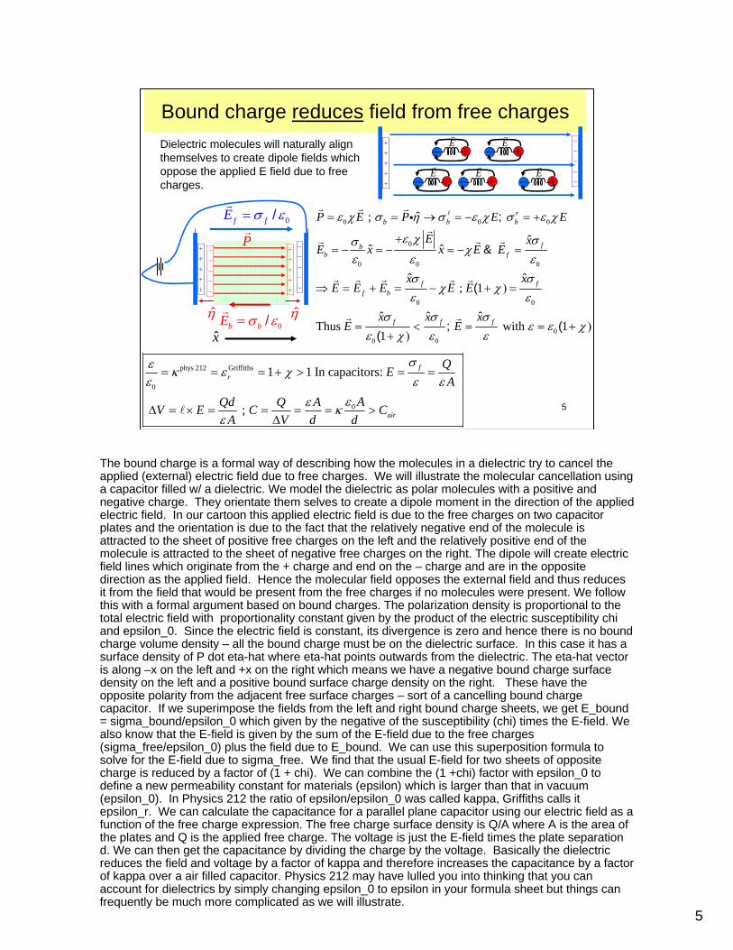
Dielectric molecules will naturally align themselves to create dipole fields which oppose the applied E field due to free charges.

The bound charge is a formal way of describing how the molecules in a dielectric try to cancel the applied (external) electric field due to free charges. We will illustrate the molecular cancellation using a capacitor filled w/ a dielectric. We model the dielectric as polar molecules with a positive and negative charge. They orientate them selves to create a dipole moment in the direction of the applied electric field. In our cartoon this applied electric field is due to the free charges on two capacitor plates and the orientation is due to the fact that the relatively negative end of the molecule is attracted to the sheet of positive free charges on the left and the relatively positive end of the molecule is attracted to the sheet of negative free charges on the right. The dipole will create electric field lines which originate from the + charge and end on the – charge and are in the opposite direction as the applied field. Hence the molecular field opposes the external field and thus reduces it from the field that would be present from the free charges if no molecules were present. We follow this with a formal argument based on bound charges. The polarization density is proportional to the total electric field with proportionality constant given by the product of the electric susceptibility chi and epsilon_0. Since the electric field is constant, its divergence is zero and hence there is no bound charge volume density – all the bound charge must be on the dielectric surface. In this case it has a surface density of P dot eta-hat where eta-hat points outwards from the dielectric. The eta-hat vector is along –x on the left and +x on the right which means we have a negative bound charge surface density on the left and a positive bound surface charge density on the right. These have the opposite polarity from the adjacent free surface charges – sort of a cancelling bound charge capacitor. If we superimpose the fields from the left and right bound charge sheets, we get E_bound= sigma_bound/epsilon_0 which given by the negative of the susceptibility (chi) times the E-field. We also know that the E-field is given by the sum of the E-field due to the free charges (sigma_free/epsilon_0) plus the field due to E_bound. We can use this superposition formula to solve for the E-field due to sigma_free. We find that the usual E-field for two sheets of opposite charge is reduced by a factor of (1 + chi). We can combine the (1 +chi) factor with epsilon_0 to define a new permeability constant for materials (epsilon) which is larger than that in vacuum (epsilon_0). In Physics 212 the ratio of epsilon/epsilon_0 was called kappa, Griffiths calls it epsilon_r. We can calculate the capacitance for a parallel plane capacitor using our electric field as a function of the free charge expression. The free charge surface density is Q/A where A is the area of the plates and Q is the applied free charge. The voltage is just the E-field times the plate separation d. We can then get the capacitance by dividing the charge by the voltage. Basically the dielectric reduces the field and voltage by a factor of kappa and therefore increases the capacitance by a factor of kappa over a air filled capacitor. Physics 212 may have lulled you into thinking that you can account for dielectrics by simply changing epsilon_0 to epsilon in your formula sheet but things can frequently be much more complicated as we will illustrate.

6

6

Bound charge shields free charge

0

We can view as layer of shielding 1

each so or (either plate)1

We can easily show this works even for within dielectric.

ˆ ˆ(

(

-

f fb

ff b f

f

b

fb

x xE

P E P

σ σσ

ε χ ε κ

σσ σ σ

χ

ρ

ε χ ρ ε

χσσ

χ

χ

0 0

0

= −1+

= =+ )

+ =+ )

= → ∇ = = ∇i i ( )

( )

(If

f

f b

ffbb f b b

E χ ρ ρ χ

ρρ

χρρρ ρ

χχ ρ ρ

χ

= + ∇ = 0)

= − + = − →→ + =1+ 1+

−−−−−

+++++

⊗

1(

fb f

ρρ ρ

χ+ =

+ )

fq

1(

fb f

σσ σ

χ+ =

+ ) ( )

2

22

2 2

and again or 1 1

4 4

ˆ ˆ

ˆ( ) ˆ

f bb

f bb b b f b

f f fb b f

f b f

Q QE r P E r P

RQ Q

Q R Q QR

Q Q QQ Q Q

Q Q QrE r R rr r

ε χ σπε

σ ε χ πε σ χπε

χχ χ κ

πε κ πε

00

00

0 0

+= → = → = −

4

+= − → = 4 = − +

4

−= + = =

+ ++

> = =

i

fQ

χ

rR−

−

−

−−−

bQ

A mistaken impression is that all that dielectrics do is add a factor of 1/κ

Charged sphere in dielectric

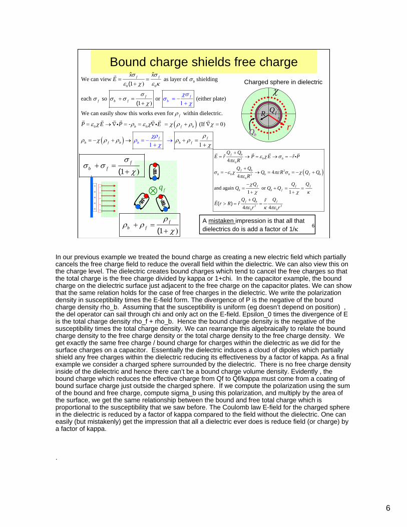
In our previous example we treated the bound charge as creating a new electric field which partially cancels the free charge field to reduce the overall field within the dielectric. We can also view this on the charge level. The dielectric creates bound charges which tend to cancel the free charges so that the total charge is the free charge divided by kappa or 1+chi. In the capacitor example, the bound charge on the dielectric surface just adjacent to the free charge on the capacitor plates. We can show that the same relation holds for the case of free charges in the dielectric. We write the polarization density in susceptibility times the E-field form. The divergence of P is the negative of the bound charge density rho_b. Assuming that the susceptibility is uniform (eg doesn’t depend on position) , the del operator can sail through chi and only act on the E-field. Epsilon_0 times the divergence of E is the total charge density rho_f + rho_b. Hence the bound charge density is the negative of the susceptibility times the total charge density. We can rearrange this algebraically to relate the bound charge density to the free charge density or the total charge density to the free charge density. We get exactly the same free charge / bound charge for charges within the dielectric as we did for the surface charges on a capacitor. Essentially the dielectric induces a cloud of dipoles which partially shield any free charges within the dielectric reducing its effectiveness by a factor of kappa. As a final example we consider a charged sphere surrounded by the dielectric. There is no free charge density inside of the dielectric and hence there can’t be a bound charge volume density. Evidently , the bound charge which reduces the effective charge from Qf to Qf/kappa must come from a coating of bound surface charge just outside the charged sphere. If we compute the polarization using the sum of the bound and free charge, compute sigma_b using this polarization, and multiply by the area of the surface, we get the same relationship between the bound and free total charge which is proportional to the susceptibility that we saw before. The Coulomb law E-field for the charged sphere in the dielectric is reduced by a factor of kappa compared to the field without the dielectric. One can easily (but mistakenly) get the impression that all a dielectric ever does is reduce field (or charge) by a factor of kappa.

.

7

7

The Spherical Electret

( )0

0 0

and

0

& 0

ˆ

ˆ

ˆ ˆ cosˆ

b b

b

b bS

P P

P z

P P z P da

σ η ρ

ρ

σ η η θ σ

= = −∇

= −∇ =

= = = =∫

i i

i

i i

1

31

2

30

2 20

1

3

0 0

We start with

1 c

From Laplace

os thus3

cos where3 4

4 z agrees with z 3

Chp

(( )

( )

ˆ(

co

ˆ ˆ

( ( s

)

PV r R Br

RV rr

P R r pV r Rr r

R pp P P

θ

σ θε

θε πε

π

σ

τ

θ σ θ θ

+

0

0

)> = ∑

=

) =

→ =

> = =

=

) ∝

=

i

The E field lines

Here is a bound charge example where ε and χ aren’t even defined

+ ++

−− −

0=q

Δz0σ >b

0σ <b

Offset charge picture

+ + +

−−

( ) 1

32 1 0

1

0 01

0

0 0

0 0

We also have a P (cos piece

Continuity .Thus B3

3 3

Thus and 3 3

( )

( ) cos

( ) - ˆ

V r R A r

P RA B R

P PA V r R r

P PV r R z E V z

θ

ε

θε ε

ε ε

− +

0

0

< = )

⇒ = =

→ = ⇒ < =

< = = ∇ = −

z η0 ˆP P z=

θ

R

We illustrate the concept of polarization density and bound charges with the unusual example of spherical electret Here the polarization density is frozen in and P is independent of E and hence a susceptibility cannot be defined. Since P a constant within the sphere, it has no divergence and hence there is no bound state volume density. There will be a bound surface charge on the sphere surface. The form of this will be eta dotted into P where eta points out of the dielectric and is in the r direction. This means the bound surface charge is proportional to cos (theta) We can think of the bound surface charge as “glued” on to the sphere and we can analyze the potentials using the same technique as glued charge in the Laplace Chp. Here we match the Legendre Polynomial to the cos(theta) dependence of the glued charge which means the potential is constructed from P1. The potential in the r>R will go as 1/r^3 since the r term will blow up at infinity. This potential is identical to the potential from an ideal dipole with a moment equal to the volume of the sphere times the polarization and provides a great check since the polarization (P_0) is the dipole moment per unit volume. Following the glued charge example we can also write the potential both inside the sphere. In particular in the r<R region the potential is proportional to r cos(theta) or z and hence we have a constant E-field inside the electret. We use continuity of V to relate A1 to B1. We include a sketch of the E-field lines as well as a physical picture of the electret as two displaced positive and negative bound charge spheres. With no displacement they cancel and there are no E-fields. With a delta Z displacement as show you get an excess of positive charges near theta = 0 and an excess of negative charged near theta = pi and no charge density in the overlap region. This matches the surface charges we computed from P dot eta and -- in fact – in homework you showed that one gets a constant field in the overlap region making the analogy complete. The field pattern is interesting since the internal E-field is directed against the z-axis and the external E-field tends to be along the positive z-axis. This is fine since it means the E-field diverges from the upper surface (positive surface charge) and converges to the lower surface (negative surface charge).

8

8

The Displacement FieldBecause one has no real control of bound charges since matter will respond as it will, it is desirable to cast Gauss’s law in a form that only depends on free charges. This is done by inventing a new field: D

D E Pε0= +

The divergence of D only depends on free charges.

;

;

f b b

f

D E P D E P

P

D

E

ε ε

ε ρ ρ ρ

ρ

0 0

0

= + ∇ = ∇ + ∇

∇ = + ∇ = −

→ ∇ =

i i i

i

i i

We can also cast this into an integral Gauss’s law form.

d d ; incf f

SD D da Qτ ρ τ∇ = =∫ ∫ ∫i i

Q

ε

r

Consider a class A dielectric surrounding a charged metal sphere

2

2 2 20

4

1 ; E=4 4 4

ˆ ˆˆ

SD da r D Q

Q D Qr QrD rr r r

π

π ε πε κ πε

= =∫

= = =

i

Class-A

D Eε= Q

ε

r

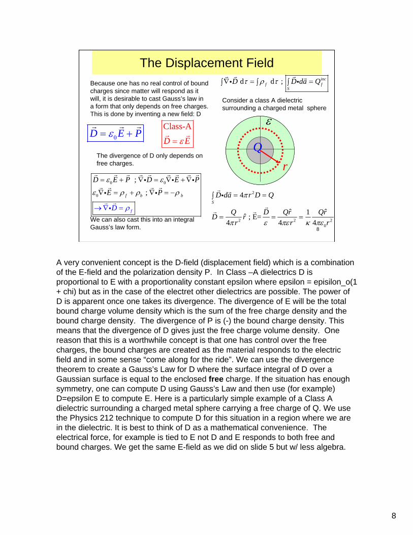
A very convenient concept is the D-field (displacement field) which is a combination of the E-field and the polarization density P. In Class –A dielectrics D is proportional to E with a proportionality constant epsilon where epsilon = episilon_o(1 + chi) but as in the case of the electret other dielectrics are possible. The power of D is apparent once one takes its divergence. The divergence of E will be the total bound charge volume density which is the sum of the free charge density and the bound charge density. The divergence of P is (-) the bound charge density. This means that the divergence of D gives just the free charge volume density. One reason that this is a worthwhile concept is that one has control over the free charges, the bound charges are created as the material responds to the electric field and in some sense “come along for the ride”. We can use the divergence theorem to create a Gauss’s Law for D where the surface integral of D over a Gaussian surface is equal to the enclosed free charge. If the situation has enough symmetry, one can compute D using Gauss’s Law and then use (for example) D=epsilon E to compute E. Here is a particularly simple example of a Class A dielectric surrounding a charged metal sphere carrying a free charge of Q. We use the Physics 212 technique to compute D for this situation in a region where we are in the dielectric. It is best to think of D as a mathematical convenience. The electrical force, for example is tied to E not D and E responds to both free and bound charges. We get the same E-field as we did on slide 5 but w/ less algebra.

9

9

Dielectric around a charged sphere …

2 E usually 4

Hence dielectric reduces E

ˆQ rr

ε επε 0= >

( )0 0

02 2

E 4 4

ˆ ˆ

D E E P P E

Q Qr P rr r

ε ε ε ε

ε επε ε π

= = + → = −

−= → =

b

20b b2 2 2 2

02

02 2

2tot tot

Compute 1 1; 0

4

Surface charge: 4

= 4 4

Q 4 1 1

ˆ ˆ

ˆˆ ˆ ˆb

b

b

PQ r r r

r r r rQP r ra

Q Qa a

Q a Q Q Q

ρε ε

ρ ρε π

ε εσ η

ε π

ε ε χσε π χ π

ε επ σε ε

ε

0 0

0

= −∇

− ∂ ⎧ ⎫= − ∇ ∝ ∇ = =⎨ ⎬∂ ⎩ ⎭

−⎛ ⎞= = − ⎜ ⎟⎝ ⎠

− ⎛ ⎞⎛ ⎞→ = − − ⎜ ⎟⎜ ⎟ 1+⎝ ⎠ ⎝ ⎠⎡ ⎤⎛ ⎞= + = − − → =⎢ ⎥⎜ ⎟

⎝ ⎠⎣ ⎦

i

i i

i i

2tot 24 ; E as before

4ˆ

S

Q QE da r E Q rr

π εε πε0= = = =∫ i

Hence E is reduced inside dielectric due to (-) bound charges on inner dielectric surface.Lets compute the bound charges.

Start by computing P

0 02 2

total 2 2b

Check that total bound charge on a and b is z

; 4 4

er

Q 0

o

inner outerb b

inner outerb b

Q Qa b

a b

ε ε ε εσ σ

ε π ε π

π σ π σ

− −⎛ ⎞ ⎛ ⎞→ = − =⎜ ⎟ ⎜ ⎟⎝ ⎠ ⎝ ⎠

= 4 + 4 =

Q

ε

ra

η

η

−

−

−

−−−

b

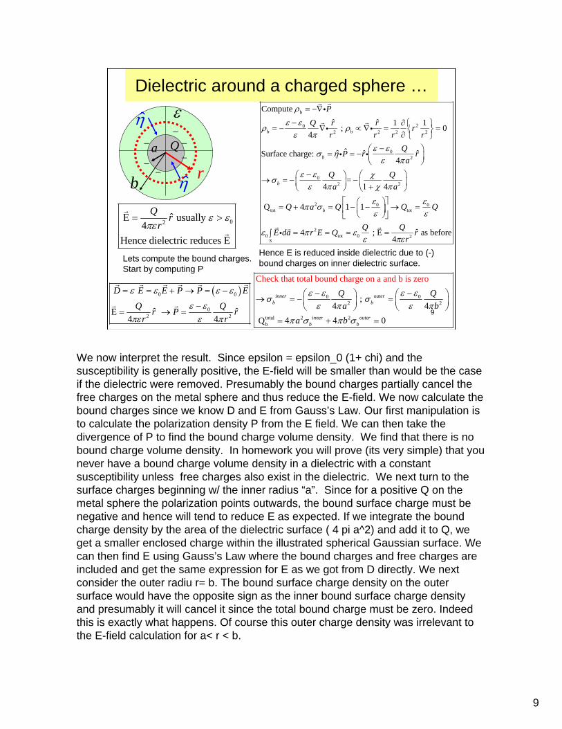
We now interpret the result. Since epsilon = epsilon_0 (1+ chi) and the susceptibility is generally positive, the E-field will be smaller than would be the case if the dielectric were removed. Presumably the bound charges partially cancel the free charges on the metal sphere and thus reduce the E-field. We now calculate the bound charges since we know D and E from Gauss’s Law. Our first manipulation is to calculate the polarization density P from the E field. We can then take the divergence of P to find the bound charge volume density. We find that there is no bound charge volume density. In homework you will prove (its very simple) that you never have a bound charge volume density in a dielectric with a constant susceptibility unless free charges also exist in the dielectric. We next turn to the surface charges beginning w/ the inner radius “a”. Since for a positive Q on the metal sphere the polarization points outwards, the bound surface charge must be negative and hence will tend to reduce E as expected. If we integrate the bound charge density by the area of the dielectric surface ( 4 pi a^2) and add it to Q, we get a smaller enclosed charge within the illustrated spherical Gaussian surface. We can then find E using Gauss’s Law where the bound charges and free charges are included and get the same expression for E as we got from D directly. We next consider the outer radiu r= b. The bound surface charge density on the outer surface would have the opposite sign as the inner bound surface charge density and presumably it will cancel it since the total bound charge must be zero. Indeed this is exactly what happens. Of course this outer charge density was irrelevant to the E-field calculation for a< r < b.

10

10

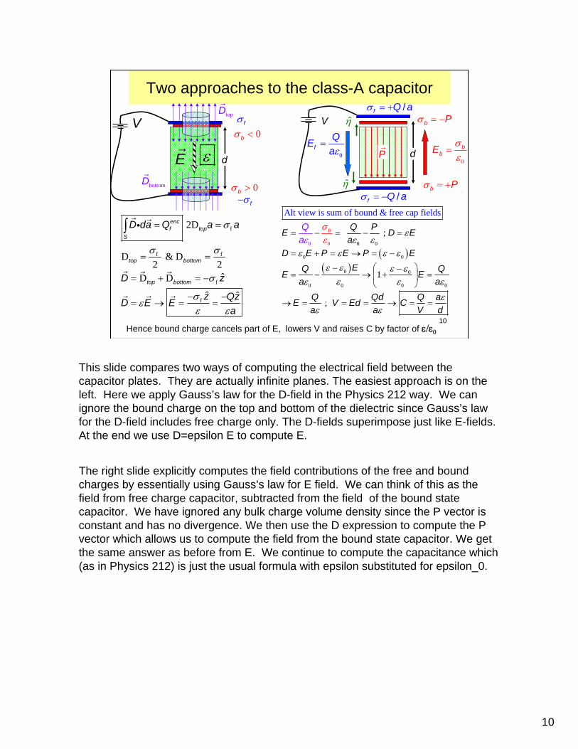
Two approaches to the class-A capacitor

( )( )

0 0

0 0

;

1

;

Alt view is sum of bound & free cap fieldsσε

εε ε

ε ε ε εε ε ε ε

ε ε ε ε

εε ε

ε0 0 0 0

0 0 0 0

= − = − =

= + = → = −

− ⎛ ⎞−= − → + =⎜ ⎟

⎝ ⎠

→ = = = → = =

b Q PE D Ea

D E P E P EEQ QE E

a a

Q Qd Q aE V Ed C

Q

a V

a

a d

Hence bound charge cancels part of E, lowers V and raises C by factor of ε/ε0

b Pσ = −

b Pσ = +

/f Q aσ = +

/f Q aσ = −

bbE σ

ε0

=fQE

aε0

=d

V

η

η

P

0σ >b

σ f

σ− f

d

VtopD

bottomD

εE

0σ <b

f

f f

f

f

2D

D & D2 2

D D ˆ

ˆ ˆ

σ

σ σ

σ

σεε ε

= =

= =

= + = −

− −= → = =

∫ encf top

S

top bottom

top bottom

D da Q a a

D z

z QzD E Ea

i

This slide compares two ways of computing the electrical field between the capacitor plates. They are actually infinite planes. The easiest approach is on the left. Here we apply Gauss’s law for the D-field in the Physics 212 way. We can ignore the bound charge on the top and bottom of the dielectric since Gauss’s law for the D-field includes free charge only. The D-fields superimpose just like E-fields. At the end we use D=epsilon E to compute E.

The right slide explicitly computes the field contributions of the free and bound charges by essentially using Gauss’s law for E field. We can think of this as the field from free charge capacitor, subtracted from the field of the bound state capacitor. We have ignored any bulk charge volume density since the P vector is constant and has no divergence. We then use the D expression to compute the P vector which allows us to compute the field from the bound state capacitor. We get the same answer as before from E. We continue to compute the capacitance which (as in Physics 212) is just the usual formula with epsilon substituted for epsilon_0.

11

11

D is more than a rescaled E

0

somewhere in our loop

2

0

∇ × =

=

→ ∇ × ≠

∫ ∫∫

P da P d

P d RP

P

i i

i

z0 ˆP P z=

R

0

In Class A media D=and one expects D has manyof same properties of electric field.For example both have a Gauss's Law

In electrostatic problems =0but in gene

&

ε

ε

Ε

= =

∇ ×

∫ ∫enc encf tot

S S

D da Q E da Q

E

i i

( )ral 0

The spherical electretis an example where 0

..

ε ε0 0

∇ × ≠

∇ × = ∇ × + = ∇ × + ∇ ×

→ ∇ × = ∇ ×

∇ × ≠

DD E P E P

D PP

Inside sphere z and 0 Outside sphere 0 and 0Evidently 0 on spherical surfaceOf

Bu

c

t where?

ourse the spherical electret is not aClass A dielec

!

tric.

ˆˆ= ∇ × =

= ∇ × =

∇ × ≠

o oP P P zP P

P

Since in general 0We define a potentialfor D such

can as

not -

∇ × ≠

= ∇ D

D

D V

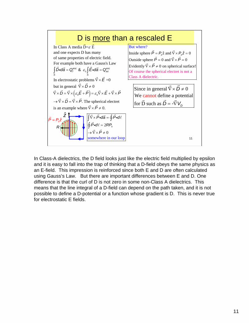
In Class-A dielectrics, the D field looks just like the electric field multiplied by epsilon and it is easy to fall into the trap of thinking that a D-field obeys the same physics as an E-field. This impression is reinforced since both E and D are often calculated using Gauss’s Law. But there are important differences between E and D. One difference is that the curl of D is not zero in some non-Class A dielectrics. This means that the line integral of a D-field can depend on the path taken, and it is not possible to define a D-potential or a function whose gradient is D. This is never truefor electrostatic E fields.

12

12

Perils of using the D –field Gauss’s Law

z0 ˆP P z=

R

r

( ) ( )

( )

( )

3

04

03

0 0

20

220 0

2 10

1

1 3 34 3

3 ; 3

233 34 0

3

ˆ( ) ˆ ˆ ˆ ˆˆ ˆ

ˆ ˆ ˆ cosˆ ˆ

ˆ ˆ cos cos cosˆ ˆ

cos cos

Rp z P

b

b

b

bS

PE R p r r p z r r zR

PD z r r z da rR d d

P P RD da z r z r R d d d d

P RD da d

π

πε ε

φ θ

φ θ θ φ θ

πθ θ

=3

−

⎡ ⎤ ⎡ ⎤= − ⎯⎯⎯⎯⎯→ −⎣ ⎦ ⎣ ⎦

⎡ ⎤= − =⎣ ⎦

⎡ ⎤→ = − =⎣ ⎦

⇒ = =∫ ∫

i i

i

i i i

i

fQ

22

r

Apply Gauss's law to the spherical surface

44

ˆ?f

f f

Q rD da Q r D Q D

rπ

π= → = → =∫ i

2

But the bound charge breaks the spherical symmetry and actually

4ˆf

b

Q rD D

rπ= + bD

R r=R Lets chBut eck if 0 :as expectedf bD da Q D da= =∫ ∫i i

Although the D-field Gauss’s law only depends on free charge, one must be careful in applying it when bound charge is present. In this example we embed a sphere of free charge within our spherical electret with polarization P_0. If we argued that we could still find the E-field using a concentric spherical sphere of radius r since the free charge is spherically symmetric, we would reach the conclusion that D is in the r-hat direction with a Coulomb’s Law magnitude. This is definitely false since we actually have the spherically symmetric Coulomb field due to the spherical free charge, superimposed on the distinctive electret field pattern. We break the spherical symmetry since the electret has cylindrical symmetry about the z-axis rather than spherical symmetry. Our Gauss’s Law conclusion that the integral of D over a sphere is just the free charge is indeed correct, it just doesn’t allow us to compute D or E because of the broken symmetry. We illustrate this for the case of a Gaussian sphere just outside of the R. We can find the D-field of the bound charge by either taking the gradient of our (bound) glued charge potential or recycling the electrical field of an electric dipole with a strength given by P_0 times the volume of the electret sphere as we’ve done here. If set up the D_b da and integrate we find the area integral over D_b vanishes which agrees with the free charge Gauss’s law that applies to the D-field. The moral is that one can only use the D-field Gauss’s Law to compute electric fields if the bound as well as free charges have the desired symmetry. Our simple-minded prediction of a radially symmetric D field for the free charge sphere embedded in a spherical electret went bad since the bound charge did not have spherical symmetry.

13

13

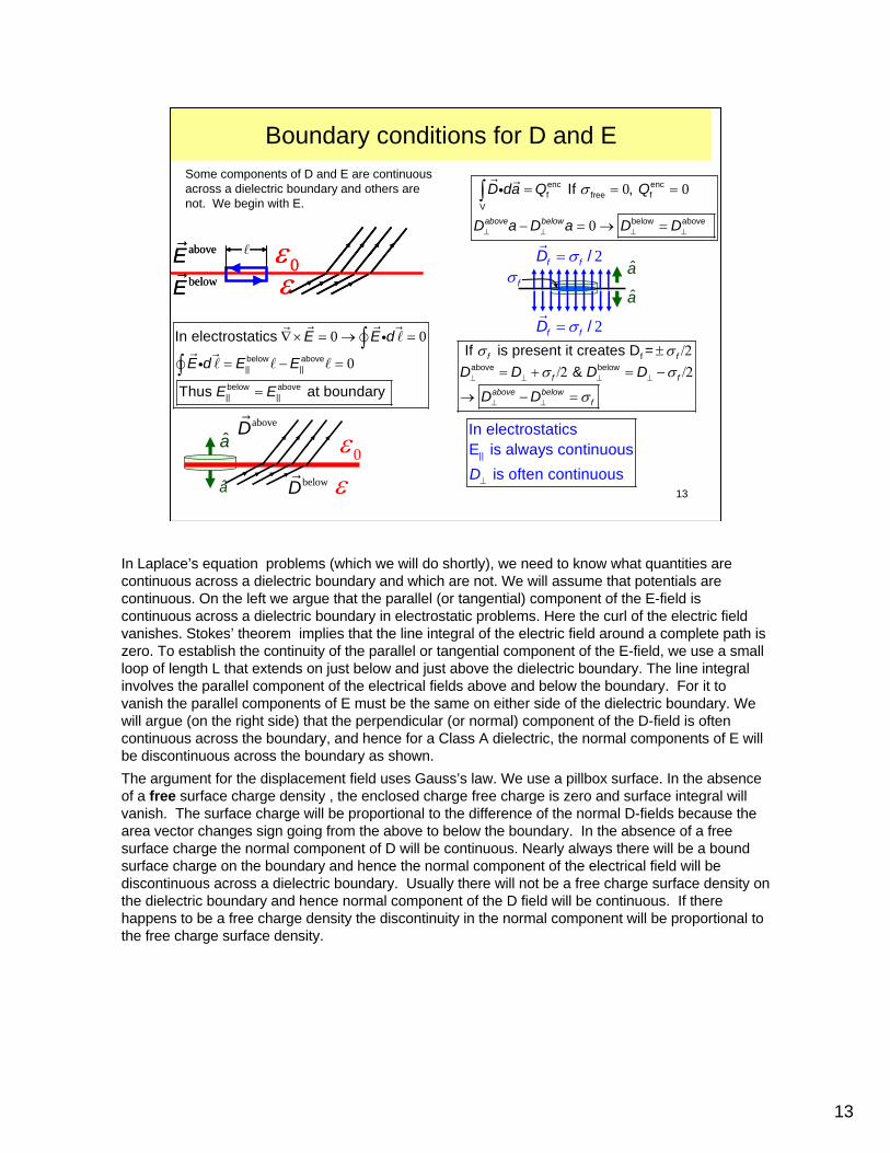
Boundary conditions for D and E

0 0

0below above|| ||

below above|| ||

In electrostatics

Thus at boundary

∇ × = → =

= − =

=

∫∫

E E d

E d E E

E E

i

i

Some components of D and E are continuous across a dielectric boundary and others are not. We begin with E.

2/σ=f fDa

2/σ=f fD

σ f

a

0 0

0

enc encf free f

V

below above

If ,

σ

⊥ ⊥ ⊥ ⊥

= = =

− = → =

∫above below

D da Q Q

D a D a D D

i

fabove below

If is present it creates D = &

σ σσ σ

σ⊥ ⊥ ⊥ ⊥

⊥ ⊥

± /2= + /2 = − /2

→ − =

f f

f f

above belowf

D D D D

D D

||

In electrostaticsE is always continuous

is often continuous⊥D

a

a

0εε

aboveD

belowD

0εε

aboveEbelowE

0εε

aboveEbelowE

In Laplace’s equation problems (which we will do shortly), we need to know what quantities are continuous across a dielectric boundary and which are not. We will assume that potentials are continuous. On the left we argue that the parallel (or tangential) component of the E-field is continuous across a dielectric boundary in electrostatic problems. Here the curl of the electric field vanishes. Stokes’ theorem implies that the line integral of the electric field around a complete path is zero. To establish the continuity of the parallel or tangential component of the E-field, we use a small loop of length L that extends on just below and just above the dielectric boundary. The line integral involves the parallel component of the electrical fields above and below the boundary. For it to vanish the parallel components of E must be the same on either side of the dielectric boundary. We will argue (on the right side) that the perpendicular (or normal) component of the D-field is often continuous across the boundary, and hence for a Class A dielectric, the normal components of E will be discontinuous across the boundary as shown. The argument for the displacement field uses Gauss’s law. We use a pillbox surface. In the absence of a free surface charge density , the enclosed charge free charge is zero and surface integral will vanish. The surface charge will be proportional to the difference of the normal D-fields because the area vector changes sign going from the above to below the boundary. In the absence of a free surface charge the normal component of D will be continuous. Nearly always there will be a bound surface charge on the boundary and hence the normal component of the electrical field will be discontinuous across a dielectric boundary. Usually there will not be a free charge surface density on the dielectric boundary and hence normal component of the D field will be continuous. If there happens to be a free charge density the discontinuity in the normal component will be proportional to the free charge surface density.

14

14

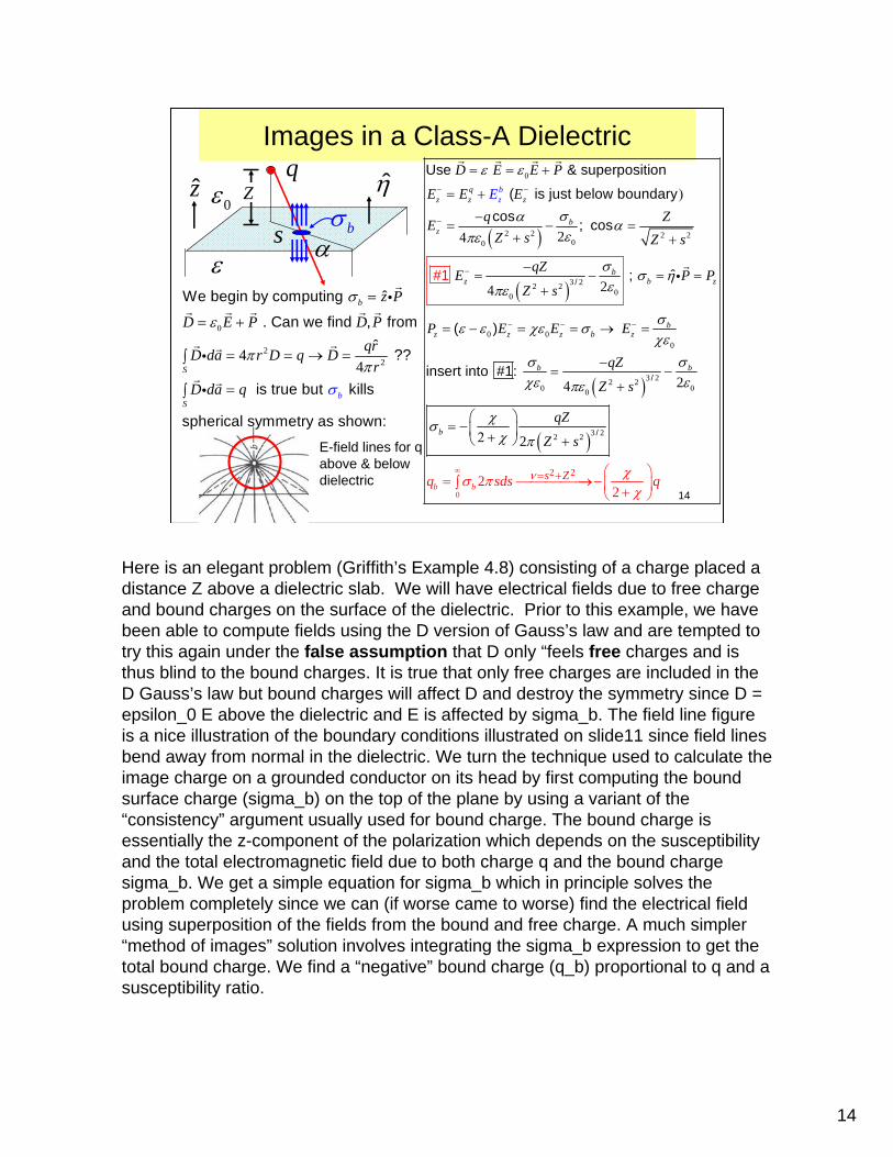
Images in a Class-A Dielectric

224

4

We begin by computing ˆ

. Can we find , fromˆ ??

is true but kills

spherical symmetry as shown:

b

S

bS

z P

D E P D PqrD da r D q D

rD da q

σ

ε

ππ

σ

0

=

= +

= = → =∫

=∫

i

i

i

E-field lines for q above & below dielectric

( )

( )

0

2 2 2 2

3 22 2

0 00

2

2/

Use & superposition

( is just below boundarycos ; cos

ˆ ;

( )

in

#1

sert into #

qz

bzz z

bz

bz b z

bz z z b z

D E E P

E E Eq ZE

Z s Z s

qZE P PZ s

E

P E E E

ε ε

σα αεπε

σσ η

επε

σε ε χε σ

χε

− −

−

00

−

00

− − −

= = +

= + )

−= − =

4 + +

−= − = =

4 +

= − = = → =

i

( )

( )

3 22 20

3 22

0

2

2 2

2

2

2

2

/

/

1: b b

b

b bs Z

qZ

Z s

q

qZ

sds q

Z s

ν

σ σχε επε

χσχ π

χσ πχ

∞

00

= + ⎛ ⎞= ⎯

−= −

4 +

⎛ ⎞= −⎜ ⎟2 +⎝ ⎠

⎯⎯⎯⎯→−⎜ ⎟+⎝ ⎠

+

∫

Z

sε

0εq

bσα

z η

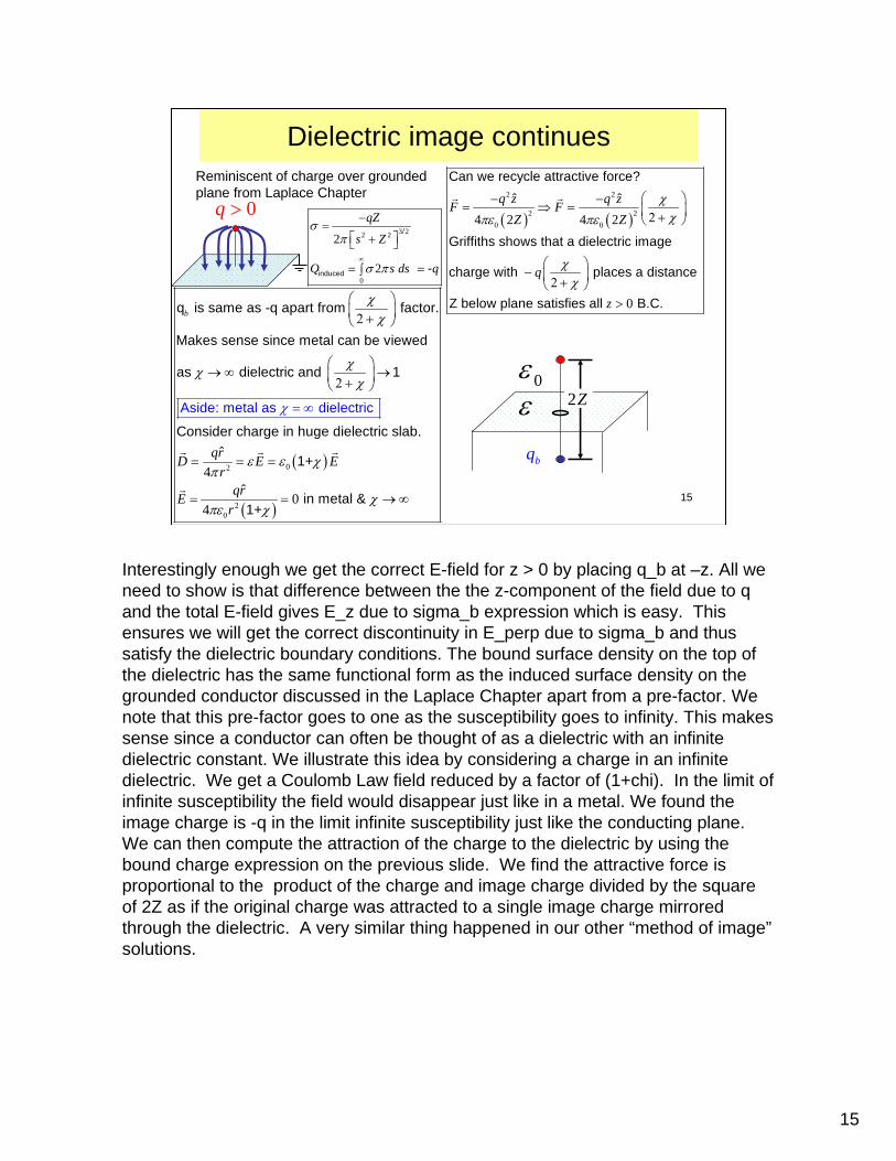
Here is an elegant problem (Griffith’s Example 4.8) consisting of a charge placed a distance Z above a dielectric slab. We will have electrical fields due to free charge and bound charges on the surface of the dielectric. Prior to this example, we have been able to compute fields using the D version of Gauss’s law and are tempted to try this again under the false assumption that D only “feels free charges and is thus blind to the bound charges. It is true that only free charges are included in the D Gauss’s law but bound charges will affect D and destroy the symmetry since D = epsilon_0 E above the dielectric and E is affected by sigma_b. The field line figure is a nice illustration of the boundary conditions illustrated on slide11 since field lines bend away from normal in the dielectric. We turn the technique used to calculate the image charge on a grounded conductor on its head by first computing the bound surface charge (sigma_b) on the top of the plane by using a variant of the “consistency” argument usually used for bound charge. The bound charge is essentially the z-component of the polarization which depends on the susceptibility and the total electromagnetic field due to both charge q and the bound charge sigma_b. We get a simple equation for sigma_b which in principle solves the problem completely since we can (if worse came to worse) find the electrical field using superposition of the fields from the bound and free charge. A much simpler “method of images” solution involves integrating the sigma_b expression to get the total bound charge. We find a “negative” bound charge (q_b) proportional to q and a susceptibility ratio.

15

15

Dielectric image continues

24

q is same as -q apart from factor.

Makes sense since metal can be viewed

as dielectric a

Aside: metal as dielectri

nd 1

Consider charge in huge dielectric slab.

c

ˆ

b

qrDr

χχ

χχχ

ε

χ

π

⎛ ⎞⎜ ⎟2 +⎝ ⎠

⎛ ⎞→ ∞ →⎜ ⎟2 +⎝ ⎠

= ∞

= = ( )

( )

0

2 04

1+

ˆ in metal & 1+

E E

qrEr

ε χ

χπε χ0

=

= = → ∞

0q >3 22 2

0

2

2

/

induced -

qZ

s Z

Q s ds q

σπ

σ π∞

−=

⎡ ⎤+⎣ ⎦

= =∫

Reminiscent of charge over grounded plane from Laplace Chapter

( ) ( )

2 2

2 24 2 4 2

0

Can we recycle attractive force?

ˆ ˆ

Griffiths shows that a dielectric image

charge with places a distance

Z below plane satisfies all B.C.

q z q zF FZ Z

q

z

χχπε πε

χχ

0 0

⎛ ⎞− −= ⇒ = ⎜ ⎟2 +⎝ ⎠

⎛ ⎞− ⎜ ⎟2 +⎝ ⎠

>

2Z

bq

ε0ε

Interestingly enough we get the correct E-field for z > 0 by placing q_b at –z. All we need to show is that difference between the the z-component of the field due to q and the total E-field gives E_z due to sigma_b expression which is easy. This ensures we will get the correct discontinuity in E_perp due to sigma_b and thus satisfy the dielectric boundary conditions. The bound surface density on the top of the dielectric has the same functional form as the induced surface density on the grounded conductor discussed in the Laplace Chapter apart from a pre-factor. We note that this pre-factor goes to one as the susceptibility goes to infinity. This makes sense since a conductor can often be thought of as a dielectric with an infinite dielectric constant. We illustrate this idea by considering a charge in an infinite dielectric. We get a Coulomb Law field reduced by a factor of (1+chi). In the limit of infinite susceptibility the field would disappear just like in a metal. We found the image charge is -q in the limit infinite susceptibility just like the conducting plane. We can then compute the attraction of the charge to the dielectric by using the bound charge expression on the previous slide. We find the attractive force is proportional to the product of the charge and image charge divided by the square of 2Z as if the original charge was attracted to a single image charge mirrored through the dielectric. A very similar thing happened in our other “method of image”solutions.

16

16

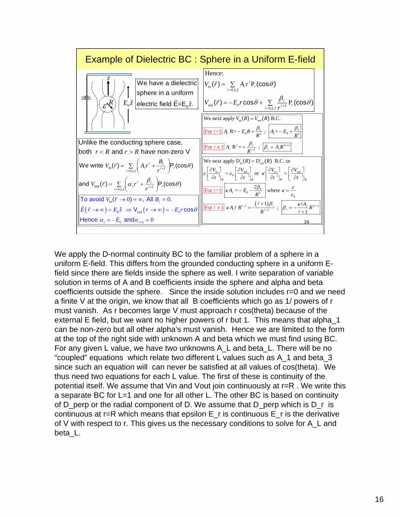
10 1 2

10 1 2

0 0

in, ,

out, ,

in

We write ( ) P (cos )

and ( ) P (

To avoid ( ) , All .

cos )

Unlike the conducting sphere case, both and have non-zero V

V

BV r A rr

E

V r rr

r B

r R r R

θ

βα θ

+=

+=

⎛ ⎞= +∑ ⎜ ⎟⎝ ⎠

→ = ∞

⎛

=

⎞= +∑ ⎜ ⎟⎝ ⎠

< >

( ) ( )0 0

1 0 1 0out V cosˆ

Hence and r E z r E r

E

θ

α α ≠

→ ∞ = ⇒ → ∞ = −

= − =

Example of Dielectric BC : Sphere in a Uniform E-field

in out

1 11 0 1 02 3

2 11

in out

0

We next apply B.C.

R= ; =

R = ;

We next apply D D B.C. or

or

For =

r r r

1

For 1

( ) ( )

( ) ( )

in out in ou

R R R

V R V R

A E R A ER R

A A RR

R R

V V V V

β β

β β

ε ε κ

++

⊥ ⊥

=

− + − +

+ =

=

∂ ∂ ∂ ∂⎡ ⎤ ⎡ ⎤ ⎡ ⎤= =⎢ ⎥ ⎢ ⎥ ⎢ ⎥∂ ∂ ∂⎣ ⎦

≠

⎦ ⎣ ⎦ ⎣

( )

11 0 3

1 2 12

For =1

For

r

2 = where

1 ;

1

1

-

t

R

A ER

AA R RR

β εκ κε

β κκ β

0

− ++≠

⎡ ⎤⎢ ⎥∂⎣ ⎦

− − =

+= = −

+

in0 1 2

out 0 10 1 2

Hence: P

P

, ,

, ,

( ) (cos )

( ) cos (cos )

V r A r

V r E rr

θ

βθ θ

=

+=

= ∑

= − + ∑0

We have a dielectricsphere in a uniform

electric field E=E . zR

z

ε 0 ˆE z

We apply the D-normal continuity BC to the familiar problem of a sphere in a uniform E-field. This differs from the grounded conducting sphere in a uniform E-field since there are fields inside the sphere as well. I write separation of variable solution in terms of A and B coefficients inside the sphere and alpha and beta coefficients outside the sphere. Since the inside solution includes r=0 and we need a finite V at the origin, we know that all B coefficients which go as 1/ powers of r must vanish. As r becomes large V must approach r cos(theta) because of the external E field, but we want no higher powers of r but 1. This means that alpha_1 can be non-zero but all other alpha’s must vanish. Hence we are limited to the form at the top of the right side with unknown A and beta which we must find using BC. For any given L value, we have two unknowns A_L and beta_L. There will be no “coupled” equations which relate two different L values such as A_1 and beta_3 since such an equation will can never be satisfied at all values of cos(theta). We thus need two equations for each L value. The first of these is continuity of the potential itself. We assume that Vin and Vout join continuously at r=R . We write this a separate BC for L=1 and one for all other L. The other BC is based on continuity of D_perp or the radial component of D. We assume that D_perp which is D_r is continuous at r=R which means that epsilon E_r is continuous E_r is the derivative of V with respect to r. This gives us the necessary conditions to solve for A_L and beta_L.

17

17

Completing the dielectric sphere

2 1 2 1

1 1

Now put together the 1 conditions

; 1

; 1+ 01 10

AA R R

AA A

A

κβ β

κ κ

β

+ +

≠ ≠

≠

= = −+

⎛ ⎞→ = − =⎜ ⎟+ +⎝ ⎠= =

0

3

0 2

Putting it all together we havea remarkably simple form:

32

2

cos

cos

in

out

EV r

RV E rr

θκ

κ θκ

−=

+⎡ ⎤−1⎛ ⎞= − −⎢ ⎥⎜ ⎟+⎝ ⎠⎣ ⎦

( ) 311 0 1 1 03

31 011 0 13

1 0 01 0 1

3 301 0 1 0

Put together the 1 conditions

=

2 =2

32 2

3 2 2

A E A E RR

A EA E RR

A E EA E A

E E R E R

β β

κβκ β

κκ

κβ βκ κ

=

− + → = +

+− − → = −

+ −→ + = − → =

+

− −1⎛ ⎞ ⎛ ⎞= + = ⎜ ⎟⎜ ⎟+ +⎝ ⎠⎝ ⎠

0

0

30 0

Hence for there is a constant

3field: 2

For we have the E field added to an ideal dipole with a moment of:

1 4 2

ˆ( ) -

ˆ

ˆ

in

r R

E zE r R V

r R z

p R E z

κ

κ πεκ

<

< = ∇ =+

>

− ⎡ ⎤= ⎣ ⎦+

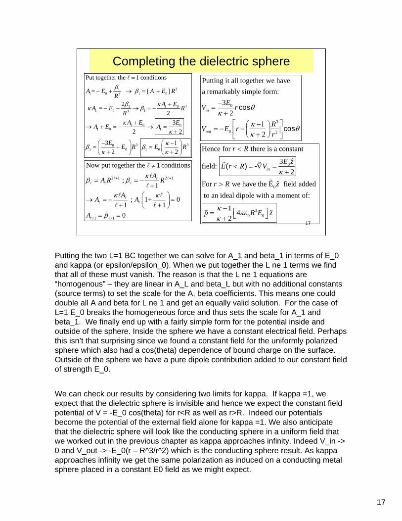
Putting the two L=1 BC together we can solve for A_1 and beta_1 in terms of E_0 and kappa (or epsilon/epsilon_0). When we put together the L ne 1 terms we find that all of these must vanish. The reason is that the L ne 1 equations are “homogenous” – they are linear in A_L and beta_L but with no additional constants (source terms) to set the scale for the A, beta coefficients. This means one could double all A and beta for L ne 1 and get an equally valid solution. For the case of L=1 E_0 breaks the homogeneous force and thus sets the scale for A_1 and beta_1. We finally end up with a fairly simple form for the potential inside and outside of the sphere. Inside the sphere we have a constant electrical field. Perhaps this isn’t that surprising since we found a constant field for the uniformly polarized sphere which also had a cos(theta) dependence of bound charge on the surface. Outside of the sphere we have a pure dipole contribution added to our constant field of strength E_0.

We can check our results by considering two limits for kappa. If kappa =1, we expect that the dielectric sphere is invisible and hence we expect the constant field potential of V = -E_0 cos(theta) for r<R as well as r>R. Indeed our potentials become the potential of the external field alone for kappa =1. We also anticipate that the dielectric sphere will look like the conducting sphere in a uniform field that we worked out in the previous chapter as kappa approaches infinity. Indeed V_in -> 0 and V_out -> -E_0(r – R^3/r^2) which is the conducting sphere result. As kappa approaches infinity we get the same polarization as induced on a conducting metal sphere placed in a constant E0 field as we might expect.

18

18

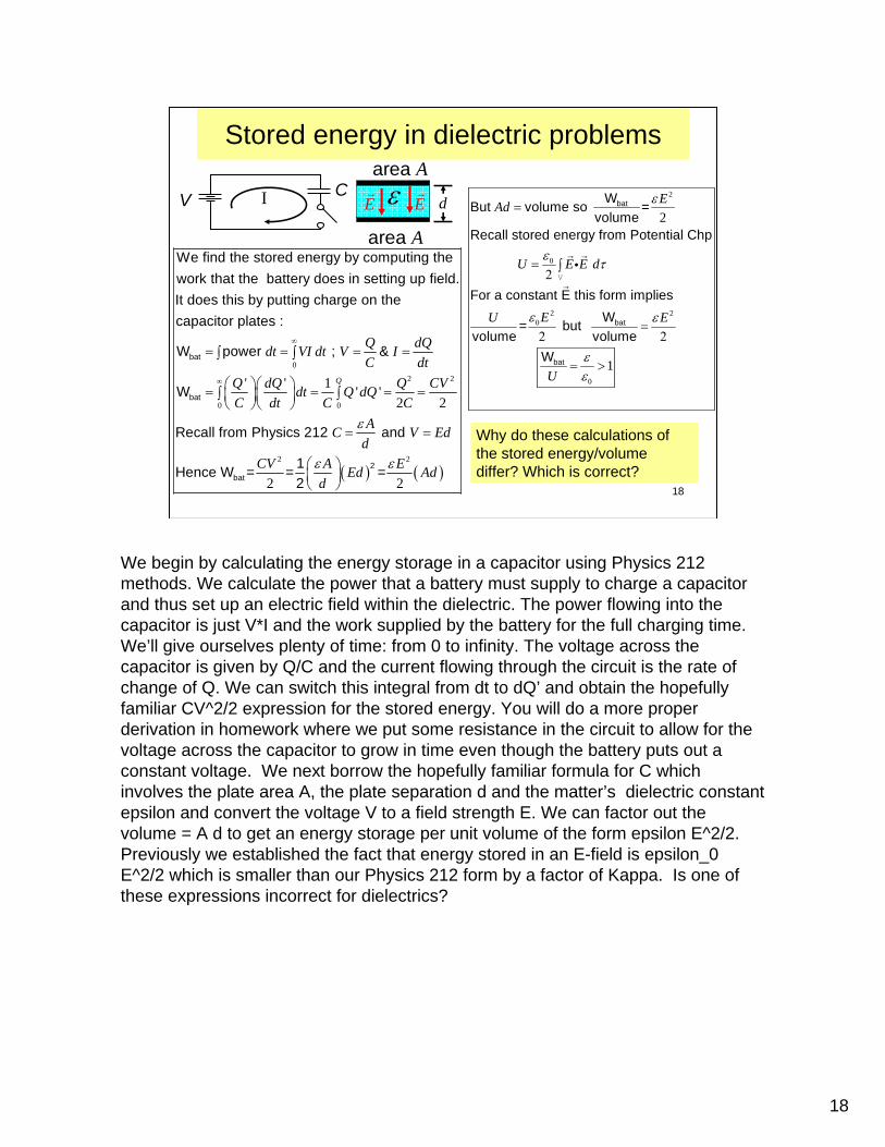
Stored energy in dielectric problems

0

' '

bat

bat

We find the stored energy by computing the work that the battery does in setting up field.It does this by putting charge on thecapacitor plates :

W power ; &

W

Q dQdt VI dt V IC dt

Q dQC d

∞

= = = =∫ ∫

⎛ ⎞= ⎜ ⎟⎝ ⎠

( ) ( )

2 2

0 0

2 2

1 ' '2 2

2 22

bat

Recall from Physics 212 and

1Hence W = = = 2

Q Q CVdt Q dQt C C

AC V Edd

CV A EEd Add

ε

ε ε

∞ ⎛ ⎞ = = =∫ ∫⎜ ⎟⎝ ⎠

= =

⎛ ⎞⎜ ⎟⎝ ⎠

V I C εarea A

area A

dE E2

2 2

2

1

bat

bat

bat

WBut volume so =volume

Recall stored energy from Potential Chp

For a constant E this form impliesW= but

volume volumeW

EAd

U E E d

EU E

U

ε

ε τ

ε ε

εε

0

0

0

=

= ∫2

=2 2

= >

iV

Why do these calculations of the stored energy/volume differ? Which is correct?

We begin by calculating the energy storage in a capacitor using Physics 212 methods. We calculate the power that a battery must supply to charge a capacitor and thus set up an electric field within the dielectric. The power flowing into the capacitor is just V*I and the work supplied by the battery for the full charging time. We’ll give ourselves plenty of time: from 0 to infinity. The voltage across the capacitor is given by Q/C and the current flowing through the circuit is the rate of change of Q. We can switch this integral from dt to dQ’ and obtain the hopefully familiar CV^2/2 expression for the stored energy. You will do a more proper derivation in homework where we put some resistance in the circuit to allow for the voltage across the capacitor to grow in time even though the battery puts out a constant voltage. We next borrow the hopefully familiar formula for C which involves the plate area A, the plate separation d and the matter’s dielectric constant epsilon and convert the voltage V to a field strength E. We can factor out the volume = A d to get an energy storage per unit volume of the form epsilon E^2/2. Previously we established the fact that energy stored in an E-field is epsilon_0 E^2/2 which is smaller than our Physics 212 form by a factor of Kappa. Is one of these expressions incorrect for dielectrics?

19

19

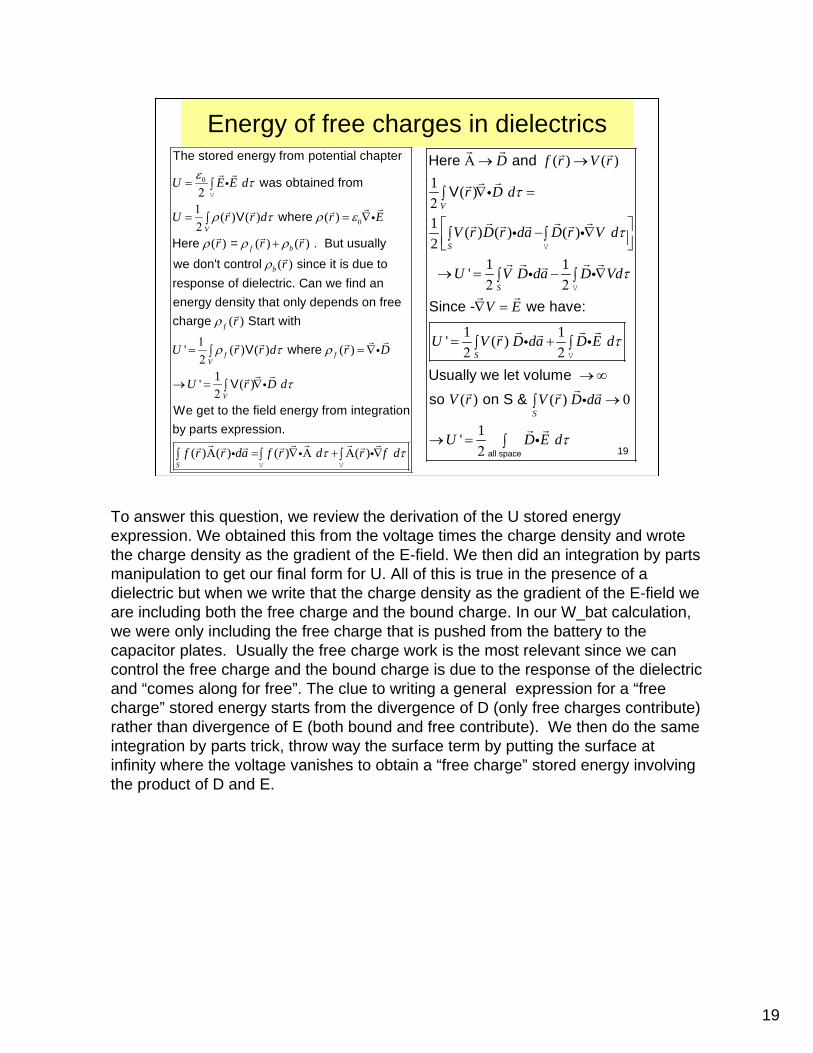
Energy of free charges in dielectrics

( ) ( ) ( )

( ) ( ) ( )

( )

The stored energy from potential chapter

was obtained from

V where

Here = . But usuallywe don't control since it is due torespon

V

f b

b

U E E d

U r r d r E

r r r

r

ε τ

ρ τ ρ ε

ρ ρ ρ

ρ

0

0

= ∫21

= = ∇∫2

+

i

i

V

( )

' ( ) ( ) ( )

1' ( )

se of dielectric. Can we find an energy density that only depends on freecharge Start with

V where

V

We get to the field energy from integrat

f

f fV

V

r

U r r d r D

U r D d

ρ

ρ τ ρ

τ

1= = ∇∫

2

→ = ∇∫2

i

i

( ) ( ) ( ) ( )

ionby parts expression.

S

f r r da f r d r f dτ τΑ = ∇ Α + Α ∇∫ ∫ ∫i i iV V

( ) ( )1 ( )

1 ( ) ( ) ( )2

1 1'

1 1' ( )

(

Here and

V

Since - we have:

Usually we let volume so

V

S

S

S

D f r V r

r D d

V r D r da D r V d

U V D da D Vd

V E

U V r D da D E d

V r

τ

τ

τ

τ

Α → →

∇ =∫2

⎡ ⎤− ∇∫ ∫⎢ ⎥⎣ ⎦

→ = − ∇∫ ∫2 2

∇ =

= +∫ ∫2 2

→ ∞

i

i i

i i

i i

V

V

V

) ( ) 0

1'all space

on S &

SV r D da

U D E dτ

→∫

→ = ∫2

i

i

To answer this question, we review the derivation of the U stored energy expression. We obtained this from the voltage times the charge density and wrote the charge density as the gradient of the E-field. We then did an integration by parts manipulation to get our final form for U. All of this is true in the presence of a dielectric but when we write that the charge density as the gradient of the E-field we are including both the free charge and the bound charge. In our W_bat calculation, we were only including the free charge that is pushed from the battery to the capacitor plates. Usually the free charge work is the most relevant since we can control the free charge and the bound charge is due to the response of the dielectric and “comes along for free”. The clue to writing a general expression for a “free charge” stored energy starts from the divergence of D (only free charges contribute) rather than divergence of E (both bound and free contribute). We then do the same integration by parts trick, throw way the surface term by putting the surface at infinity where the voltage vanishes to obtain a “free charge” stored energy involving the product of D and E.

20

20

U versus U’

1' .

1'

all space

all space

Griffith's discusses incremental change

in U' since D depend history of how

E was applied:

Usually:

can

U D E d

U D E d

τ

τ

Δ = Δ∫2

= ∫2

i

i

( )12

0

1

'2 2

' '

Now lets compute

and as before

U differs form U' since U' doesn't include(negative) work on the bound charges.

U E E d

Q Q Q AU Ad UA A Ad

U U UU

ε τ

ε ε εεε ε ε ε

εε

0

−0 0 0

= ∫2

⎛ ⎞ ⎛ ⎞= = =⎜ ⎟ ⎜ ⎟⎝ ⎠ ⎝ ⎠

⎛ ⎞→ = >⎜ ⎟

⎝ ⎠

i

( )12 2 2

1'

1'2 2 2 2

Lets compute U D E d

Q Q Q a Q CVU adA A Ad C

τ

εε

−

= ∫2

⎛ ⎞ ⎛ ⎞= = = =⎜ ⎟ ⎜ ⎟⎝ ⎠ ⎝ ⎠

i

Using Gauss's law:

& Q QD EA Aε

= =

0σ >b

σf

σ− f

d

VtopD

bottomD

εE

0σ <b

I

Here we apply the U’ expression to the usual dielectric capacitor but this time we concentrate on expressions in terms of the free charge on the capacitor plates rather than the work supplied by the battery to give us more practice in dealing with D. Our first step is to compute D_top using Gauss’s Law for the free charge on the top plate and D_bottom using Gauss’s law for free charge on the bottom plate. The total D is the sum of D_top + D_bottom and is just Q/A where again Q is just the free charge. We are assuming a linear medium so D= epsilon E which allows us to calculate E. We then can compute U’ from our integral expression involving D and E which is simple since the D dot E integrand is constant and the volume is just A d. Putting it altogether we get the Physics 212 expression for the stored energy in a capacitor. If we next compute the stored energy of the free plus bound charge we get a smaller stored energy. This is somewhat surprising that it takes less work to supply the capacitor with bound plus free charge than free charge alone. Evidently it takes negative work to create the bound charge. The reason is that bound charge on the top plate is negative and the bound charge on the bottom plate is positive which is the opposite of the free charge. This must be true since the E field in the dielectric is smaller than you get with no dielectric for the same Q so the bound charge field opposes the free charge field . Hence takes negative work to put a negative bound charge on the top plate and a positive bound charge on the bottom plate since this is the direction bound charges would like to move in a downward E-field. Is it always true that U’ > U?

21

21

U versus U’ on Electret

20 0

002 2

ˆ ˆCompute U= σε τ τ

ε ε ε0 0

= = ⇒ =∫ b P PE E d E z z Ui

00

00

0 0

E DNow : ' 2

ˆ ˆ ˆ ;

ˆ ˆ

Surprise!! '

τ

σε ε

ε εε

0 0

0 00

=

= = − = −

⎛ ⎞= − = − +⎜ ⎟

⎝ ⎠

→ = → =

∫b

U d

PP P z E z z

PD E P z P z

D U

i

0b Pσ = −

0b Pσ = +z η

η

ˆbE zσε0

= −

0D

D

Work =U' is energy to assemble the free charges. Here there are no fre Woe ch rkarges. '→ = =U

0

Electric slab

ithˆ

w=P P z

( )2

2 30

20 0

30

0

00

0 0 02 3

0

0 0

0 42

23 3 2 9

49 2

02

73

7

4

ˆ ˆˆ- '

' ' Evidently

' ' '

.

ε εε ε

πε

ε

ε

τε

τ

ππ

ε

0 0

<

> < >>

>

⎛ ⎞= + = + = + → = = −⎜ ⎟

⎝ ⎠⎛ ⎞

= = − =⎜ ⎟⎝ ⎠

= = + =

−

→ +∫

r R

r R r R r Rr R

r R

P z P z PD

P R

ED E P P z u

P RU P Ru

U d E E U U

i

i

0

03

For Spherical Electretˆ

( ) -ε

< =P zE r R

Why is U'=0

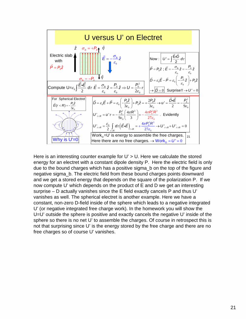
Here is an interesting counter example for U’ > U. Here we calculate the stored energy for an electret with a constant dipole density P. Here the electric field is only due to the bound charges which has a positive sigma_b on the top of the figure and negative sigma_b. The electric field from these bound charges points downward and we get a stored energy that depends on the square of the polarization P. If we now compute U’ which depends on the product of E and D we get an interesting surprise – D actually vanishes since the E field exactly cancels P and thus U’vanishes as well. The spherical electret is another example. Here we have a constant, non-zero D-field inside of the sphere which leads to a negative integrated U’ (or negative integrated free charge work). In the homework you will show the U=U’ outside the sphere is positive and exactly cancels the negative U’ inside of the sphere so there is no net U’ to assemble the charges. Of course in retrospect this is not that surprising since U’ is the energy stored by the free charge and there are no free charges so of course U’ vanishes.

22

22

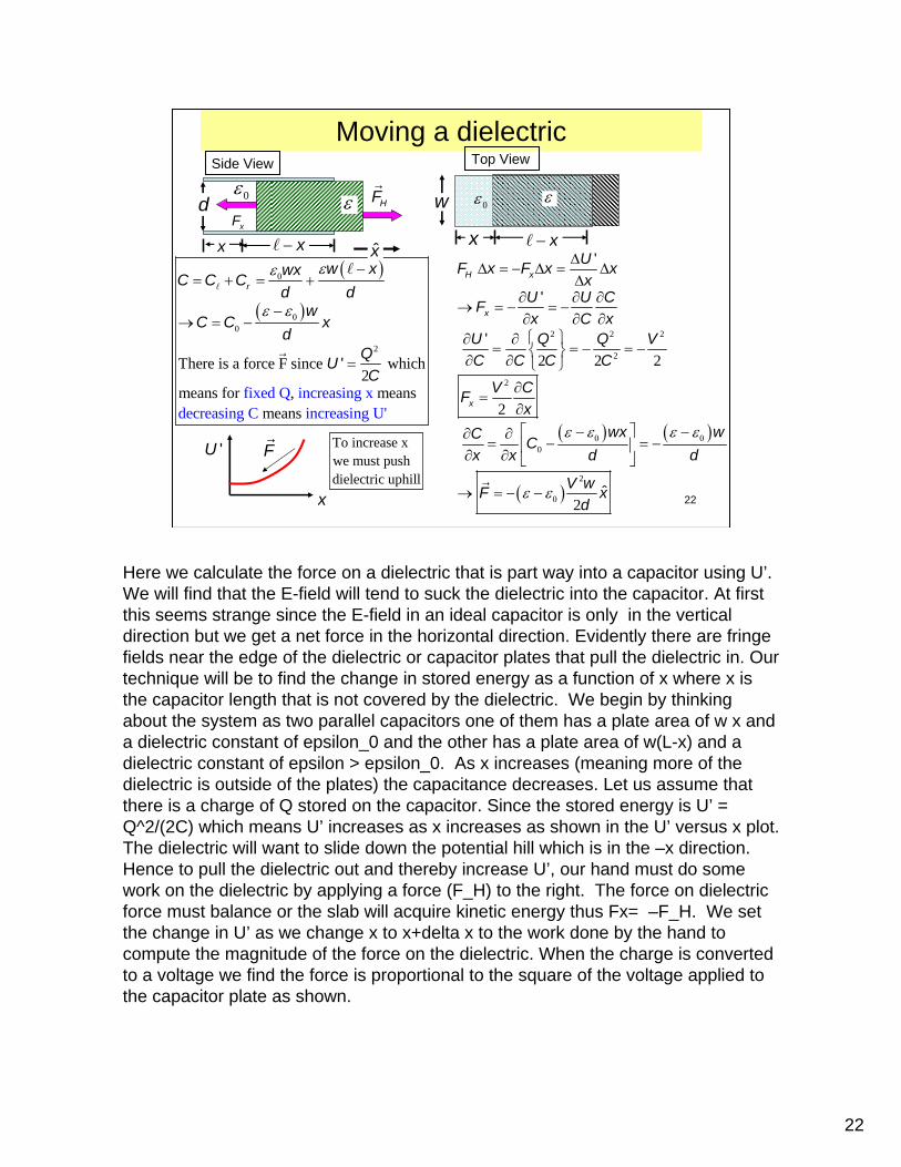
Moving a dielectric

x−x

ε0εw

( )

( )0

2

There is a force F since whic

fixed

h2

means for , Q increasing xdecreasing C incre

means means asing U'

'

εε

ε ε

0

0

−= + = +

−→ = −

=

r

w xwxC C Cd d

wC C x

dQUC

'U

x

F To increase xwe must pushdielectric uphill

( ) ( )

( )

2 2 2

2

2

0

2

2 2 2

2

2

'

'

'

ˆ

ε ε ε ε

ε ε

0 0

0

ΔΔ = − Δ = Δ

Δ∂ ∂ ∂

→ = − = −∂ ∂ ∂⎧ ⎫∂ ∂

= = − = −⎨ ⎬∂ ∂ ⎩ ⎭∂

=∂⎡ ⎤− −∂ ∂

= − = −⎢ ⎥∂ ∂ ⎣ ⎦

→ = − −

H x

x

x

UF x F x xx

U U CFx C x

U Q Q VC C C C

V CFx

wx wC Cx x d d

V wF xd

ε0εHF

xFd

x− xx

Side View Top View

Here we calculate the force on a dielectric that is part way into a capacitor using U’. We will find that the E-field will tend to suck the dielectric into the capacitor. At first this seems strange since the E-field in an ideal capacitor is only in the vertical direction but we get a net force in the horizontal direction. Evidently there are fringe fields near the edge of the dielectric or capacitor plates that pull the dielectric in. Our technique will be to find the change in stored energy as a function of x where x is the capacitor length that is not covered by the dielectric. We begin by thinking about the system as two parallel capacitors one of them has a plate area of w x and a dielectric constant of epsilon_0 and the other has a plate area of w(L-x) and a dielectric constant of epsilon > epsilon_0. As x increases (meaning more of the dielectric is outside of the plates) the capacitance decreases. Let us assume that there is a charge of Q stored on the capacitor. Since the stored energy is U’ = Q^2/(2C) which means U’ increases as x increases as shown in the U’ versus x plot. The dielectric will want to slide down the potential hill which is in the –x direction. Hence to pull the dielectric out and thereby increase U’, our hand must do some work on the dielectric by applying a force (F_H) to the right. The force on dielectric force must balance or the slab will acquire kinetic energy thus Fx= –F_H. We set the change in U’ as we change x to x+delta x to the work done by the hand to compute the magnitude of the force on the dielectric. When the charge is converted to a voltage we find the force is proportional to the square of the voltage applied to the capacitor plate as shown.

23

23

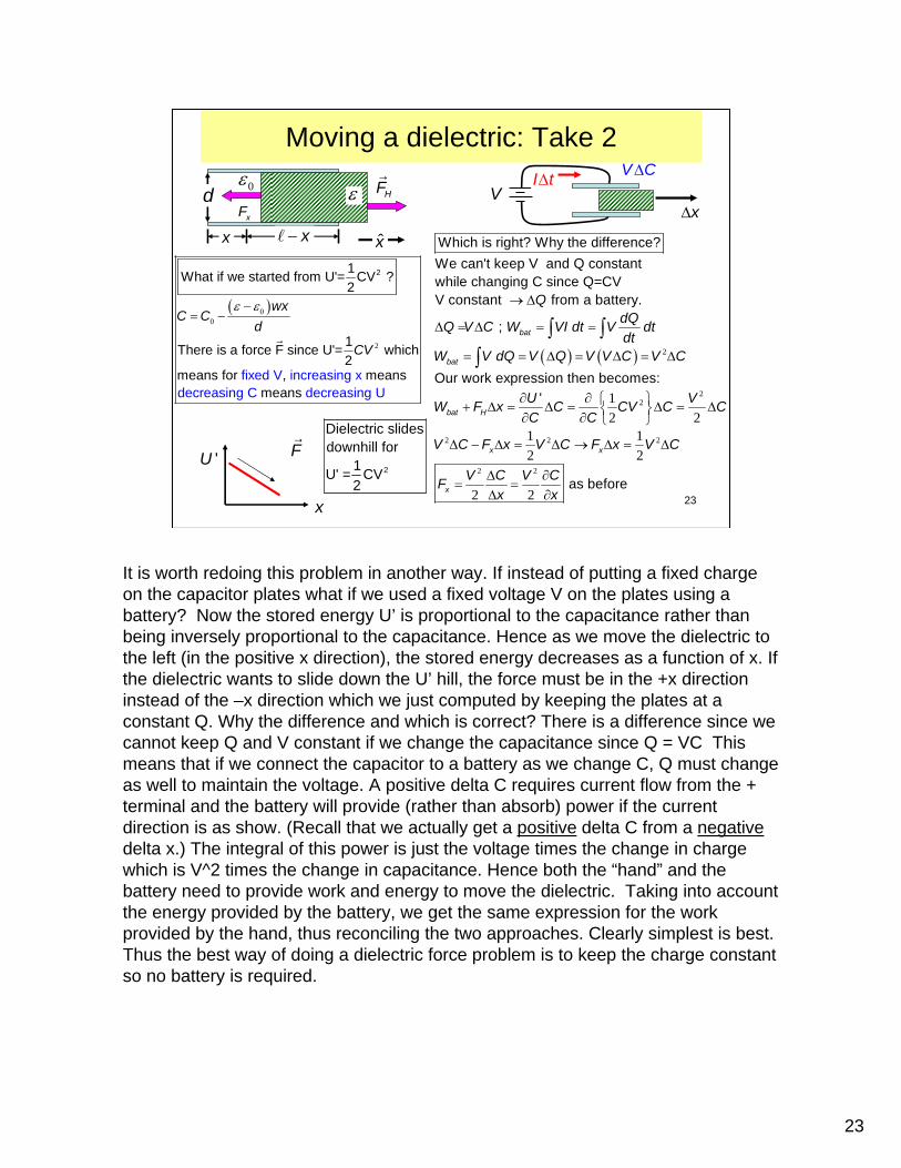
Moving a dielectric: Take 2

( )0

2

21What if we started from U'= CV ?2

1There is a force F since U'= which2

fixed V increasimeans for , meng xdecreasing C

ans mea decreasing Uns

ε ε0−= −

wxC C

d

CV

ε0εHF

xFd

x− xx

'U

x

F2

Dielectric slidesdownhill for

1U' = CV 2

( ) ( ) 2

Which is right? Why the difference?We can't keep V and Q constantwhile changing C since Q=CVV constant from a battery.

;

Our work expression then b

→ Δ

Δ = Δ = =

= = Δ = Δ = Δ

∫ ∫∫

bat

bat

QdQQ V C W VI dt V dtdt

W V dQ V Q V V C V C

22

2 2 2

2 2

12 2

1 12 2

2 2

ecomes:'

as before

∂ ∂ ⎧ ⎫+ Δ = Δ = Δ = Δ⎨ ⎬∂ ∂ ⎩ ⎭

Δ − Δ = Δ → Δ = Δ

Δ ∂= =

Δ ∂

bat H

x x

x

U VW F x C CV C CC C

V C F x V C F x V C

V C V CFx x

ΔI tV

Δx

ΔV C

It is worth redoing this problem in another way. If instead of putting a fixed charge on the capacitor plates what if we used a fixed voltage V on the plates using a battery? Now the stored energy U’ is proportional to the capacitance rather than being inversely proportional to the capacitance. Hence as we move the dielectric to the left (in the positive x direction), the stored energy decreases as a function of x. If the dielectric wants to slide down the U’ hill, the force must be in the +x direction instead of the –x direction which we just computed by keeping the plates at a constant Q. Why the difference and which is correct? There is a difference since we cannot keep Q and V constant if we change the capacitance since Q = VC This means that if we connect the capacitor to a battery as we change C, Q must change as well to maintain the voltage. A positive delta C requires current flow from the + terminal and the battery will provide (rather than absorb) power if the current direction is as show. (Recall that we actually get a positive delta C from a negativedelta x.) The integral of this power is just the voltage times the change in charge which is V^2 times the change in capacitance. Hence both the “hand” and the battery need to provide work and energy to move the dielectric. Taking into account the energy provided by the battery, we get the same expression for the work provided by the hand, thus reconciling the two approaches. Clearly simplest is best. Thus the best way of doing a dielectric force problem is to keep the charge constant so no battery is required.