Electron Spin Resonance

Eric ReichweinBryce Burgess

Department of PhysicsUniversity of California, Santa Cruz

February 24, 2014

Abstract

We studied electron spin resonance in diphenyl-picril-hydrazyl (DPPH). We choseDPPH for the one unpaired free radical (free electron). Using a reflex klystron weproduced microwave radiation measured the interference of signal that was purelyreflected and a signal that was reflected (or absorbed) by DPPH. We determinedthe radiation frequency to be ν = 9.253 GHz. The external magnetic field had somehysteresis effect. During the up swing resonance occurred when Bext = 3201± 1Gaussand on the down swing resonance occurred when Bext = 3199± 1Gauss. From here weused semi-classical mechanics to derive the Lande g-factor to be g = 2.0659± 0.0655which was about 3% of the established value of g = 2.0036.

1

Contents

1 Introduction 31.1 Historical Background . . . . . . . . . . . . . . . . . . . . . . . . . . . . . . 3

1.1.1 Zeeman Effect . . . . . . . . . . . . . . . . . . . . . . . . . . . . . . . 31.1.2 Stern-Gerlach Experiment . . . . . . . . . . . . . . . . . . . . . . . . 31.1.3 Uhlenbeck-Goudsmit Postulate of Spin and The Dirac Equation . . . 41.1.4 First Observation of ESR and Applications . . . . . . . . . . . . . . . 4

1.2 Physics of ESR . . . . . . . . . . . . . . . . . . . . . . . . . . . . . . . . . . 5

2 Procedures and Setup 62.1 The Reflex Klystron (1) and Isolator (1) . . . . . . . . . . . . . . . . . . . . 62.2 The Wave Meter (2) and Terminator (2) . . . . . . . . . . . . . . . . . . . . 72.3 The Magic Tee (3,7) . . . . . . . . . . . . . . . . . . . . . . . . . . . . . . . 72.4 The Attenuator (4,6) and Phase Shifter (5) . . . . . . . . . . . . . . . . . . . 72.5 The Sample and Magnet (5) . . . . . . . . . . . . . . . . . . . . . . . . . . . 82.6 The Diode Detector (8) . . . . . . . . . . . . . . . . . . . . . . . . . . . . . . 8

3 Data and Analysis 83.1 The Wave Meter Q Factor . . . . . . . . . . . . . . . . . . . . . . . . . . . . 83.2 Rectangular Wave Guide Cut Off Frequency Calculations . . . . . . . . . . . 93.3 Determination of Lande g-Factor . . . . . . . . . . . . . . . . . . . . . . . . 10

4 Conclusion 12

2

1 Introduction

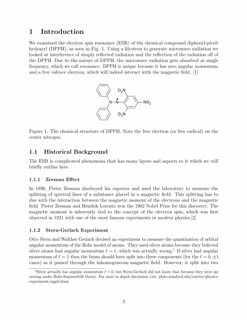
We examined the electron spin resonance (ESR) of the chemical compound diphenyl-picril-hydrazyl (DPPH), as seen in Fig. 1. Using a klystron to generate microwave radiation welooked at interference of simply reflected radiation and the reflection of the radiation off ofthe DPPH. Due to the nature of DPPH, the microwave radiation gets absorbed at singlefrequency, which we call resonance. DPPH is unique because it has zero angular momentum,and a free valence electron, which will indeed interact with the magnetic field. [1]

Figure 1: The chemical structure of DPPH. Note the free electron (or free radical) on thecenter nitrogen.

1.1 Historical Background

The ESR is complicated phenomena that has many layers and aspects to it which we willbriefly outline here.

1.1.1 Zeeman Effect

In 1896, Pieter Zeeman disobeyed his superior and used the laboratory to measure thesplitting of spectral lines of a substance placed in a magnetic field. This splitting has todue with the interaction between the magnetic moment of the electrons and the magneticfield. Pieter Zeeman and Hendrik Lorentz won the 1902 Nobel Prize for this discovery. Themagnetic moment is inherently tied to the concept of the electron spin, which was firstobserved in 1921 with one of the most famous experiments in modern physics.[2]

1.1.2 Stern-Gerlach Experiment

Otto Stern and Walther Gerlach devised an experiment to measure the quantization of orbitalangular momentum of the Bohr model of atoms. They used silver atoms because they believedsilver atoms had angular momentum ` = 1, which was actually wrong.1 If silver had angularmomentum of ` = 1 then the beam should have split into three components (for the ` = 0,±1cases) as it passed through the inhomogeneous magnetic field. However, it split into two

1Silver actually has angular momentum ` = 0, but Stern-Gerlach did not know that because they were op-erating under Bohr-Sommerfeld thoery. For more in depth discussion vist: plato.stanford.edu/entries/physics-experiment/app5.html.

3

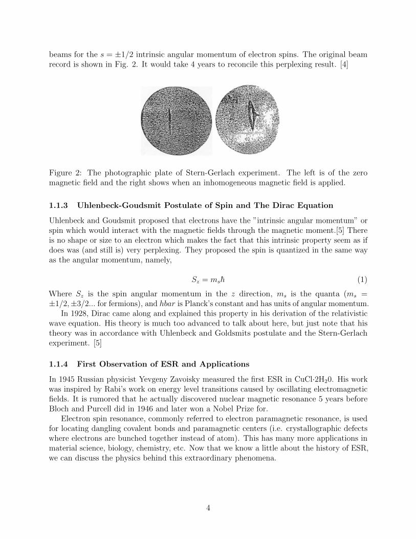
beams for the s = ±1/2 intrinsic angular momentum of electron spins. The original beamrecord is shown in Fig. 2. It would take 4 years to reconcile this perplexing result. [4]

Figure 2: The photographic plate of Stern-Gerlach experiment. The left is of the zeromagnetic field and the right shows when an inhomogeneous magnetic field is applied.

1.1.3 Uhlenbeck-Goudsmit Postulate of Spin and The Dirac Equation

Uhlenbeck and Goudsmit proposed that electrons have the ”intrinsic angular momentum” orspin which would interact with the magnetic fields through the magnetic moment.[5] Thereis no shape or size to an electron which makes the fact that this intrinsic property seem as ifdoes was (and still is) very perplexing. They proposed the spin is quantized in the same wayas the angular momentum, namely,

Sz = msh̄ (1)

Where Sz is the spin angular momentum in the z direction, ms is the quanta (ms =±1/2,±3/2... for fermions), and hbar is Planck’s constant and has units of angular momentum.

In 1928, Dirac came along and explained this property in his derivation of the relativisticwave equation. His theory is much too advanced to talk about here, but just note that histheory was in accordance with Uhlenbeck and Goldsmits postulate and the Stern-Gerlachexperiment. [5]

1.1.4 First Observation of ESR and Applications

In 1945 Russian physicist Yevgeny Zavoisky measured the first ESR in CuCl·2H20. His workwas inspired by Rabi’s work on energy level transitions caused by oscillating electromagneticfields. It is rumored that he actually discovered nuclear magnetic resonance 5 years beforeBloch and Purcell did in 1946 and later won a Nobel Prize for.

Electron spin resonance, commonly referred to electron paramagnetic resonance, is usedfor locating dangling covalent bonds and paramagnetic centers (i.e. crystallographic defectswhere electrons are bunched together instead of atom). This has many more applications inmaterial science, biology, chemistry, etc. Now that we know a little about the history of ESR,we can discuss the physics behind this extraordinary phenomena.

4

1.2 Physics of ESR

The main point of this lab is measure the dimensionless Lande g factor. This is a quantityinherently tied to quantum mechanics (specifically quantum electrodynamics). It arises fromthe fact the electron has the intrinsic angular momentum called spin. Due to this propertythe electron also has a magnetic moment µ, which is anti-parallel to the spin vector.[6] Themagnetic moment in the z direction is given in relation to Eq. 1 as

µz = g

(q

2me

)Sz = g

(q

2me

)msh̄ = gµbms (2)

Where µb = (qh̄/2me) is called the Bohr Magneton. Going further and recalling thepotential energy between a magnetic field and magnetic moment ,U = −µ ·B, we can calculatethe energy difference between the two quantum states (namely, spin parallel and antiparallelto external magnetic field),

U = −µz ·B = −gµbmsB cos θ (3)

And now we look at the energy difference,

(4)∆U = −gµbmsB cos(π)− (−gµbmsB cos(0))

= 2gµbmsB= gµbB

Where in the last step we invoked the condition of ms = 1/2 and we have handled itssign previously in the derivation. Now we can probe this quantized energy difference byshooting photons with energy that are precisely equal to the energy difference of the quantumstates. If we apply a magnetic field the electrons will tend to align themselves parallel tothe magnetic field because that is the low energy state. The photons will be absorbed bythe electrons and flip the electron to the higher energy state. This only happens at a veryprecise photon energy (or frequency). We can determine what frequency this needs to be atby equating the the change in electron energy to photon energy,

E = h̄ω= ∆U= gµbB

Therefore,

ω =gµbB

h̄=gqB

2me

(5)

Equation 5 tells us resonant frequency of the klystron (and consequently the photons) toobserve electron spin resonance in DPPH. Once we determine this we can conclude what theLande g factor is by rearranging Eq. 5,

ω =gqB

2me

−→ g =2meω

qB(6)

5

2 Procedures and Setup

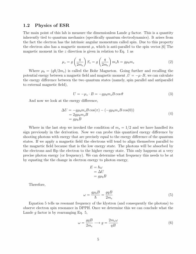
The bulk of this experiment was based on the setup and tuning of the apparatus so we shallspend a good portion of this lab report describing the setup in detail. In Fig. 3 we havelabeled each part of the apparatus in numerical order of the power propagation.

Figure 3: The schematic of the ESR apparatus.

2.1 The Reflex Klystron (1) and Isolator (1)

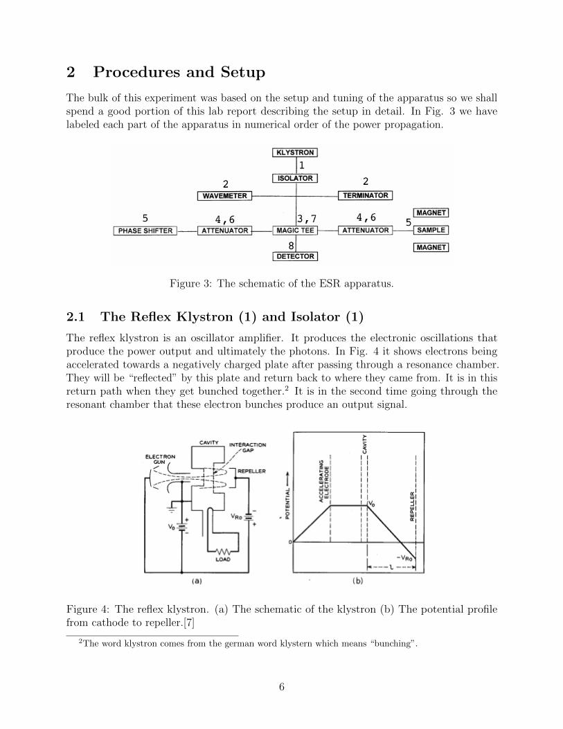
The reflex klystron is an oscillator amplifier. It produces the electronic oscillations thatproduce the power output and ultimately the photons. In Fig. 4 it shows electrons beingaccelerated towards a negatively charged plate after passing through a resonance chamber.They will be “reflected” by this plate and return back to where they came from. It is in thisreturn path when they get bunched together.2 It is in the second time going through theresonant chamber that these electron bunches produce an output signal.

Figure 4: The reflex klystron. (a) The schematic of the klystron (b) The potential profilefrom cathode to repeller.[7]

2The word klystron comes from the german word klystern which means “bunching”.

6

This signal also modulates the electrons velocity the first time they pass through theresonant chamber as well. The output signal gets picked up through charge accumulation onthe resonant chamber walls, this then gets transferred through to the load and pickup loop(the load and chamber circuit can be thought of equivalently as a voltage and current sourceand a LRC circuit.) By tuning the load (and it equivalent circuit) we get that a resonance ofthe circuit and hence the largest power output. The pickup loop is then sent to an antennawhich produces the microwave radiation.

Once the microwave radiation has been produced by the klystron, it is then passed throughthe isolator. The isolator is made from the chemical compound ferrite (of mainly iron oxidesi.e. Fe2O3). Ferrite along with a rotating magnetic field allow for the passing of the power inone direction but not in the reverse.

2.2 The Wave Meter (2) and Terminator (2)

The microwave frequency radiation then hits a “tee” which splits the power into two unequalparts. The small part gets diverted into the wave meter. This is a resonant cavity that willmeasure the frequency of the radiation and calibrate the klystron. It accomplishes this byfinely tuning the size the of the cavity to obtain maximum resonance which is picked up bythe crystal detector.

During the “tee” splitting some radiation gets split in the opposite direction of the wavemeter. This radiation is merely absorbed by material in the terminator to prevent it frominterfering with the main beam.

2.3 The Magic Tee (3,7)

The magic tee has four ports and output. The first two ports split the input (from klystron)into two equal beams. One goes toward the sample and one goes towards the phase shifter.On the return back to the tee the beams go into another port (one for each beam) and getdirected to the diode detector. The reason they don’t go back into the port they came fromis that there is an isolator type device that prevents back flow of power that would createinterference and attenuation of the signal. [3]

2.4 The Attenuator (4,6) and Phase Shifter (5)

The attenuator is essentially a piece of material that absorbs a small fraction of the photons.This device allows for essentially no reflection of signal. If signal were reflected it wouldcause significant signal attenuation and interference. Once the radiation passes through theattenuator it is reflected by the phase shifter. To change the phase of the radiation we justadjust the distance from the magic tee. For example if we adjusted the distance to be aquarter wavelength farther than the sample distance. Then the radiation would be half awavelength out of phase corresponding to half a wavelength farther in distance it has to travel(half wavelength is because extra quarter wavelength there and an extra quarter wavelengthback). We adjust these devices to make the signal down this arm equivalent to the signalcoming from the sample. This calibration makes the final signal maximum for resonance andessentially zero if we are off resonance. [3]

7

2.5 The Sample and Magnet (5)

After the beam is split at the magic tee, it heads to the sample (after first passing throughan attenuator). The smaple is in a rectangular wave guide, to direct the beam to the sampleefficiently. The sample as noted in the introduction is DPPH. We chose DPPH because ithas one free electron with no orbital angular momentum and it also has very diffuse unpairedspins which make the line widths very small. [1] The magnet is the standard Helmholtz coilswith some permanent magnets to confine the magnetic field to the inner region. For themagnetic fields we are probing we used a hall probe.

2.6 The Diode Detector (8)

The detector is a diode placed in the waveguide at the point of maximum electric field. [3]This electric field reduces the effective resistance of the diode and current begins to flow.The flow of current is then amplified even more and sent to the oscilloscope. The current isinversely proportional to the temperature squared and proportional to the radiation voltage,refer to the lab manual for more details[3]

3 Data and Analysis

We present our data, which is mainly in the form of oscilloscope plots. Some other data wasrecorded directly from the signal generators, magnetic field sources, and hall probe devicesand is summarized below.

3.1 The Wave Meter Q Factor

We measured the wave meter resonant frequency to be 9.256 GHz with a width of approxi-mately 50± 10 kHz. The quality factor is then

Q =ω

∆ω=

9.256 GHz

50.000 Hz= 1.8× 106 ± 0.2× 106 (7)

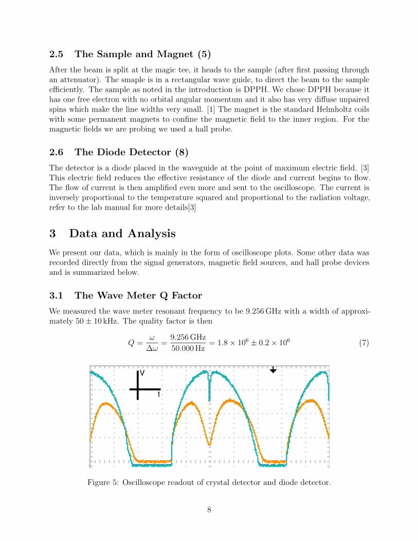
Figure 5: Oscilloscope readout of crystal detector and diode detector.

8

In Fig. 5 we observe the wave meter crystal detector signal (larger amplitude, blue) andthe diode detector signal (smaller amplitude, yellow). We expect the wave meter to have ahigher Q factor than the Q = 100 klystron resonant cavity. Comparing the two widths we seethat the klystron is indeed roughly 104 times wider than the wave meter Q (note the scaledifference).

3.2 Rectangular Wave Guide Cut Off Frequency Calculations

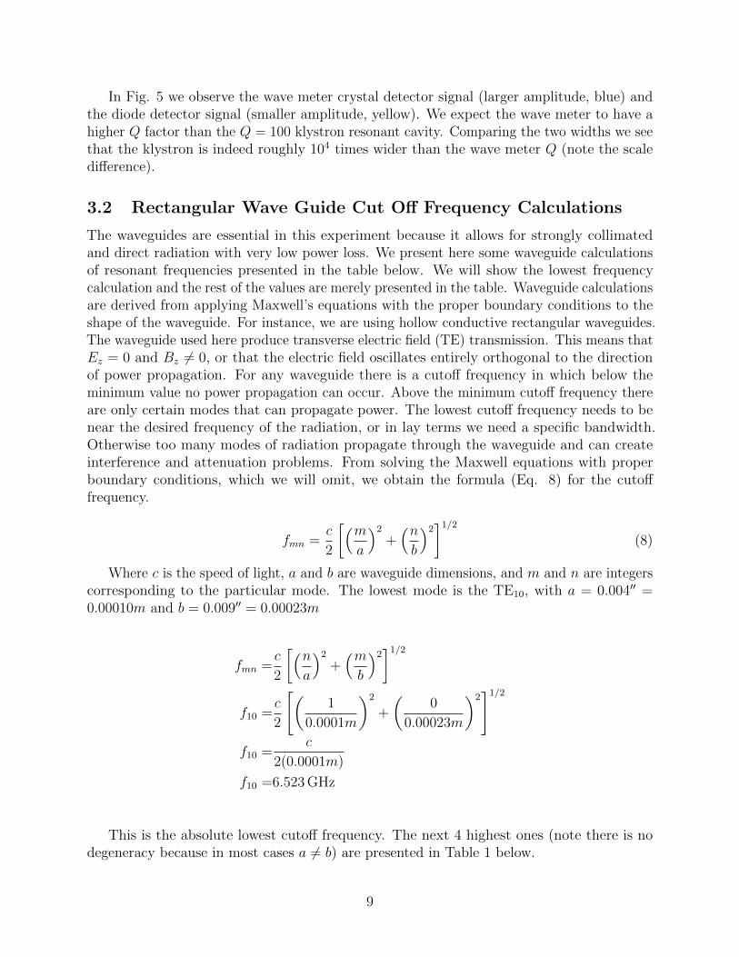
The waveguides are essential in this experiment because it allows for strongly collimatedand direct radiation with very low power loss. We present here some waveguide calculationsof resonant frequencies presented in the table below. We will show the lowest frequencycalculation and the rest of the values are merely presented in the table. Waveguide calculationsare derived from applying Maxwell’s equations with the proper boundary conditions to theshape of the waveguide. For instance, we are using hollow conductive rectangular waveguides.The waveguide used here produce transverse electric field (TE) transmission. This means thatEz = 0 and Bz 6= 0, or that the electric field oscillates entirely orthogonal to the directionof power propagation. For any waveguide there is a cutoff frequency in which below theminimum value no power propagation can occur. Above the minimum cutoff frequency thereare only certain modes that can propagate power. The lowest cutoff frequency needs to benear the desired frequency of the radiation, or in lay terms we need a specific bandwidth.Otherwise too many modes of radiation propagate through the waveguide and can createinterference and attenuation problems. From solving the Maxwell equations with properboundary conditions, which we will omit, we obtain the formula (Eq. 8) for the cutofffrequency.

fmn =c

2

[(ma

)2+(nb

)2]1/2(8)

Where c is the speed of light, a and b are waveguide dimensions, and m and n are integerscorresponding to the particular mode. The lowest mode is the TE10, with a = 0.004′′ =0.00010m and b = 0.009′′ = 0.00023m

fmn =c

2

[(na

)2+(mb

)2]1/2f10 =

c

2

[(1

0.0001m

)2

+

(0

0.00023m

)2]1/2

f10 =c

2(0.0001m)

f10 =6.523 GHz

This is the absolute lowest cutoff frequency. The next 4 highest ones (note there is nodegeneracy because in most cases a 6= b) are presented in Table 1 below.

9

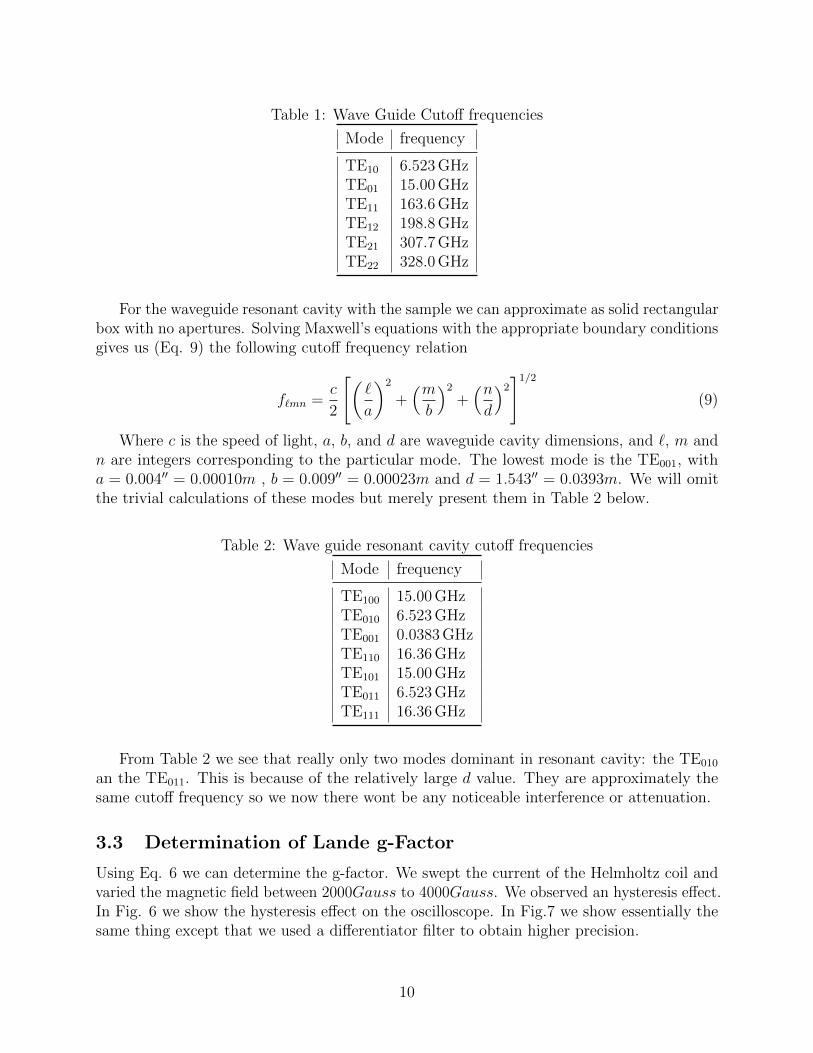
Table 1: Wave Guide Cutoff frequencies

Mode frequency

TE10 6.523 GHzTE01 15.00 GHzTE11 163.6 GHzTE12 198.8 GHzTE21 307.7 GHzTE22 328.0 GHz

For the waveguide resonant cavity with the sample we can approximate as solid rectangularbox with no apertures. Solving Maxwell’s equations with the appropriate boundary conditionsgives us (Eq. 9) the following cutoff frequency relation

f`mn =c

2

[(`

a

)2

+(mb

)2+(nd

)2]1/2(9)

Where c is the speed of light, a, b, and d are waveguide cavity dimensions, and `, m andn are integers corresponding to the particular mode. The lowest mode is the TE001, witha = 0.004′′ = 0.00010m , b = 0.009′′ = 0.00023m and d = 1.543′′ = 0.0393m. We will omitthe trivial calculations of these modes but merely present them in Table 2 below.

Table 2: Wave guide resonant cavity cutoff frequencies

Mode frequency

TE100 15.00 GHzTE010 6.523 GHzTE001 0.0383 GHzTE110 16.36 GHzTE101 15.00 GHzTE011 6.523 GHzTE111 16.36 GHz

From Table 2 we see that really only two modes dominant in resonant cavity: the TE010

an the TE011. This is because of the relatively large d value. They are approximately thesame cutoff frequency so we now there wont be any noticeable interference or attenuation.

3.3 Determination of Lande g-Factor

Using Eq. 6 we can determine the g-factor. We swept the current of the Helmholtz coil andvaried the magnetic field between 2000Gauss to 4000Gauss. We observed an hysteresis effect.In Fig. 6 we show the hysteresis effect on the oscilloscope. In Fig.7 we show essentially thesame thing except that we used a differentiator filter to obtain higher precision.

10

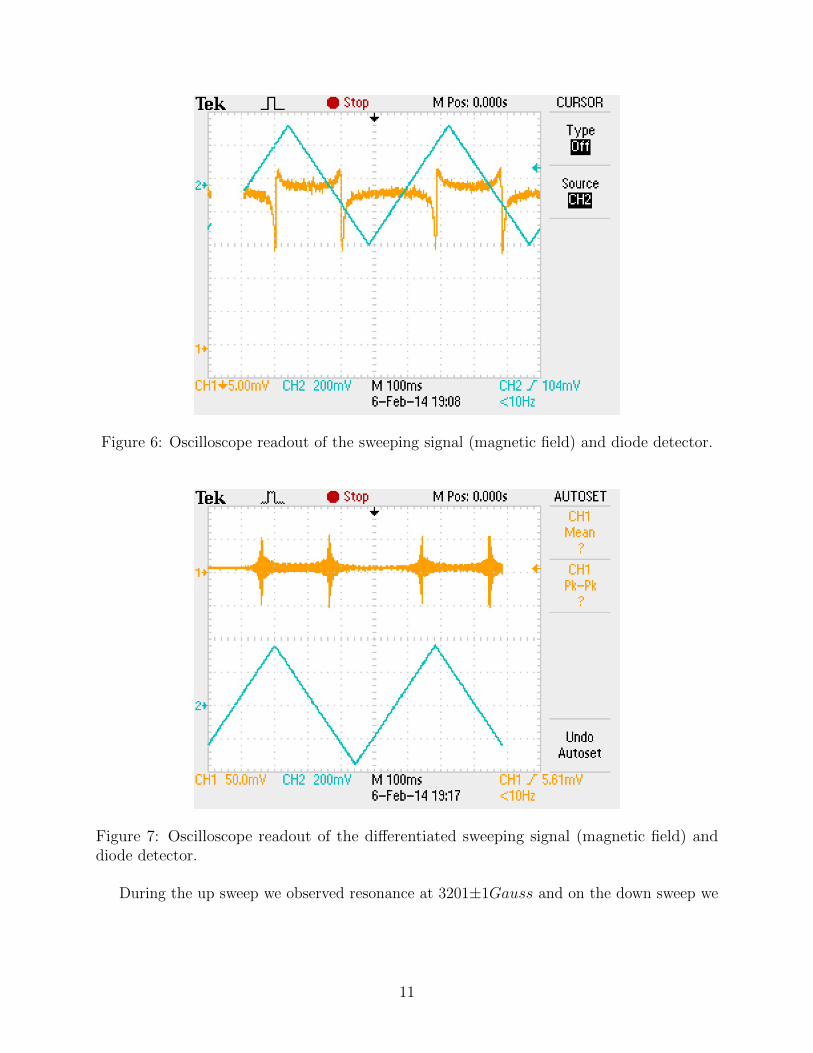
Figure 6: Oscilloscope readout of the sweeping signal (magnetic field) and diode detector.

Figure 7: Oscilloscope readout of the differentiated sweeping signal (magnetic field) anddiode detector.

During the up sweep we observed resonance at 3201±1Gauss and on the down sweep we

11

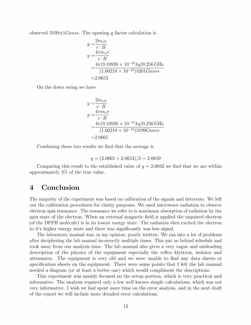
observed 3199±1Gauss. The upswing g factor calculation is

g =2meω

e−B

g =4πmeν

e−B

=4π(9.10938× 10−31kg)9.256 GHz

(1.60218× 10−19)3201Gauss

=2.0653

On the down swing we have

g =2meω

e−B

g =4πmeν

e−B

=4π(9.10938× 10−31kg)9.256 GHz

(1.60218× 10−19)3199Gauss

=2.0665

Combining these two results we find that the average is

g = (2.0665 + 2.0653)/2 = 2.0659

Comparing this result to the established value of g = 2.0032 we find that we are withinapproximately 3% of the true value.

4 Conclusion

The majority of the experiment was based on calibration of the signals and detectors. We leftout the calibration procedures for clarity purposes. We used microwave radiation to observeelectron spin resonance. The resonance we refer to is maximum absorption of radiation by thespin state of the electron. When an external magnetic field is applied the unpaired electron(of the DPPH molecule) is in its lowest energy state. The radiation then excited the electronto it’s higher energy state and there was significantly was less signal.

The laboratory manual was, in my opinion, poorly written. We ran into a lot of problemsafter deciphering the lab manual incorrectly multiple times. This put us behind schedule andtook away from our analysis time. The lab manual also gives a very vague and misleadingdescription of the physics of the equipment especially the reflex klystron, isolator andattenuator. The equipment is very old and we were unable to find any data sheets orspecification sheets on the equipment. There were some points that I felt the lab manualneeded a diagram (or at least a better one) which would compliment the descriptions.

This experiment was mainly focused on the setup portion, which is very practical andinformative. The analysis required only a few well known simple calculations, which was notvery informative. I wish we had spent more time on the error analysis, and in the next draftof the report we will include more detailed error calculations.

12

References

[1] Dunn, E.K. ESR of DPPH, 2011. University of Kansas.

[2] https://physics.ucsd.edu/students/courses/spring2012/physics4e/zeemaneffect.pdf

[3] George Brown, Sue Carter. Physics 134 Lab Manual. Winter 2014.

[4] http://plato.stanford.edu/entries/physics-experiment/app5.html. Stanford Encyclope-dia.

[5] http://www.lorentz.leidenuniv.nl/history/spin/goudsmit.html

[6] Weil, John and Bolton, James. Electron Paramagnetic Resonance. 2007.

[7] Principles of Electron Tubes, Including Grid-Controlled Tubes, Microwave Tubes andGas Tubes. J. W. Gewartowski and H. A. Watson. Bell Telephone Laboratories 1965

13