Electromagnetic Field Theory - irina.stobbe.netirina.stobbe.net/wiki/images/EMFT_Book.pdf ·...
223
Electromagnetic Field Theory B O T HIDÉ ϒ UPSILON B OOKS
Transcript of Electromagnetic Field Theory - irina.stobbe.netirina.stobbe.net/wiki/images/EMFT_Book.pdf ·...
ElectromagneticField Theory
BO THIDÉ
ϒUPSILON BOOKS

ELECTROMAGNETIC FIELD THEORY

ElectromagneticField Theory
BO THIDÉ
Swedish Institute of Space PhysicsUppsala, Sweden
and
Department of Astronomy and Space PhysicsUppsala University, Sweden
and
LOIS Space CentreSchool of Mathematics and Systems Engineering
Växjö University, Sweden
ϒ
UPSILON BOOKS · UPPSALA · SWEDEN
Also available
ELECTROMAGNETIC FIELD THEORY
EXERCISES
byTobia Carozzi, Anders Eriksson, Bengt Lundborg,
Bo Thidé and Mattias Waldenvik
Freely downloadable fromwww.plasma.uu.se/CED
This book was typeset in LATEX 2ε (based on TEX 3.141592 and Web2C 7.4.4) on an HP Visu-alize 9000⁄3600 workstation running HP-UX 11.11.
Copyright©1997–2006 byBo ThidéUppsala, SwedenAll rights reserved.
Electromagnetic Field TheoryISBN X-XXX-XXXXX-X
To the memory of professorLEV MIKHAILOVICH ERUKHIMOV (1936–1997)
dear friend, great physicist, poetand a truly remarkable man.

Downloaded from http://www.plasma.uu.se/CED/Book Version released 29th September 2007 at 21:55.
Contents
Contents ix
List of Figures xiii
Preface xv
1 Classical Electrodynamics 11.1 Electrostatics 2
1.1.1 Coulomb’s law 21.1.2 The electrostatic field 3
1.2 Magnetostatics 61.2.1 Ampère’s law 61.2.2 The magnetostatic field 7
1.3 Electrodynamics 91.3.1 Equation of continuity for electric charge 101.3.2 Maxwell’s displacement current 101.3.3 Electromotive force 111.3.4 Faraday’s law of induction 121.3.5 Maxwell’s microscopic equations 151.3.6 Maxwell’s macroscopic equations 15
1.4 Electromagnetic duality 161.5 Bibliography 181.6 Examples 21
2 Electromagnetic Waves 272.1 The wave equations 28
2.1.1 The wave equation for E 282.1.2 The wave equation for B 292.1.3 The time-independent wave equation for E 29
ix
Contents
2.2 Plane waves 322.2.1 Telegrapher’s equation 332.2.2 Waves in conductive media 34
2.3 Observables and averages 352.4 Bibliography 362.5 Example 40
3 Electromagnetic Potentials 433.1 The electrostatic scalar potential 433.2 The magnetostatic vector potential 443.3 The electrodynamic potentials 443.4 Gauge transformations 453.5 Gauge conditions 46
3.5.1 Lorenz-Lorentz gauge 473.5.2 Coulomb gauge 513.5.3 Velocity gauge 53
3.6 Bibliography 533.7 Examples 55
4 Electromagnetic Fields and Matter 574.1 Electric polarisation and displacement 57
4.1.1 Electric multipole moments 574.2 Magnetisation and the magnetising field 604.3 Energy and momentum 62
4.3.1 The energy theorem in Maxwell’s theory 624.3.2 The momentum theorem in Maxwell’s theory 63
4.4 Bibliography 664.5 Example 67
5 Electromagnetic Fields from Arbitrary Source Distributions 695.1 The magnetic field 715.2 The electric field 735.3 The radiation fields 755.4 Radiated energy 78
5.4.1 Monochromatic signals 785.4.2 Finite bandwidth signals 79
5.5 Bibliography 80
6 Electromagnetic Radiation and Radiating Systems 816.1 Radiation from an extended source volume at rest 81
6.1.1 Radiation from a one-dimensional current distribution 82
x Version released 29th September 2007 at 21:55. Downloaded from http://www.plasma.uu.se/CED/Book
6.1.2 Radiation from a two-dimensional current distribution 856.2 Radiation from a localised source volume at rest 89
6.2.1 The Hertz potential 896.2.2 Electric dipole radiation 936.2.3 Magnetic dipole radiation 956.2.4 Electric quadrupole radiation 96
6.3 Radiation from a localised charge in arbitrary motion 976.3.1 The Liénard-Wiechert potentials 986.3.2 Radiation from an accelerated point charge 1006.3.3 Bremsstrahlung 1086.3.4 Cyclotron and synchrotron radiation 1126.3.5 Radiation from charges moving in matter 119
6.4 Bibliography 1266.5 Examples 128
7 Relativistic Electrodynamics 1357.1 The special theory of relativity 135
7.1.1 The Lorentz transformation 1367.1.2 Lorentz space 1387.1.3 Minkowski space 143
7.2 Covariant classical mechanics 1467.3 Covariant classical electrodynamics 147
7.3.1 The four-potential 1477.3.2 The Liénard-Wiechert potentials 1487.3.3 The electromagnetic field tensor 151
7.4 Bibliography 154
8 Electromagnetic Fields and Particles 1578.1 Charged particles in an electromagnetic field 157
8.1.1 Covariant equations of motion 1578.2 Covariant field theory 163
8.2.1 Lagrange-Hamilton formalism for fields and interactions 1648.3 Bibliography 1718.4 Example 173
F Formulæ 175F.1 The electromagnetic field 175
F.1.1 Maxwell’s equations 175F.1.2 Fields and potentials 175F.1.3 Force and energy 176
F.2 Electromagnetic radiation 176
Downloaded from http://www.plasma.uu.se/CED/Book Version released 29th September 2007 at 21:55. xi
Contents
F.2.1 Relationship between the field vectors in a plane wave 176F.2.2 The far fields from an extended source distribution 176F.2.3 The far fields from an electric dipole 176F.2.4 The far fields from a magnetic dipole 177F.2.5 The far fields from an electric quadrupole 177F.2.6 The fields from a point charge in arbitrary motion 177
F.3 Special relativity 178F.3.1 Metric tensor 178F.3.2 Covariant and contravariant four-vectors 178F.3.3 Lorentz transformation of a four-vector 178F.3.4 Invariant line element 178F.3.5 Four-velocity 178F.3.6 Four-momentum 179F.3.7 Four-current density 179F.3.8 Four-potential 179F.3.9 Field tensor 179
F.4 Vector relations 179F.4.1 Spherical polar coordinates 180F.4.2 Vector formulae 180
F.5 Bibliography 182
M Mathematical Methods 183M.1 Scalars, vectors and tensors 183
M.1.1 Vectors 183M.1.2 Fields 185M.1.3 Vector algebra 188M.1.4 Vector analysis 190
M.2 Analytical mechanics 192M.2.1 Lagrange’s equations 192M.2.2 Hamilton’s equations 193
M.3 Examples 194M.4 Bibliography 202
Index 203
xii Version released 29th September 2007 at 21:55. Downloaded from http://www.plasma.uu.se/CED/Book
Downloaded from http://www.plasma.uu.se/CED/Book Version released 29th September 2007 at 21:55.
List of Figures
1.1 Coulomb interaction between two electric charges 31.2 Coulomb interaction for a distribution of electric charges 51.3 Ampère interaction 71.4 Moving loop in a varying B field 13
5.1 Radiation in the far zone 77
6.1 Linear antenna 836.2 Electric dipole antenna geometry 846.3 Loop antenna 866.4 Multipole radiation geometry 916.5 Electric dipole geometry 936.6 Radiation from a moving charge in vacuum 986.7 An accelerated charge in vacuum 1006.8 Angular distribution of radiation during bremsstrahlung 1096.9 Location of radiation during bremsstrahlung 1106.10 Radiation from a charge in circular motion 1136.11 Synchrotron radiation lobe width 1156.12 The perpendicular field of a moving charge 1176.13 Electron-electron scattering 1196.14 Vavilov-Cerenkov cone 124
7.1 Relative motion of two inertial systems 1377.2 Rotation in a 2D Euclidean space 1437.3 Minkowski diagram 144
8.1 Linear one-dimensional mass chain 164
M.1 Tetrahedron-like volume element of matter 194
xiii

Downloaded from http://www.plasma.uu.se/CED/Book Version released 29th September 2007 at 21:55.
Preface
This book is the result of a more than thirty year long love affair. In 1972, I tookmy first advanced course in electrodynamics at the Department of TheoreticalPhysics, Uppsala University. A year later, I joined the research group there andtook on the task of helping professor PER OLOF FRÖMAN, who later become myPh.D. thesis advisor, with the preparation of a new version of his lecture notes onthe Theory of Electricity. These two things opened up my eyes for the beauty andintricacy of electrodynamics, already at the classical level, and I fell in love withit. Ever since that time, I have on and off had reason to return to electrodynamics,both in my studies, research and the teaching of a course in advanced electrody-namics at Uppsala University some twenty odd years after I experienced the firstencounter with this subject.
The current version of the book is an outgrowth of the lecture notes that I pre-pared for the four-credit course Electrodynamics that was introduced in the Up-psala University curriculum in 1992, to become the five-credit course ClassicalElectrodynamics in 1997. To some extent, parts of these notes were based on lec-ture notes prepared, in Swedish, by my friend and colleague BENGT LUNDBORG,who created, developed and taught the earlier, two-credit course ElectromagneticRadiation at our faculty.
Intended primarily as a textbook for physics students at the advanced under-graduate or beginning graduate level, it is hoped that the present book may beuseful for research workers too. It provides a thorough treatment of the theoryof electrodynamics, mainly from a classical field theoretical point of view, andincludes such things as formal electrostatics and magnetostatics and their uni-fication into electrodynamics, the electromagnetic potentials, gauge transforma-tions, covariant formulation of classical electrodynamics, force, momentum andenergy of the electromagnetic field, radiation and scattering phenomena, electro-magnetic waves and their propagation in vacuum and in media, and covariantLagrangian/Hamiltonian field theoretical methods for electromagnetic fields, par-ticles and interactions. The aim has been to write a book that can serve both asan advanced text in Classical Electrodynamics and as a preparation for studies inQuantum Electrodynamics and related subjects.
In an attempt to encourage participation by other scientists and students inthe authoring of this book, and to ensure its quality and scope to make it useful
xv
Preface
in higher university education anywhere in the world, it was produced within aWorld-Wide Web (WWW) project. This turned out to be a rather successful move.By making an electronic version of the book freely down-loadable on the net,comments have been received from fellow Internet physicists around the worldand from WWW ‘hit’ statistics it seems that the book serves as a frequently usedInternet resource.1 This way it is hoped that it will be particularly useful forstudents and researchers working under financial or other circumstances that makeit difficult to procure a printed copy of the book.
Thanks are due not only to Bengt Lundborg for providing the inspiration towrite this book, but also to professor CHRISTER WAHLBERG and professor GÖRAN
FÄLDT, Uppsala University, and professor YAKOV ISTOMIN, Lebedev Institute,Moscow, for interesting discussions on electrodynamics and relativity in generaland on this book in particular. Comments from former graduate students MATTIAS
WALDENVIK, TOBIA CAROZZI and ROGER KARLSSON as well as ANDERS ERIKS-SON, all at the Swedish Institute of Space Physics in Uppsala and who all haveparticipated in the teaching on the material covered in the course and in this bookare gratefully acknowledged. Thanks are also due to my long-term space physicscolleague HELMUT KOPKA of the Max-Planck-Institut für Aeronomie, Lindau,Germany, who not only taught me about the practical aspects of high-power radiowave transmitters and transmission lines, but also about the more delicate aspectsof typesetting a book in TEX and LATEX. I am particularly indebted to Academicianprofessor VITALIY LAZAREVICH GINZBURG, 2003 Nobel Laureate in Physics, forhis many fascinating and very elucidating lectures, comments and historical noteson electromagnetic radiation and cosmic electrodynamics while cruising on theVolga river at our joint Russian-Swedish summer schools during the 1990s, andfor numerous private discussions over the years.
Finally, I would like to thank all students and Internet users who have down-loaded and commented on the book during its life on the World-Wide Web.
I dedicate this book to my son MATTIAS, my daughter KAROLINA, myhigh-school physics teacher, STAFFAN RÖSBY, and to my fellow members of theCAPELLA PEDAGOGICA UPSALIENSIS.
Uppsala, Sweden BO THIDÉ
December, 2006 www.physics.irfu.se/∼bt
1At the time of publication of this edition, more than 500 000 downloads have been recorded.
xvi Version released 29th September 2007 at 21:55. Downloaded from http://www.plasma.uu.se/CED/Book
Downloaded from http://www.plasma.uu.se/CED/Book Version released 29th September 2007 at 21:55.
1Classical
Electrodynamics
Classical electrodynamics deals with electric and magnetic fields and interactionscaused by macroscopic distributions of electric charges and currents. This meansthat the concepts of localised electric charges and currents assume the validity ofcertain mathematical limiting processes in which it is considered possible for thecharge and current distributions to be localised in infinitesimally small volumes ofspace. Clearly, this is in contradiction to electromagnetism on a truly microscopicscale, where charges and currents have to be treated as spatially extended objectsand quantum corrections must be included. However, the limiting processes usedwill yield results which are correct on small as well as large macroscopic scales.
It took the genius of JAMES CLERK MAXWELL to unify electricity and mag-netism into a super-theory, electromagnetism or classical electrodynamics (CED),and to realise that optics is a subfield of this super-theory. Early in the 20th cen-tury, HENDRIK ANTOON LORENTZ took the electrodynamics theory further to themicroscopic scale and also laid the foundation for the special theory of relativity,formulated by ALBERT EINSTEIN in 1905. In the 1930s PAUL A. M. DIRAC ex-panded electrodynamics to a more symmetric form, including magnetic as wellas electric charges. With his relativistic quantum mechanics, he also paved theway for the development of quantum electrodynamics (QED) for which RICHARD
P. FEYNMAN, JULIAN SCHWINGER, and SIN-ITIRO TOMONAGA in 1965 receivedtheir Nobel prizes in physics. Around the same time, physicists such as SHELDON
GLASHOW, ABDUS SALAM, and STEVEN WEINBERG were able to unify electro-dynamics the weak interaction theory to yet another super-theory, electroweaktheory, an achievement which rendered them the Nobel prize in physics 1979.The modern theory of strong interactions, quantum chromodynamics (QCD), isinfluenced by QED.
In this chapter we start with the force interactions in classical electrostatics
1
1. Classical Electrodynamics
and classical magnetostatics and introduce the static electric and magnetic fieldsto find two uncoupled systems of equations for them. Then we see how the con-servation of electric charge and its relation to electric current leads to the dynamicconnection between electricity and magnetism and how the two can be unifiedinto one ‘super-theory’, classical electrodynamics, described by one system ofeight coupled dynamic field equations—the Maxwell equations.
At the end of this chapter we study Dirac’s symmetrised form of Maxwell’sequations by introducing (hypothetical) magnetic charges and magnetic currentsinto the theory. While not identified unambiguously in experiments yet, mag-netic charges and currents make the theory much more appealing, for instance byallowing for duality transformations in a most natural way.
1.1 ElectrostaticsThe theory which describes physical phenomena related to the interaction be-tween stationary electric charges or charge distributions in a finite space whichhas stationary boundaries is called electrostatics. For a long time, electrostatics,under the name electricity, was considered an independent physical theory of itsown, alongside other physical theories such as magnetism, mechanics, optics andthermodynamics.1
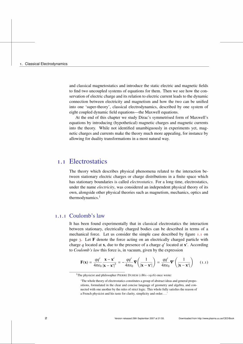
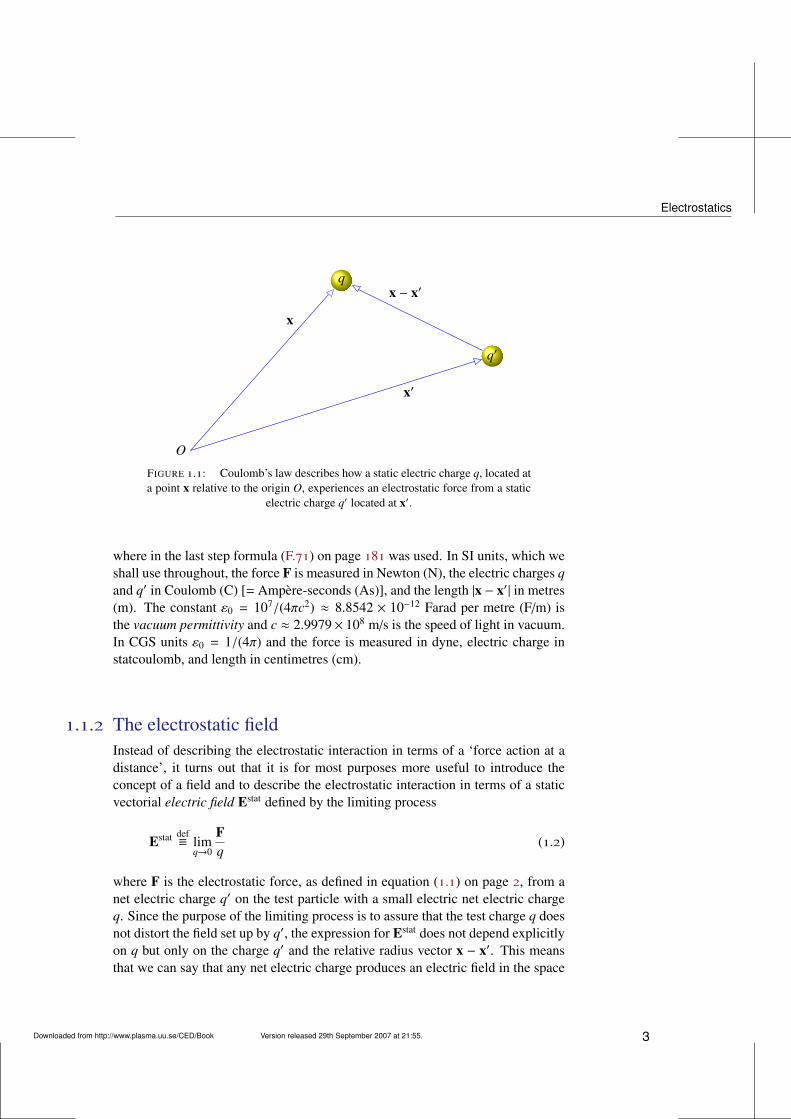
1.1.1 Coulomb’s lawIt has been found experimentally that in classical electrostatics the interactionbetween stationary, electrically charged bodies can be described in terms of amechanical force. Let us consider the simple case described by figure 1.1 onpage 3. Let F denote the force acting on an electrically charged particle withcharge q located at x, due to the presence of a charge q′ located at x′. Accordingto Coulomb’s law this force is, in vacuum, given by the expression
F(x) =qq′
4πε0
x − x′
|x − x′|3= −
qq′
4πε0∇
(1
|x − x′|
)=
qq′
4πε0∇′
(1
|x − x′|
)(1.1)
1The physicist and philosopher PIERRE DUHEM (1861–1916) once wrote:
‘The whole theory of electrostatics constitutes a group of abstract ideas and general propo-sitions, formulated in the clear and concise language of geometry and algebra, and con-nected with one another by the rules of strict logic. This whole fully satisfies the reason ofa French physicist and his taste for clarity, simplicity and order. . . .’
2 Version released 29th September 2007 at 21:55. Downloaded from http://www.plasma.uu.se/CED/Book
Electrostatics
q′
q
O
x′
x − x′
x
FIGURE 1.1: Coulomb’s law describes how a static electric charge q, located ata point x relative to the origin O, experiences an electrostatic force from a static
electric charge q′ located at x′.
where in the last step formula (F.71) on page 181 was used. In SI units, which weshall use throughout, the force F is measured in Newton (N), the electric charges qand q′ in Coulomb (C) [= Ampère-seconds (As)], and the length |x − x′| in metres(m). The constant ε0 = 107/(4πc2) ≈ 8.8542 × 10⁻¹² Farad per metre (F/m) isthe vacuum permittivity and c ≈ 2.9979× 10⁸ m/s is the speed of light in vacuum.In CGS units ε0 = 1/(4π) and the force is measured in dyne, electric charge instatcoulomb, and length in centimetres (cm).
1.1.2 The electrostatic fieldInstead of describing the electrostatic interaction in terms of a ‘force action at adistance’, it turns out that it is for most purposes more useful to introduce theconcept of a field and to describe the electrostatic interaction in terms of a staticvectorial electric field Estat defined by the limiting process
Estat def≡ lim
q→0
Fq
(1.2)
where F is the electrostatic force, as defined in equation (1.1) on page 2, from anet electric charge q′ on the test particle with a small electric net electric chargeq. Since the purpose of the limiting process is to assure that the test charge q doesnot distort the field set up by q′, the expression for Estat does not depend explicitlyon q but only on the charge q′ and the relative radius vector x − x′. This meansthat we can say that any net electric charge produces an electric field in the space
Downloaded from http://www.plasma.uu.se/CED/Book Version released 29th September 2007 at 21:55. 3
1. Classical Electrodynamics
that surrounds it, regardless of the existence of a second charge anywhere in thisspace.2
Using (1.1) and equation (1.2) on page 3, and formula (F.70) on page 181,we find that the electrostatic field Estat at the field point x (also known as theobservation point), due to a field-producing electric charge q′ at the source pointx′, is given by
Estat(x) =q′
4πε0
x − x′
|x − x′|3= −
q′
4πε0∇
(1
|x − x′|
)=
q′
4πε0∇′
(1
|x − x′|
)(1.3)
In the presence of several field producing discrete electric charges q′i , locatedat the points x′i , i = 1, 2, 3, . . . , respectively, in an otherwise empty space, the as-sumption of linearity of vacuum3 allows us to superimpose their individual elec-trostatic fields into a total electrostatic field
Estat(x) =1
4πε0∑
iq′i
x − x′i∣∣x − x′i∣∣3 (1.4)
If the discrete electric charges are small and numerous enough, we introducethe electric charge density ρ, measured in C/m3 in SI units, located at x′ withina volume V ′ of limited extent and replace summation with integration over thisvolume. This allows us to describe the total field as
Estat(x) =1
4πε0
∫V ′
d3x′ ρ(x′)x − x′
|x − x′|3= −
14πε0
∫V ′
d3x′ ρ(x′)∇(
1|x − x′|
)= −
14πε0
∇
∫V ′
d3x′ρ(x′)|x − x′|
(1.5)
where we used formula (F.70) on page 181 and the fact that ρ(x′) does not dependon the unprimed (field point) coordinates on which ∇ operates.
2In the preface to the first edition of the first volume of his book A Treatise on Electricity and Mag-netism, first published in 1873, James Clerk Maxwell describes this in the following almost poetic manner[26]:
‘For instance, Faraday, in his mind’s eye, saw lines of force traversing all space where themathematicians saw centres of force attracting at a distance: Faraday saw a medium wherethey saw nothing but distance: Faraday sought the seat of the phenomena in real actionsgoing on in the medium, they were satisfied that they had found it in a power of action ata distance impressed on the electric fluids.’
3In fact, vacuum exhibits a quantum mechanical nonlinearity due to vacuum polarisation effects man-ifesting themselves in the momentary creation and annihilation of electron-positron pairs, but classicallythis nonlinearity is negligible.
4 Version released 29th September 2007 at 21:55. Downloaded from http://www.plasma.uu.se/CED/Book
Electrostatics
V ′
q′i
q
O
x′i
x − x′i
x
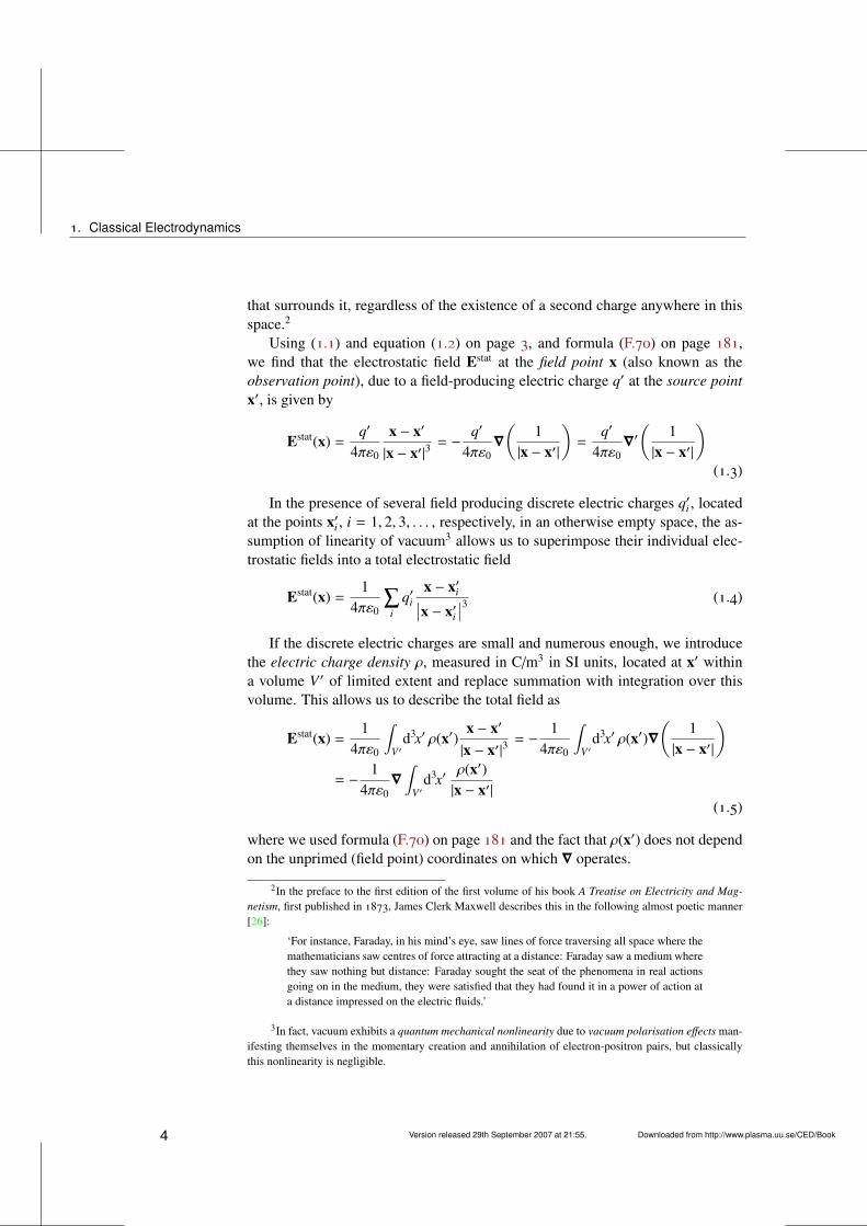
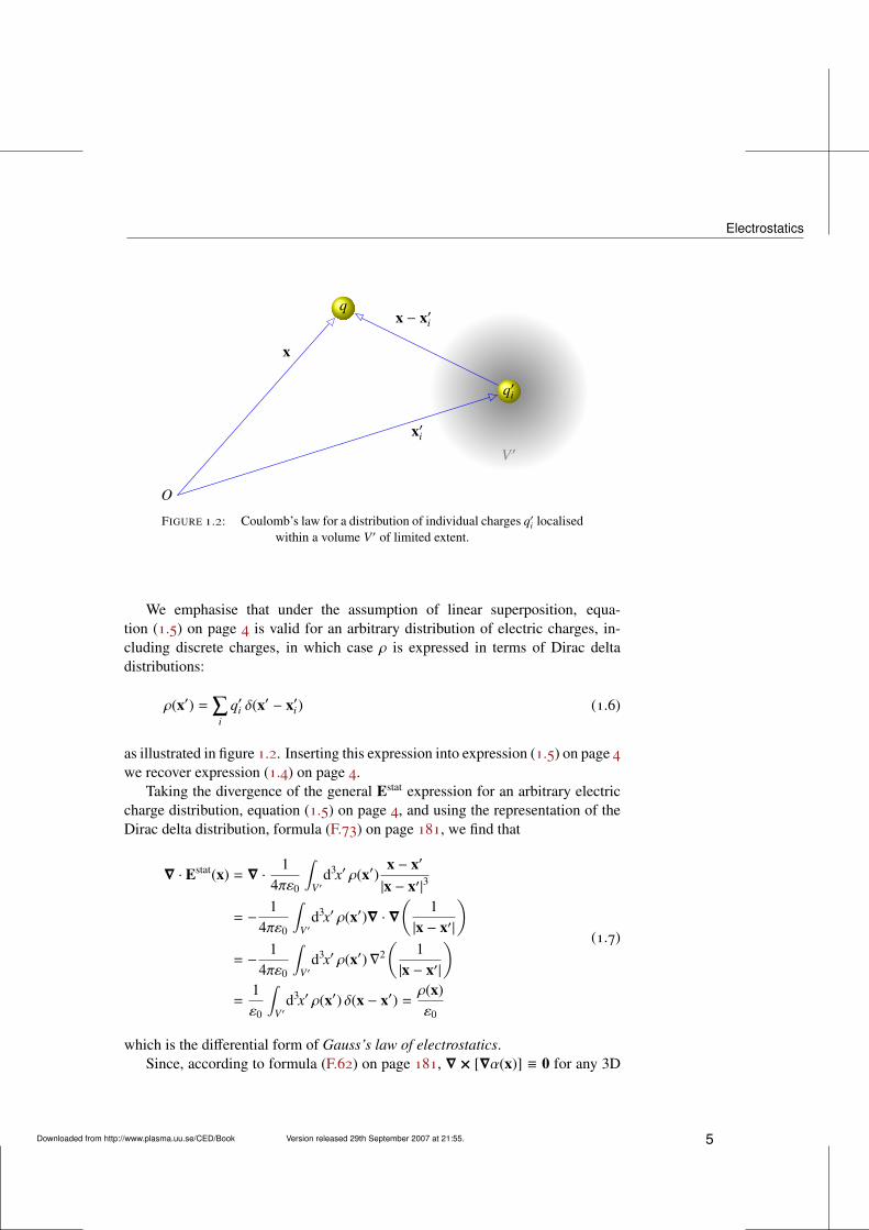
FIGURE 1.2: Coulomb’s law for a distribution of individual charges q′i localisedwithin a volume V ′ of limited extent.
We emphasise that under the assumption of linear superposition, equa-tion (1.5) on page 4 is valid for an arbitrary distribution of electric charges, in-cluding discrete charges, in which case ρ is expressed in terms of Dirac deltadistributions:
ρ(x′) =∑i
q′i δ(x′ − x′i) (1.6)
as illustrated in figure 1.2. Inserting this expression into expression (1.5) on page 4we recover expression (1.4) on page 4.
Taking the divergence of the general Estat expression for an arbitrary electriccharge distribution, equation (1.5) on page 4, and using the representation of theDirac delta distribution, formula (F.73) on page 181, we find that
∇ · Estat(x) = ∇ ·1
4πε0
∫V ′
d3x′ ρ(x′)x − x′
|x − x′|3
= −1
4πε0
∫V ′
d3x′ ρ(x′)∇ · ∇(
1|x − x′|
)= −
14πε0
∫V ′
d3x′ ρ(x′)∇2(
1|x − x′|
)=
1ε0
∫V ′
d3x′ ρ(x′) δ(x − x′) =ρ(x)ε0
(1.7)
which is the differential form of Gauss’s law of electrostatics.Since, according to formula (F.62) on page 181, ∇ × [∇α(x)] ≡ 0 for any 3D
Downloaded from http://www.plasma.uu.se/CED/Book Version released 29th September 2007 at 21:55. 5
1. Classical Electrodynamics
R3 scalar field α(x), we immediately find that in electrostatics
∇ × Estat(x) = −1
4πε0∇ ×
(∇
∫V ′
d3x′ρ(x′)|x − x′|
)= 0 (1.8)
i.e., that Estat is an irrotational field.To summarise, electrostatics can be described in terms of two vector partial
differential equations
∇ · Estat(x) =ρ(x)ε0
(1.9a)
∇ × Estat(x) = 0 (1.9b)
representing four scalar partial differential equations.
1.2 MagnetostaticsWhile electrostatics deals with static electric charges, magnetostatics deals withstationary electric currents, i.e., electric charges moving with constant speeds, andthe interaction between these currents. Here we shall discuss this theory in somedetail.
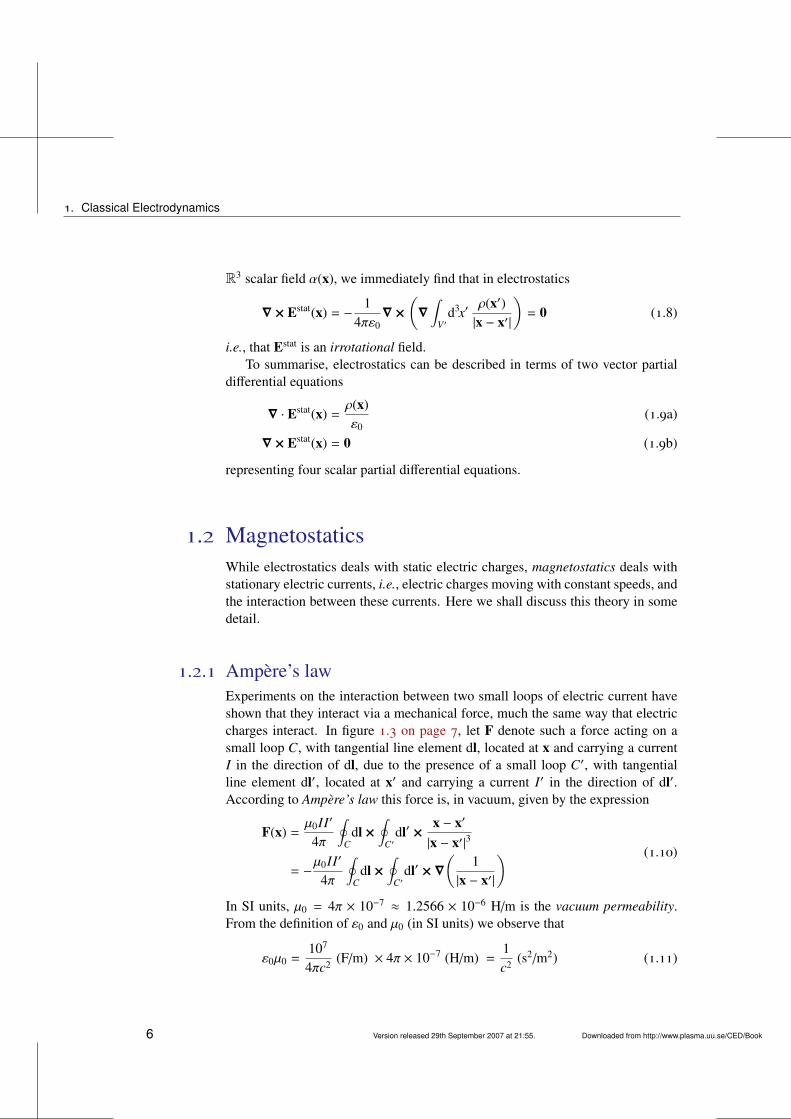
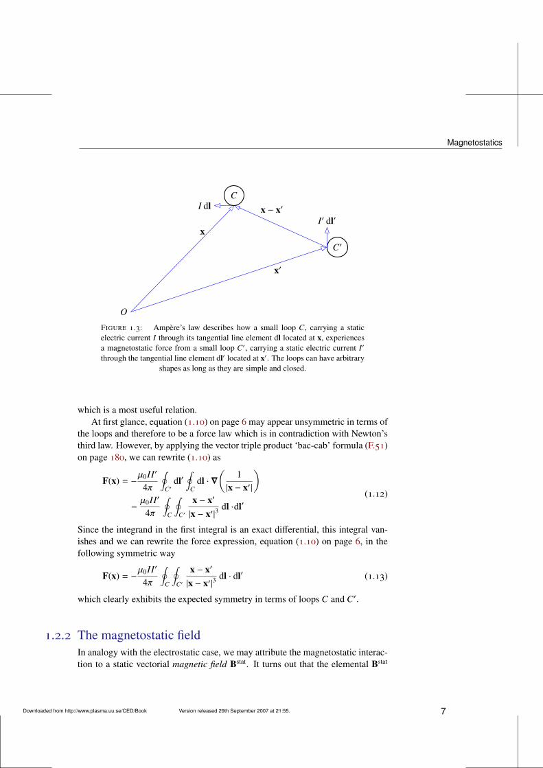
1.2.1 Ampère’s lawExperiments on the interaction between two small loops of electric current haveshown that they interact via a mechanical force, much the same way that electriccharges interact. In figure 1.3 on page 7, let F denote such a force acting on asmall loop C, with tangential line element dl, located at x and carrying a currentI in the direction of dl, due to the presence of a small loop C′, with tangentialline element dl′, located at x′ and carrying a current I′ in the direction of dl′.According to Ampère’s law this force is, in vacuum, given by the expression
F(x) =µ0II′
4π
∮C
dl ×∮
C′dl′ ×
x − x′
|x − x′|3
= −µ0II′
4π
∮C
dl ×∮
C′dl′ × ∇
(1
|x − x′|
) (1.10)
In SI units, µ0 = 4π × 10−7 ≈ 1.2566 × 10⁻⁶ H/m is the vacuum permeability.From the definition of ε0 and µ0 (in SI units) we observe that
ε0µ0 =107
4πc2 (F/m) × 4π × 10−7 (H/m) =1c2 (s2/m2) (1.11)
6 Version released 29th September 2007 at 21:55. Downloaded from http://www.plasma.uu.se/CED/Book
Magnetostatics
C′
C
I′ dl′I dl
O
x′
x − x′
x
FIGURE 1.3: Ampère’s law describes how a small loop C, carrying a staticelectric current I through its tangential line element dl located at x, experiencesa magnetostatic force from a small loop C′, carrying a static electric current I′
through the tangential line element dl′ located at x′. The loops can have arbitraryshapes as long as they are simple and closed.
which is a most useful relation.At first glance, equation (1.10) on page 6may appear unsymmetric in terms of
the loops and therefore to be a force law which is in contradiction with Newton’sthird law. However, by applying the vector triple product ‘bac-cab’ formula (F.51)on page 180, we can rewrite (1.10) as
F(x) = −µ0II′
4π
∮C′
dl′∮
Cdl · ∇
(1
|x − x′|
)−µ0II′
4π
∮C
∮C′
x − x′
|x − x′|3dl ·dl′
(1.12)
Since the integrand in the first integral is an exact differential, this integral van-ishes and we can rewrite the force expression, equation (1.10) on page 6, in thefollowing symmetric way
F(x) = −µ0II′
4π
∮C
∮C′
x − x′
|x − x′|3dl · dl′ (1.13)
which clearly exhibits the expected symmetry in terms of loops C and C′.
1.2.2 The magnetostatic fieldIn analogy with the electrostatic case, we may attribute the magnetostatic interac-tion to a static vectorial magnetic field Bstat. It turns out that the elemental Bstat
Downloaded from http://www.plasma.uu.se/CED/Book Version released 29th September 2007 at 21:55. 7
1. Classical Electrodynamics
can be defined as
dBstat(x)def≡µ0I′
4πdl′ ×
x − x′
|x − x′|3(1.14)
which expresses the small element dBstat(x) of the static magnetic field set up atthe field point x by a small line element dl′ of stationary current I′ at the sourcepoint x′. The SI unit for the magnetic field, sometimes called the magnetic fluxdensity or magnetic induction, is Tesla (T).
If we generalise expression (1.14) to an integrated steady state electric currentdensity j(x), measured in A/m2 in SI units, we obtain Biot-Savart’s law:
Bstat(x) =µ0
4π
∫V ′
d3x′ j(x′) ×x − x′
|x − x′|3= −
µ0
4π
∫V ′
d3x′ j(x′) × ∇(
1|x − x′|
)=µ0
4π∇ ×
∫V ′
d3x′j(x′)|x − x′|
(1.15)
where we used formula (F.70) on page 181, formula (F.57) on page 181, and thefact that j(x′) does not depend on the unprimed coordinates on which ∇ operates.Comparing equation (1.5) on page 4 with equation (1.15), we see that there existsa close analogy between the expressions for Estat and Bstat but that they differin their vectorial characteristics. With this definition of Bstat, equation (1.10) onpage 6 may we written
F(x) = I∮
Cdl × Bstat(x) (1.16)
In order to assess the properties of Bstat, we determine its divergence and curl.Taking the divergence of both sides of equation (1.15) and utilising formula (F.63)on page 181, we obtain
∇ · Bstat(x) =µ0
4π∇ ·
(∇ ×
∫V ′
d3x′j(x′)|x − x′|
)= 0 (1.17)
since, according to formula (F.63) on page 181, ∇ · (∇×a) vanishes for any vectorfield a(x).
Applying the operator ‘bac-cab’ rule, formula (F.64) on page 181, the curl ofequation (1.15) can be written
∇ × Bstat(x) =µ0
4π∇ ×
(∇ ×
∫V ′
d3x′j(x′)|x − x′|
)=
= −µ0
4π
∫V ′
d3x′ j(x′)∇2(
1|x − x′|
)+µ0
4π
∫V ′
d3x′ [j(x′) · ∇′]∇′(
1|x − x′|
)(1.18)
8 Version released 29th September 2007 at 21:55. Downloaded from http://www.plasma.uu.se/CED/Book
Electrodynamics
In the first of the two integrals on the right-hand side, we use the representationof the Dirac delta function given in formula (F.73) on page 181, and integrate thesecond one by parts, by utilising formula (F.56) on page 181 as follows:∫
V ′d3x′ [j(x′) · ∇′]∇′
(1
|x − x′|
)= xk
∫V ′
d3x′∇′ ·
j(x′)[∂
∂x′k
(1
|x − x′|
)]−
∫V ′
d3x′[∇′ · j(x′)
]∇′
(1
|x − x′|
)= xk
∫S ′
d2x′ n′ · j(x′)∂
∂x′k
(1
|x − x′|
)−
∫V ′
d3x′[∇′ · j(x′)
]∇′
(1
|x − x′|
)(1.19)
Then we note that the first integral in the result, obtained by applying Gauss’stheorem, vanishes when integrated over a large sphere far away from the localisedsource j(x′), and that the second integral vanishes because ∇ · j = 0 for stationarycurrents (no charge accumulation in space). The net result is simply
∇ × Bstat(x) = µ0
∫V ′
d3x′ j(x′)δ(x − x′) = µ0j(x) (1.20)
1.3 ElectrodynamicsAs we saw in the previous sections, the laws of electrostatics and magnetostaticscan be summarised in two pairs of time-independent, uncoupled vector partialdifferential equations, namely the equations of classical electrostatics
∇ · Estat(x) =ρ(x)ε0
(1.21a)
∇ × Estat(x) = 0 (1.21b)
and the equations of classical magnetostatics
∇ · Bstat(x) = 0 (1.22a)
∇ × Bstat(x) = µ0j(x) (1.22b)
Since there is nothing a priori which connects Estat directly with Bstat, we mustconsider classical electrostatics and classical magnetostatics as two independenttheories.
Downloaded from http://www.plasma.uu.se/CED/Book Version released 29th September 2007 at 21:55. 9
1. Classical Electrodynamics
However, when we include time-dependence, these theories are unified intoone theory, classical electrodynamics. This unification of the theories of electric-ity and magnetism is motivated by two empirically established facts:
1. Electric charge is a conserved quantity and electric current is a transport ofelectric charge. This fact manifests itself in the equation of continuity and,as a consequence, in Maxwell’s displacement current.
2. A change in the magnetic flux through a loop will induce an EMF electricfield in the loop. This is the celebrated Faraday’s law of induction.
1.3.1 Equation of continuity for electric chargeLet j(t, x) denote the time-dependent electric current density. In the simplest caseit can be defined as j = vρ where v is the velocity of the electric charge den-sity ρ. In general, j has to be defined in statistical mechanical terms as j(t, x) =∑α qα
∫d3v v fα(t, x, v) where fα(t, x, v) is the (normalised) distribution function for
particle species α with electric charge qα.The electric charge conservation law can be formulated in the equation of
continuity
∂ρ(t, x)∂t
+ ∇ · j(t, x) = 0 (1.23)
which states that the time rate of change of electric charge ρ(t, x) is balanced by adivergence in the electric current density j(t, x).
1.3.2 Maxwell’s displacement currentWe recall from the derivation of equation (1.20) on page 9 that there we used thefact that in magnetostatics ∇ · j(x) = 0. In the case of non-stationary sourcesand fields, we must, in accordance with the continuity equation (1.23), set ∇ ·j(t, x) = −∂ρ(t, x)/∂t. Doing so, and formally repeating the steps in the derivationof equation (1.20) on page 9, we would obtain the formal result
∇ × B(t, x) = µ0
∫V ′
d3x′ j(t, x′)δ(x − x′) +µ0
4π∂
∂t
∫V ′
d3x′ ρ(t, x′)∇′(
1|x − x′|
)= µ0j(t, x) + µ0
∂
∂tε0E(t, x)
(1.24)
10 Version released 29th September 2007 at 21:55. Downloaded from http://www.plasma.uu.se/CED/Book
Electrodynamics
where, in the last step, we have assumed that a generalisation of equation (1.5) onpage 4 to time-varying fields allows us to make the identification4
14πε0
∂
∂t
∫V ′
d3x′ ρ(t, x′)∇′(
1|x − x′|
)=∂
∂t
[−
14πε0
∫V ′
d3x′ ρ(t, x′)∇(
1|x − x′|
)]=∂
∂t
[−
14πε0
∇
∫V ′
d3x′ρ(t, x′)|x − x′|
]=∂
∂tE(t, x)
(1.25)
The result is Maxwell’s source equation for the B field
∇ × B(t, x) = µ0
(j(t, x) +
∂
∂tε0E(t, x)
)= µ0j(t, x) +
1c2
∂
∂tE(t, x) (1.26)
where the last term ∂ε0E(t, x)/∂t is the famous displacement current. This termwas introduced, in a stroke of genius, by Maxwell [25] in order to make the righthand side of this equation divergence free when j(t, x) is assumed to represent thedensity of the total electric current, which can be split up in ‘ordinary’ conduc-tion currents, polarisation currents and magnetisation currents. The displacementcurrent is an extra term which behaves like a current density flowing in vacuum.As we shall see later, its existence has far-reaching physical consequences as itpredicts the existence of electromagnetic radiation that can carry energy and mo-mentum over very long distances, even in vacuum.
1.3.3 Electromotive forceIf an electric field E(t, x) is applied to a conducting medium, a current densityj(t, x) will be produced in this medium. There exist also hydrodynamical andchemical processes which can create currents. Under certain physical conditions,and for certain materials, one can sometimes assume, that, as a first approxima-tion, a linear relationship exists between the electric current density j and E. Thisapproximation is called Ohm’s law:
j(t, x) = σE(t, x) (1.27)
where σ is the electric conductivity (S/m). In the most general cases, for instancein an anisotropic conductor, σ is a tensor.
We can view Ohm’s law, equation (1.27) above, as the first term in a Taylorexpansion of the law j[E(t, x)]. This general law incorporates non-linear effects
4Later, we will need to consider this generalisation and formal identification further.
Downloaded from http://www.plasma.uu.se/CED/Book Version released 29th September 2007 at 21:55. 11
1. Classical Electrodynamics
such as frequency mixing. Examples of media which are highly non-linear aresemiconductors and plasma. We draw the attention to the fact that even in caseswhen the linear relation between E and j is a good approximation, we still haveto use Ohm’s law with care. The conductivity σ is, in general, time-dependent(temporal dispersive media) but then it is often the case that equation (1.27) onpage 11 is valid for each individual Fourier component of the field.
If the current is caused by an applied electric field E(t, x), this electric fieldwill exert work on the charges in the medium and, unless the medium is super-conducting, there will be some energy loss. The rate at which this energy is ex-pended is j · E per unit volume. If E is irrotational (conservative), j will decayaway with time. Stationary currents therefore require that an electric field whichcorresponds to an electromotive force (EMF) is present. In the presence of such afield EEMF, Ohm’s law, equation (1.27) on page 11, takes the form
j = σ(Estat + EEMF) (1.28)
The electromotive force is defined as
E =
∮C
dl · (Estat + EEMF) (1.29)
where dl is a tangential line element of the closed loop C.
1.3.4 Faraday’s law of inductionIn subsection 1.1.2 we derived the differential equations for the electrostatic field.In particular, on page 6we derived equation (1.8) which states that∇ × Estat(x) = 0and thus that Estat is a conservative field (it can be expressed as a gradient of ascalar field). This implies that the closed line integral of Estat in equation (1.29)above vanishes and that this equation becomes
E =
∮C
dl · EEMF (1.30)
It has been established experimentally that a nonconservative EMF field isproduced in a closed circuit C if the magnetic flux through this circuit varies withtime. This is formulated in Faraday’s law which, in Maxwell’s generalised form,reads
E(t, x) =∮
Cdl · E(t, x) = −
ddtΦm(t, x)
= −ddt
∫S
d2x n · B(t, x) = −∫
Sd2x n ·
∂
∂tB(t, x)
(1.31)
12 Version released 29th September 2007 at 21:55. Downloaded from http://www.plasma.uu.se/CED/Book
Electrodynamics
d2x n
B(x) B(x)
v
dlC
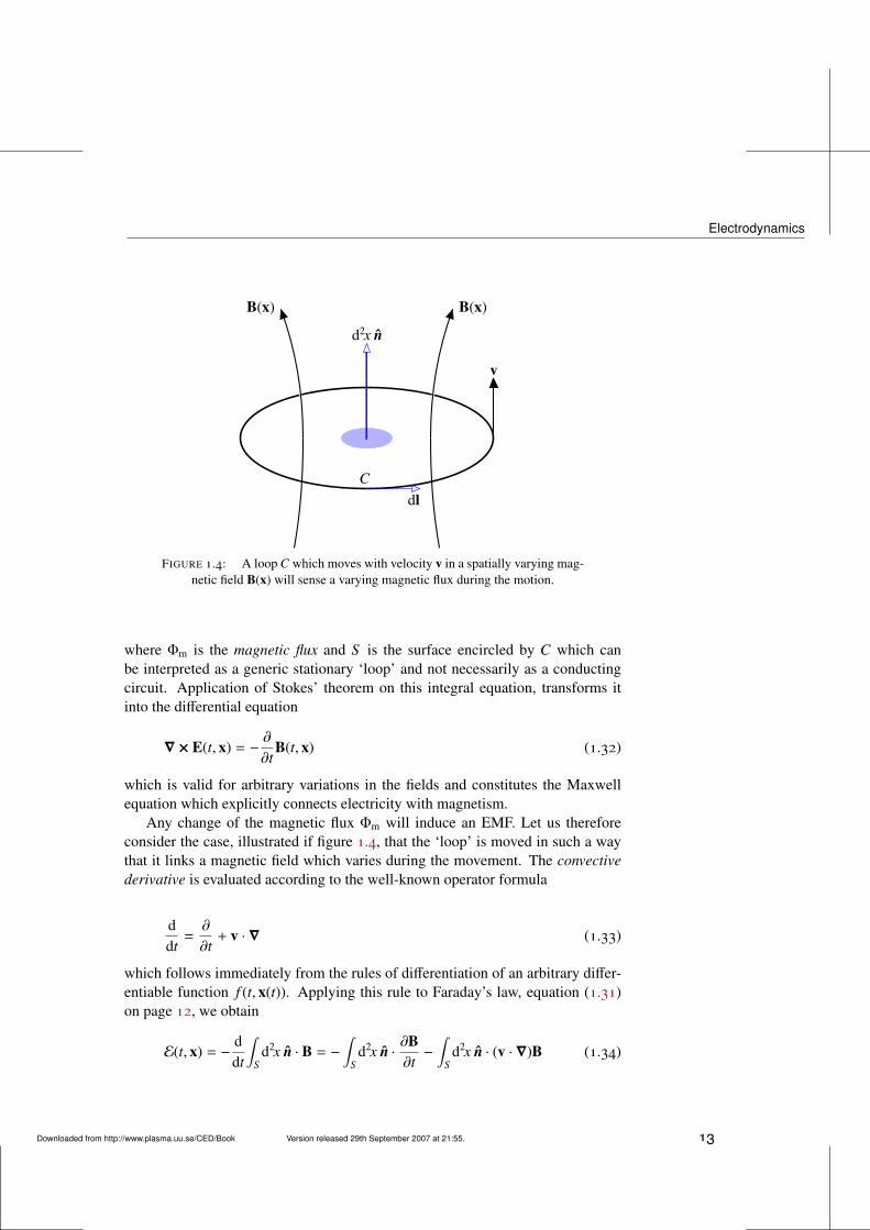
FIGURE 1.4: A loop C which moves with velocity v in a spatially varying mag-netic field B(x) will sense a varying magnetic flux during the motion.
where Φm is the magnetic flux and S is the surface encircled by C which canbe interpreted as a generic stationary ‘loop’ and not necessarily as a conductingcircuit. Application of Stokes’ theorem on this integral equation, transforms itinto the differential equation
∇ × E(t, x) = −∂
∂tB(t, x) (1.32)
which is valid for arbitrary variations in the fields and constitutes the Maxwellequation which explicitly connects electricity with magnetism.
Any change of the magnetic flux Φm will induce an EMF. Let us thereforeconsider the case, illustrated if figure 1.4, that the ‘loop’ is moved in such a waythat it links a magnetic field which varies during the movement. The convectivederivative is evaluated according to the well-known operator formula
ddt=∂
∂t+ v · ∇ (1.33)
which follows immediately from the rules of differentiation of an arbitrary differ-entiable function f (t, x(t)). Applying this rule to Faraday’s law, equation (1.31)on page 12, we obtain
E(t, x) = −ddt
∫S
d2x n · B = −∫
Sd2x n ·
∂B∂t−
∫S
d2x n · (v · ∇)B (1.34)
Downloaded from http://www.plasma.uu.se/CED/Book Version released 29th September 2007 at 21:55. 13
1. Classical Electrodynamics
During spatial differentiation v is to be considered as constant, and equa-tion (1.17) on page 8 holds also for time-varying fields:
∇ · B(t, x) = 0 (1.35)
(it is one of Maxwell’s equations) so that, according to formula (F.59) on page 181,
∇ × (B × v) = (v · ∇)B (1.36)
allowing us to rewrite equation (1.34) on page 13 in the following way:
E(t, x) =∮
Cdl · EEMF = −
ddt
∫S
d2x n · B
= −
∫S
d2x n ·∂B∂t−
∫S
d2x n · ∇ × (B × v)(1.37)
With Stokes’ theorem applied to the last integral, we finally get
E(t, x) =∮
Cdl · EEMF = −
∫S
d2x n ·∂B∂t−
∮C
dl · (B × v) (1.38)
or, rearranging the terms,∮C
dl · (EEMF − v × B) = −∫
Sd2x n ·
∂B∂t
(1.39)
where EEMF is the field which is induced in the ‘loop’, i.e., in the moving system.The use of Stokes’ theorem ‘backwards’ on equation (1.39) above yields
∇ × (EEMF − v × B) = −∂B∂t
(1.40)
In the fixed system, an observer measures the electric field
E = EEMF − v × B (1.41)
Hence, a moving observer measures the following Lorentz force on a charge q
qEEMF = qE + q(v × B) (1.42)
corresponding to an ‘effective’ electric field in the ‘loop’ (moving observer)
EEMF = E + v × B (1.43)
Hence, we can conclude that for a stationary observer, the Maxwell equation
∇ × E = −∂B∂t
(1.44)
is indeed valid even if the ‘loop’ is moving.
14 Version released 29th September 2007 at 21:55. Downloaded from http://www.plasma.uu.se/CED/Book
Electrodynamics
1.3.5 Maxwell’s microscopic equationsWe are now able to collect the results from the above considerations and formulatethe equations of classical electrodynamics valid for arbitrary variations in time andspace of the coupled electric and magnetic fields E(t, x) and B(t, x). The equationsare
∇ · E =ρ
ε0(1.45a)
∇ × E = −∂B∂t
(1.45b)
∇ · B = 0 (1.45c)
∇ × B = ε0µ0∂E∂t+ µ0j(t, x) (1.45d)
In these equations ρ(t, x) represents the total, possibly both time and space depen-dent, electric charge, i.e., free as well as induced (polarisation) charges, and j(t, x)represents the total, possibly both time and space dependent, electric current, i.e.,conduction currents (motion of free charges) as well as all atomistic (polarisation,magnetisation) currents. As they stand, the equations therefore incorporate theclassical interaction between all electric charges and currents in the system andare called Maxwell’s microscopic equations. Another name often used for themis the Maxwell-Lorentz equations. Together with the appropriate constitutive re-lations, which relate ρ and j to the fields, and the initial and boundary conditionspertinent to the physical situation at hand, they form a system of well-posed partialdifferential equations which completely determine E and B.
1.3.6 Maxwell’s macroscopic equationsThe microscopic field equations (1.45) provide a correct classical picture for arbi-trary field and source distributions, including both microscopic and macroscopicscales. However, for macroscopic substances it is sometimes convenient to intro-duce new derived fields which represent the electric and magnetic fields in which,in an average sense, the material properties of the substances are already included.These fields are the electric displacement D and the magnetising field H. In themost general case, these derived fields are complicated nonlocal, nonlinear func-tionals of the primary fields E and B:
D = D[t, x; E,B] (1.46a)
H = H[t, x; E,B] (1.46b)
Under certain conditions, for instance for very low field strengths, we may assumethat the response of a substance to the fields may be approximated as a linear one
Downloaded from http://www.plasma.uu.se/CED/Book Version released 29th September 2007 at 21:55. 15
1. Classical Electrodynamics
so that
D = εE (1.47)
H = µ−1B (1.48)
i.e., that the derived fields are linearly proportional to the primary fields and thatthe electric displacement (magnetising field) is only dependent on the electric(magnetic) field.
The field equations expressed in terms of the derived field quantities D and Hare
∇ · D = ρ(t, x) (1.49a)
∇ × E = −∂B∂t
(1.49b)
∇ · B = 0 (1.49c)
∇ ×H =∂D∂t+ j(t, x) (1.49d)
and are called Maxwell’s macroscopic equations. We will study them in moredetail in chapter 4.
1.4 Electromagnetic dualityIf we look more closely at the microscopic Maxwell equations (1.45), we see thatthey exhibit a certain, albeit not complete, symmetry. Let us follow Dirac andmake the ad hoc assumption that there exist magnetic monopoles represented bya magnetic charge density, which we denote by ρm = ρm(t, x), and a magneticcurrent density, which we denote by jm = jm(t, x). With these new quantities in-cluded in the theory, and with the electric charge density denoted ρe and the elec-tric current density denoted je, the Maxwell equations will be symmetrised intothe following two scalar and two vector, coupled, partial differential equations:
∇ · E =ρe
ε0(1.50a)
∇ × E = −∂B∂t− µ0jm (1.50b)
∇ · B = µ0ρm (1.50c)
∇ × B = ε0µ0∂E∂t+ µ0je (1.50d)
16 Version released 29th September 2007 at 21:55. Downloaded from http://www.plasma.uu.se/CED/Book
Electromagnetic duality
We shall call these equations Dirac’s symmetrised Maxwell equations or the elec-tromagnetodynamic equations.
Taking the divergence of (1.50b), we find that
∇ · (∇ × E) = −∂
∂t(∇ · B) − µ0∇ · jm ≡ 0 (1.51)
where we used the fact that, according to formula (F.63) on page 181, the diver-gence of a curl always vanishes. Using (1.50c) to rewrite this relation, we obtainthe magnetic monopole equation of continuity
∂ρm
∂t+ ∇ · jm = 0 (1.52)
which has the same form as that for the electric monopoles (electric charges) andcurrents, equation (1.23) on page 10.
We notice that the new equations (1.50) on page 16 exhibit the following sym-metry (recall that ε0µ0 = 1/c2):
E→ cB (1.53a)
cB→ −E (1.53b)
cρe → ρm (1.53c)
ρm → −cρe (1.53d)
cje → jm (1.53e)
jm → −cje (1.53f)
which is a particular case (θ = π/2) of the general duality transformation, alsoknown as the Heaviside-Larmor-Rainich transformation (indicted by the Hodgestar operator ?)
?E = E cos θ + cB sin θ (1.54a)
c?B = −E sin θ + cB cos θ (1.54b)
c?ρe = cρe cos θ + ρm sin θ (1.54c)?ρm = −cρe sin θ + ρm cos θ (1.54d)
c?je = cje cos θ + jm sin θ (1.54e)?jm = −cje sin θ + jm cos θ (1.54f)
which leaves the symmetrised Maxwell equations, and hence the physics theydescribe (often referred to as electromagnetodynamics), invariant. Since E and je
are (true or polar) vectors, B a pseudovector (axial vector), ρe a (true) scalar, thenρm and θ, which behaves as a mixing angle in a two-dimensional ‘charge space’,must be pseudoscalars and jm a pseudovector.
Downloaded from http://www.plasma.uu.se/CED/Book Version released 29th September 2007 at 21:55. 17
1. Classical Electrodynamics
The invariance of Dirac’s symmetrised Maxwell equations under the similaritytransformation means that the amount of magnetic monopole density ρm is irrele-vant for the physics as long as the ratio ρm/ρe = tan θ is kept constant. So whetherwe assume that the particles are only electrically charged or have also a magneticcharge with a given, fixed ratio between the two types of charges is a matter ofconvention, as long as we assume that this fraction is the same for all particles.Such particles are referred to as dyons [35]. By varying the mixing angle θ we canchange the fraction of magnetic monopoles at will without changing the laws ofelectrodynamics. For θ = 0 we recover the usual Maxwell electrodynamics as weknow it.5
1.5 Bibliography[1] J. AHARONI, The Special Theory of Relativity, second, revised ed., Dover Publica-
tions, Inc., New York, 1985, ISBN 0-486-64870-2.
[2] H. ALFVÉN AND N. HERLOFSON, Cosmic radiation and radio stars, Physical Review, 78(1950), p. 616.
[3] G. B. ARFKEN AND H. J. WEBER, Mathematical Methods for Physicists, fourth, interna-tional ed., Academic Press, Inc., San Diego, CA . . . , 1995, ISBN 0-12-059816-7.
[4] T. W. BARRETT AND D. M. GRIMES, Advanced Electromagnetism. Foundations, Theoryand Applications, World Scientific Publishing Co., Singapore, 1995, ISBN 981-02-2095-2.
[5] A. O. BARUT, Electrodynamics and Classical Theory of Fields and Particles, Dover Pub-lications, Inc., New York, NY, 1980, ISBN 0-486-64038-8.
[6] R. BECKER, Electromagnetic Fields and Interactions, Dover Publications, Inc.,New York, NY, 1982, ISBN 0-486-64290-9.
[7] D. BOHM, The Special Theory of Relativity, Routledge, New York, NY, 1996, ISBN 0-415-14809-X.
[8] M. BORN AND E. WOLF, Principles of Optics. Electromagnetic Theory of Propaga-tion, Interference and Diffraction of Light, sixth ed., Pergamon Press, Oxford,. . . , 1980,ISBN 0-08-026481-6.
5As Julian Schwinger (1918–1994) put it [36]:
‘. . . there are strong theoretical reasons to believe that magnetic charge exists in nature,and may have played an important role in the development of the universe. Searches formagnetic charge continue at the present time, emphasising that electromagnetism is veryfar from being a closed object’.
18 Version released 29th September 2007 at 21:55. Downloaded from http://www.plasma.uu.se/CED/Book
Bibliography
[9] W. E. BRITTIN, W. R. SMYTHE, AND W. WYSS, Poincaré gauge in electrodynamics,American Journal of Physics, 50 (1982), pp. 693–696.
[10] R. A. DEAN, Elements of Abstract Algebra, John Wiley & Sons, Inc., New York, NY . . . ,1967, ISBN 0-471-20452-8.
[11] A. A. EVETT, Permutation symbol approach to elementary vector analysis, AmericanJournal of Physics, 34 (1965), pp. 503–507.
[12] L. D. FADEEV AND A. A. SLAVNOV, Gauge Fields: Introduction to Quantum Theory,No. 50 in Frontiers in Physics: A Lecture Note and Reprint Series. Benjamin/CummingsPublishing Company, Inc., Reading, MA . . . , 1980, ISBN 0-8053-9016-2.
[13] V. L. GINZBURG, Applications of Electrodynamics in Theoretical Physics and Astro-physics, Revised third ed., Gordon and Breach Science Publishers, New York, London,Paris, Montreux, Tokyo and Melbourne, 1989, ISBN 2-88124-719-9.
[14] H. GOLDSTEIN, Classical Mechanics, second ed., Addison-Wesley Publishing Com-pany, Inc., Reading, MA . . . , 1981, ISBN 0-201-02918-9.
[15] W. T. GRANDY, Introduction to Electrodynamics and Radiation, Academic Press,New York and London, 1970, ISBN 0-12-295250-2.
[16] W. GREINER, Classical Electrodynamics, Springer-Verlag, New York, Berlin, Heidel-berg, 1996, ISBN 0-387-94799-X.
[17] M. GUIDRY, Gauge Field Theories: An Introduction with Applications, John Wiley& Sons, Inc., New York, NY . . . , 1991, ISBN 0-471-63117-5.
[18] E. HALLÉN, Electromagnetic Theory, Chapman & Hall, Ltd., London, 1962.
[19] F. HOYLE, SIR AND J. V. NARLIKAR, Lectures on Cosmology and Action at a DistanceElectrodynamics, World Scientific Publishing Co. Pte. Ltd, Singapore, New Jersey, Lon-don and Hong Kong, 1996, ISBN 9810-02-2573-3(pbk).
[20] J. D. JACKSON, Classical Electrodynamics, third ed., John Wiley & Sons, Inc.,New York, NY . . . , 1999, ISBN 0-471-30932-X.
[21] L. D. LANDAU AND E. M. LIFSHITZ, The Classical Theory of Fields, fourth revisedEnglish ed., vol. 2 of Course of Theoretical Physics, Pergamon Press, Ltd., Oxford . . . ,1975, ISBN 0-08-025072-6.
[22] L. LORENZ, Philosophical Magazine (1867), pp. 287–301.
[23] F. E. LOW, Classical Field Theory, John Wiley & Sons, Inc., New York, NY . . . , 1997,ISBN 0-471-59551-9.
[24] J. B. MARION AND M. A. HEALD, Classical Electromagnetic Radiation, second ed.,Academic Press, Inc. (London) Ltd., Orlando, . . . , 1980, ISBN 0-12-472257-1.
[25] J. C. MAXWELL, A dynamical theory of the electromagnetic field, Royal Society Trans-actions, 155 (1864).
Downloaded from http://www.plasma.uu.se/CED/Book Version released 29th September 2007 at 21:55. 19
1. Classical Electrodynamics
[26] J. C. MAXWELL, A Treatise on Electricity and Magnetism, third ed., vol. 1, Dover Publi-cations, Inc., New York, NY, 1954, ISBN 0-486-60636-8.
[27] J. C. MAXWELL, A Treatise on Electricity and Magnetism, third ed., vol. 2, Dover Publi-cations, Inc., New York, NY, 1954, ISBN 0-486-60637-8.
[28] D. B. MELROSE AND R. C. MCPHEDRAN, Electromagnetic Processes in Dispersive Me-dia, Cambridge University Press, Cambridge . . . , 1991, ISBN 0-521-41025-8.
[29] P. M. MORSE AND H. FESHBACH, Methods of Theoretical Physics, Part I. McGraw-HillBook Company, Inc., New York, NY . . . , 1953, ISBN 07-043316-8.
[30] H. MUIRHEAD, The Special Theory of Relativity, The Macmillan Press Ltd., London,Beccles and Colchester, 1973, ISBN 333-12845-1.
[31] C. MØLLER, The Theory of Relativity, second ed., Oxford University Press, Glasgow . . . ,1972.
[32] W. K. H. PANOFSKY AND M. PHILLIPS, Classical Electricity and Magnetism, second ed.,Addison-Wesley Publishing Company, Inc., Reading, MA . . . , 1962, ISBN 0-201-05702-6.
[33] F. ROHRLICH, Classical Charged Particles, Perseus Books Publishing, L.L.C., Reading,MA . . . , 1990, ISBN 0-201-48300-9.
[34] J. J. SAKURAI, Advanced Quantum Mechanics, Addison-Wesley Publishing Com-pany, Inc., Reading, MA . . . , 1967, ISBN 0-201-06710-2.
[35] J. SCHWINGER, A magnetic model of matter, Science, 165 (1969), pp. 757–761.
[36] J. SCHWINGER, L. L. DERAAD, JR., K. A. MILTON, AND W. TSAI, Classical Electrody-namics, Perseus Books, Reading, MA, 1998, ISBN 0-7382-0056-5.
[37] D. E. SOPER, Classical Field Theory, John Wiley & Sons, Inc., New York, London,Sydney and Toronto, 1976, ISBN 0-471-81368-0.
[38] B. SPAIN, Tensor Calculus, third ed., Oliver and Boyd, Ltd., Edinburgh and London,1965, ISBN 05-001331-9.
[39] J. A. STRATTON, Electromagnetic Theory, McGraw-Hill Book Company, Inc., NewYork, NY and London, 1953, ISBN 07-062150-0.
[40] W. E. THIRRING, Classical Mathematical Physics, Springer-Verlag, New York, Vienna,1997, ISBN 0-387-94843-0.
[41] J. VANDERLINDE, Classical Electromagnetic Theory, John Wiley & Sons, Inc., NewYork, Chichester, Brisbane, Toronto, and Singapore, 1993, ISBN 0-471-57269-1.
[42] J. A. WHEELER AND R. P. FEYNMAN, Interaction with the absorber as a mechanism forradiation, Reviews of Modern Physics, 17 (1945), pp. 157–.
[43] A. N. WHITEHEAD, Concept of Nature, Cambridge University Press, Cambridge . . . ,1920, ISBN 0-521-09245-0.
20 Version released 29th September 2007 at 21:55. Downloaded from http://www.plasma.uu.se/CED/Book
Examples
1.6 Examples
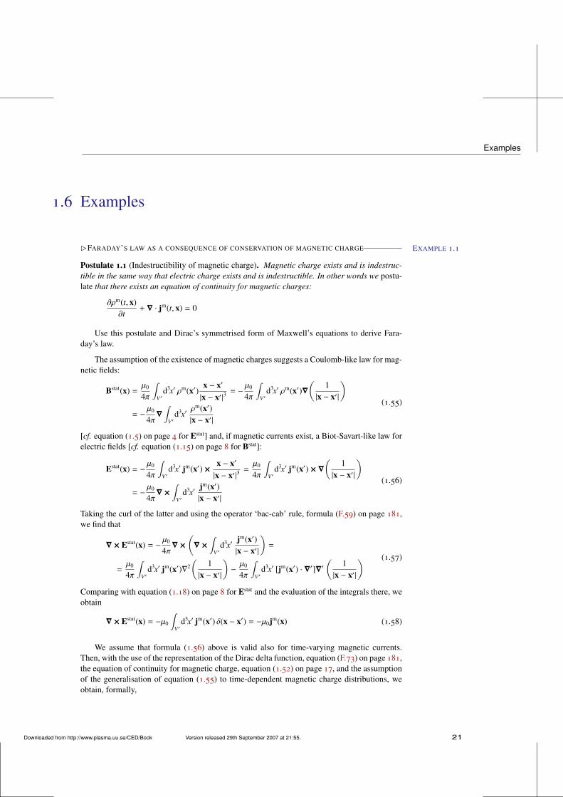
BFARADAY’S LAW AS A CONSEQUENCE OF CONSERVATION OF MAGNETIC CHARGE EXAMPLE 1.1
Postulate 1.1 (Indestructibility of magnetic charge). Magnetic charge exists and is indestruc-tible in the same way that electric charge exists and is indestructible. In other words we postu-late that there exists an equation of continuity for magnetic charges:
∂ρm(t, x)∂t
+ ∇ · jm(t, x) = 0
Use this postulate and Dirac’s symmetrised form of Maxwell’s equations to derive Fara-day’s law.
The assumption of the existence of magnetic charges suggests a Coulomb-like law for mag-netic fields:
Bstat(x) =µ0
4π
∫V′
d3x′ ρm(x′)x − x′
|x − x′|3= −
µ0
4π
∫V′
d3x′ ρm(x′)∇(
1|x − x′|
)= −
µ0
4π∇
∫V′
d3x′ρm(x′)|x − x′|
(1.55)
[cf. equation (1.5) on page 4 for Estat] and, if magnetic currents exist, a Biot-Savart-like law forelectric fields [cf. equation (1.15) on page 8 for Bstat]:
Estat(x) = −µ0
4π
∫V′
d3x′ jm(x′) ×x − x′
|x − x′|3=µ0
4π
∫V′
d3x′ jm(x′) × ∇(
1|x − x′|
)= −
µ0
4π∇ ×
∫V′
d3x′jm(x′)|x − x′|
(1.56)
Taking the curl of the latter and using the operator ‘bac-cab’ rule, formula (F.59) on page 181,we find that
∇ × Estat(x) = −µ0
4π∇ ×
(∇ ×
∫V′
d3x′jm(x′)|x − x′|
)=
=µ0
4π
∫V′
d3x′ jm(x′)∇2
(1
|x − x′|
)−µ0
4π
∫V′
d3x′ [jm(x′) · ∇′]∇′(
1|x − x′|
) (1.57)
Comparing with equation (1.18) on page 8 for Estat and the evaluation of the integrals there, weobtain
∇ × Estat(x) = −µ0
∫V′
d3x′ jm(x′) δ(x − x′) = −µ0jm(x) (1.58)
We assume that formula (1.56) above is valid also for time-varying magnetic currents.Then, with the use of the representation of the Dirac delta function, equation (F.73) on page 181,the equation of continuity for magnetic charge, equation (1.52) on page 17, and the assumptionof the generalisation of equation (1.55) to time-dependent magnetic charge distributions, weobtain, formally,
Downloaded from http://www.plasma.uu.se/CED/Book Version released 29th September 2007 at 21:55. 21
1. Classical Electrodynamics
∇ × E(t, x) = −µ0
∫V′
d3x′ jm(t, x′)δ(x − x′) −µ0
4π∂
∂t
∫V′
d3x′ ρm(t, x′)∇′(
1|x − x′|
)= −µ0jm(t, x) −
∂
∂tB(t, x)
(1.59)
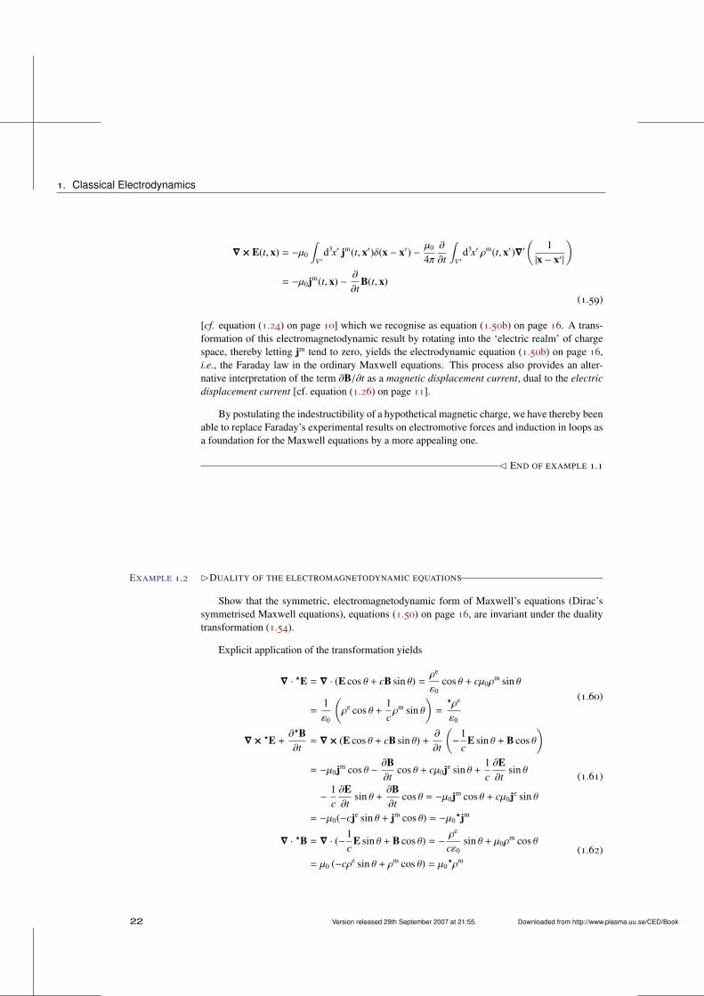
[cf. equation (1.24) on page 10] which we recognise as equation (1.50b) on page 16. A trans-formation of this electromagnetodynamic result by rotating into the ‘electric realm’ of chargespace, thereby letting jm tend to zero, yields the electrodynamic equation (1.50b) on page 16,i.e., the Faraday law in the ordinary Maxwell equations. This process also provides an alter-native interpretation of the term ∂B/∂t as a magnetic displacement current, dual to the electricdisplacement current [cf. equation (1.26) on page 11].
By postulating the indestructibility of a hypothetical magnetic charge, we have thereby beenable to replace Faraday’s experimental results on electromotive forces and induction in loops asa foundation for the Maxwell equations by a more appealing one.
C END OF EXAMPLE 1.1
BDUALITY OF THE ELECTROMAGNETODYNAMIC EQUATIONSEXAMPLE 1.2
Show that the symmetric, electromagnetodynamic form of Maxwell’s equations (Dirac’ssymmetrised Maxwell equations), equations (1.50) on page 16, are invariant under the dualitytransformation (1.54).
Explicit application of the transformation yields
∇ · ?E = ∇ · (E cos θ + cB sin θ) =ρe
ε0cos θ + cµ0ρ
m sin θ
=1ε0
(ρe cos θ +
1cρm sin θ
)=
?ρe
ε0
(1.60)
∇ ×?E +
∂?B∂t= ∇ × (E cos θ + cB sin θ) +
∂
∂t
(−
1c
E sin θ + B cos θ)
= −µ0jm cos θ −∂B∂t
cos θ + cµ0je sin θ +1c∂E∂t
sin θ
−1c∂E∂t
sin θ +∂B∂t
cos θ = −µ0jm cos θ + cµ0je sin θ
= −µ0(−cje sin θ + jm cos θ) = −µ0?jm
(1.61)
∇ · ?B = ∇ · (−1c
E sin θ + B cos θ) = −ρe
cε0sin θ + µ0ρ
m cos θ
= µ0 (−cρe sin θ + ρm cos θ) = µ0?ρm
(1.62)
22 Version released 29th September 2007 at 21:55. Downloaded from http://www.plasma.uu.se/CED/Book
Examples
∇ ×?B −
1c2
∂?E∂t= ∇ × (−
1c
E sin θ + B cos θ) −1c2
∂
∂t(E cos θ + cB sin θ)
=1cµ0jm sin θ +
1c∂B∂t
cos θ + µ0je cos θ +1c2
∂E∂t
cos θ
−1c2
∂E∂t
cos θ −1c∂B∂t
sin θ
= µ0
(1c
jm sin θ + je cos θ)= µ0
?je
(1.63)
QED
C END OF EXAMPLE 1.2
BDIRAC’S SYMMETRISED MAXWELL EQUATIONS FOR A FIXED MIXING ANGLE EXAMPLE 1.3
Show that for a fixed mixing angle θ such that
ρm = cρe tan θ (1.64a)
jm = cje tan θ (1.64b)
the symmetrised Maxwell equations reduce to the usual Maxwell equations.
Explicit application of the fixed mixing angle conditions on the duality transformation(1.54) on page 17 yields
?ρe = ρe cos θ +1cρm sin θ = ρe cos θ +
1c
cρe tan θ sin θ
=1
cos θ(ρe cos2 θ + ρe sin2 θ) =
1cos θ
ρe(1.65a)
?ρm = −cρe sin θ + cρe tan θ cos θ = −cρe sin θ + cρe sin θ = 0 (1.65b)
?je = je cos θ + je tan θ sin θ =1
cos θ(je cos2 θ + je sin2 θ) =
1cos θ
je (1.65c)
?jm = −cje sin θ + cje tan θ cos θ = −cje sin θ + cje sin θ = 0 (1.65d)
Hence, a fixed mixing angle, or, equivalently, a fixed ratio between the electric and magneticcharges/currents, ‘hides’ the magnetic monopole influence (ρm and jm) on the dynamic equa-tions.
We notice that the inverse of the transformation given by equation (1.54) on page 17 yields
E = ?E cos θ − c?B sin θ (1.66)
This means that
∇ · E = ∇ · ?E cos θ − c∇ · ?B sin θ (1.67)
Furthermore, from the expressions for the transformed charges and currents above, we find that
∇ · ?E =?ρe
ε0=
1cos θ
ρe
ε0(1.68)
Downloaded from http://www.plasma.uu.se/CED/Book Version released 29th September 2007 at 21:55. 23
1. Classical Electrodynamics
and
∇ · ?B = µ0?ρm = 0 (1.69)
so that
∇ · E =1
cos θρe
ε0cos θ − 0 =
ρe
ε0(1.70)
and so on for the other equations. QED
C END OF EXAMPLE 1.3
BCOMPLEX FIELD SIX-VECTOR FORMALISMEXAMPLE 1.4
It is sometimes convenient to introduce the complex field six-vector, also known as theRiemann-Silberstein vector
G(t, x) = E(t, x) + icB(t, x) (1.71)
where E,B ∈ R3 and hence G ∈ C3. One fundamental property of C3 is that inner (scalar)products in this space are invariant just as they are in R3. However, as discussed in example M.3on page 197, the inner (scalar) product in C3 can be defined in two different ways. Consideringthe special case of the scalar product of G with itself, we have the following two possibilitiesof defining (the square of) the ‘length’ of G:
1. The inner (scalar) product defined as G scalar multiplied with itself
G ·G = (E + icB) · (E + icB) = E2 − c2B2 + 2icE · B (1.72)
Since this is an invariant scalar quantity, we find that
E2 − c2B2 = Const (1.73a)
E · B = Const (1.73b)
2. The inner (scalar) product defined as G scalar multiplied with the complex conjugate ofitself
G ·G∗ = (E + icB) · (E − icB) = E2 + c2B2 (1.74)
which is also an invariant scalar quantity. As we shall see later, this quantity is propor-tional to the electromagnetic field energy, which indeed is a conserved quantity.
3. As with any vector, the cross product of G with itself vanishes:
G ×G = (E + icB) × (E + icB)
= E × E − c2B × B + ic(E × B) + ic(B × E)
= 0 + 0 + ic(E × B) − ic(E × B) = 0(1.75)
4. The cross product of G with the complex conjugate of itself
24 Version released 29th September 2007 at 21:55. Downloaded from http://www.plasma.uu.se/CED/Book
Examples
G ×G∗ = (E + icB) × (E − icB)
= E × E + c2B × B − ic(E × B) + ic(B × E)
= 0 + 0 − ic(E × B) − ic(E × B) = −2ic(E × B)
(1.76)
is proportional to the electromagnetic power flux, to be introduced later.
C END OF EXAMPLE 1.4
BDUALITY EXPRESSED IN THE COMPLEX FIELD SIX-VECTOR EXAMPLE 1.5
Expressed in the Riemann-Silberstein complex field vector, introduced in example 1.4 onpage 24, the duality transformation equations (1.54) on page 17 become
?G = ?E + ic?B = E cos θ + cB sin θ − iE sin θ + icB cos θ
= E(cos θ − i sin θ) + icB(cos θ − i sin θ) = e−iθ(E + icB) = e−iθG(1.77)
from which it is easy to see that
?G · ?G∗ =∣∣?G∣∣2 = e−iθG · eiθG∗ = |G|2 (1.78)
while
?G · ?G = e−2iθG ·G (1.79)
Furthermore, assuming that θ = θ(t, x), we see that the spatial and temporal differentiationof ?G leads to
∂t?G ≡
∂?G∂t= −i(∂tθ)e−iθG + e−iθ∂tG (1.80a)
∂ · ?G ≡ ∇ · ?G = −ie−iθ∇θ ·G + e−iθ
∇ ·G (1.80b)
∂ × ?G ≡ ∇ × ?G = −ie−iθ∇θ ×G + e−iθ
∇ ×G (1.80c)
which means that ∂t?G transforms as ?G itself only if θ is time-independent, and that ∇ · ?G
and ∇ × ?G transform as ?G itself only if θ is space-independent.
C END OF EXAMPLE 1.5
Downloaded from http://www.plasma.uu.se/CED/Book Version released 29th September 2007 at 21:55. 25

Downloaded from http://www.plasma.uu.se/CED/Book Version released 29th September 2007 at 21:55.
2Electromagnetic
Waves
In this chapter we investigate the dynamical properties of the electromagnetic fieldby deriving a set of equations which are alternatives to the Maxwell equations. Itturns out that these alternative equations are wave equations, indicating that elec-tromagnetic waves are natural and common manifestations of electrodynamics.
Maxwell’s microscopic equations [cf. equations (1.45) on page 15] are
∇ · E =ρ(t, x)ε0
(Gauss’s law) (2.1a)
∇ × E = −∂B∂t
(Faraday’s law) (2.1b)
∇ · B = 0 (No free magnetic charges) (2.1c)
∇ × B = µ0j(t, x) + ε0µ0∂E∂t
(Maxwell’s law) (2.1d)
and can be viewed as an axiomatic basis for classical electrodynamics. They de-scribe, in scalar and vector differential equation form, the electric and magneticfields E and B produced by given, prescribed charge distributions ρ(t, x) and cur-rent distributions j(t, x) with arbitrary time and space dependences.
However, as is well known from the theory of differential equations, these fourfirst order, coupled partial differential vector equations can be rewritten as two un-coupled, second order partial equations, one for E and one for B. We shall derivethese second order equations which, as we shall see are wave equations, and thendiscuss the implications of them. We show that for certain media, the B wave fieldcan be easily obtained from the solution of the E wave equation.
27
2. Electromagnetic Waves
2.1 The wave equationsWe restrict ourselves to derive the wave equations for the electric field vector Eand the magnetic field vector B in an electrically neutral region, i.e., a volumewhere there is no net charge, ρ = 0, and no electromotive force EEMF = 0.
2.1.1 The wave equation for EIn order to derive the wave equation for E we take the curl of (2.1b) and use (2.1d),to obtain
∇ × (∇ × E) = −∂
∂t(∇ × B) = −µ0
∂
∂t
(j + ε0
∂
∂tE)
(2.2)
According to the operator triple product ‘bac-cab’ rule equation (F.64) on page 181
∇ × (∇ × E) = ∇(∇ · E) − ∇2E (2.3)
Furthermore, since ρ = 0, equation (2.1a) on page 27 yields
∇ · E = 0 (2.4)
and since EEMF = 0, Ohm’s law, equation (1.28) on page 12, allows us to use theapproximation
j = σE (2.5)
we find that equation (2.2) above can be rewritten
∇2E − µ0∂
∂t
(σE + ε0
∂
∂tE)= 0 (2.6)
or, also using equation (1.11) on page 6 and rearranging,
∇2E − µ0σ∂E∂t−
1c2
∂2E∂t2 = 0 (2.7)
which is the homogeneous wave equation for E in a uncharged, conducting mediumwithout EMF. For waves propagating in vacuum (no charges, no currents), thewave equation for E is
∇2E −1c2
∂2E∂t2 = −
2E = 0 (2.8)
where 2 is the d’Alembert operator, defined according to formula (M.93) onpage 199.
28 Version released 29th September 2007 at 21:55. Downloaded from http://www.plasma.uu.se/CED/Book
The wave equations
2.1.2 The wave equation for BThe wave equation for B is derived in much the same way as the wave equationfor E. Take the curl of (2.1d) and use Ohm’s law j = σE to obtain
∇ × (∇ × B) = µ0∇ × j + ε0µ0∂
∂t(∇ × E) = µ0σ∇ × E + ε0µ0
∂
∂t(∇ × E)
(2.9)
which, with the use of equation (F.64) on page 181 and equation (2.1c) on page 27can be rewritten
∇(∇ · B) − ∇2B = −µ0σ∂B∂t− ε0µ0
∂2
∂t2 B (2.10)
Using the fact that, according to (2.1c), ∇ ·B = 0 for any medium and rearranging,we can rewrite this equation as
∇2B − µ0σ∂B∂t−
1c2
∂2B∂t2 = 0 (2.11)
This is the wave equation for the magnetic field. For waves propagating in vacuum(no charges, no currents), the wave equation for B is
∇2B −1c2
∂2B∂t2 = −
2B = 0 (2.12)
We notice that for the simple propagation media considered here, the waveequations for the magnetic field B has exactly the same mathematical form as thewave equation for the electric field E, equation (2.7) on page 28. Therefore, it suf-fices to consider only the E field, since the results for the B field follow trivially.For EM waves propagating in more complicated media, containing, eg., inhomo-geneities, the wave equation for E and for B do not have the same mathematicalform.
2.1.3 The time-independent wave equation for EIf we assume that the temporal dependence of E (and B) is well-behaved enoughthat it can be represented by a sum of a finite number of temporal spectral (Fourier)components, i.e., in the form of a temporal Fourier series, then it is sufficient torepresent the electric field by one of these Fourier components
E(t, x) = E0(x) cos(ωt) = E0(x)Re
e−iωt (2.13)
since the general solution is obtained by a linear superposition (summation) of theresult for one such spectral (Fourier) component, often called a time-harmonic
Downloaded from http://www.plasma.uu.se/CED/Book Version released 29th September 2007 at 21:55. 29
2. Electromagnetic Waves
wave. When we insert this, in complex notation, into equation (2.7) on page 28we find that
∇2E0(x)e−iωt − µ0σ∂
∂tE0(x)e−iωt −
1c2
∂2
∂t2 E0(x)e−iωt
= ∇2E0(x)e−iωt − µ0σ(−iω)E0(x)e−iωt −1c2 (−iω)2E0(x)e−iωt
(2.14)
or, dividing out the common factor e−iωt and rewriting,
∇2E0 +ω2
c2
(1 + i
σ
ε0ω
)E0 = 0 (2.15)
Multiplying by e−iωt and introducing the relaxation time τ = ε0/σ of the mediumin question, we see that the differential equation for the time-harmonic wave canbe written
∇2E(t, x) +ω2
c2
(1 +
iτω
)E(t, x) = 0 (2.16)
In the limit of very many frequency components the Fourier sum goes overinto a Fourier integral. To illustrate this general case, let us introduce the Fouriertransform of E(t, x)
F [E(t, x)]def≡ Ew(x) =
12π
∫ ∞−∞
dt E(t, x) eiωt (2.17)
and the corresponding inverse Fourier transform
F −1[Eω(x)]def≡ E(t, x) =
∫ ∞−∞
dωEω(x) e−iωt (2.18)
Then we find that the Fourier transform of ∂E(t, x)/∂t becomes
F
[∂E(t, x)∂t
]def≡
12π
∫ ∞−∞
dt(∂E(t, x)∂t
)eiωt
=1
2π[E(t, x) eiωt]∞
−∞︸ ︷︷ ︸=0
−iω1
2π
∫ ∞−∞
dt E(t, x) eiωt
= − iωEω(x)
(2.19)
and that, consequently,
F
[∂2E(t, x)∂t2
]def≡
12π
∫ ∞−∞
dt(∂2E(t, x)∂t2
)eiωt = −ω2Eω(x) (2.20)
30 Version released 29th September 2007 at 21:55. Downloaded from http://www.plasma.uu.se/CED/Book
The wave equations
Fourier transforming equation (2.7) on page 28 and using (2.19) and (2.20), weobtain
∇2Eω +ω2
c2
(1 +
iτω
)Eω = 0 (2.21)
A subsequent inverse Fourier transformation of the solution Eω of this equationleads to the same result as is obtained from the solution of equation (2.16) onpage 30. I.e., by considering just one Fourier component we obtain the resultswhich are identical to those that we would have obtained by employing the heavymachinery of Fourier transforms and Fourier integrals. Hence, under the assump-tion of linearity (superposition principle) there is no need for the heavy, time-consuming forward and inverse Fourier transform machinery.
In the limit of long τ, (2.16) tends to
∇2E +ω2
c2 E = 0 (2.22)
which is a time-independent wave equation for E, representing undamped propa-gating waves. In the short τ limit we have instead
∇2E + iωµ0σE = 0 (2.23)
which is a time-independent diffusion equation for E.For most metals τ ∼ 10−14 s, which means that the diffusion picture is good for
all frequencies lower than optical frequencies. Hence, in metallic conductors, thepropagation term ∂2E/c2∂t2 is negligible even for VHF, UHF, and SHF signals.Alternatively, we may say that the displacement current ε0∂E/∂t is negligible rel-ative to the conduction current j = σE.
If we introduce the vacuum wave number
k =ω
c(2.24)
we can write, using the fact that c = 1/√ε0µ0 according to equation (1.11) on
page 6,
1τω=
σ
ε0ω=σ
ε0
1ck=σ
k
õ0
ε0=σ
kR0 (2.25)
where in the last step we introduced the characteristic impedance for vacuum
R0 =
õ0
ε0≈ 376.7Ω (2.26)
Downloaded from http://www.plasma.uu.se/CED/Book Version released 29th September 2007 at 21:55. 31
2. Electromagnetic Waves
2.2 Plane wavesConsider now the case where all fields depend only on the distance ζ to a givenplane with unit normal n. Then the del operator becomes
∇ = n∂
∂ζ= n∇ (2.27)
and Maxwell’s equations attain the form
n ·∂E∂ζ= 0 (2.28a)
n×∂E∂ζ= −
∂B∂t
(2.28b)
n ·∂B∂ζ= 0 (2.28c)
n×∂B∂ζ= µ0j(t, x) + ε0µ0
∂E∂t= µ0σE + ε0µ0
∂E∂t
(2.28d)
Scalar multiplying (2.28d) by n, we find that
0 = n ·(
n×∂B∂ζ
)= n ·
(µ0σ + ε0µ0
∂
∂t
)E (2.29)
which simplifies to the first-order ordinary differential equation for the normalcomponent En of the electric field
dEn
dt+σ
ε0En = 0 (2.30)
with the solution
En = En0 e−σt/ε0 = En0 e−t/τ (2.31)
This, together with (2.28a), shows that the longitudinal component of E, i.e., thecomponent which is perpendicular to the plane surface is independent of ζ and hasa time dependence which exhibits an exponential decay, with a decrement givenby the relaxation time τ in the medium.
Scalar multiplying (2.28b) by n, we similarly find that
0 = n ·(
n×∂E∂ζ
)= −n ·
∂B∂t
(2.32)
or
n ·∂B∂t= 0 (2.33)
From this, and (2.28c), we conclude that the only longitudinal component of Bmust be constant in both time and space. In other words, the only non-staticsolution must consist of transverse components.
32 Version released 29th September 2007 at 21:55. Downloaded from http://www.plasma.uu.se/CED/Book
Plane waves
2.2.1 Telegrapher’s equationIn analogy with equation (2.7) on page 28, we can easily derive the equation
∂2E∂ζ2 − µ0σ
∂E∂t−
1c2
∂2E∂t2 = 0 (2.34)
This equation, which describes the propagation of plane waves in a conductingmedium, is called the telegrapher’s equation. If the medium is an insulator so thatσ = 0, then the equation takes the form of the one-dimensional wave equation
∂2E∂ζ2 −
1c2
∂2E∂t2 = 0 (2.35)
As is well known, each component of this equation has a solution which can bewritten
Ei = f (ζ − ct) + g(ζ + ct), i = 1, 2, 3 (2.36)
where f and g are arbitrary (non-pathological) functions of their respective argu-ments. This general solution represents perturbations which propagate along ζ,where the f perturbation propagates in the positive ζ direction and the g perturba-tion propagates in the negative ζ direction.
If we assume that our electromagnetic fields E and B are time-harmonic,i.e., that they can each be represented by a Fourier component proportional toexp−iωt, the solution of equation (2.35) above becomes
E = E0e−i(ωt±kζ) = E0ei(∓kζ−ωt) (2.37)
By introducing the wave vector
k = kn =ω
cn =
ω
ck (2.38)
this solution can be written as
E = E0ei(k·x−ωt) (2.39)
Let us consider the lower sign in front of kζ in the exponent in (2.37). Thiscorresponds to a wave which propagates in the direction of increasing ζ. Insertingthis solution into equation (2.28b) on page 32, gives
n×∂E∂ζ= iωB = ikn× E (2.40)
or, solving for B,
B =kω
n× E =1ω
k × E =1c
k × E =√ε0µ0 n× E (2.41)
Hence, to each transverse component of E, there exists an associated magneticfield given by equation (2.41) above. If E and/or B has a direction in space whichis constant in time, we have a plane wave.
Downloaded from http://www.plasma.uu.se/CED/Book Version released 29th September 2007 at 21:55. 33
2. Electromagnetic Waves
2.2.2 Waves in conductive mediaAssuming that our medium has a finite conductivity σ, and making the time-harmonic wave Ansatz in equation (2.34) on page 33, we find that the time-independent telegrapher’s equation can be written
∂2E∂ζ2 + ε0µ0ω
2E + iµ0σωE =∂2E∂ζ2 + K2E = 0 (2.42)
where
K2 = ε0µ0ω2(
1 + iσ
ε0ω
)=ω2
c2
(1 + i
σ
ε0ω
)= k2
(1 + i
σ
ε0ω
)(2.43)
where, in the last step, equation (2.24) on page 31 was used to introduce the wavenumber k. Taking the square root of this expression, we obtain
K = k√
1 + iσ
ε0ω= α + iβ (2.44)
Squaring, one finds that
k2(
1 + iσ
ε0ω
)= (α2 − β2) + 2iαβ (2.45)
or
β2 = α2 − k2 (2.46)
αβ =k2σ
2ε0ω(2.47)
Squaring the latter and combining with the former, one obtains the second orderalgebraic equation (in α2)
α2(α2 − k2) =k4σ2
4ε20ω
2 (2.48)
which can be easily solved and one finds that
α = k
√√√√√√
1 +(
σε0ω
)2+ 1
2(2.49a)
β = k
√√√√√√
1 +(
σε0ω
)2− 1
2(2.49b)
34 Version released 29th September 2007 at 21:55. Downloaded from http://www.plasma.uu.se/CED/Book
Observables and averages
As a consequence, the solution of the time-independent telegrapher’s equation,equation (2.42) on page 34, can be written
E = E0e−βζei(αζ−ωt) (2.50)
With the aid of equation (2.41) on page 33 we can calculate the associated mag-netic field, and find that it is given by
B =1ω
K k × E =1ω
(k × E)(α + iβ) =1ω
(k × E) |A| eiγ (2.51)
where we have, in the last step, rewritten α + iβ in the amplitude-phase form|A| expiγ. From the above, we immediately see that E, and consequently also B,is damped, and that E and B in the wave are out of phase.
In the limit ε0ω σ, we can approximate K as follows:
K = k(
1 + iσ
ε0ω
) 12
= k[
iσ
ε0ω
(1 − i
ε0ω
σ
)] 12
≈ k(1 + i)√
σ
2ε0ω
=√ε0µ0ω(1 + i)
√σ
2ε0ω= (1 + i)
√µ0σω
2
(2.52)
In this limit we find that when the wave impinges perpendicularly upon the medium,the fields are given, inside the medium, by
E′ = E0 exp−
√µ0σω
2ζ
exp
i(√
µ0σω
2ζ − ωt
)(2.53a)
B′ = (1 + i)√µ0σ
2ω(n× E′) (2.53b)
Hence, both fields fall off by a factor 1/e at a distance
δ =
√2
µ0σω(2.54)
This distance δ is called the skin depth.
2.3 Observables and averagesIn the above we have used complex notation quite extensively. This is for mathe-matical convenience only. For instance, in this notation differentiations are almosttrivial to perform. However, every physical measurable quantity is always real
Downloaded from http://www.plasma.uu.se/CED/Book Version released 29th September 2007 at 21:55. 35
2. Electromagnetic Waves
valued. I.e., ‘Ephysical = Re Emathematical’. It is particularly important to remem-ber this when one works with products of physical quantities. For instance, ifwe have two physical vectors F and G which both are time-harmonic, i.e., can berepresented by Fourier components proportional to exp−iωt, then we must makethe following interpretation
F(t, x) ·G(t, x) = Re F · Re G = Re
F0(x) e−iωt · Re
G0(x) e−iωt(2.55)
Furthermore, letting ∗ denote complex conjugate, we can express the real part ofthe complex vector F as
Re F = Re
F0(x) e−iωt = 12
[F0(x) e−iωt + F∗0(x) eiωt] (2.56)
and similarly for G. Hence, the physically acceptable interpretation of the scalarproduct of two complex vectors, representing physical observables, is
F(t, x) ·G(t, x) = Re
F0(x) e−iωt · Re
G0(x) e−iωt=
12
[F0(x) e−iωt + F∗0(x) eiωt] ·12
[G0(x) e−iωt +G∗0(x) eiωt]
=14(F0 ·G∗0 + F∗0 ·G0 + F0 ·G0 e−2iωt + F∗0 ·G
∗0 e2iωt)
=12
Re
F0 ·G∗0 + F0 ·G0 e−2iωt=
12
Re
F0 e−iωt ·G∗0 eiωt + F0 ·G0 e−2iωt=
12
Re
F(t, x) ·G∗(t, x) + F0 ·G0 e−2iωt(2.57)
Often in physics, we measure temporal averages (〈 〉) of our physical observ-ables. If so, we see that the average of the product of the two physical quantitiesrepresented by F and G can be expressed as
〈F ·G〉 ≡ 〈Re F · Re G〉 =12
Re F ·G∗ =12
F ·G∗ =12
F∗ ·G (2.58)
since the temporal average of the oscillating function exp−2iωt vanishes.
2.4 Bibliography[1] J. AHARONI, The Special Theory of Relativity, second, revised ed., Dover Publica-
tions, Inc., New York, 1985, ISBN 0-486-64870-2.
36 Version released 29th September 2007 at 21:55. Downloaded from http://www.plasma.uu.se/CED/Book
Bibliography
[2] H. ALFVÉN AND N. HERLOFSON, Cosmic radiation and radio stars, Physical Review, 78(1950), p. 616.
[3] G. B. ARFKEN AND H. J. WEBER, Mathematical Methods for Physicists, fourth, interna-tional ed., Academic Press, Inc., San Diego, CA . . . , 1995, ISBN 0-12-059816-7.
[4] T. W. BARRETT AND D. M. GRIMES, Advanced Electromagnetism. Foundations, Theoryand Applications, World Scientific Publishing Co., Singapore, 1995, ISBN 981-02-2095-2.
[5] A. O. BARUT, Electrodynamics and Classical Theory of Fields and Particles, Dover Pub-lications, Inc., New York, NY, 1980, ISBN 0-486-64038-8.
[6] R. BECKER, Electromagnetic Fields and Interactions, Dover Publications, Inc.,New York, NY, 1982, ISBN 0-486-64290-9.
[7] D. BOHM, The Special Theory of Relativity, Routledge, New York, NY, 1996, ISBN 0-415-14809-X.
[8] M. BORN AND E. WOLF, Principles of Optics. Electromagnetic Theory of Propaga-tion, Interference and Diffraction of Light, sixth ed., Pergamon Press, Oxford,. . . , 1980,ISBN 0-08-026481-6.
[9] W. E. BRITTIN, W. R. SMYTHE, AND W. WYSS, Poincaré gauge in electrodynamics,American Journal of Physics, 50 (1982), pp. 693–696.
[10] R. A. DEAN, Elements of Abstract Algebra, John Wiley & Sons, Inc., New York, NY . . . ,1967, ISBN 0-471-20452-8.
[11] A. A. EVETT, Permutation symbol approach to elementary vector analysis, AmericanJournal of Physics, 34 (1965), pp. 503–507.
[12] L. D. FADEEV AND A. A. SLAVNOV, Gauge Fields: Introduction to Quantum Theory,No. 50 in Frontiers in Physics: A Lecture Note and Reprint Series. Benjamin/CummingsPublishing Company, Inc., Reading, MA . . . , 1980, ISBN 0-8053-9016-2.
[13] V. L. GINZBURG, Applications of Electrodynamics in Theoretical Physics and Astro-physics, Revised third ed., Gordon and Breach Science Publishers, New York, London,Paris, Montreux, Tokyo and Melbourne, 1989, ISBN 2-88124-719-9.
[14] H. GOLDSTEIN, Classical Mechanics, second ed., Addison-Wesley Publishing Com-pany, Inc., Reading, MA . . . , 1981, ISBN 0-201-02918-9.
[15] W. T. GRANDY, Introduction to Electrodynamics and Radiation, Academic Press,New York and London, 1970, ISBN 0-12-295250-2.
[16] W. GREINER, Classical Electrodynamics, Springer-Verlag, New York, Berlin, Heidel-berg, 1996, ISBN 0-387-94799-X.
[17] M. GUIDRY, Gauge Field Theories: An Introduction with Applications, John Wiley& Sons, Inc., New York, NY . . . , 1991, ISBN 0-471-63117-5.
Downloaded from http://www.plasma.uu.se/CED/Book Version released 29th September 2007 at 21:55. 37
2. Electromagnetic Waves
[18] E. HALLÉN, Electromagnetic Theory, Chapman & Hall, Ltd., London, 1962.
[19] F. HOYLE, SIR AND J. V. NARLIKAR, Lectures on Cosmology and Action at a DistanceElectrodynamics, World Scientific Publishing Co. Pte. Ltd, Singapore, New Jersey, Lon-don and Hong Kong, 1996, ISBN 9810-02-2573-3(pbk).
[20] J. D. JACKSON, Classical Electrodynamics, third ed., John Wiley & Sons, Inc.,New York, NY . . . , 1999, ISBN 0-471-30932-X.
[21] L. D. LANDAU AND E. M. LIFSHITZ, The Classical Theory of Fields, fourth revisedEnglish ed., vol. 2 of Course of Theoretical Physics, Pergamon Press, Ltd., Oxford . . . ,1975, ISBN 0-08-025072-6.
[22] L. LORENZ, Philosophical Magazine (1867), pp. 287–301.
[23] F. E. LOW, Classical Field Theory, John Wiley & Sons, Inc., New York, NY . . . , 1997,ISBN 0-471-59551-9.
[24] J. B. MARION AND M. A. HEALD, Classical Electromagnetic Radiation, second ed.,Academic Press, Inc. (London) Ltd., Orlando, . . . , 1980, ISBN 0-12-472257-1.
[25] J. C. MAXWELL, A dynamical theory of the electromagnetic field, Royal Society Trans-actions, 155 (1864).
[26] J. C. MAXWELL, A Treatise on Electricity and Magnetism, third ed., vol. 1, Dover Publi-cations, Inc., New York, NY, 1954, ISBN 0-486-60636-8.
[27] J. C. MAXWELL, A Treatise on Electricity and Magnetism, third ed., vol. 2, Dover Publi-cations, Inc., New York, NY, 1954, ISBN 0-486-60637-8.
[28] D. B. MELROSE AND R. C. MCPHEDRAN, Electromagnetic Processes in Dispersive Me-dia, Cambridge University Press, Cambridge . . . , 1991, ISBN 0-521-41025-8.
[29] P. M. MORSE AND H. FESHBACH, Methods of Theoretical Physics, Part I. McGraw-HillBook Company, Inc., New York, NY . . . , 1953, ISBN 07-043316-8.
[30] H. MUIRHEAD, The Special Theory of Relativity, The Macmillan Press Ltd., London,Beccles and Colchester, 1973, ISBN 333-12845-1.
[31] C. MØLLER, The Theory of Relativity, second ed., Oxford University Press, Glasgow . . . ,1972.
[32] W. K. H. PANOFSKY AND M. PHILLIPS, Classical Electricity and Magnetism, second ed.,Addison-Wesley Publishing Company, Inc., Reading, MA . . . , 1962, ISBN 0-201-05702-6.
[33] F. ROHRLICH, Classical Charged Particles, Perseus Books Publishing, L.L.C., Reading,MA . . . , 1990, ISBN 0-201-48300-9.
[34] J. J. SAKURAI, Advanced Quantum Mechanics, Addison-Wesley Publishing Com-pany, Inc., Reading, MA . . . , 1967, ISBN 0-201-06710-2.
[35] J. SCHWINGER, A magnetic model of matter, Science, 165 (1969), pp. 757–761.
38 Version released 29th September 2007 at 21:55. Downloaded from http://www.plasma.uu.se/CED/Book
Bibliography
[36] J. SCHWINGER, L. L. DERAAD, JR., K. A. MILTON, AND W. TSAI, Classical Electrody-namics, Perseus Books, Reading, MA, 1998, ISBN 0-7382-0056-5.
[37] D. E. SOPER, Classical Field Theory, John Wiley & Sons, Inc., New York, London,Sydney and Toronto, 1976, ISBN 0-471-81368-0.
[38] B. SPAIN, Tensor Calculus, third ed., Oliver and Boyd, Ltd., Edinburgh and London,1965, ISBN 05-001331-9.
[39] J. A. STRATTON, Electromagnetic Theory, McGraw-Hill Book Company, Inc., NewYork, NY and London, 1953, ISBN 07-062150-0.
[40] W. E. THIRRING, Classical Mathematical Physics, Springer-Verlag, New York, Vienna,1997, ISBN 0-387-94843-0.
[41] J. VANDERLINDE, Classical Electromagnetic Theory, John Wiley & Sons, Inc., NewYork, Chichester, Brisbane, Toronto, and Singapore, 1993, ISBN 0-471-57269-1.
[42] J. A. WHEELER AND R. P. FEYNMAN, Interaction with the absorber as a mechanism forradiation, Reviews of Modern Physics, 17 (1945), pp. 157–.
[43] A. N. WHITEHEAD, Concept of Nature, Cambridge University Press, Cambridge . . . ,1920, ISBN 0-521-09245-0.
Downloaded from http://www.plasma.uu.se/CED/Book Version released 29th September 2007 at 21:55. 39
2. Electromagnetic Waves
2.5 Example
BWAVE EQUATIONS IN ELECTROMAGNETODYNAMICSEXAMPLE 2.1
Derive the wave equation for the E field described by the electromagnetodynamic equations(Dirac’s symmetrised Maxwell equations) [cf. equations (1.50) on page 16]
∇ · E =ρe
ε0(2.59a)
∇ × E = −∂B∂t− µ0jm (2.59b)
∇ · B = µ0ρm (2.59c)
∇ × B = ε0µ0∂E∂t+ µ0je (2.59d)
under the assumption of vanishing net electric and magnetic charge densities and in the absenceof electromotive and magnetomotive forces. Interpret this equation physically.
Taking the curl of (2.59b) and using (2.59d), and assuming, for symmetry reasons, thatthere exists a linear relation between the magnetic current density jm and the magnetic field B(the magnetic dual of Ohm’s law for electric currents, je = σeE)
jm = σmB (2.60)
one finds, noting that ε0µ0 = 1/c2, that
∇ × (∇ × E) = −µ0∇ × jm −∂
∂t(∇ × B) = −µ0σ
m∇ × B −
∂
∂t
(µ0je +
1c2
∂E∂t
)= −µ0σ
m
(µ0σ
eE +1c2
∂E∂t
)− µ0σ
e ∂E∂t−
1c2
∂2E∂t2
(2.61)
Using the vector operator identity ∇ × (∇ × E) = ∇(∇ · E) − ∇2E, and the fact that ∇ · E = 0for a vanishing net electric charge, we can rewrite the wave equation as
∇2E − µ0
(σe +
σm
c2
)∂E∂t−
1c2
∂2E∂t2 − µ
20σ
mσeE = 0 (2.62)
This is the homogeneous electromagnetodynamic wave equation for E we were after.
Compared to the ordinary electrodynamic wave equation for E, equation (2.7) on page 28,we see that we pick up extra terms. In order to understand what these extra terms mean phys-ically, we analyse the time-independent wave equation for a single Fourier component. Thenour wave equation becomes
∇2E + iωµ0
(σe +
σm
c2
)E +
ω2
c2 E − µ20σ
mσeE
= ∇2E +ω2
c2
[(1 −
1ω2
µ0
ε0σmσe
)+ i
σe + σm/c2
ε0ω
]E = 0
(2.63)
Realising that, according to formula (2.26) on page 31, µ0/ε0 is the square of the vacuumradiation resistance R0, and rearranging a bit, we obtain the time-independent wave equation in
40 Version released 29th September 2007 at 21:55. Downloaded from http://www.plasma.uu.se/CED/Book
Example
Dirac’s symmetrised electrodynamics
∇2E +ω2
c2
(1 −
R20
ω2σmσe
)1 + iσe + σm/c2
ε0ω(
1 − R20
ω2σmσe)E = 0 (2.64)
From this equation we conclude that the existence of magnetic charges (magnetic monopoles),and non-vanishing electric and magnetic conductivities would lead to a shift in the effectivewave number of the wave. Furthermore, even if the electric conductivity σe vanishes, theimaginary term does not necessarily vanish and the wave might therefore experience damping(or growth) according as σm is positive (or negative). This would happen in a hypotheticalmedium which is a perfect insulator for electric currents but which can carry magnetic currents.
Finally, we note that in the particular case that ω = R0√σmσe, the wave equation becomes
a (time-independent) diffusion equation
∇2E + iωµ0
(σe +
σm
c2
)E = 0 (2.65)
and, hence, no waves exist at all!
C END OF EXAMPLE 2.1
Downloaded from http://www.plasma.uu.se/CED/Book Version released 29th September 2007 at 21:55. 41

Downloaded from http://www.plasma.uu.se/CED/Book Version released 29th September 2007 at 21:55.
3Electromagnetic
Potentials
As an alternative to expressing the laws of electrodynamics in terms of electric andmagnetic fields, it turns out that it is often more convenient to express the theoryin terms of potentials. This is particularly true for problems related to radiation. Inthis chapter we will introduce and study the properties of such potentials and shallfind that they exhibit some remarkable properties which elucidate the fundamentalaspects of electromagnetism and lead naturally to the special theory of relativity.
3.1 The electrostatic scalar potentialAs we saw in equation (1.8) on page 6, the electrostatic field Estat(x) is irrotational.Hence, it may be expressed in terms of the gradient of a scalar field. If we denotethis scalar field by −φstat(x), we get
Estat(x) = −∇φstat(x) (3.1)
Taking the divergence of this and using equation (1.7) on page 5, we obtain Pois-son’s equation
∇2φstat(x) = −∇ · Estat(x) = −ρ(x)ε0
(3.2)
A comparison with the definition of Estat, namely equation (1.5) on page 4, showsthat this equation has the solution
φstat(x) =1
4πε0
∫V ′
d3x′ρ(x′)|x − x′|
+ α (3.3)
43
3. Electromagnetic Potentials
where the integration is taken over all source points x′ at which the charge densityρ(x′) is non-zero and α is an arbitrary quantity which has a vanishing gradient.An example of such a quantity is a scalar constant. The scalar function φstat(x) inequation (3.3) on page 43 is called the electrostatic scalar potential.
3.2 The magnetostatic vector potentialConsider the equations of magnetostatics (1.22) on page 9. From equation (F.63)on page 181 we know that any 3D vector a has the property that ∇ · (∇ × a) ≡ 0and in the derivation of equation (1.17) on page 8 in magnetostatics we found that∇ · Bstat(x) = 0. We therefore realise that we can always write
Bstat(x) = ∇ × Astat(x) (3.4)
where Astat(x) is called the magnetostatic vector potential.We saw above that the electrostatic potential (as any scalar potential) is not
unique: we may, without changing the physics, add to it a quantity whose spatialgradient vanishes. A similar arbitrariness is true also for the magnetostatic vectorpotential.
In the magnetostatic case, we may start from Biot-Savart’s law as expressed byequation (1.15) on page 8. Identifying this expression with equation (3.4) allowsus to define the static vector potential as
Astat(x) =µ0
4π
∫V ′
d3x′j(x′)|x − x′|
+ a(x) (3.5)
where a(x) is an arbitrary vector field whose curl vanishes. From equation (F.62)on page 181 we know that such a vector can always be written as the gradient ofa scalar field.
3.3 The electrodynamic potentialsLet us now generalise the static analysis above to the electrodynamic case, i.e.,the case with temporal and spatial dependent sources ρ(t, x) and j(t, x), and cor-responding fields E(t, x) and B(t, x), as described by Maxwell’s equations (1.45)on page 15. In other words, let us study the electrodynamic potentials φ(t, x) andA(t, x).
44 Version released 29th September 2007 at 21:55. Downloaded from http://www.plasma.uu.se/CED/Book
Gauge transformations
From equation (1.45c) on page 15 we note that also in electrodynamics thehomogeneous equation ∇ · B(t, x) = 0 remains valid. Because of this divergence-free nature of the time- and space-dependent magnetic field, we can express it asthe curl of an electromagnetic vector potential:
B(t, x) = ∇ × A(t, x) (3.6)
Inserting this expression into the other homogeneous Maxwell equation (1.32) onpage 13, we obtain
∇ × E(t, x) = −∂
∂t[∇ × A(t, x)] = −∇ ×
∂
∂tA(t, x) (3.7)
or, rearranging the terms,
∇ ×
(E(t, x) +
∂
∂tA(t, x)
)= 0 (3.8)
As before we utilise the vanishing curl of a vector expression to write thisvector expression as the gradient of a scalar function. If, in analogy with the elec-trostatic case, we introduce the electromagnetic scalar potential function −φ(t, x),equation (3.8) becomes equivalent to
E(t, x) +∂
∂tA(t, x) = −∇φ(t, x) (3.9)
This means that in electrodynamics, E(t, x) is calculated from the potentials ac-cording to the formula
E(t, x) = −∇φ(t, x) −∂
∂tA(t, x) (3.10)
and B(t, x) from formula (3.6) above. Hence, it is a matter of taste whether wewant to express the laws of electrodynamics in terms of the potentials φ(t, x) andA(t, x), or in terms of the fields E(t, x) and B(t, x). However, there exists an im-portant difference between the two approaches: in classical electrodynamics theonly directly observable quantities are the fields themselves (and quantities de-rived from them) and not the potentials. On the other hand, the treatment becomessignificantly simpler if we use the potentials in our calculations and then, at thefinal stage, use equation (3.6) and equation (3.10) above to calculate the fields orphysical quantities expressed in the fields.
3.4 Gauge transformationsWe saw in section 3.1 on page 43 and in section 3.2 on page 44 that in electrostat-ics and magnetostatics we have a certain mathematical degree of freedom, up to
Downloaded from http://www.plasma.uu.se/CED/Book Version released 29th September 2007 at 21:55. 45
3. Electromagnetic Potentials
terms of vanishing gradients and curls, to pick suitable forms for the potentials andstill get the same physical result. In fact, the way the electromagnetic scalar poten-tial φ(t, x) and the vector potential A(t, x) are related to the physically observablesgives leeway for similar ‘manipulation’ of them also in electrodynamics.
If we transform φ(t, x) and A(t, x) simultaneously into new ones φ′(t, x) andA′(t, x) according to the mapping scheme
φ(t, x) 7→ φ′(t, x) = φ(t, x) +∂Γ(t, x)∂t
(3.11a)
A(t, x) 7→ A′(t, x) = A(t, x) − ∇Γ(t, x) (3.11b)
where Γ(t, x) is an arbitrary, differentiable scalar function called the gauge func-tion, and insert the transformed potentials into equation (3.10) on page 45 for theelectric field and into equation (3.6) on page 45 for the magnetic field, we obtainthe transformed fields
E′ = −∇φ′ −∂A′
∂t= −∇φ −
∂(∇Γ)∂t−∂A∂t+∂(∇Γ)∂t
= −∇φ −∂A∂t
(3.12a)
B′ = ∇ × A′ = ∇ × A − ∇ × (∇Γ) = ∇ × A (3.12b)
where, once again equation (F.62) on page 181 was used. We see that the fieldsare unaffected by the gauge transformation (3.11). A transformation of the poten-tials φ and A which leaves the fields, and hence Maxwell’s equations, invariantis called a gauge transformation. A physical law which does not change under agauge transformation is said to be gauge invariant. It is only those quantities (ex-pressions) that are gauge invariant that have experimental significance. Of course,the EM fields themselves are gauge invariant.
3.5 Gauge conditionsInserting (3.10) and (3.6) on page 45 into Maxwell’s equations (1.45) on page 15we obtain, after some simple algebra and the use of equation (1.11) on page 6, thegeneral inhomogeneous wave equations
∇2φ = −ρ(t, x)ε0−∂
∂t(∇ · A) (3.13a)
∇2A −1c2
∂2A∂t2 − ∇(∇ · A) = −µ0j(t, x) +
1c2∇
∂φ
∂t(3.13b)
46 Version released 29th September 2007 at 21:55. Downloaded from http://www.plasma.uu.se/CED/Book
Gauge conditions
which can be rewritten in the following, more symmetric, form
1c2
∂2φ
∂t2 − ∇2φ =
ρ(t, x)ε0+∂
∂t
(∇ · A +
1c2
∂φ
∂t
)(3.14a)
1c2
∂2A∂t2 − ∇
2A = µ0j(t, x) − ∇(∇ · A +
1c2
∂φ
∂t
)(3.14b)
These two second order, coupled, partial differential equations, representing in allfour scalar equations (one for φ and one each for the three components Ai, i =1, 2, 3 of A) are completely equivalent to the formulation of electrodynamics interms of Maxwell’s equations, which represent eight scalar first-order, coupled,partial differential equations.
As they stand, equations (3.13) on page 46 and equations (3.14) look compli-cated and may seem to be of limited use. However, if we write equation (3.6) onpage 45 in the form ∇ × A(t, x) = B(t, x) we can consider this as a specificationof ∇ × A. But we know from Helmholtz’ theorem that in order to determine the(spatial) behaviour of A completely, we must also specify ∇ · A. Since this diver-gence does not enter the derivation above, we are free to choose ∇ ·A in whateverway we like and still obtain the same physical results!
3.5.1 Lorenz-Lorentz gaugeIf we choose ∇ · A to fulfil the so called Lorenz-Lorentz gauge condition1
∇ · A +1c2
∂φ
∂t= 0 (3.15)
the coupled inhomogeneous wave equation (3.14) on page 47 simplify into thefollowing set of uncoupled inhomogeneous wave equations:
2φdef≡
(1c2
∂2
∂t2 − ∇2)φ =
1c2
∂2φ
∂t2 − ∇2φ =
ρ(t, x)ε0
(3.16a)
2Adef≡
(1c2
∂2
∂t2 − ∇2)
A =1c2
∂2A∂t2 − ∇
2A = µ0j(t, x) (3.16b)
where 2 is the d’Alembert operator discussed in example M.5 on page 199. Eachof these four scalar equations is an inhomogeneous wave equation of the followinggeneric form:
2Ψ(t, x) = f (t, x) (3.17)
1In fact, the Dutch physicist Hendrik Antoon Lorentz, who in 1903 demonstrated the covariance ofMaxwell’s equations, was not the original discoverer of this condition. It had been discovered by the Danishphysicist Ludvig V. Lorenz already in 1867 [22]. In the literature, this fact has sometimes been overlookedand the condition was earlier referred to as the Lorentz gauge condition.
Downloaded from http://www.plasma.uu.se/CED/Book Version released 29th September 2007 at 21:55. 47
3. Electromagnetic Potentials
where Ψ is a shorthand for either φ or one of the components Ai of the vector po-tential A, and f is the pertinent generic source component, ρ(t, x)/ε0 or µ0 ji(t, x),respectively.
We assume that our sources are well-behaved enough in time t so that theFourier transform pair for the generic source function f
F −1[ fω(x)]def≡ f (t, x) =
∫ ∞−∞
dω fω(x) e−iωt (3.18a)
F [ f (t, x)]def≡ fω(x) =
12π
∫ ∞−∞
dt f (t, x) eiωt (3.18b)
exists, and that the same is true for the generic potential component Ψ:
Ψ(t, x) =∫ ∞−∞
dωΨω(x) e−iωt (3.19a)
Ψω(x) =1
2π
∫ ∞−∞
dtΨ(t, x) eiωt (3.19b)
Inserting the Fourier representations (3.18a) and (3.19a) into equation (3.17) onpage 47, and using the vacuum dispersion relation for electromagnetic waves
ω = ck (3.20)
the generic 3D inhomogeneous wave equation, equation (3.17) on page 47, turnsinto
∇2Ψω(x) + k2Ψω(x) = − fω(x) (3.21)
which is a 3D inhomogeneous time-independent wave equation, often called the3D inhomogeneous Helmholtz equation.
As postulated by Huygen’s principle, each point on a wave front acts as apoint source for spherical wavelets of varying amplitude. A new wave front isformed by a linear superposition of the individual wavelets from each of the pointsources on the old wave front. The solution of (3.21) can therefore be expressedas a weighted superposition of solutions of an equation where the source term hasbeen replaced by a single point source
∇2G(x, x′) + k2G(x, x′) = −δ(x − x′) (3.22)
and the solution of equation (3.21) above which corresponds to the frequency ωis given by the superposition
Ψω(x) =∫
V ′d3x′ fω(x′)G(x, x′) (3.23)
48 Version released 29th September 2007 at 21:55. Downloaded from http://www.plasma.uu.se/CED/Book
Gauge conditions
where fω(x′) is the wavelet amplitude at the source point x′. The function G(x, x′)is called the Green function or the propagator.
Due to translational invariance in space, G(x, x′) = G(x − x′). Furthermore, inequation (3.22) on page 48, the Dirac generalised function δ(x− x′), which repre-sents the point source, depends only on x − x′ and there is no angular dependencein the equation. Hence, the solution can only be dependent on r = |x − x′| and noton the direction of x− x′. If we interpret r as the radial coordinate in a sphericallypolar coordinate system, and recall the expression for the Laplace operator in sucha coordinate system, equation (3.22) on page 48 becomes
d2
dr2 (rG) + k2(rG) = −rδ(r) (3.24)
Away from r = |x − x′| = 0, i.e., away from the source point x′, this equation takesthe form
d2
dr2 (rG) + k2(rG) = 0 (3.25)
with the well-known general solution
G = C+eikr
r+C−
e−ikr
r≡ C+
eik|x−x′ |
|x − x′|+C−
e−ik|x−x′ |
|x − x′|(3.26)
where C± are constants.In order to evaluate the constants C±, we insert the general solution, equa-
tion (3.26), into equation (3.22) on page 48 and integrate over a small volumearound r = |x − x′| = 0. Since
G(∣∣x − x′
∣∣) ∼ C+1
|x − x′|+C−
1|x − x′|
,∣∣x − x′
∣∣→ 0 (3.27)
The volume integrated equation (3.22) on page 48 can under this assumption beapproximated by(
C+ +C−) ∫
V ′d3x′ ∇2
(1
|x − x′|
)+ k2 (C+ +C−
) ∫V ′
d3x′1
|x − x′|
= −
∫V ′
d3x′ δ(∣∣x − x′
∣∣) (3.28)
In virtue of the fact that the volume element d3x′ in spherical polar coordinatesis proportional to |x − x′|2, the second integral vanishes when |x − x′| → 0. Fur-thermore, from equation (F.73) on page 181, we find that the integrand in the firstintegral can be written as −4πδ(|x − x′|) and, hence, that
C+ +C− =1
4π(3.29)
Downloaded from http://www.plasma.uu.se/CED/Book Version released 29th September 2007 at 21:55. 49
3. Electromagnetic Potentials
Insertion of the general solution equation (3.26) on page 49 into equation (3.23)on page 48 gives
Ψω(x) = C+∫
V ′d3x′ fω(x′)
eik|x−x′ |
|x − x′|+C−
∫V ′
d3x′ fω(x′)e−ik|x−x′ |
|x − x′|(3.30)
The inverse Fourier transform of this back to the t domain is obtained by insertingthe above expression for Ψω(x) into equation (3.19a) on page 48:
Ψ(t, x) = C+∫
V ′d3x′∫ ∞−∞
dω fω(x′)exp
[−iω
(t − k|x−x′ |
ω
)]|x − x′|
+C−∫
V ′d3x′∫ ∞−∞
dω fω(x′)exp
[−iω
(t + k|x−x′ |
ω
)]|x − x′|
(3.31)
If we introduce the retarded time t′ret and the advanced time t′adv in the followingway [using the fact that in vacuum k/ω = 1/c, according to equation (3.20) onpage 48]:
t′ret = t′ret(t,∣∣x − x′
∣∣) = t −k |x − x′|
ω= t −
|x − x′|c
(3.32a)
t′adv = t′adv(t,∣∣x − x′
∣∣) = t +k |x − x′|
ω= t +
|x − x′|c
(3.32b)
and use equation (3.18a) on page 48, we obtain
Ψ(t, x) = C+∫
V ′d3x′
f (t′ret, x′)|x − x′|
+C−∫
V ′d3x′
f (t′adv, x′)|x − x′|
(3.33)
This is a solution to the generic inhomogeneous wave equation for the potentialcomponents equation (3.17) on page 47. We note that the solution at time t at thefield point x is dependent on the behaviour at other times t′ of the source at x′and that both retarded and advanced t′ are mathematically acceptable solutions.However, if we assume that causality requires that the potential at (t, x) is set upby the source at an earlier time, i.e., at (t′ret, x′), we must in equation (3.33) aboveset C− = 0 and therefore, according to equation (3.29) on page 49, C+ = 1/(4π).2
From the above discussion on the solution of the inhomogeneous wave equa-tions in the Lorenz-Lorentz gauge we conclude that, under the assumption ofcausality, the electrodynamic potentials in vacuum can be written
φ(t, x) =1
4πε0
∫V ′
d3x′ρ(t′ret, x′)|x − x′|
(3.34a)
A(t, x) =µ0
4π
∫V ′
d3x′j(t′ret, x′)|x − x′|
(3.34b)
2In fact, inspired by a discussion by Paul A. M. Dirac, John A. Wheeler and Richard P. Feynmanderived in 1945 a fully self-consistent electrodynamics using both the retarded and the advanced potentials[42]; see also [19].
50 Version released 29th September 2007 at 21:55. Downloaded from http://www.plasma.uu.se/CED/Book
Gauge conditions
Since these retarded potentials were obtained as solutions to the Lorenz-Lorentzequations (3.16) on page 47 they are valid in the Lorenz-Lorentz gauge but maybe gauge transformed according to the scheme described in subsection 3.4 onpage 45. As they stand, we shall use them frequently in the following.
The potentials φ(t, x) and A(t, x) calculated from (3.13a) on page 46, with anarbitrary choice of ∇ ·A, can be further gauge transformed according to (3.11) onpage 46. If, in particular, we choose ∇ ·A according to the Lorenz-Lorentz condi-tion, equation (3.15) on page 47, and apply the gauge transformation (3.11) on theresulting Lorenz-Lorentz potential equations (3.16) on page 47, these equationswill be transformed into
1c2
∂2φ
∂t2 − ∇2φ +
∂
∂t
(1c2
∂2Γ
∂t2 − ∇2Γ
)=ρ(t, x)ε0
(3.35a)
1c2
∂2A∂t2 − ∇
2A − ∇(
1c2
∂2Γ
∂t2 − ∇2Γ
)= µ0j(t, x) (3.35b)
We notice that if we require that the gauge function Γ(t, x) itself be restricted tofulfil the wave equation
1c2
∂2Γ
∂t2 − ∇2Γ = 0 (3.36)
these transformed Lorenz-Lorentz equations will keep their original form. Theset of potentials which have been gauge transformed according to equation (3.11)on page 46 with a gauge function Γ(t, x) restricted to fulfil equation (3.36), or,in other words, those gauge transformed potentials for which the Lorenz-Lorentzequations (3.16) are invariant, comprise the Lorenz-Lorentz gauge.
3.5.2 Coulomb gaugeIn Coulomb gauge, often employed in quantum electrodynamics, one chooses∇ · A = 0 so that equations (3.13) on page 46 or equations (3.14) on page 47become
∇2φ = −ρ(t, x)ε0
(3.37a)
∇2A −1c2
∂2A∂t2 = −µ0j(t, x) +
1c2∇
∂φ
∂t(3.37b)
The first of these two is the time-dependent Poisson’s equation which, in analogywith equation (3.3) on page 43, has the solution
φ(t, x) =1
4πε0
∫V ′
d3x′ρ(t, x′)|x − x′|
+ α (3.38)
Downloaded from http://www.plasma.uu.se/CED/Book Version released 29th September 2007 at 21:55. 51
3. Electromagnetic Potentials
where α has vanishing gradient. We note that in the scalar potential expression thecharge density source is evaluated at time t. The retardation (and advancement)effects therefore occur only in the vector potential, which is the solution of the in-homogeneous wave equation equation (3.37b) on page 51 for the vector potentialA.
In order to solve this equation, one splits up j in a longitudinal (‖) and trans-verse (⊥) part, j ≡ j‖ + j⊥ where ∇ · j⊥ = 0 and ∇ × j‖ = 0, and note that theequation of continuity equation (1.23) on page 10 becomes
∂ρ
∂t+ ∇ · j‖ =
[∂
∂t
(−ε0∇
2φ)+ ∇ · j‖
]= ∇ ·
[(−ε0∇
∂φ
∂t
)+ j‖]= 0
(3.39)
Furthermore, since ∇ × ∇ = 0 and ∇ × j‖ = 0, one finds that
∇ ×
[(−ε0∇
∂φ
∂t
)+ j‖]= 0 (3.40)
Integrating these two equations, letting f be an arbitrary, well-behaved vector fieldand g an arbitrary, well-behaved scalar field, one obtains
1c2∇
∂φ
∂t= µ0j‖ + ∇ × f (3.41a)
1c2∇
∂φ
∂t= µ0j‖ + ∇g (3.41b)
From the fact that ∇ × f = ∇g, it is clear that
∇ × (∇ × f) = ∇ × ∇g = 0 (3.42a)
∇ · (∇ × f) = ∇ · ∇g = 0 (3.42b)
which, according to Helmholtz’ theorem, means that ∇ × f = ∇g = 0.The inhomogeneous wave equation equation (3.37b) on page 51 thus becomes
∇2A −1c2
∂2A∂t2 = −µ0j +
1c2∇
∂φ
∂t= −µ0j + µ0j‖ = −µ0j⊥ (3.43)
which shows that in Coulomb gauge the source of the vector potential A is thetransverse part of the current j⊥. The longitudinal part of the current j‖ does notcontribute to the vector potential. The retarded solution is (cf. equation (3.34a) onpage 50):
A(t, x) =µ0
4π
∫V ′
d3x′j⊥(t′ret, x′)|x − x′|
(3.44)
The Coulomb gauge condition is therefore also called the transverse gauge.
52 Version released 29th September 2007 at 21:55. Downloaded from http://www.plasma.uu.se/CED/Book
Bibliography
3.5.3 Velocity gaugeIf ∇ ·A fulfils the velocity gauge condition, sometimes referred to as the completeα-Lorenz gauge,
∇ · A + α1c2
∂φ
∂t= 0, α =
c2
v2 (3.45)
we obtain the Lorenz-Lorentz gauge condition for α = 1 and the Coulomb gaugecondition for α = 0, respectively. Hence, the velocity gauge is a generalisationof both these gauges. Inserting equation (3.45) into the coupled inhomogeneouswave equation (3.14) on page 47 they become
∇2φ −1v2
∂2φ
∂t2 = −ρ(t, x)ε0
(3.46a)
∇2A −1c2
∂2A∂t2 = −µ0j(t, x) +
1 − αc2 ∇
∂φ
∂t(3.46b)
or, in a more symmetric form,
∇2φ −1c2
∂2φ
∂t2 = −ρ(t, x)ε0−
1 − αc2
∂
∂t∂φ
∂t(3.47a)
∇2A −1c2
∂2A∂t2 = −µ0j(t, x) +
1 − αc2 ∇
∂φ
∂t(3.47b)
Other useful gauges are
• The Poincaré gauge (or radial gauge) where [9]
φ(t, x) = −x ·∫ 1
0dλE(t, λx) (3.48a)
A(t, x) =∫ 1
0dλB(t, λx) × λx (3.48b)
• The temporal gauge, also known as the Hamilton gauge, defined by φ = 0.
• The axial gauge, defined by A3 = 0.
The process of choosing a particular gauge condition is known as gauge fixing.
3.6 Bibliography[1] W. E. BRITTIN, W. R. SMYTHE, AND W. WYSS, Poincaré gauge in electrodynamics, Amer-
ican Journal of Physics, 50 (1982), pp. 693–696.
Downloaded from http://www.plasma.uu.se/CED/Book Version released 29th September 2007 at 21:55. 53
3. Electromagnetic Potentials
[2] L. D. FADEEV AND A. A. SLAVNOV, Gauge Fields: Introduction to Quantum Theory,No. 50 in Frontiers in Physics: A Lecture Note and Reprint Series. Benjamin/CummingsPublishing Company, Inc., Reading, MA . . . , 1980, ISBN 0-8053-9016-2.
[3] M. GUIDRY, Gauge Field Theories: An Introduction with Applications, John Wiley& Sons, Inc., New York, NY . . . , 1991, ISBN 0-471-63117-5.
[4] F. HOYLE, SIR AND J. V. NARLIKAR, Lectures on Cosmology and Action at a DistanceElectrodynamics, World Scientific Publishing Co. Pte. Ltd, Singapore, New Jersey, Lon-don and Hong Kong, 1996, ISBN 9810-02-2573-3(pbk).
[5] J. D. JACKSON, Classical Electrodynamics, third ed., John Wiley & Sons, Inc.,New York, NY . . . , 1999, ISBN 0-471-30932-X.
[6] L. LORENZ, Philosophical Magazine (1867), pp. 287–301.
[7] W. K. H. PANOFSKY AND M. PHILLIPS, Classical Electricity and Magnetism, second ed.,Addison-Wesley Publishing Company, Inc., Reading, MA . . . , 1962, ISBN 0-201-05702-6.
[8] J. A. WHEELER AND R. P. FEYNMAN, Interaction with the absorber as a mechanism forradiation, Reviews of Modern Physics, 17 (1945), pp. 157–.
54 Version released 29th September 2007 at 21:55. Downloaded from http://www.plasma.uu.se/CED/Book
Examples
3.7 Examples
BELECTROMAGNETODYNAMIC POTENTIALS EXAMPLE 3.1
In Dirac’s symmetrised form of electrodynamics (electromagnetodynamics), Maxwell’sequations are replaced by [see also equations (1.50) on page 16]:
∇ · E =ρe
ε0(3.49a)
∇ × E = −µ0jm −∂B∂t
(3.49b)
∇ · B = µ0ρm (3.49c)
∇ × B = µ0je + ε0µ0∂E∂t
(3.49d)
In this theory, one derives the inhomogeneous wave equations for the usual ‘electric’ scalarand vector potentials (φe,Ae) and their ‘magnetic’ counterparts (φm,Am) by assuming that thepotentials are related to the fields in the following symmetrised form:
E = −∇φe(t, x) −∂
∂tAe(t, x) − ∇ × Am (3.50a)
B = −1c2∇φ
m(t, x) −1c2
∂
∂tAm(t, x) + ∇ × Ae (3.50b)
In the absence of magnetic charges, or, equivalently for φm ≡ 0 and Am ≡ 0, these formulaereduce to the usual Maxwell theory formula (3.10) on page 45 and formula (3.6) on page 45,respectively, as they should.
Inserting the symmetrised expressions (3.50) above into equations (3.49), one obtains [cf.,equations (3.13a) on page 46]
∇2φe +∂
∂t(∇ · Ae) = −
ρe(t, x)ε0
(3.51a)
∇2φm +∂
∂t(∇ · Am) = −
ρm(t, x)ε0
(3.51b)
1c2
∂2Ae
∂t2 − ∇2Ae + ∇
(∇ · Ae +
1c2
∂φe
∂t
)= µ0je(t, x) (3.51c)
1c2
∂2Am
∂t2 − ∇2Am + ∇
(∇ · Am +
1c2
∂φm
∂t
)= µ0jm(t, x) (3.51d)
By choosing the conditions on the divergence of the vector potentials according to the Lorenz-Lorentz condition [cf. equation (3.15) on page 47]
∇ · Ae +1c2
∂
∂tφe = 0 (3.52)
∇ · Am +1c2
∂
∂tφm = 0 (3.53)
these coupled wave equations simplify to
Downloaded from http://www.plasma.uu.se/CED/Book Version released 29th September 2007 at 21:55. 55
3. Electromagnetic Potentials
1c2
∂2φe
∂t2 − ∇2φe =
ρe(t, x)ε0
(3.54a)
1c2
∂2Ae
∂t2 − ∇2Ae = µ0je(t, x) (3.54b)
1c2
∂2φm
∂t2 − ∇2φm =
ρm(t, x)ε0
(3.54c)
1c2
∂2Am
∂t2 − ∇2Am = µ0jm(t, x) (3.54d)
exhibiting, once again, the striking properties of Dirac’s symmetrised Maxwell theory.
C END OF EXAMPLE 3.1
56 Version released 29th September 2007 at 21:55. Downloaded from http://www.plasma.uu.se/CED/Book
Downloaded from http://www.plasma.uu.se/CED/Book Version released 29th September 2007 at 21:55.
4Electromagnetic
Fields andMatter
The microscopic Maxwell equations (1.45) derived in chapter 1 are valid on allscales where a classical description is good. However, when macroscopic mat-ter is present, it is sometimes convenient to use the corresponding macroscopicMaxwell equations (in a statistical sense) in which auxiliary, derived fields areintroduced in order to incorporate effects of macroscopic matter when this is im-mersed fully or partially in an electromagnetic field.
4.1 Electric polarisation and displacementIn certain cases, for instance in engineering applications, it may be convenient toseparate the influence of an external electric field on free charges on the one handand on neutral matter in bulk on the other. This view, which, as we shall see,has certain limitations, leads to the introduction of (di)electric polarisation andmagnetisation which, in turn, justifies the introduction of two help quantities, theelectric displacement vector D and the magnetising field H.
4.1.1 Electric multipole momentsThe electrostatic properties of a spatial volume containing electric charges andlocated near a point x0 can be characterized in terms of the total charge or electric
57
4. Electromagnetic Fields and Matter
monopole moment
q =∫
V ′d3x′ ρ(x′) (4.1)
where the ρ is the charge density introduced in equation (1.7) on page 5, theelectric dipole moment vector
p(x0) =∫
V ′d3x′ (x′ − x0) ρ(x′) (4.2)
with components pi, i = 1, 2, 3, the electric quadrupole moment tensor
Q(x0) =∫
V ′d3x′ (x′ − x0)(x′ − x0) ρ(x′) (4.3)
with components Qi j, i, j = 1, 2, 3, and higher order electric moments.In particular, the electrostatic potential equation (3.3) on page 43 from a charge
distribution located near x0 can be Taylor expanded in the following way:
φstat(x) =1
4πε0
[q
|x − x0|+
1|x − x0|
2 pi(x − x0)i
|x − x0|
+1
|x − x0|3 Qi j
(32
(x − x0)i
|x − x0|
(x − x0) j
|x − x0|−
12δi j
)+ . . .
] (4.4)
where Einstein’s summation convention over i and j is implied. As can be seenfrom this expression, only the first few terms are important if the field point (ob-servation point) is far away from x0.
For a normal medium, the major contributions to the electrostatic interactionscome from the net charge and the lowest order electric multipole moments inducedby the polarisation due to an applied electric field. Particularly important is thedipole moment. Let P denote the electric dipole moment density (electric dipolemoment per unit volume; unit: C/m2), also known as the electric polarisation, insome medium. In analogy with the second term in the expansion equation (4.4)above, the electric potential from this volume distribution P(x′) of electric dipolemoments p at the source point x′ can be written
φp(x) =1
4πε0
∫V ′
d3x′ P(x′) ·x − x′
|x − x′|3= −
14πε0
∫V ′
d3x′ P(x′) · ∇(
1|x − x′|
)=
14πε0
∫V ′
d3x′ P(x′) · ∇′(
1|x − x′|
)(4.5)
58 Version released 29th September 2007 at 21:55. Downloaded from http://www.plasma.uu.se/CED/Book
Electric polarisation and displacement
Using the expression equation (M.97) on page 200 and applying the divergencetheorem, we can rewrite this expression for the potential as follows:
φp(x) =1
4πε0
[∫V ′
d3x′∇′·(
P(x′)|x − x′|
)−
∫V ′
d3x′∇′ · P(x′)|x − x′|
]=
14πε0
[∮S ′
d2x′ n′ ·P(x′)|x − x′|
−
∫V ′
d3x′∇′ · P(x′)|x − x′|
] (4.6)
where the first term, which describes the effects of the induced, non-cancellingdipole moment on the surface of the volume, can be neglected, unless there is adiscontinuity in n · P at the surface. Doing so, we find that the contribution fromthe electric dipole moments to the potential is given by
φp =1
4πε0
∫V ′
d3x′−∇′ · P(x′)|x − x′|
(4.7)
Comparing this expression with expression equation (3.3) on page 43 for the elec-trostatic potential from a static charge distribution ρ, we see that −∇ · P(x) hasthe characteristics of a charge density and that, to the lowest order, the effectivecharge density becomes ρ(x)−∇ ·P(x), in which the second term is a polarisationterm.
The version of equation (1.7) on page 5 where free, ‘true’ charges and bound,polarisation charges are separated thus becomes
∇ · E =ρtrue(x) − ∇ · P(x)
ε0(4.8)
Rewriting this equation, and at the same time introducing the electric displace-ment vector (C/m2)
D = ε0E + P (4.9)
we obtain
∇ · (ε0E + P) = ∇ · D = ρtrue(x) (4.10)
where ρtrue is the ‘true’ charge density in the medium. This is one of Maxwell’sequations and is valid also for time varying fields. By introducing the notationρpol = −∇ · P for the ‘polarised’ charge density in the medium, and ρtotal = ρtrue +
ρpol for the ‘total’ charge density, we can write down the following alternativeversion of Maxwell’s equation (4.22a) on page 62
∇ · E =ρtotal(x)ε0
(4.11)
Downloaded from http://www.plasma.uu.se/CED/Book Version released 29th September 2007 at 21:55. 59
4. Electromagnetic Fields and Matter
Often, for low enough field strengths |E|, the linear and isotropic relationshipbetween P and E
P = ε0χE (4.12)
is a good approximation. The quantity χ is the electric susceptibility which ismaterial dependent. For electromagnetically anisotropic media such as a magne-tised plasma or a birefringent crystal, the susceptibility is a tensor. In general, therelationship is not of a simple linear form as in equation (4.12) above but non-linear terms are important. In such a situation the principle of superposition is nolonger valid and non-linear effects such as frequency conversion and mixing canbe expected.
Inserting the approximation (4.12) into equation (4.9) on page 59, we can writethe latter
D = εE (4.13)
where, approximately,
ε = ε0(1 + χ) (4.14)
4.2 Magnetisation and the magnetising fieldAn analysis of the properties of stationary magnetic media and the associatedcurrents shows that three such types of currents exist:
1. In analogy with ‘true’ charges for the electric case, we may have ‘true’currents jtrue, i.e., a physical transport of true charges.
2. In analogy with electric polarisation P there may be a form of charge trans-port associated with the changes of the polarisation with time. Such cur-rents, induced by an external field, are called polarisation currents and areidentified with ∂P/∂t.
3. There may also be intrinsic currents of a microscopic, often atomic, naturethat are inaccessible to direct observation, but which may produce net ef-fects at discontinuities and boundaries. These magnetisation currents aredenoted jM.
No magnetic monopoles have been observed yet. So there is no correspon-dence in the magnetic case to the electric monopole moment (4.1). The lowest
60 Version released 29th September 2007 at 21:55. Downloaded from http://www.plasma.uu.se/CED/Book
Magnetisation and the magnetising field
order magnetic moment, corresponding to the electric dipole moment (4.2), is themagnetic dipole moment
m =12
∫V ′
d3x′ (x′ − x0) × j(x′) (4.15)
For a distribution of magnetic dipole moments in a volume, we may describethis volume in terms of the magnetisation, or magnetic dipole moment per unitvolume, M. Via the definition of the vector potential one can show that the mag-netisation current and the magnetisation is simply related:
jM = ∇ ×M (4.16)
In a stationary medium we therefore have a total current which is (approxi-mately) the sum of the three currents enumerated above:
jtotal = jtrue +∂P∂t+ ∇ ×M (4.17)
One might then, erroneously, be led to think that
∇ × B = µ0
(jtrue +
∂P∂t+ ∇ ×M
)(INCORRECT)
Moving the term ∇×M to the left hand side and introducing the magnetising field(magnetic field intensity, Ampère-turn density) as
H =Bµ0−M (4.18)
and using the definition for D, equation (4.9) on page 59, we can write this incor-rect equation in the following form
∇ ×H = jtrue +∂P∂t= jtrue +
∂D∂t− ε0
∂E∂t
(4.19)
As we see, in this simplistic view, we would pick up a term which makes theequation inconsistent; the divergence of the left hand side vanishes while the di-vergence of the right hand side does not. Maxwell realised this and to overcomethis inconsistency he was forced to add his famous displacement current termwhich precisely compensates for the last term in the right hand side. In chapter 1,we discussed an alternative way, based on the postulate of conservation of electriccharge, to introduce the displacement current.
We may, in analogy with the electric case, introduce a magnetic susceptibilityfor the medium. Denoting it χm, we can write
H =Bµ
(4.20)
Downloaded from http://www.plasma.uu.se/CED/Book Version released 29th September 2007 at 21:55. 61
4. Electromagnetic Fields and Matter
where, approximately,
µ = µ0(1 + χm) (4.21)
Maxwell’s equations expressed in terms of the derived field quantities D andH are
∇ · D = ρ(t, x) (4.22a)
∇ · B = 0 (4.22b)
∇ × E = −∂B∂t
(4.22c)
∇ ×H = j(t, x) +∂
∂tD (4.22d)
and are called Maxwell’s macroscopic equations. These equations are convenientto use in certain simple cases. Together with the boundary conditions and the con-stitutive relations, they describe uniquely (but only approximately!) the propertiesof the electric and magnetic fields in matter.
4.3 Energy and momentumWe shall use Maxwell’s macroscopic equations in the following considerationson the energy and momentum of the electromagnetic field and its interaction withmatter.
4.3.1 The energy theorem in Maxwell’s theoryScalar multiplying (4.22c) by H, (4.22d) by E and subtracting, we obtain
H · (∇ × E) − E · (∇ ×H) = ∇ · (E ×H)
= −H ·∂B∂t− E · j − E ·
∂D∂t= −
12∂
∂t(H · B + E · D) − j · E
(4.23)
Integration over the entire volume V and using Gauss’s theorem (the divergencetheorem), we obtain
−∂
∂t
∫V ′
d3x′12
(H · B + E · D) =∫
V ′d3x′ j · E +
∮S ′
d2x′ n′ · (E ×H) (4.24)
We assume the validity of Ohm’s law so that in the presence of an electromo-tive force field, we make the linear approximation equation (1.28) on page 12:
j = σ(E + EEMF) (4.25)
62 Version released 29th September 2007 at 21:55. Downloaded from http://www.plasma.uu.se/CED/Book
Energy and momentum
which means that
∫V ′
d3x′ j · E =∫
V ′d3x′
j2
σ−
∫V ′
d3x′ j · EEMF (4.26)
Inserting this into equation (4.24) on page 62, one obtains
∫V ′
d3x′ j · EEMF︸ ︷︷ ︸Applied electric power
=
∫V ′
d3x′j2
σ︸ ︷︷ ︸Joule heat
+∂
∂t
∫V ′
d3x′12
(E · D +H · B)︸ ︷︷ ︸Field energy
(4.27)
+
∮S ′
d2x′ n′ · (E ×H)︸ ︷︷ ︸Radiated power
(4.28)
which is the energy theorem in Maxwell’s theory also known as Poynting’s theo-rem.
It is convenient to introduce the following quantities:
Ue =12
∫V ′
d3x′ E · D (4.29)
Um =12
∫V ′
d3x′H · B (4.30)
S = E ×H (4.31)
where Ue is the electric field energy, Um is the magnetic field energy, both mea-sured in J, and S is the Poynting vector (power flux), measured in W/m2.
4.3.2 The momentum theorem in Maxwell’s theoryLet us now investigate the momentum balance (force actions) in the case that afield interacts with matter in a non-relativistic way. For this purpose we considerthe force density given by the Lorentz force per unit volume ρE + j × B. Using
Downloaded from http://www.plasma.uu.se/CED/Book Version released 29th September 2007 at 21:55. 63
4. Electromagnetic Fields and Matter
Maxwell’s equations (4.22) and symmetrising, we obtain
ρE + j × B = (∇ · D)E +(∇ ×H −
∂D∂t
)× B
= E(∇ · D) + (∇ ×H) × B −∂D∂t× B
= E(∇ · D) − B × (∇ ×H)
−∂
∂t(D × B) + D ×
∂B∂t
= E(∇ · D) − B × (∇ ×H)
−∂
∂t(D × B) − D × (∇ × E) +H(∇ · B︸ ︷︷ ︸
=0
)
= [E(∇ · D) − D × (∇ × E)] + [H(∇ · B) − B × (∇ ×H)]
−∂
∂t(D × B)
(4.32)
One verifies easily that the ith vector components of the two terms in squarebrackets in the right hand member of (4.32) can be expressed as
[E(∇ · D) − D × (∇ × E)]i =12
(E ·
∂D∂xi− D ·
∂E∂xi
)+
∂
∂x j
(EiD j −
12
E · D δi j
)(4.33)
and
[H(∇ · B) − B × (∇ ×H)]i =12
(H ·
∂B∂xi− B ·
∂H∂xi
)+
∂
∂x j
(HiB j −
12
B ·H δi j
)(4.34)
respectively.Using these two expressions in the ith component of equation (4.32) and re-
shuffling terms, we get
(ρE + j × B)i −12
[(E ·
∂D∂xi− D ·
∂E∂xi
)+
(H ·
∂B∂xi− B ·
∂H∂xi
)]+∂
∂t(D × B)i
=∂
∂x j
(EiD j −
12
E · D δi j + HiB j −12
H · B δi j
)(4.35)
64 Version released 29th September 2007 at 21:55. Downloaded from http://www.plasma.uu.se/CED/Book
Energy and momentum
Introducing the electric volume force Fev via its ith component
(Fev)i = (ρE + j × B)i −12
[(E ·
∂D∂xi− D ·
∂E∂xi
)+
(H ·
∂B∂xi− B ·
∂H∂xi
)](4.36)
and the Maxwell stress tensor T with components
Ti j = EiD j −12
E · D δi j + HiB j −12
H · B δi j (4.37)
we finally obtain the force equation[Fev +
∂
∂t(D × B)
]i=∂Ti j
∂x j= (∇ · T)i (4.38)
If we introduce the relative electric permittivity κe and the relative magneticpermeability κm as
D = κeε0E = εE (4.39)
B = κmµ0H = µH (4.40)
we can rewrite (4.38) as
∂Ti j
∂x j=
(Fev +
κeκm
c2
∂S∂t
)i
(4.41)
where S is the Poynting vector defined in equation (4.31) on page 63. Integrationover the entire volume V yields∫
V ′d3x′ Fev︸ ︷︷ ︸
Force on the matter
+ddt
∫V ′
d3x′κeκm
c2 S︸ ︷︷ ︸Field momentum
=
∮S ′
d2x′ Tn︸ ︷︷ ︸Maxwell stress
(4.42)
which expresses the balance between the force on the matter, the rate of changeof the electromagnetic field momentum and the Maxwell stress. This equation iscalled the momentum theorem in Maxwell’s theory.
In vacuum (4.42) becomes∫V ′
d3x′ ρ(E + v × B) +1c2
ddt
∫V ′
d3x′ S =∮
S ′d2x′ Tn (4.43)
or
ddt
pmech +ddt
pfield =
∮S ′
d2x′ Tn (4.44)
Downloaded from http://www.plasma.uu.se/CED/Book Version released 29th September 2007 at 21:55. 65
4. Electromagnetic Fields and Matter
4.4 Bibliography[1] E. HALLÉN, Electromagnetic Theory, Chapman & Hall, Ltd., London, 1962.
[2] J. D. JACKSON, Classical Electrodynamics, third ed., John Wiley & Sons, Inc.,New York, NY . . . , 1999, ISBN 0-471-30932-X.
[3] W. K. H. PANOFSKY AND M. PHILLIPS, Classical Electricity and Magnetism, second ed.,Addison-Wesley Publishing Company, Inc., Reading, MA . . . , 1962, ISBN 0-201-05702-6.
[4] J. A. STRATTON, Electromagnetic Theory, McGraw-Hill Book Company, Inc., NewYork, NY and London, 1953, ISBN 07-062150-0.
66 Version released 29th September 2007 at 21:55. Downloaded from http://www.plasma.uu.se/CED/Book
Example
4.5 Example
BTAYLOR EXPANSION OF THE ELECTROSTATIC POTENTIAL EXAMPLE 4.1
The electrostatic potential is
φstat(x) =1
4πε0
∫V′
d3x′ρ(x′)|x − x′|
(4.45)
For a charge distribution source ρ(x′), well localised in a small volume V ′ around x0, we Taylorexpand the inverse distance 1/ |x − x′| with respect to x0 to obtain
1|x − x′|
=1
|(x − x0) − (x′ − x0)|
=1
|x − x0|+∞
∑n=1
1n!
3
∑i1=1· · ·
3
∑in=1
∂n 1|x−x0|
∂xi1 · · · ∂xin[−(x′i1 − x0i1
)] · · · [−(x′in − x0in)]
=1
|x − x0|+∞
∑n=1
∑n1+n2+n3=n
ni≥0
(−1)n
n1!n2!n3!
∂n 1|x−x0|
∂xn11 ∂xn2
2 ∂xn33
(x′1 − x01 )n1 (x′2 − x02 )n2 (x′3 − x03 )n3
(4.46)
Inserting this expansion into the integrand of equation (4.45), we get
φstat(x) =1
4πε0
[ ∫V′d
3x′ ρ(x′)|x − x0|
+∞
∑n=1
∑n1+n2+n3=n
ni≥0
(−1)n
n1!n2!n3!
∂n 1|x−x0|
∂xn11 ∂xn2
2 ∂xn33
∫V′
d3x′ (x′1 − x01 )n1 (x′2 − x02 )n2 (x′3 − x03 )n3ρ(x′)]
(4.47)
Limiting ourselves to the first three terms
φstat(x) =1
4πε0
[q
|x − x0|−
3
∑i=1
pi
∂ 1|x−x0|
∂xi+
3
∑i=1
3
∑j=1
12
Qi j
∂2 1|x−x0|
∂xi∂x j+ . . .
](4.48)
and recalling that
∂ 1|x−x0|
∂xi= −
xi − x0i
|x − x0|(4.49)
and
∂2 1|x−x0|
∂xi∂x j=
3(xi − x0i )(x j − x0 j ) − |x − x0|2 δi j
|x − x0|5 (4.50)
we see that equation (4.4) on page 58 follows.
C END OF EXAMPLE 4.1
Downloaded from http://www.plasma.uu.se/CED/Book Version released 29th September 2007 at 21:55. 67

Downloaded from http://www.plasma.uu.se/CED/Book Version released 29th September 2007 at 21:55.
5Electromagnetic
Fields fromArbitrary Source
Distributions
While, in principle, the electric and magnetic fields can be calculated from theMaxwell equations in chapter 1, or even from the wave equations in chapter 2, it isoften physically more lucid to calculate them from the electromagnetic potentialsderived in chapter 3. In this chapter we will derive the electric and magnetic fieldsfrom the potentials.
We recall that in order to find the solution (3.33) for the generic inhomoge-neous wave equation (3.17) on page 47 we presupposed the existence of a Fouriertransform pair (3.18a) on page 48 for the generic source term
f (t, x) =∫ ∞−∞
dω fω(x) e−iωt (5.1a)
fω(x) =1
2π
∫ ∞−∞
dt f (t, x) eiωt (5.1b)
That such transform pairs exist is true for most physical variables which are nei-ther strictly monotonically increasing nor strictly monotonically decreasing withtime. For charge and current densities varying in time we can therefore, withoutloss of generality, work with individual Fourier components ρω(x) and jω(x), re-spectively. Strictly speaking, the existence of a single Fourier component assumesa monochromatic source (i.e., a source containing only one single frequency com-ponent), which in turn requires that the electric and magnetic fields exist for in-finitely long times. However, by taking the proper limits, we may still use thisapproach even for sources and fields of finite duration.
69
5. Electromagnetic Fields from Arbitrary Source Distributions
This is the method we shall utilise in this chapter in order to derive the electricand magnetic fields in vacuum from arbitrary given charge densities ρ(t, x) andcurrent densities j(t, x), defined by the temporal Fourier transform pairs
ρ(t, x) =∫ ∞−∞
dωρω(x) e−iωt (5.2a)
ρω(x) =1
2π
∫ ∞−∞
dt ρ(t, x) eiωt (5.2b)
and
j(t, x) =∫ ∞−∞
dω jω(x) e−iωt (5.3a)
jω(x) =1
2π
∫ ∞−∞
dt j(t, x) eiωt (5.3b)
under the assumption that only retarded potentials produce physically acceptablesolutions.
The temporal Fourier transform pair for the retarded scalar potential can thenbe written
φ(t, x) =∫ ∞−∞
dωφω(x) e−iωt (5.4a)
φω(x) =1
2π
∫ ∞−∞
dt φ(t, x) eiωt =1
4πε0
∫V ′
d3x′ ρω(x′)eik|x−x′ |
|x − x′|(5.4b)
where in the last step, we made use of the explicit expression for the temporalFourier transform of the generic potential component Ψω(x), equation (3.30) onpage 50. Similarly, the following Fourier transform pair for the vector potentialmust exist:
A(t, x) =∫ ∞−∞
dωAω(x) e−iωt (5.5a)
Aω(x) =1
2π
∫ ∞−∞
dt A(t, x) eiωt =µ0
4π
∫V ′
d3x′ jω(x′)eik|x−x′ |
|x − x′|(5.5b)
Similar transform pairs exist for the fields themselves.In the limit that the sources can be considered monochromatic containing only
one single frequency ω0, we have the much simpler expressions
ρ(t, x) = ρ0(x)e−iω0t (5.6a)
j(t, x) = j0(x)e−iω0t (5.6b)
φ(t, x) = φ0(x)e−iω0t (5.6c)
A(t, x) = A0(x)e−iω0t (5.6d)
70 Version released 29th September 2007 at 21:55. Downloaded from http://www.plasma.uu.se/CED/Book
The magnetic field
where again the real-valuedness of all these quantities is implied. As discussedabove, we can safely assume that all formulae derived for a general temporalFourier representation of the source (general distribution of frequencies in thesource) are valid for these simple limiting cases. We note that in this context,we can make the formal identification ρω = ρ0δ(ω − ω0), jω = j0δ(ω − ω0) etc.,and that we therefore, without any loss of stringency, let ρ0 mean the same as theFourier amplitude ρω and so on.
5.1 The magnetic field
Let us now compute the magnetic field from the vector potential, defined by equa-tion (5.5a) and equation (5.5b) on page 70, and formula (3.6) on page 45:
B(t, x) = ∇ × A(t, x) (5.7)
The calculations are much simplified if we work in ω space and, at the finalstage, inverse Fourier transform back to ordinary t space. We are working inthe Lorenz-Lorentz gauge and note that in ω space the Lorenz-Lorentz condition,equation (3.15) on page 47, takes the form
∇ · Aω − ikcφω = 0 (5.8)
which provides a relation between (the Fourier transforms of) the vector and scalarpotentials.
Using the Fourier transformed version of equation (5.7) and equation (5.5b)on page 70, we obtain
Bω(x) = ∇ × Aω(x) =µ0
4π∇ ×
∫V ′
d3x′ jω(x′)eik|x−x′ |
|x − x′|(5.9)
Downloaded from http://www.plasma.uu.se/CED/Book Version released 29th September 2007 at 21:55. 71
5. Electromagnetic Fields from Arbitrary Source Distributions
Utilising formula (F.57) on page 181 and recalling that jω(x′) does not depend onx, we can rewrite this as
Bω(x) = −µ0
4π
∫V ′
d3x′ jω(x′) ×[∇
(eik|x−x′ |
|x − x′|
)]= −
µ0
4π
[ ∫V ′
d3x′ jω(x′) ×(−
x − x′
|x − x′|3
)eik|x−x′ |
+
∫V ′
d3x′ jω(x′) ×(
ikx − x′
|x − x′|eik|x−x′ |
)1
|x − x′|
]=µ0
4π
[ ∫V ′
d3x′jω(x′)eik|x−x′ | × (x − x′)
|x − x′|3
+
∫V ′
d3x′(−ik)jω(x′)eik|x−x′ | × (x − x′)
|x − x′|2
](5.10)
From this expression for the magnetic field in the frequency (ω) domain, weobtain the total magnetic field in the temporal (t) domain by taking the inverseFourier transform (using the identity −ik = −iω/c):
B(t, x) =∫ ∞−∞
dωBω(x) e−iωt
=µ0
4π
∫V ′
d3x′[∫∞−∞dω jω(x′)e−i(ωt−k|x−x′ |)
]× (x − x′)
|x − x′|3
+1c
∫V ′
d3x′[∫∞−∞dω (−iω)jω(x′)e−i(ωt−k|x−x′ |)
]× (x − x′)
|x − x′|2
=µ0
4π
∫V ′
d3x′j(t′ret, x′) × (x − x′)
|x − x′|3︸ ︷︷ ︸Induction field
+µ0
4πc
∫V ′
d3x′j(t′ret, x′) × (x − x′)
|x − x′|2︸ ︷︷ ︸Radiation field
(5.11)
where
j(t′ret, x′)
def≡
(∂j∂t
)t=t′ret
(5.12)
and t′ret is given in equation (3.32) on page 50. The first term, the induction field,dominates near the current source but falls off rapidly with distance from it, is theelectrodynamic version of the Biot-Savart law in electrostatics, formula (1.15) onpage 8. The second term, the radiation field or the far field, dominates at largedistances and represents energy that is transported out to infinity. Note how thespatial derivatives (∇) gave rise to a time derivative (˙)!
72 Version released 29th September 2007 at 21:55. Downloaded from http://www.plasma.uu.se/CED/Book
The electric field
5.2 The electric fieldIn order to calculate the electric field, we use the temporally Fourier transformedversion of formula (3.10) on page 45, inserting equations (5.4b) and (5.5b) as theexplicit expressions for the Fourier transforms of φ and A:
Eω(x) = −∇φω(x) + iωAω(x)
= −1
4πε0∇
∫V ′
d3x′ ρω(x′)eik|x−x′ |
|x − x′|+
iµ0ω
4π
∫V ′
d3x′ jω(x′)eik|x−x′ |
|x − x′|
=1
4πε0
[ ∫V ′
d3x′ρω(x′)eik|x−x′ |(x − x′)
|x − x′|3
− ik∫
V ′d3x′
(ρω(x′)(x − x′)|x − x′|
−jω(x′)
c
)eik|x−x′ |
|x − x′|
](5.13)
Using the Fourier transform of the continuity equation (1.23) on page 10
∇′ · jω(x′) − iωρω(x′) = 0 (5.14)
we see that we can express ρω in terms of jω as follows
ρω(x′) = −iω∇′ · jω(x′) (5.15)
Doing so in the last term of equation (5.13) above, and also using the fact thatk = ω/c, we can rewrite this equation as
Eω(x) =1
4πε0
[ ∫V ′
d3x′ρω(x′)eik|x−x′ |(x − x′)
|x − x′|3
−1c
∫V ′
d3x′(
[∇′ · jω(x′)](x − x′)|x − x′|
− ikjω(x′))
eik|x−x′ |
|x − x′|︸ ︷︷ ︸Iω
](5.16)
The last vector-valued integral can be further rewritten in the following way:
Iω =∫
V ′d3x′
([∇′ · jω(x′)](x − x′)
|x − x′|− ikjω(x′)
)eik|x−x′ |
|x − x′|
=
∫V ′
d3x′(∂ jωm
∂x′m
xl − x′l|x − x′|
− ik jωl(x′))
xleik|x−x′ |
|x − x′|
(5.17)
But, since∂
∂x′m
(jωm
xl − x′l|x − x′|2
eik|x−x′ |)=
(∂ jωm
∂x′m
)xl − x′l|x − x′|2
eik|x−x′ |
+ jωm∂
∂x′m
(xl − x′l|x − x′|2
eik|x−x′ |) (5.18)
Downloaded from http://www.plasma.uu.se/CED/Book Version released 29th September 2007 at 21:55. 73
5. Electromagnetic Fields from Arbitrary Source Distributions
we can rewrite Iω as
Iω = −∫
V ′d3x′
[jωm
∂
∂x′m
(xl − x′l|x − x′|2
xl eik|x−x′ |)+ ikjω
eik|x−x′ |
|x − x′|
]+
∫V ′
d3x′∂
∂x′m
(jωm
xl − x′l|x − x′|2
xl eik|x−x′ |) (5.19)
where, according to Gauss’s theorem, the last term vanishes if jω is assumed to belimited and tends to zero at large distances. Further evaluation of the derivative inthe first term makes it possible to write
Iω = −∫
V ′d3x′
(−jω
eik|x−x′ |
|x − x′|2+
2|x − x′|4
[jω · (x − x′)
](x − x′)eik|x−x′ |
)− ik
∫V ′
d3x′(−
[jω · (x − x′)
](x − x′)
|x − x′|3eik|x−x′ | + jω
eik|x−x′ |
|x − x′|
)(5.20)
Using the triple product ‘bac-cab’ formula (F.51) on page 180 backwards, andinserting the resulting expression for Iω into equation (5.16) on page 73, we arriveat the following final expression for the Fourier transform of the total E field:
Eω(x) = −1
4πε0∇
∫V ′
d3x′ ρω(x′)eik|x−x′ |
|x − x′|+
iµ0ω
4π
∫V ′
d3x′ jω(x′)eik|x−x′ |
|x − x′|
=1
4πε0
[ ∫V ′
d3x′ρω(x′)eik|x−x′ |(x − x′)
|x − x′|3
+1c
∫V ′
d3x′[jω(x′)eik|x−x′ | · (x − x′)](x − x′)
|x − x′|4
+1c
∫V ′
d3x′[jω(x′)eik|x−x′ | × (x − x′)] × (x − x′)
|x − x′|4
−ikc
∫V ′
d3x′[jω(x′)eik|x−x′ | × (x − x′)] × (x − x′)
|x − x′|3
](5.21)
Taking the inverse Fourier transform of equation (5.21), once again using thevacuum relation ω = kc, we find, at last, the expression in time domain for the
74 Version released 29th September 2007 at 21:55. Downloaded from http://www.plasma.uu.se/CED/Book
The radiation fields
total electric field:
E(t, x) =∫ ∞−∞
dωEω(x) e−iωt
=1
4πε0
∫V ′
d3x′ρ(t′ret, x′)(x − x′)|x − x′|3︸ ︷︷ ︸
Retarded Coulomb field
+1
4πε0c
∫V ′
d3x′[j(t′ret, x′) · (x − x′)](x − x′)
|x − x′|4︸ ︷︷ ︸Intermediate field
+1
4πε0c
∫V ′
d3x′[j(t′ret, x′) × (x − x′)] × (x − x′)
|x − x′|4︸ ︷︷ ︸Intermediate field
+1
4πε0c2
∫V ′
d3x′[j(t′ret, x′) × (x − x′)] × (x − x′)
|x − x′|3︸ ︷︷ ︸Radiation field
(5.22)
Here, the first term represents the retarded Coulomb field and the last term repre-sents the radiation field which carries energy over very large distances. The othertwo terms represent an intermediate field which contributes only in the near zoneand must be taken into account there.
With this we have achieved our goal of finding closed-form analytic expres-sions for the electric and magnetic fields when the sources of the fields are com-pletely arbitrary, prescribed distributions of charges and currents. The only as-sumption made is that the advanced potentials have been discarded; recall thediscussion following equation (3.33) on page 50 in chapter 3.
5.3 The radiation fieldsIn this section we study electromagnetic radiation, i.e., those parts of the electricand magnetic fields, calculated above, which are capable of carrying energy andmomentum over large distances. We shall therefore make the assumption that theobserver is located in the far zone, i.e., very far away from the source region(s).The fields which are dominating in this zone are by definition the radiation fields.
From equation (5.11) on page 72 and equation (5.22) above, which give the
Downloaded from http://www.plasma.uu.se/CED/Book Version released 29th September 2007 at 21:55. 75
5. Electromagnetic Fields from Arbitrary Source Distributions
total electric and magnetic fields, we obtain
Brad(t, x) =∫ ∞−∞
dωBradω(x) e−iωt =
µ0
4πc
∫V ′
d3x′j(t′ret, x′) × (x − x′)
|x − x′|2
(5.23a)
Erad(t, x) =∫ ∞−∞
dωEradω(x) e−iωt
=1
4πε0c2
∫V ′
d3x′[j(t′ret, x′) × (x − x′)] × (x − x′)
|x − x′|3
(5.23b)
where
j(t′ret, x′)
def≡
(∂j∂t
)t=t′ret
(5.24)
Instead of studying the fields in the time domain, we can often make a spec-trum analysis into the frequency domain and study each Fourier component sepa-rately. A superposition of all these components and a transformation back to thetime domain will then yield the complete solution.
The Fourier representation of the radiation fields equation (5.23a) and equa-tion (5.23b) above were included in equation (5.10) on page 72 and equation (5.21)on page 74, respectively and are explicitly given by
Bradω (x) =
12π
∫ ∞−∞
dt Brad(t, x) eiωt
= −ikµ0
4π
∫V ′
d3x′jω(x′) × (x − x′)|x − x′|2
eik|x−x′ |
= −iµ0
4π
∫V ′
d3x′jω(x′) × k|x − x′|
eik|x−x′ |
(5.25a)
Eradω (x) =
12π
∫ ∞−∞
dt Erad(t, x) eiωt
= −ik
4πε0c
∫V ′
d3x′[jω(x′) × (x − x′)] × (x − x′)
|x − x′|3eik|x−x′ |
= −i1
4πε0c
∫V ′
d3x′[jω(x′) × k] × (x − x′)
|x − x′|2eik|x−x′ |
(5.25b)
where we used the fact that k = k k = k(x − x′)/ |x − x′|.If the source is located near a point x0 inside a volume V ′ and has such a
limited spatial extent that max |x′ − x0| |x − x′|, and the integration surface S ,centred on x0, has a large enough radius |x − x0| max |x′ − x0|, we see from
76 Version released 29th September 2007 at 21:55. Downloaded from http://www.plasma.uu.se/CED/Book
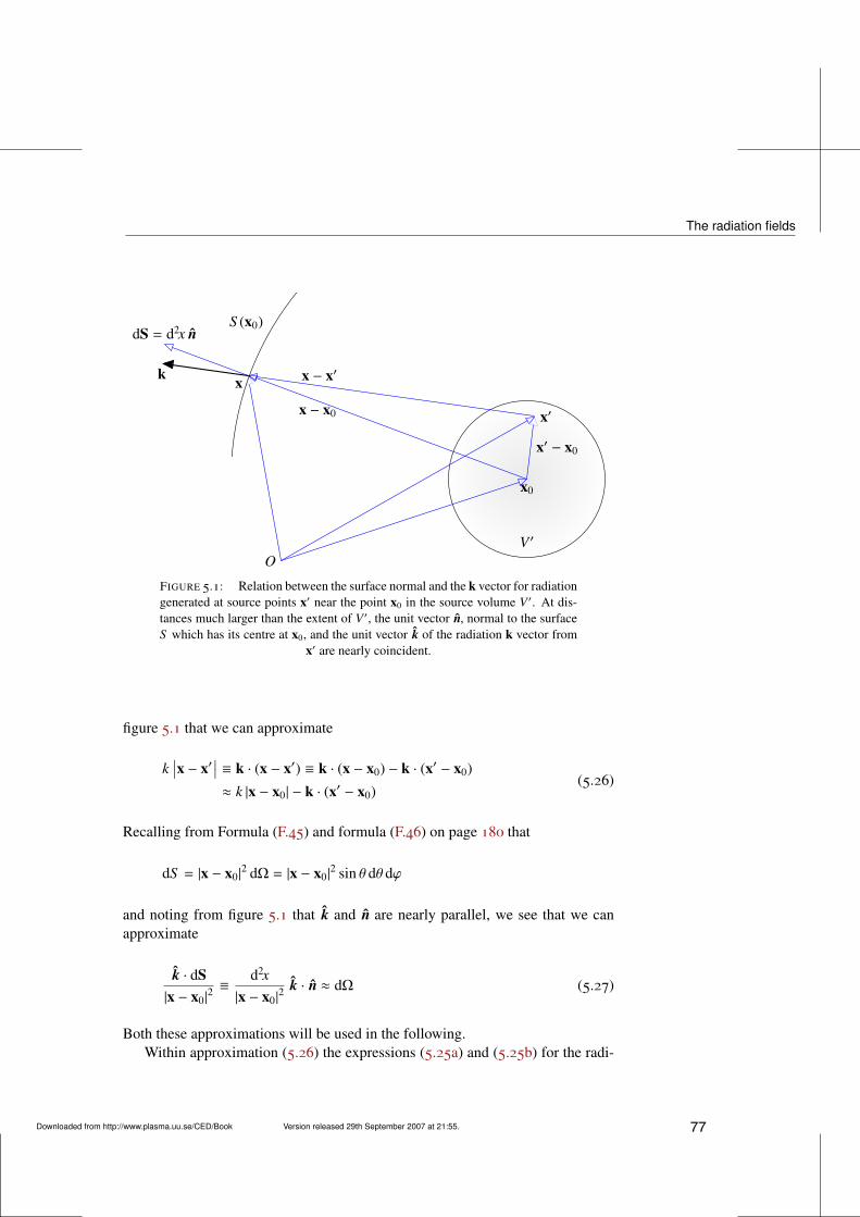
The radiation fields
V ′
O
x0
x
x − x0
dS = d2x n
x′
x − x′
S (x0)
k
x′ − x0
FIGURE 5.1: Relation between the surface normal and the k vector for radiationgenerated at source points x′ near the point x0 in the source volume V ′. At dis-tances much larger than the extent of V ′, the unit vector n, normal to the surfaceS which has its centre at x0, and the unit vector k of the radiation k vector from
x′ are nearly coincident.
figure 5.1 that we can approximate
k∣∣x − x′
∣∣ ≡ k · (x − x′) ≡ k · (x − x0) − k · (x′ − x0)
≈ k |x − x0| − k · (x′ − x0)(5.26)
Recalling from Formula (F.45) and formula (F.46) on page 180 that
dS = |x − x0|2 dΩ = |x − x0|
2 sin θ dθ dϕ
and noting from figure 5.1 that k and n are nearly parallel, we see that we canapproximate
k · dS|x − x0|
2 ≡d2x
|x − x0|2 k · n ≈ dΩ (5.27)
Both these approximations will be used in the following.Within approximation (5.26) the expressions (5.25a) and (5.25b) for the radi-
Downloaded from http://www.plasma.uu.se/CED/Book Version released 29th September 2007 at 21:55. 77
5. Electromagnetic Fields from Arbitrary Source Distributions
ation fields can be approximated as
Bradω (x) ≈ −i
µ0
4πeik|x−x0 |
∫V ′
d3x′jω(x′) × k|x − x′|
e−ik·(x′−x0)
≈ −iµ0
4πeik|x−x0 |
|x − x0|
∫V ′
d3x′ [jω(x′) × k] e−ik·(x′−x0)(5.28a)
Eradω (x) ≈ −i
14πε0c
eik|x−x0 |
∫V ′
d3x′[jω(x′) × k] × (x − x′)
|x − x′|2e−ik·(x′−x0)
≈ i1
4πε0ceik|x−x0 |
|x − x0|
(x − x0)|x − x0|
×
∫V ′
d3x′ [jω(x′) × k] e−ik·(x′−x0)
(5.28b)
I.e., if max |x′ − x0| |x − x′|, then the fields can be approximated as sphericalwaves multiplied by dimensional and angular factors, with integrals over points inthe source volume only.
5.4 Radiated energyLet us consider the energy that is carried in the radiation fields Brad, equation (5.25a),and Erad, equation (5.25b) on page 76. We have to treat signals with limited life-time and hence finite frequency bandwidth differently from monochromatic sig-nals.
5.4.1 Monochromatic signalsIf the source is strictly monochromatic, we can obtain the temporal average of theradiated power P directly, simply by averaging over one period so that
〈S〉 = 〈E ×H〉 =1
2µ0Re E × B∗ =
12µ0
Re
Eωe−iωt× (Bωe−iωt)∗
=
12µ0
Re
Eω × B∗ω e−iωteiωt = 12µ0
Re
Eω × B∗ω (5.29)
Using the far-field approximations (5.28a) and (5.28b) and the fact that 1/c =√ε0µ0 and R0 =
√µ0/ε0 according to the definition (2.26) on page 31, we obtain
〈S〉 =1
32π2 R01
|x − x0|2
∣∣∣∣∫V ′
d3x′ (jω × k)e−ik·(x′−x0)∣∣∣∣2 x − x0
|x − x0|(5.30)
78 Version released 29th September 2007 at 21:55. Downloaded from http://www.plasma.uu.se/CED/Book
Radiated energy
or, making use of (5.27) on page 77,
dPdΩ=
132π2 R0
∣∣∣∣∫V ′
d3x′ (jω × k)e−ik·(x′−x0)∣∣∣∣2 (5.31)
which is the radiated power per unit solid angle.
5.4.2 Finite bandwidth signalsA signal with finite pulse width in time (t) domain has a certain spread in fre-quency (ω) domain. To calculate the total radiated energy we need to integrateover the whole bandwidth. The total energy transmitted through a unit area is thetime integral of the Poynting vector:∫ ∞
−∞
dt S(t) =∫ ∞−∞
dt (E ×H)
=
∫ ∞−∞
dω∫ ∞−∞
dω′∫ ∞−∞
dt (Eω ×Hω′) e−i(ω+ω′)t(5.32)
If we carry out the temporal integration first and use the fact that∫ ∞−∞
dt e−i(ω+ω′)t = 2πδ(ω + ω′) (5.33)
equation (5.32) can be written [cf. Parseval’s identity]∫ ∞−∞
dt S(t) = 2π∫ ∞−∞
dω (Eω ×H−ω)
= 2π(∫ ∞
0dω (Eω ×H−ω) +
∫ 0
−∞
dω (Eω ×H−ω))
= 2π(∫ ∞
0dω (Eω ×H−ω) −
∫ −∞0
dω (Eω ×H−ω))
= 2π(∫ ∞
0dω (Eω ×H−ω) +
∫ ∞0
dω (E−ω ×Hω))
=2πµ0
∫ ∞0
dω (Eω × B−ω + E−ω × Bω)
=2πµ0
∫ ∞0
dω (Eω × B∗ω + E∗ω × Bω)
(5.34)
where the last step follows from physical requirement of real-valuedness of Eω
and Bω. We insert the Fourier transforms of the field components which dominateat large distances, i.e., the radiation fields (5.25a) and (5.25b). The result, after
Downloaded from http://www.plasma.uu.se/CED/Book Version released 29th September 2007 at 21:55. 79
5. Electromagnetic Fields from Arbitrary Source Distributions
integration over the area S of a large sphere which encloses the source volume V ′,is
U =1
4π
õ0
ε0
∮S
d2x n ·∫ ∞
0dω∣∣∣∣∫
V ′d3x′
jω × k|x − x′|
eik|x−x′ |∣∣∣∣2 k (5.35)
Inserting the approximations (5.26) and (5.27) into equation (5.35) above andalso introducing
U =∫ ∞
0dωUω (5.36)
and recalling the definition (2.26) on page 31 for the vacuum resistance R0 weobtain
dUω
dΩdω ≈
14π
R0
∣∣∣∣∫V ′
d3x′ (jω × k)e−ik·(x′−x0)∣∣∣∣2 dω (5.37)
which, at large distances, is a good approximation to the energy that is radiatedper unit solid angle dΩ in a frequency band dω. It is important to notice thatFormula (5.37) includes only source coordinates. This means that the amount ofenergy that is being radiated is independent on the distance to the source (as longas it is large).
5.5 Bibliography[1] F. HOYLE, SIR AND J. V. NARLIKAR, Lectures on Cosmology and Action at a Distance
Electrodynamics, World Scientific Publishing Co. Pte. Ltd, Singapore, New Jersey, Lon-don and Hong Kong, 1996, ISBN 9810-02-2573-3(pbk).
[2] J. D. JACKSON, Classical Electrodynamics, third ed., John Wiley & Sons, Inc.,New York, NY . . . , 1999, ISBN 0-471-30932-X.
[3] L. D. LANDAU AND E. M. LIFSHITZ, The Classical Theory of Fields, fourth revised En-glish ed., vol. 2 of Course of Theoretical Physics, Pergamon Press, Ltd., Oxford . . . , 1975,ISBN 0-08-025072-6.
[4] W. K. H. PANOFSKY AND M. PHILLIPS, Classical Electricity and Magnetism, second ed.,Addison-Wesley Publishing Company, Inc., Reading, MA . . . , 1962, ISBN 0-201-05702-6.
[5] J. A. STRATTON, Electromagnetic Theory, McGraw-Hill Book Company, Inc., NewYork, NY and London, 1953, ISBN 07-062150-0.
80 Version released 29th September 2007 at 21:55. Downloaded from http://www.plasma.uu.se/CED/Book
Downloaded from http://www.plasma.uu.se/CED/Book Version released 29th September 2007 at 21:55.
6Electromagnetic
Radiation andRadiating
Systems
In chapter 3 we were able to derive general expressions for the scalar and vectorpotentials from which we then, in chapter 5, calculated the total electric and mag-netic fields from arbitrary distributions of charge and current sources. The onlylimitation in the calculation of the fields was that the advanced potentials werediscarded.
Thus, one can, at least in principle, calculate the radiated fields, Poyntingflux, energy and other electromagnetic quantities for an arbitrary current densityFourier component and then add these Fourier components together to constructthe complete electromagnetic field at any time at any point in space. However, inpractice, it is often difficult to evaluate the source integrals unless the current hasa simple distribution in space. In the general case, one has to resort to approxima-tions. We shall consider both these situations.
6.1 Radiation from an extended source volume at restCertain radiating systems have a symmetric geometry or are in any other waysimple enough that a direct (semi-)analytic calculation of the radiated fields andenergy is possible. This is for instance the case when the radiating current flowsin a finite, conducting medium of simple geometry at rest such as in a stationaryantenna.
81
6. Electromagnetic Radiation and Radiating Systems
6.1.1 Radiation from a one-dimensional current distributionLet us apply equation (5.31) on page 79 to calculate the radiated EM power froma one-dimensional, time-varying current. Such a current can be set up by feedingthe EMF of a generator (eg., a transmitter) onto a stationary, linear, straight, thin,conducting wire across a very short gap at its centre. Due to the EMF the chargesin this thin wire of finite length L are set into motion to produce a time-varyingantenna current which is the source of the EM radiation. Linear antennas of thistype are called dipole antennas. For simplicity, we assume that the conductorresistance and the energy loss due to the electromagnetic radiation are negligible.
Choosing our coordinate system such that the x3 axis is along the antenna axis,the antenna current can be represented as j(t′, x′) = δ(x′1)δ(x′2)J(t′, x′3) x3 (mea-sured in A/m2) where J(t′, x′3) is the current (measured in A) along the antennawire. Since we can assume that the antenna wire is infinitely thin, the current mustvanish at the endpoints −L/2 and L/2 and is equal to the supplied current at themidpoint where the antenna is fed across a very short gap in the antenna wire.
For each Fourier frequency component ω0, the antenna current J(t′, x′3) can bewritten as I(x′3) exp−iω0t′ so that the antenna current density can be representedas j(t′, x′) = j0(x′) exp−iω0t′ [cf. equations (5.6) on page 70] where
j0(x′) = δ(x′1)δ(x′2)I(x′3) (6.1)
and where the spatially varying Fourier amplitude I(x′3) of the antenna currentfulfils the time-independent wave equation (Helmholtz equation)
d2Idx′23+ k2I(x′3) = 0 , I(−L/2) = I(L/2) = 0 , I(0) = I0 (6.2)
This equation has the well-known solution
I(x′3) = I0sin[k(L/2 −
∣∣x′3∣∣)]sin(kL/2)
(6.3)
where I0 is the amplitude of the antenna current (measured in A), assumed to beconstant and supplied by the generator/transmitter at the antenna feed point (inour case the midpoint of the antenna wire) and 1/ sin(kL/2) is a normalisationfactor. The antenna current forms a standing wave as indicated in figure 6.1 onpage 83.
When the antenna is short we can approximate the current distribution for-mula (6.3) by the first term in its Taylor expansion, i.e., by I0(1 − 2|x′3|/L). Fora half-wave antenna (L = λ/2 ⇔ kL = π) formula (6.3) above simplifies toI0 cos(kx′3). Hence, in the most general case of a straight, infinitely thin antennaof finite, arbitrary length L directed along the x′3 axis, the Fourier amplitude of the
82 Version released 29th September 2007 at 21:55. Downloaded from http://www.plasma.uu.se/CED/Book
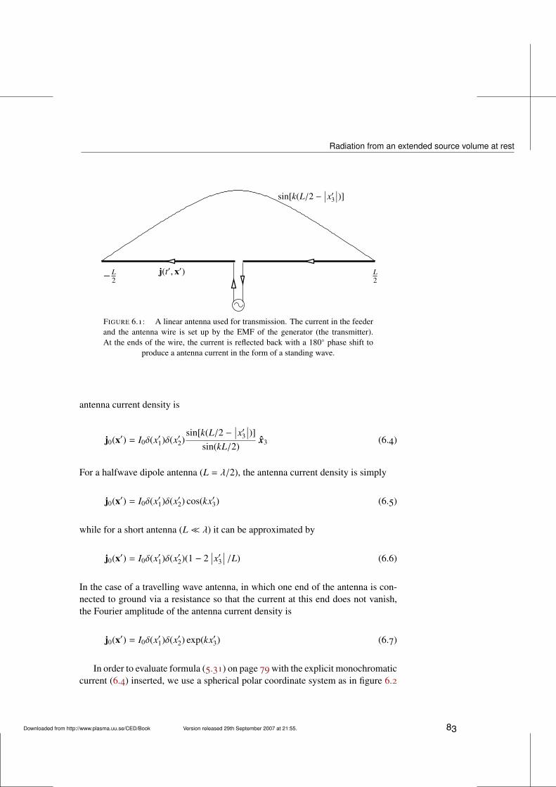
Radiation from an extended source volume at rest
j(t′, x′)− L2
sin[k(L/2 −∣∣x′3∣∣)]
L2
FIGURE 6.1: A linear antenna used for transmission. The current in the feederand the antenna wire is set up by the EMF of the generator (the transmitter).At the ends of the wire, the current is reflected back with a 180 phase shift to
produce a antenna current in the form of a standing wave.
antenna current density is
j0(x′) = I0δ(x′1)δ(x′2)sin[k(L/2 −
∣∣x′3∣∣)]sin(kL/2)
x3 (6.4)
For a halfwave dipole antenna (L = λ/2), the antenna current density is simply
j0(x′) = I0δ(x′1)δ(x′2) cos(kx′3) (6.5)
while for a short antenna (L λ) it can be approximated by
j0(x′) = I0δ(x′1)δ(x′2)(1 − 2∣∣x′3∣∣ /L) (6.6)
In the case of a travelling wave antenna, in which one end of the antenna is con-nected to ground via a resistance so that the current at this end does not vanish,the Fourier amplitude of the antenna current density is
j0(x′) = I0δ(x′1)δ(x′2) exp(kx′3) (6.7)
In order to evaluate formula (5.31) on page 79with the explicit monochromaticcurrent (6.4) inserted, we use a spherical polar coordinate system as in figure 6.2
Downloaded from http://www.plasma.uu.se/CED/Book Version released 29th September 2007 at 21:55. 83
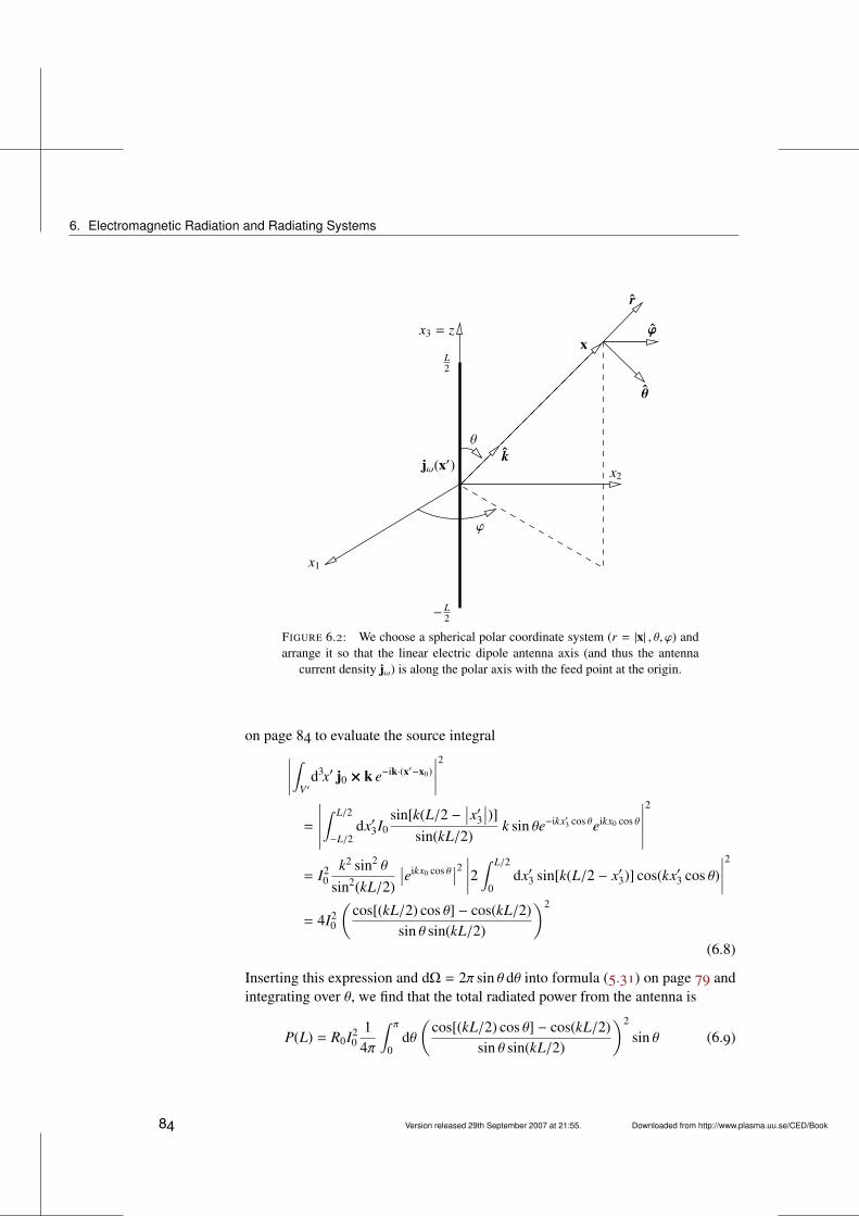
6. Electromagnetic Radiation and Radiating Systems
x3 = z
x2
x
jω(x′)
ϕ
k
x1
θ
r
θ
ϕ
L2
− L2
FIGURE 6.2: We choose a spherical polar coordinate system (r = |x| , θ, ϕ) andarrange it so that the linear electric dipole antenna axis (and thus the antenna
current density jω) is along the polar axis with the feed point at the origin.
on page 84 to evaluate the source integral∣∣∣∣∫V ′
d3x′ j0 × k e−ik·(x′−x0)∣∣∣∣2
=
∣∣∣∣∣∫ L/2
−L/2dx′3I0
sin[k(L/2 −∣∣x′3∣∣)]
sin(kL/2)k sin θe−ikx′3 cos θeikx0 cos θ
∣∣∣∣∣2
= I20
k2 sin2 θ
sin2(kL/2)
∣∣eikx0 cos θ∣∣2 ∣∣∣∣2 ∫ L/2
0dx′3 sin[k(L/2 − x′3)] cos(kx′3 cos θ)
∣∣∣∣2= 4I2
0
(cos[(kL/2) cos θ] − cos(kL/2)
sin θ sin(kL/2)
)2
(6.8)
Inserting this expression and dΩ = 2π sin θ dθ into formula (5.31) on page 79 andintegrating over θ, we find that the total radiated power from the antenna is
P(L) = R0I20
14π
∫ π
0dθ(
cos[(kL/2) cos θ] − cos(kL/2)sin θ sin(kL/2)
)2
sin θ (6.9)
84 Version released 29th September 2007 at 21:55. Downloaded from http://www.plasma.uu.se/CED/Book
Radiation from an extended source volume at rest
One can show that
limkL→0
P(L) =π
12
(Lλ
)2
R0I20 (6.10)
where λ is the vacuum wavelength.The quantity
Rrad(L) =P(L)I2eff=
P(L)12 I2
0= R0
π
6
(Lλ
)2
≈ 197(
Lλ
)2
Ω (6.11)
is called the radiation resistance. For the technologically important case of ahalf-wave antenna, i.e., for L = λ/2 or kL = π, formula (6.9) on page 84 reducesto
P(λ/2) = R0I20
14π
∫ π
0dθ
cos2(π2 cos θ
)sin θ
(6.12)
The integral in (6.12) can always be evaluated numerically. But, it can in fact alsobe evaluated analytically as follows:∫ π
0
cos2(π2 cos θ
)sin θ
dθ = [cos θ → u] =∫ 1
−1
cos2(π2 u)
1 − u2 du =[cos2
(π2
u)=
1 + cos(πu)2
]=
12
∫ 1
−1
1 + cos(πu)(1 + u)(1 − u)
du
=14
∫ 1
−1
1 + cos(πu)(1 + u)
du +14
∫ 1
−1
1 + cos(πu)(1 − u)
du
=12
∫ 1
−1
1 + cos(πu)(1 + u)
du =[1 + u→
v
π
]=
12
∫ 2π
0
1 − cos vv
dv =12
[γ + ln 2π − Ci(2π)]
≈ 1.22(6.13)
where in the last step the Euler-Mascheroni constant γ = 0.5772 . . . and the cosineintegral Ci(x) were introduced. Inserting this into the expression equation (6.12)we obtain the value Rrad(λ/2) ≈ 73 Ω.
6.1.2 Radiation from a two-dimensional current distributionAs an example of a two-dimensional current distribution we consider a circularloop antenna and calculate the radiated fields from such an antenna. We choose
Downloaded from http://www.plasma.uu.se/CED/Book Version released 29th September 2007 at 21:55. 85
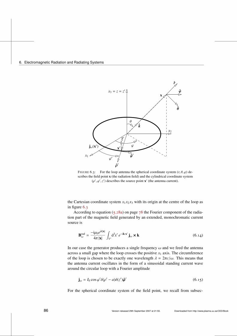
6. Electromagnetic Radiation and Radiating Systems
x2
k
ϕ
ϕ′
jω(x′)
x1
x′
ρ′
ϕ′
θ
θ
ϕx
r
x3 = z = z′
z′
FIGURE 6.3: For the loop antenna the spherical coordinate system (r, θ, ϕ) de-scribes the field point x (the radiation field) and the cylindrical coordinate system
(ρ′, ϕ′, z′) describes the source point x′ (the antenna current).
the Cartesian coordinate system x1x2x3 with its origin at the centre of the loop asin figure 6.3
According to equation (5.28a) on page 78 the Fourier component of the radia-tion part of the magnetic field generated by an extended, monochromatic currentsource is
Bradω =
−iµ0eik|x|
4π |x|
∫V ′
d3x′ e−ik·x′ jω × k (6.14)
In our case the generator produces a single frequency ω and we feed the antennaacross a small gap where the loop crosses the positive x1 axis. The circumferenceof the loop is chosen to be exactly one wavelength λ = 2πc/ω. This means thatthe antenna current oscillates in the form of a sinusoidal standing current wavearound the circular loop with a Fourier amplitude
jω = I0 cosϕ′δ(ρ′ − a)δ(z′)ϕ′ (6.15)
For the spherical coordinate system of the field point, we recall from subsec-
86 Version released 29th September 2007 at 21:55. Downloaded from http://www.plasma.uu.se/CED/Book
Radiation from an extended source volume at rest
tion F.4.1 on page 180 that the following relations between the base vectors hold:
r = sin θ cosϕx1 + sin θ sinϕx2 + cos θx3
θ = cos θ cosϕx1 + cos θ sinϕx2 − sin θx3
ϕ = − sinϕx1 + cosϕx2
and
x1 = sin θ cosϕr + cos θ cosϕθ − sinϕϕ
x2 = sin θ sinϕr + cos θ sinϕθ + cosϕϕ
x3 = cos θ r − sin θθ
With the use of the above transformations and trigonometric identities, we obtainfor the cylindrical coordinate system which describes the source:
ρ′ = cosϕ′ x1 + sinϕ′ x2
= sin θ cos(ϕ′ − ϕ)r + cos θ cos(ϕ′ − ϕ)θ + sin(ϕ′ − ϕ)ϕ(6.16)
ϕ′ = − sinϕ′ x1 + cosϕ′ x2
= − sin θ sin(ϕ′ − ϕ)r − cos θ sin(ϕ′ − ϕ)θ + cos(ϕ′ − ϕ)ϕ(6.17)
z′ = x3 = cos θ r − sin θθ (6.18)
This choice of coordinate systems means that k = k r and x′ = aρ′ so that
k · x′ = ka sin θ cos(ϕ′ − ϕ) (6.19)
and
ϕ′ × k = k[cos(ϕ′ − ϕ)θ + cos θ sin(ϕ′ − ϕ)ϕ] (6.20)
With these expressions inserted, recalling that in cylindrical coordinates d3x′ =ρ′dρ′dϕ′dz′, the source integral becomes∫
V ′d3x′ e−ik·x′ jω × k = a
∫ 2π
0dϕ′ e−ika sin θ cos(ϕ′−ϕ)I0 cosϕ′ ϕ′ × k
= I0ak∫ 2π
0e−ika sin θ cos(ϕ′−ϕ) cos(ϕ′ − ϕ) cosϕ′ dϕ′ θ
+ I0ak cos θ∫ 2π
0e−ika sin θ cos(ϕ′−ϕ) sin(ϕ′ − ϕ) cosϕ′ dϕ′ ϕ
(6.21)
Utilising the periodicity of the integrands over the integration interval [0, 2π],introducing the auxiliary integration variable ϕ′′ = ϕ′ − ϕ, and utilising standard
Downloaded from http://www.plasma.uu.se/CED/Book Version released 29th September 2007 at 21:55. 87
6. Electromagnetic Radiation and Radiating Systems
trigonometric identities, the first integral in the RHS of (6.21) can be rewritten∫ 2π
0e−ika sin θ cosϕ′′ cosϕ′′ cos(ϕ′′ + ϕ) dϕ′′
= cosϕ∫ 2π
0e−ika sin θ cosϕ′′ cos2 ϕ′′ dϕ′′ + a vanishing integral
= cosϕ∫ 2π
0e−ika sin θ cosϕ′′
(12+
12
cos 2ϕ′′)
dϕ′′
=12
cosϕ∫ 2π
0e−ika sin θ cosϕ′′ dϕ′′
+12
cosϕ∫ 2π
0e−ika sin θ cosϕ′′ cos(2ϕ′′) dϕ′′
(6.22)
Analogously, the second integral in the RHS of (6.21) can be rewritten∫ 2π
0e−ika sin θ cosϕ′′ sinϕ′′ cos(ϕ′′ + ϕ) dϕ′′
=12
sinϕ∫ 2π
0e−ika sin θ cosϕ′′ dϕ′′
−12
sinϕ∫ 2π
0e−ika sin θ cosϕ′′ cos 2ϕ′′ dϕ′′
(6.23)
As is well-known from the theory of Bessel functions,
Jn(−ξ) = (−1)nJn(ξ)
Jn(−ξ) =i−n
π
∫ π
0e−iξ cosϕ cos nϕ dϕ =
i−n
2π
∫ 2π
0e−iξ cosϕ cos nϕ dϕ
(6.24)
which means that∫ 2π
0e−ika sin θ cosϕ′′ dϕ′′ = 2πJ0(ka sin θ)∫ 2π
0e−ika sin θ cosϕ′′ cos 2ϕ′′ dϕ′′ = −2πJ2(ka sin θ)
(6.25)
Putting everything together, we find that∫V ′
d3x′ e−ik·x′ jω × k = Iθ θ + Iϕ ϕ
= I0akπ cosϕ [J0(ka sin θ) − J2(ka sin θ)] θ
+ I0akπ cos θ sinϕ [J0(ka sin θ) + J2(ka sin θ)] ϕ
(6.26)
so that, in spherical coordinates where |x| = r,
Bradω (x) =
−iµ0eikr
4πr
(Iθ θ + Iϕ ϕ
)(6.27)
88 Version released 29th September 2007 at 21:55. Downloaded from http://www.plasma.uu.se/CED/Book
Radiation from a localised source volume at rest
To obtain the desired physical magnetic field in the radiation (far) zone wemust Fourier transform back to t space and take the real part and evaluate it at theretarded time:
Brad(t, x) = Re−iµ0e(ikr−ωt′)
4πr
(Iθ θ + Iϕ ϕ
)=
µ0
4πrsin(kr − ωt′)
(Iθ θ + Iϕ ϕ
)=
I0akµ0
4rsin(kr − ωt′)
(cosϕ [J0(ka sin θ) − J2(ka sin θ)] θ
+ cos θ sinϕ [J0(ka sin θ) + J2(ka sin θ)] ϕ)
(6.28)
From this expression for the radiated B field, we can obtain the radiated E fieldwith the help of Maxwell’s equations.
6.2 Radiation from a localised source volume at restIn the general case, and when we are interested in evaluating the radiation far froma source at rest and which is localised in a small volume, we can introduce anapproximation which leads to a multipole expansion where individual terms canbe evaluated analytically. We shall use Hertz’ method to obtain this expansion.
6.2.1 The Hertz potentialLet us consider the equation of continuity, which, according to expression (1.23)on page 10, can be written
∂ρ(t, x)∂t
+ ∇ · j(t, x) = 0 (6.29)
In section 4.1.1 we introduced the electric polarisation P(t, x) such that−∇ · P = ρpol, the polarisation charge density. If we introduce a vector field π(t, x)such that
∇ · π = −ρtrue (6.30a)∂π
∂t= jtrue (6.30b)
Downloaded from http://www.plasma.uu.se/CED/Book Version released 29th September 2007 at 21:55. 89
6. Electromagnetic Radiation and Radiating Systems
and compare with equation (6.29) on page 89, we see that π(t, x) satisfies thisequation of continuity. Furthermore, if we compare with the electric polarisation[cf. equation (4.9) on page 59], we see that the quantity π is related to the ‘true’charges in the same way as P is related to polarised charge, namely as a dipolemoment density. The quantity π is referred to as the polarisation vector since,formally, it treats also the ‘true’ (free) charges as polarisation charges so that
∇ · E =ρtrue + ρpol
ε0=−∇ · π − ∇ · P
ε0(6.31)
We introduce a further potential Πe with the following property
∇ ·Πe = −φ (6.32a)1c2
∂Πe
∂t= A (6.32b)
where φ and A are the electromagnetic scalar and vector potentials, respectively.As we see, Πe acts as a ‘super-potential’ in the sense that it is a potential fromwhich we can obtain other potentials. It is called the Hertz’ vector or polarisationpotential. Requiring that the scalar and vector potentials φ and A, respectively,fulfil their inhomogeneous wave equations, one finds, using (6.30) and (6.32),that Hertz’ vector must satisfy the inhomogeneous wave equation
2Πe =1c2
∂2
∂t2Πe − ∇2Πe =
π
ε0(6.33)
This equation is of the same type as equation (3.17) on page 47, and has there-fore the retarded solution
Πe(t, x) =1
4πε0
∫V ′
d3x′π(t′ret, x′)|x − x′|
(6.34)
with Fourier components
Πeω(x) =
14πε0
∫V ′
d3x′πω(x′)eik|x−x′ |
|x − x′|(6.35)
If we introduce the help vector C such that
C = ∇ ×Πe (6.36)
we see that we can calculate the magnetic and electric fields, respectively, as fol-lows
B =1c2
∂C∂t
(6.37a)
E = ∇ × C (6.37b)
90 Version released 29th September 2007 at 21:55. Downloaded from http://www.plasma.uu.se/CED/Book
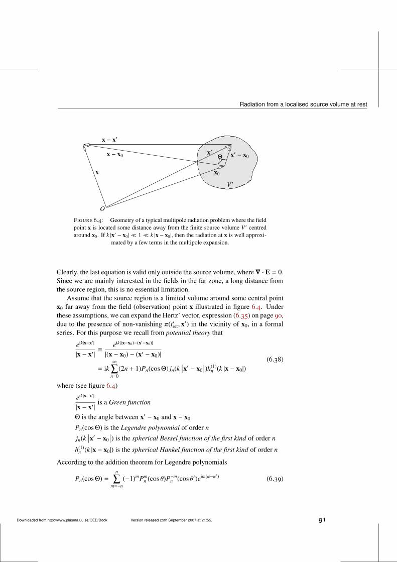
Radiation from a localised source volume at rest
x − x′
x x0
V ′
O
Θx′x − x0 x′ − x0
FIGURE 6.4: Geometry of a typical multipole radiation problem where the fieldpoint x is located some distance away from the finite source volume V ′ centredaround x0. If k |x′ − x0| 1 k |x − x0|, then the radiation at x is well approxi-
mated by a few terms in the multipole expansion.
Clearly, the last equation is valid only outside the source volume, where∇ · E = 0.Since we are mainly interested in the fields in the far zone, a long distance fromthe source region, this is no essential limitation.
Assume that the source region is a limited volume around some central pointx0 far away from the field (observation) point x illustrated in figure 6.4. Underthese assumptions, we can expand the Hertz’ vector, expression (6.35) on page 90,due to the presence of non-vanishing π(t′ret, x′) in the vicinity of x0, in a formalseries. For this purpose we recall from potential theory that
eik|x−x′ |
|x − x′|≡
eik|(x−x0)−(x′−x0)|
|(x − x0) − (x′ − x0)|
= ik∞
∑n=0
(2n + 1)Pn(cosΘ) jn(k∣∣x′ − x0
∣∣)h(1)n (k |x − x0|)
(6.38)
where (see figure 6.4)
eik|x−x′ |
|x − x′|is a Green function
Θ is the angle between x′ − x0 and x − x0
Pn(cosΘ) is the Legendre polynomial of order n
jn(k∣∣x′ − x0
∣∣) is the spherical Bessel function of the first kind of order n
h(1)n (k |x − x0|) is the spherical Hankel function of the first kind of order n
According to the addition theorem for Legendre polynomials
Pn(cosΘ) =n
∑m=−n
(−1)mPmn (cos θ)P−m
n (cos θ′)eim(ϕ−ϕ′) (6.39)
Downloaded from http://www.plasma.uu.se/CED/Book Version released 29th September 2007 at 21:55. 91
6. Electromagnetic Radiation and Radiating Systems
where Pmn is an associated Legendre polynomial and, in spherical polar coordi-
nates,
x′ − x0 = (∣∣x′ − x0
∣∣ , θ′, ϕ′) (6.40a)
x − x0 = (|x − x0| , θ, ϕ) (6.40b)
Inserting equation (6.38) on page 91, together with formula (6.39) on page 91,into equation (6.35) on page 90, we can in a formally exact way expand the Fouriercomponent of the Hertz’ vector as
Πeω =
ik4πε0
∞
∑n=0
n
∑m=−n
(2n + 1)(−1)mh(1)n (k |x − x0|) Pm
n (cos θ) eimϕ
×
∫V ′
d3x′ πω(x′) jn(k∣∣x′ − x0
∣∣) P−mn (cos θ′) e−imϕ′
(6.41)
We notice that there is no dependence on x − x0 inside the integral; the integrandis only dependent on the relative source vector x′ − x0.
We are interested in the case where the field point is many wavelengths awayfrom the well-localised sources, i.e., when the following inequalities
k∣∣x′ − x0
∣∣ 1 k |x − x0| (6.42)
hold. Then we may to a good approximation replace h(1)n with the first term in its
asymptotic expansion:
h(1)n (k |x − x0|) ≈ (−i)n+1 eik|x−x0 |
k |x − x0|(6.43)
and replace jn with the first term in its power series expansion:
jn(k∣∣x′ − x0
∣∣) ≈ 2nn!(2n + 1)!
(k∣∣x′ − x0
∣∣)n (6.44)
Inserting these expansions into equation (6.41), we obtain the multipole expansionof the Fourier component of the Hertz’ vector
Πeω ≈
∞
∑n=0Πeω
(n) (6.45a)
where
Πeω
(n) = (−i)n 14πε0
eik|x−x0 |
|x − x0|
2nn!(2n)!
∫V ′
d3x′ πω(x′) (k∣∣x′ − x0
∣∣)n Pn(cosΘ)
(6.45b)
92 Version released 29th September 2007 at 21:55. Downloaded from http://www.plasma.uu.se/CED/Book
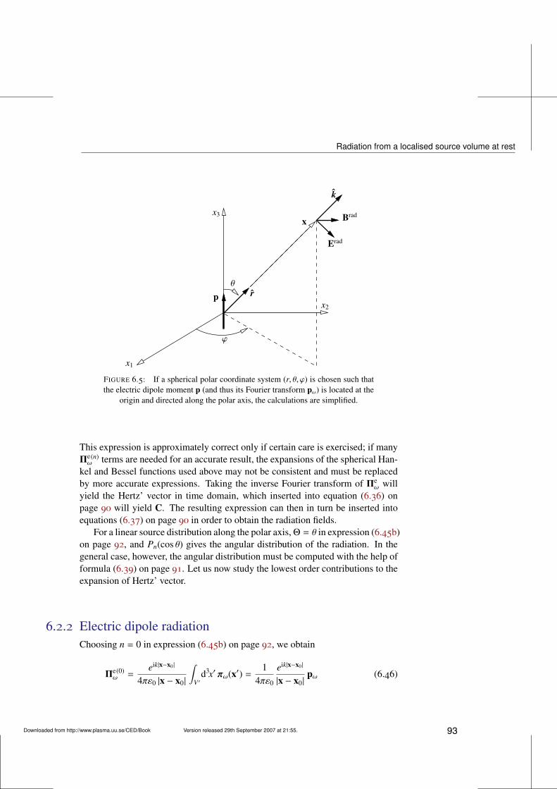
Radiation from a localised source volume at rest
Erad
x2
ϕ
r
x
k
Bradx3
p
x1
θ
FIGURE 6.5: If a spherical polar coordinate system (r, θ, ϕ) is chosen such thatthe electric dipole moment p (and thus its Fourier transform pω) is located at the
origin and directed along the polar axis, the calculations are simplified.
This expression is approximately correct only if certain care is exercised; if manyΠeω
(n) terms are needed for an accurate result, the expansions of the spherical Han-kel and Bessel functions used above may not be consistent and must be replacedby more accurate expressions. Taking the inverse Fourier transform of Πe
ω willyield the Hertz’ vector in time domain, which inserted into equation (6.36) onpage 90 will yield C. The resulting expression can then in turn be inserted intoequations (6.37) on page 90 in order to obtain the radiation fields.
For a linear source distribution along the polar axis,Θ = θ in expression (6.45b)on page 92, and Pn(cos θ) gives the angular distribution of the radiation. In thegeneral case, however, the angular distribution must be computed with the help offormula (6.39) on page 91. Let us now study the lowest order contributions to theexpansion of Hertz’ vector.
6.2.2 Electric dipole radiationChoosing n = 0 in expression (6.45b) on page 92, we obtain
Πeω
(0) =eik|x−x0 |
4πε0 |x − x0|
∫V ′
d3x′ πω(x′) =1
4πε0
eik|x−x0 |
|x − x0|pω (6.46)
Downloaded from http://www.plasma.uu.se/CED/Book Version released 29th September 2007 at 21:55. 93
6. Electromagnetic Radiation and Radiating Systems
Since π represents a dipole moment density for the ‘true’ charges (in the samevein as P does so for the polarised charges), pω =
∫V ′d
3x′ πω(x′) is the Fouriercomponent of the electric dipole moment
p(t, x0) =∫
V ′d3x′ π(t′, x′) =
∫V ′
d3x′ (x′ − x0)ρ(t′, x′) (6.47)
[cf. equation (4.2) on page 58 which describes the static dipole moment]. If aspherical coordinate system is chosen with its polar axis along pω as in figure 6.5on page 93, the components of Πe
ω(0) are
Πer
def≡ Πe
ω(0) · r =
14πε0
eik|x−x0 |
|x − x0|pω cos θ (6.48a)
Πeθ
def≡ Πe
ω(0) · θ = −
14πε0
eik|x−x0 |
|x − x0|pω sin θ (6.48b)
Πeϕ
def≡ Πe
ω(0) · ϕ = 0 (6.48c)
Evaluating formula (6.36) on page 90 for the help vector C, with the spheri-cally polar components (6.48) of Πe
ω(0) inserted, we obtain
Cω = C(0)ω,ϕ ϕ =
14πε0
(1
|x − x0|− ik
)eik|x−x0 |
|x − x0|pω sin θ ϕ (6.49)
Applying this to equations (6.37) on page 90, we obtain directly the Fourier com-ponents of the fields
Bω = −iωµ0
4π
(1
|x − x0|− ik
)eik|x−x0 |
|x − x0|pω sin θ ϕ (6.50a)
Eω =1
4πε0
[2(
1|x − x0|
2 −ik
|x − x0|
)cos θ
x − x0
|x − x0|
+
(1
|x − x0|2 −
ik|x − x0|
− k2)
sin θ θ]
eik|x−x0 |
|x − x0|pω
(6.50b)
Keeping only those parts of the fields which dominate at large distances (theradiation fields) and recalling that the wave vector k = k(x − x0)/ |x − x0| wherek = ω/c, we can now write down the Fourier components of the radiation parts ofthe magnetic and electric fields from the dipole:
Bradω = −
ωµ0
4πeik|x−x0 |
|x − x0|pωk sin θ ϕ = −
ωµ0
4πeik|x−x0 |
|x − x0|(pω × k) (6.51a)
Eradω = −
14πε0
eik|x−x0 |
|x − x0|pωk2 sin θ θ = −
14πε0
eik|x−x0 |
|x − x0|[(pω × k) × k] (6.51b)
These fields constitute the electric dipole radiation, also known as E1 radiation.
94 Version released 29th September 2007 at 21:55. Downloaded from http://www.plasma.uu.se/CED/Book
Radiation from a localised source volume at rest
6.2.3 Magnetic dipole radiationThe next term in the expression (6.45b) on page 92 for the expansion of the Fouriertransform of the Hertz’ vector is for n = 1:
Πeω
(1) = −ieik|x−x0 |
4πε0 |x − x0|
∫V ′
d3x′ k∣∣x′ − x0
∣∣πω(x′) cosΘ
= −ik1
4πε0
eik|x−x0 |
|x − x0|2
∫V ′
d3x′ [(x − x0) · (x′ − x0)]πω(x′)(6.52)
Here, the term [(x − x0) · (x′ − x0)]πω(x′) can be rewritten
[(x − x0) · (x′ − x0)]πω(x′) = (xi − x0,i)(x′i − x0,i)πω(x′) (6.53)
and introducing
ηi = xi − x0,i (6.54a)
η′i = x′i − x0,i (6.54b)
the jth component of the integrand in Πeω
(1) can be broken up into
[(x − x0) · (x′ − x0)]πω(x′) j =12ηi(πω, jη
′i + πω,iη
′j
)+
12ηi(πω, jη
′i − πω,iη
′j
) (6.55)
i.e., as the sum of two parts, the first being symmetric and the second antisymmet-ric in the indices i, j. We note that the antisymmetric part can be written as
12ηi(πω, jη
′i − πω,iη
′j
)=
12
[πω, j(ηiη′i) − η
′j(ηiπω,i)]
=12
[πω(η · η′) − η′(η · πω)] j
=12
(x − x0) × [πω × (x′ − x0)]
j
(6.56)
The utilisation of equations (6.30) on page 89, and the fact that we are consid-ering a single Fourier component,
π(t, x) = πωe−iωt (6.57)
allow us to express πω in jω as
πω = ijωω
(6.58)
Downloaded from http://www.plasma.uu.se/CED/Book Version released 29th September 2007 at 21:55. 95
6. Electromagnetic Radiation and Radiating Systems
Hence, we can write the antisymmetric part of the integral in formula (6.52) onpage 95 as
12
(x − x0) ×∫
V ′d3x′ πω(x′) × (x′ − x0)
= i1
2ω(x − x0) ×
∫V ′
d3x′ jω(x′) × (x′ − x0)
= −i1ω
(x − x0) ×mω
(6.59)
where we introduced the Fourier transform of the magnetic dipole moment
mω =12
∫V ′
d3x′ (x′ − x0) × jω(x′) (6.60)
The final result is that the antisymmetric, magnetic dipole, part ofΠeω
(1) can bewritten
Πe,antisymω
(1)= −
k4πε0ω
eik|x−x0 |
|x − x0|2 (x − x0) ×mω (6.61)
In analogy with the electric dipole case, we insert this expression into equa-tion (6.36) on page 90 to evaluate C, with which equations (6.37) on page 90then gives the B and E fields. Discarding, as before, all terms belonging to thenear fields and transition fields and keeping only the terms that dominate at largedistances, we obtain
Bradω (x) = −
µ0
4πeik|x−x0 |
|x − x0|(mω × k) × k (6.62a)
Eradω (x) =
k4πε0c
eik|x−x0 |
|x − x0|mω × k (6.62b)
which are the fields of the magnetic dipole radiation (M1 radiation).
6.2.4 Electric quadrupole radiationThe symmetric part Πe,sym
ω(1) of the n = 1 contribution in the equation (6.45b) on
page 92 for the expansion of the Hertz’ vector can be expressed in terms of theelectric quadrupole tensor, which is defined in accordance with equation (4.3) onpage 58:
Q(t, x0) =∫
V ′d3x′ (x′ − x0)(x′ − x0)ρ(t′ret, x
′) (6.63)
96 Version released 29th September 2007 at 21:55. Downloaded from http://www.plasma.uu.se/CED/Book
Radiation from a localised charge in arbitrary motion
Again we use this expression in equation (6.36) on page 90 to calculate the fieldsvia equations (6.37) on page 90. Tedious, but fairly straightforward algebra (whichwe will not present here), yields the resulting fields. The radiation components ofthe fields in the far field zone (wave zone) are given by
Bradω (x) =
iµ0ω
8πeik|x−x0 |
|x − x0|(k · Qω) × k (6.64a)
Eradω (x) =
i8πε0
eik|x−x0 |
|x − x0|[(k · Qω) × k] × k (6.64b)
This type of radiation is called electric quadrupole radiation or E2 radiation.
6.3 Radiation from a localised charge in arbitrary mo-tionThe derivation of the radiation fields for the case of the source moving relativeto the observer is considerably more complicated than the stationary cases stud-ied above. In order to handle this non-stationary situation, we use the retardedpotentials (3.34) on page 50 in chapter 3
φ(t, x) =1
4πε0
∫V ′
d3x′ρ(t′ret, x′)|x − x′|
(6.65a)
A(t, x) =µ0
4π
∫V ′
d3x′j(t′ret, x′)|x − x′|
(6.65b)
and consider a source region with such a limited spatial extent that the chargesand currents are well localised. Specifically, we consider a charge q′, for instancean electron, which, classically, can be thought of as a localised, unstructured andrigid ‘charge distribution’ with a small, finite radius. The part of this ‘chargedistribution’ dq′ which we are considering is located in dV ′ = d3x′ in the sphere infigure 6.6 on page 98. Since we assume that the electron (or any other other similarelectric charge) moves with a velocity v whose direction is arbitrary and whosemagnitude can even be comparable to the speed of light, we cannot say that thecharge and current to be used in (6.65) is
∫V ′d
3x′ ρ(t′ret, x′) and∫
V ′d3x′ vρ(t′ret, x′),
respectively, because in the finite time interval during which the observed signalis generated, part of the charge distribution will ‘leak’ out of the volume elementd3x′.
Downloaded from http://www.plasma.uu.se/CED/Book Version released 29th September 2007 at 21:55. 97
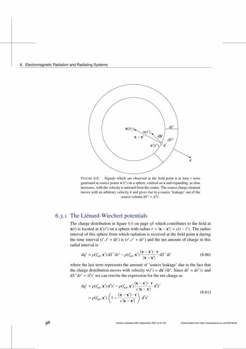
6. Electromagnetic Radiation and Radiating Systems
v(t′)
x′(t′)
dS′dV ′
dr′x(t)
q′
x − x′
c
FIGURE 6.6: Signals which are observed at the field point x at time t weregenerated at source points x′(t′) on a sphere, centred on x and expanding, as timeincreases, with the velocity c outward from the centre. The source charge elementmoves with an arbitrary velocity v and gives rise to a source ‘leakage’ out of the
source volume dV ′ = d3x′.
6.3.1 The Liénard-Wiechert potentialsThe charge distribution in figure 6.6 on page 98 which contributes to the field atx(t) is located at x′(t′) on a sphere with radius r = |x − x′| = c(t − t′). The radiusinterval of this sphere from which radiation is received at the field point x duringthe time interval (t′, t′ + dt′) is (r′, r′ + dr′) and the net amount of charge in thisradial interval is
dq′ = ρ(t′ret, x′) dS ′ dr′ − ρ(t′ret, x
′)(x − x′) · v|x − x′|
dS ′ dt′ (6.66)
where the last term represents the amount of ‘source leakage’ due to the fact thatthe charge distribution moves with velocity v(t′) = dx′/dt′. Since dt′ = dr′/c anddS ′ dr′ = d3x′ we can rewrite the expression for the net charge as
dq′ = ρ(t′ret, x′) d3x′ − ρ(t′ret, x
′)(x − x′) · vc |x − x′|
d3x′
= ρ(t′ret, x′)(
1 −(x − x′) · vc |x − x′|
)d3x′
(6.67)
98 Version released 29th September 2007 at 21:55. Downloaded from http://www.plasma.uu.se/CED/Book
Radiation from a localised charge in arbitrary motion
or
ρ(t′ret, x′) d3x′ =
dq′
1 − (x−x′)·vc|x−x′ |
(6.68)
which leads to the expression
ρ(t′ret, x′)|x − x′|
d3x′ =dq′
|x − x′| − (x−x′)·vc
(6.69)
This is the expression to be used in the formulae (6.65) on page 97 for the retardedpotentials. The result is (recall that j = ρv)
φ(t, x) =1
4πε0
∫ dq′
|x − x′| − (x−x′)·vc
(6.70a)
A(t, x) =µ0
4π
∫ v dq′
|x − x′| − (x−x′)·vc
(6.70b)
For a sufficiently small and well localised charge distribution we can, assumingthat the integrands do not change sign in the integration volume, use the meanvalue theorem to evaluate these expressions to become
φ(t, x) =1
4πε0
1|x − x′| − (x−x′)·v
c
∫V ′
d3x′ dq′ =q′
4πε0
1s
(6.71a)
A(t, x) =1
4πε0c2
v|x − x′| − (x−x′)·v
c
∫V ′
d3x′ dq′ =q′
4πε0c2
vs=
vc2 φ(t, x)
(6.71b)
where
s = s(t′, x) =∣∣x − x′(t′)
∣∣ − [x − x′(t′)] · v(t′)c
(6.72a)
=∣∣x − x′(t′)
∣∣ (1 −x − x′(t′)|x − x′(t′)|
·v(t′)
c
)(6.72b)
= [x − x′(t′)] ·(
x − x′(t′)|x − x′(t′)|
−v(t′)
c
)(6.72c)
is the retarded relative distance. The potentials (6.71) are precisely the Liénard-Wiechert potentials which will be derived in section 7.3.2 on page 148 by using arelativistically covariant formalism.
It should be noted that in the complicated derivation presented above, the ob-server is in a coordinate system which has an ‘absolute’ meaning and the velocityv is that of the localised charge q′, whereas, as we shall see later, in the covari-ant derivation, two reference frames of equal standing are moving relative to eachother with v.
Downloaded from http://www.plasma.uu.se/CED/Book Version released 29th September 2007 at 21:55. 99
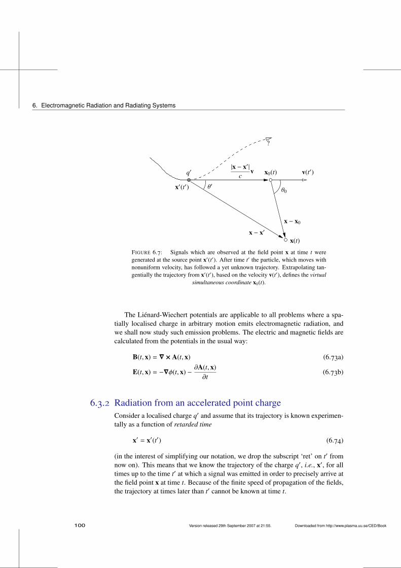
6. Electromagnetic Radiation and Radiating Systems
|x − x′|c
v
x(t)
v(t′)x0(t)
x′(t′)
x − x′x − x0
q′
θ′ θ0
?
FIGURE 6.7: Signals which are observed at the field point x at time t weregenerated at the source point x′(t′). After time t′ the particle, which moves withnonuniform velocity, has followed a yet unknown trajectory. Extrapolating tan-gentially the trajectory from x′(t′), based on the velocity v(t′), defines the virtual
simultaneous coordinate x0(t).
The Liénard-Wiechert potentials are applicable to all problems where a spa-tially localised charge in arbitrary motion emits electromagnetic radiation, andwe shall now study such emission problems. The electric and magnetic fields arecalculated from the potentials in the usual way:
B(t, x) = ∇ × A(t, x) (6.73a)
E(t, x) = −∇φ(t, x) −∂A(t, x)∂t
(6.73b)
6.3.2 Radiation from an accelerated point chargeConsider a localised charge q′ and assume that its trajectory is known experimen-tally as a function of retarded time
x′ = x′(t′) (6.74)
(in the interest of simplifying our notation, we drop the subscript ‘ret’ on t′ fromnow on). This means that we know the trajectory of the charge q′, i.e., x′, for alltimes up to the time t′ at which a signal was emitted in order to precisely arrive atthe field point x at time t. Because of the finite speed of propagation of the fields,the trajectory at times later than t′ cannot be known at time t.
100 Version released 29th September 2007 at 21:55. Downloaded from http://www.plasma.uu.se/CED/Book
Radiation from a localised charge in arbitrary motion
The retarded velocity and acceleration at time t′ are given by
v(t′) =dx′
dt′(6.75a)
a(t′) = v(t′) =dvdt′=
d2x′
dt′2(6.75b)
As for the charge coordinate x′ itself, we have in general no knowledge of thevelocity and acceleration at times later than t′, and definitely not at the time ofobservation t! If we choose the field point x as fixed, application of (6.75) to therelative vector x − x′ yields
ddt′
[x − x′(t′)] = −v(t′) (6.76a)
d2
dt′2[x − x′(t′)] = −v(t′) (6.76b)
The retarded time t′ can, at least in principle, be calculated from the implicitrelation
t′ = t′(t, x) = t −|x − x′(t′)|
c(6.77)
and we shall see later how this relation can be taken into account in the calcula-tions.
According to formulae (6.73) on page 100 the electric and magnetic fields aredetermined via differentiation of the retarded potentials at the observation time tand at the observation point x. In these formulae the unprimed ∇, i.e., the spatialderivative differentiation operator ∇ = xi∂/∂xi means that we differentiate withrespect to the coordinates x = (x1, x2, x3) while keeping t fixed, and the unprimedtime derivative operator ∂/∂t means that we differentiate with respect to t whilekeeping x fixed. But the Liénard-Wiechert potentials φ and A, equations (6.71) onpage 99, are expressed in the charge velocity v(t′) given by equation (6.75a) aboveand the retarded relative distance s(t′, x) given by equation (6.72) on page 99.This means that the expressions for the potentials φ and A contain terms whichare expressed explicitly in t′, which in turn is expressed implicitly in t via equa-tion (6.77) above. Despite this complication it is possible, as we shall see below,to determine the electric and magnetic fields and associated quantities at the timeof observation t. To this end, we need to investigate carefully the action of differ-entiation on the potentials.
The differential operator methodWe introduce the convention that a differential operator embraced by parentheseswith an index x or t means that the operator in question is applied at constant x
Downloaded from http://www.plasma.uu.se/CED/Book Version released 29th September 2007 at 21:55. 101
6. Electromagnetic Radiation and Radiating Systems
and t, respectively. With this convention, we find that(∂
∂t′
)x
∣∣x − x′(t′)∣∣ = x − x′
|x − x′|·
(∂
∂t′
)x
(x − x′(t′)
)= −
(x − x′) · v(t′)|x − x′|
(6.78)
Furthermore, by applying the operator (∂/∂t)x to equation (6.77) on page 101 wefind that(
∂t′
∂t
)x= 1 −
(∂
∂t
)x
|x − x′(t′(t, x))|c
= 1 −[(
∂
∂t′
)x
|x − x′|c
](∂t′
∂t
)x
= 1 +(x − x′) · v(t′)
c |x − x′|
(∂t′
∂t
)x
(6.79)
This is an algebraic equation in (∂t′/∂t)x which we can solve to obtain(∂t′
∂t
)x=
|x − x′||x − x′| − (x − x′) · v(t′)/c
=|x − x′|
s(6.80)
where s = s(t′, x) is the retarded relative distance given by equation (6.72) onpage 99. Making use of equation (6.80), we obtain the following useful operatoridentity(
∂
∂t
)x=
(∂t′
∂t
)x
(∂
∂t′
)x=|x − x′|
s
(∂
∂t′
)x
(6.81)
Likewise, by applying (∇)t to equation (6.77) on page 101 we obtain
(∇)t t′ = −(∇)t|x − x′(t′(t, x))|
c= −
x − x′
c |x − x′|· (∇)t(x − x′)
= −x − x′
c |x − x′|+
(x − x′) · v(t′)c |x − x′|
(∇)t t′(6.82)
This is an algebraic equation in (∇)t t′ with the solution
(∇)tt′ = −x − x′
cs(6.83)
which gives the following operator relation when (∇)t is acting on an arbitraryfunction of t′ and x:
(∇)t =[(∇)tt′
]( ∂
∂t′
)x+ (∇)t′ = −
x − x′
cs
(∂
∂t′
)x+ (∇)t′ (6.84)
102 Version released 29th September 2007 at 21:55. Downloaded from http://www.plasma.uu.se/CED/Book
Radiation from a localised charge in arbitrary motion
With the help of the rules (6.84) and (6.81) we are now able to replace t by t′ inthe operations which we need to perform. We find, for instance, that
∇φ ≡ (∇φ)t = ∇
(1
4πε0
q′
s
)= −
q′
4πε0s2
[x − x′
|x − x′|−
v(t′)c−
x − x′
cs
(∂s∂t′
)x
] (6.85a)
∂A∂t≡
(∂A∂t
)x=∂
∂t
(µ0
4πq′v(t′)
s
)x
=q′
4πε0c2s3
[∣∣x − x′∣∣ sv(t′) −
∣∣x − x′∣∣ v(t′)
(∂s∂t′
)x
] (6.85b)
Utilising these relations in the calculation of the E field from the Liénard-Wiechertpotentials, equations (6.71) on page 99, we obtain
E(t, x) = −∇φ(t, x) −∂
∂tA(t, x)
=q′
4πε0s2(t′, x)
[[x − x′(t′)] − |x − x′(t′)| v(t′)/c
|x − x′(t′)|
−[x − x′(t′)] − |x − x′(t′)| v(t′)/c
cs(t′, x)
(∂s(t′, x)∂t′
)x−|x − x′(t′)| v(t′)
c2
](6.86)
Starting from expression (6.72a) on page 99 for the retarded relative distances(t′, x), we see that we can evaluate (∂s/∂t′)x in the following way
(∂s∂t′
)x=
(∂
∂t′
)x
(∣∣x − x′∣∣ − (x − x′) · v(t′)
c
)=
∂
∂t′∣∣x − x′(t′)
∣∣ − 1c
(∂[x − x′(t′)]
∂t′· v(t′) + [x − x′(t′)] ·
∂v(t′)∂t′
)= −
(x − x′) · v(t′)|x − x′|
+v2(t′)
c−
(x − x′) · v(t′)c
(6.87)
where equation (6.78) on page 102 and equations (6.75) on page 101, respectively,were used. Hence, the electric field generated by an arbitrarily moving charged
Downloaded from http://www.plasma.uu.se/CED/Book Version released 29th September 2007 at 21:55. 103
6. Electromagnetic Radiation and Radiating Systems
particle at x′(t′) is given by the expression
E(t, x) =q′
4πε0s3(t′, x)
([x − x′(t′)] −
|x − x′(t′)| v(t′)c
)(1 −
v2(t′)c2
)︸ ︷︷ ︸
Coulomb field when v→ 0
+q′
4πε0s3(t′, x)
x − x′(t′)
c2 ×
[([x − x′(t′)] −
|x − x′(t′)| v(t′)c
)× v(t′)
]︸ ︷︷ ︸
Radiation (acceleration) field(6.88)
The first part of the field, the velocity field, tends to the ordinary Coulomb fieldwhen v→ 0 and does not contribute to the radiation. The second part of the field,the acceleration field, is radiated into the far zone and is therefore also called theradiation field.
From figure 6.7 on page 100 we see that the position the charged particlewould have had if at t′ all external forces would have been switched off so thatthe trajectory from then on would have been a straight line in the direction of thetangent at x′(t′) is x0(t), the virtual simultaneous coordinate. During the arbitrarymotion, we interpret x − x0(t) as the coordinate of the field point x relative to thevirtual simultaneous coordinate x0(t). Since the time it takes for a signal to prop-agate (in the assumed vacuum) from x′(t′) to x is |x − x′| /c, this relative vector isgiven by
x − x0(t) = x − x′(t′) −|x − x′(t′)| v(t′)
c(6.89)
This allows us to rewrite equation (6.88) above in the following way
E(t, x) =q′
4πε0s3
[(x − x0)
(1 −
v2
c2
)+ (x − x′) ×
(x − x0) × vc2
](6.90)
In a similar manner we can compute the magnetic field:
B(t, x) = ∇ × A(t, x) ≡ (∇)t × A = (∇)t′ × A −x − x′
cs×
(∂
∂t′
)x
A
= −q′
4πε0c2s2
x − x′
|x − x′|× v −
x − x′
c |x − x′|×
(∂A∂t
)x
(6.91)
where we made use of equation (6.71) on page 99 and formula (6.81) on page 102.But, according to (6.85a),
x − x′
c |x − x′|× (∇)tφ =
q′
4πε0c2s2
x − x′
|x − x′|× v (6.92)
104 Version released 29th September 2007 at 21:55. Downloaded from http://www.plasma.uu.se/CED/Book
Radiation from a localised charge in arbitrary motion
so that
B(t, x) =x − x′
c |x − x′|×
[−(∇φ)t −
(∂A∂t
)x
]=
x − x′
c |x − x′|× E(t, x)
(6.93)
The radiation part of the electric field is obtained from the acceleration field informula (6.88) on page 104 as
Erad(t, x) = lim|x−x′ |→∞
E(t, x)
=q′
4πε0c2s3 (x − x′) ×[(
(x − x′) −|x − x′| v
c
)× v]
=q′
4πε0c2s3 [x − x′(t′)] × [x − x0(t)] × v(t′)
(6.94)
where in the last step we again used formula (6.89) on page 104. Using thisformula and formula (6.93), the radiation part of the magnetic field can be written
Brad(t, x) =x − x′
c |x − x′|× Erad(t, x) (6.95)
The direct methodAn alternative to the differential operator transformation technique just describedis to try to express all quantities in the potentials directly in t and x. An exampleof such a quantity is the retarded relative distance s(t′, x). According to equa-tion (6.72) on page 99, the square of this retarded relative distance can be written
s2(t′, x) =∣∣x − x′(t′)
∣∣2 − 2∣∣x − x′(t′)
∣∣ [x − x′(t′)] · v(t′)c
(6.96)
+
([x − x′(t′)] · v(t′)
c
)2
(6.97)
If we use the following handy identity((x − x′) · v
c
)2
+
((x − x′) × v
c
)2
=|x − x′|2 v2
c2 cos2 θ′ +|x − x′|2 v2
c2 sin2 θ′
=|x − x′|2 v2
c2 (cos2 θ′ + sin2 θ′) =|x − x′|2 v2
c2
(6.98)
Downloaded from http://www.plasma.uu.se/CED/Book Version released 29th September 2007 at 21:55. 105
6. Electromagnetic Radiation and Radiating Systems
we find that((x − x′) · v
c
)2
=|x − x′|2 v2
c2 −
((x − x′) × v
c
)2
(6.99)
Furthermore, from equation (6.89) on page 104, we obtain the following identity:
[x − x′(t′)] × v = [x − x0(t)] × v (6.100)
which, when inserted into equation (6.99) above, yields the relation((x − x′) · v
c
)2
=|x − x′|2 v2
c2 −
((x − x0) × v
c
)2
(6.101)
Inserting the above into expression (6.96) on page 105 for s2, this expressionbecomes
s2 =∣∣x − x′
∣∣2 − 2∣∣x − x′
∣∣ (x − x′) · vc
+|x − x′|2 v2
c2 −
((x − x0) × v
c
)2
=
((x − x′) −
|x − x′| vc
)2
−
((x − x0) × v
c
)2
= (x − x0)2 −
((x − x0) × v
c
)2
≡ |x − x0(t)|2 −(
[x − x0(t)] × v(t′)c
)2
(6.102)
where in the penultimate step we used equation (6.89) on page 104.What we have just demonstrated is that if the particle velocity at time t can be
calculated or projected from its value at the retarded time t′, the retarded distances in the Liénard-Wiechert potentials (6.71) can be expressed in terms of the virtualsimultaneous coordinate x0(t), viz., the point at which the particle will have arrivedat time t, i.e., when we obtain the first knowledge of its existence at the sourcepoint x′ at the retarded time t′, and in the field coordinate x = x(t), where wemake our observations. We have, in other words, shown that all quantities in thedefinition of s, and hence s itself, can, when the motion of the charge is somehowknown, be expressed in terms of the time t alone. I.e., in this special case we areable to express the retarded relative distance as s = s(t, x) and we do not haveto involve the retarded time t′ or any transformed differential operators in ourcalculations.
Taking the square root of both sides of equation (6.102), we obtain the follow-ing alternative final expressions for the retarded relative distance s in terms of the
106 Version released 29th September 2007 at 21:55. Downloaded from http://www.plasma.uu.se/CED/Book
Radiation from a localised charge in arbitrary motion
charge’s virtual simultaneous coordinate x0(t) and velocity v(t′):
s(t′, x) =
√|x − x0(t)|2 −
([x − x0(t)] × v(t′)
c
)2
(6.103a)
= |x − x0(t)|
√1 −
v2(t′)c2 sin2 θ0(t) (6.103b)
=
√|x − x0(t)|2
(1 −
v2(t′)c2
)+
([x − x0(t)] · v(t′)
c
)2
(6.103c)
If we know what velocity the particle will have at time t, expression (6.103) abovefor s will not be dependent on t′.
Using equation (6.103c) and standard vector analytic formulae, we obtain
∇s2 = ∇
[|x − x0|
2(
1 −v2
c2
)+
((x − x0) · v
c
)2]
= 2[
(x − x0)(
1 −v2
c2
)+
vvc2 · (x − x0)
]= 2[(x − x0) +
vc×
(vc× (x − x0)
)](6.104)
which we shall use in example 6.1 on page 128 for a uniform, unaccelerated mo-tion of the charge.
Radiation for small velocitiesIf the charge moves at such low speeds that v/c 1, formula (6.72) on page 99simplifies to
s =∣∣x − x′
∣∣ − (x − x′) · vc
≈∣∣x − x′
∣∣ , v c (6.105)
and formula (6.89) on page 104
x − x0 = (x − x′) −|x − x′| v
c≈ x − x′, v c (6.106)
so that the radiation field equation (6.94) on page 105 can be approximated by
Erad(t, x) =q′
4πε0c2 |x − x′|3(x − x′) × [(x − x′) × v], v c (6.107)
from which we obtain, with the use of formula (6.93) on page 105, the magneticfield
Brad(t, x) =q′
4πε0c3 |x − x′|2[v × (x − x′)], v c (6.108)
Downloaded from http://www.plasma.uu.se/CED/Book Version released 29th September 2007 at 21:55. 107
6. Electromagnetic Radiation and Radiating Systems
It is interesting to note the close correspondence which exists between the non-relativistic fields (6.107) and (6.108) and the electric dipole field equations (6.51)on page 94 if we introduce
p = q′x′(t′) (6.109)
and at the same time make the transitions
q′v = p→ −ω2pω (6.110a)
x − x′ = x − x0 (6.110b)
The power flux in the far zone is described by the Poynting vector as a functionof Erad and Brad. We use the close correspondence with the dipole case to find thatit becomes
S =µ0q′2(v)2
16π2c |x − x′|2sin2 θ
x − x′
|x − x′|(6.111)
where θ is the angle between v and x − x0. The total radiated power (integratedover a closed spherical surface) becomes
P =µ0q′2(v)2
6πc=
q′2v2
6πε0c3 (6.112)
which is the Larmor formula for radiated power from an accelerated charge. Notethat here we are treating a charge with v c but otherwise totally unspeci-fied motion while we compare with formulae derived for a stationary oscillatingdipole. The electric and magnetic fields, equation (6.107) on page 107 and equa-tion (6.108) on page 107, respectively, and the expressions for the Poynting fluxand power derived from them, are here instantaneous values, dependent on the in-stantaneous position of the charge at x′(t′). The angular distribution is that whichis ‘frozen’ to the point from which the energy is radiated.
6.3.3 BremsstrahlungAn important special case of radiation is when the velocity v and the accelerationv are collinear (parallel or anti-parallel) so that v × v = 0. This condition (foran arbitrary magnitude of v) inserted into expression (6.94) on page 105 for theradiation field, yields
Erad(t, x) =q′
4πε0c2s3 (x − x′) × [(x − x′) × v], v ‖ v (6.113)
108 Version released 29th September 2007 at 21:55. Downloaded from http://www.plasma.uu.se/CED/Book
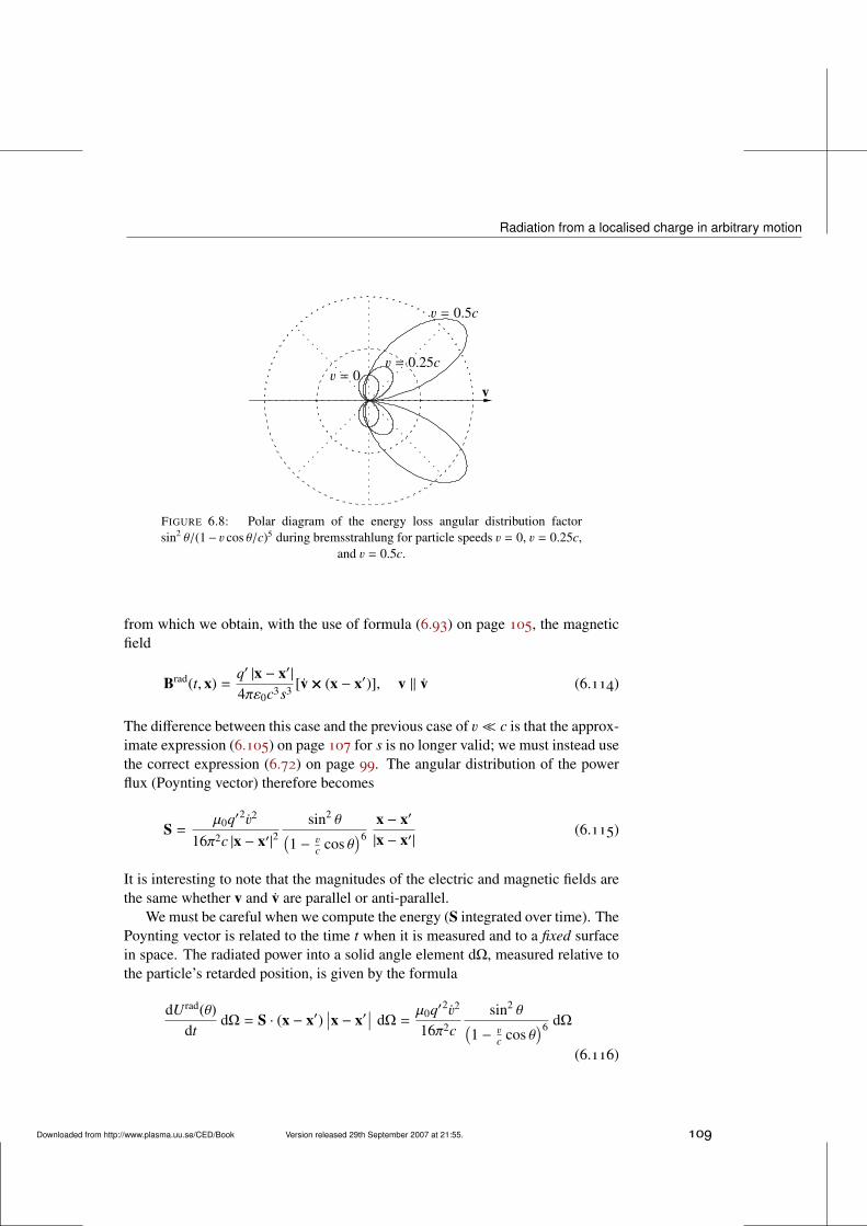
Radiation from a localised charge in arbitrary motion
v = 0v
v = 0.5c
v = 0.25c
FIGURE 6.8: Polar diagram of the energy loss angular distribution factorsin2 θ/(1− v cos θ/c)5 during bremsstrahlung for particle speeds v = 0, v = 0.25c,
and v = 0.5c.
from which we obtain, with the use of formula (6.93) on page 105, the magneticfield
Brad(t, x) =q′ |x − x′|4πε0c3s3 [v × (x − x′)], v ‖ v (6.114)
The difference between this case and the previous case of v c is that the approx-imate expression (6.105) on page 107 for s is no longer valid; we must instead usethe correct expression (6.72) on page 99. The angular distribution of the powerflux (Poynting vector) therefore becomes
S =µ0q′2v2
16π2c |x − x′|2sin2 θ(
1 − vc cos θ
)6x − x′
|x − x′|(6.115)
It is interesting to note that the magnitudes of the electric and magnetic fields arethe same whether v and v are parallel or anti-parallel.
We must be careful when we compute the energy (S integrated over time). ThePoynting vector is related to the time t when it is measured and to a fixed surfacein space. The radiated power into a solid angle element dΩ, measured relative tothe particle’s retarded position, is given by the formula
dUrad(θ)dt
dΩ = S · (x − x′)∣∣x − x′
∣∣ dΩ =µ0q′2v2
16π2csin2 θ(
1 − vc cos θ
)6 dΩ
(6.116)
Downloaded from http://www.plasma.uu.se/CED/Book Version released 29th September 2007 at 21:55. 109
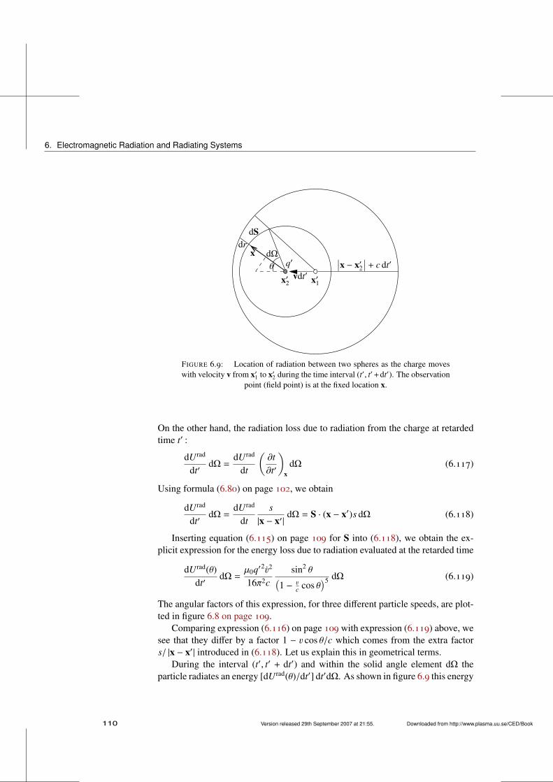
6. Electromagnetic Radiation and Radiating Systems
x′1x′2vdt′
∣∣x − x′2∣∣ + c dt′
dSdr
xθ
dΩq′
FIGURE 6.9: Location of radiation between two spheres as the charge moveswith velocity v from x′1 to x′2 during the time interval (t′, t′+dt′). The observation
point (field point) is at the fixed location x.
On the other hand, the radiation loss due to radiation from the charge at retardedtime t′ :
dUrad
dt′dΩ =
dUrad
dt
(∂t∂t′
)x
dΩ (6.117)
Using formula (6.80) on page 102, we obtain
dUrad
dt′dΩ =
dUrad
dts
|x − x′|dΩ = S · (x − x′)s dΩ (6.118)
Inserting equation (6.115) on page 109 for S into (6.118), we obtain the ex-plicit expression for the energy loss due to radiation evaluated at the retarded time
dUrad(θ)dt′
dΩ =µ0q′2v2
16π2csin2 θ(
1 − vc cos θ
)5 dΩ (6.119)
The angular factors of this expression, for three different particle speeds, are plot-ted in figure 6.8 on page 109.
Comparing expression (6.116) on page 109 with expression (6.119) above, wesee that they differ by a factor 1 − v cos θ/c which comes from the extra factors/ |x − x′| introduced in (6.118). Let us explain this in geometrical terms.
During the interval (t′, t′ + dt′) and within the solid angle element dΩ theparticle radiates an energy [dUrad(θ)/dt′] dt′dΩ. As shown in figure 6.9 this energy
110 Version released 29th September 2007 at 21:55. Downloaded from http://www.plasma.uu.se/CED/Book
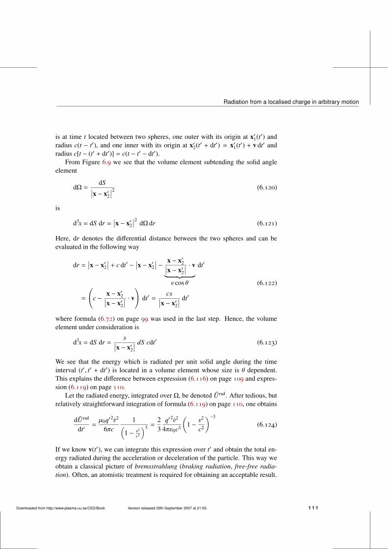
Radiation from a localised charge in arbitrary motion
is at time t located between two spheres, one outer with its origin at x′1(t′) andradius c(t − t′), and one inner with its origin at x′2(t′ + dt′) = x′1(t′) + v dt′ andradius c[t − (t′ + dt′)] = c(t − t′ − dt′).
From Figure 6.9 we see that the volume element subtending the solid angleelement
dΩ =dS∣∣x − x′2
∣∣2 (6.120)
is
d3x = dS dr =∣∣x − x′2
∣∣2 dΩ dr (6.121)
Here, dr denotes the differential distance between the two spheres and can beevaluated in the following way
dr =∣∣x − x′2
∣∣ + c dt′ −∣∣x − x′2
∣∣ − x − x′2∣∣x − x′2∣∣ · v︸ ︷︷ ︸
v cos θ
dt′
=
(c −
x − x′2∣∣x − x′2∣∣ · v
)dt′ =
cs∣∣x − x′2∣∣ dt′
(6.122)
where formula (6.72) on page 99 was used in the last step. Hence, the volumeelement under consideration is
d3x = dS dr =s∣∣x − x′2∣∣ dS cdt′ (6.123)
We see that the energy which is radiated per unit solid angle during the timeinterval (t′, t′ + dt′) is located in a volume element whose size is θ dependent.This explains the difference between expression (6.116) on page 109 and expres-sion (6.119) on page 110.
Let the radiated energy, integrated over Ω, be denoted Urad. After tedious, butrelatively straightforward integration of formula (6.119) on page 110, one obtains
dUrad
dt′=µ0q′2v2
6πc1(
1 − v2
c2
)3 =23
q′2v2
4πε0c3
(1 −
v2
c2
)−3
(6.124)
If we know v(t′), we can integrate this expression over t′ and obtain the total en-ergy radiated during the acceleration or deceleration of the particle. This way weobtain a classical picture of bremsstrahlung (braking radiation, free-free radia-tion). Often, an atomistic treatment is required for obtaining an acceptable result.
Downloaded from http://www.plasma.uu.se/CED/Book Version released 29th September 2007 at 21:55. 111
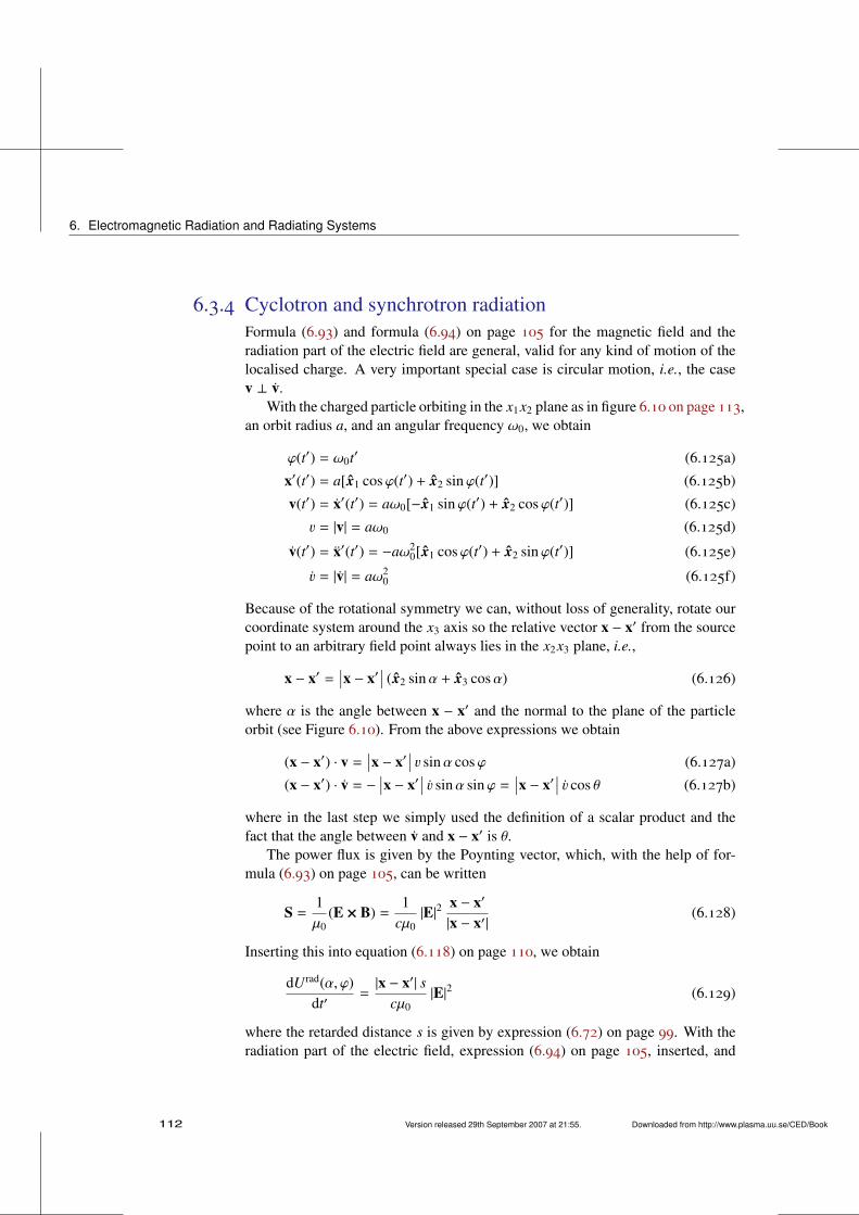
6. Electromagnetic Radiation and Radiating Systems
6.3.4 Cyclotron and synchrotron radiationFormula (6.93) and formula (6.94) on page 105 for the magnetic field and theradiation part of the electric field are general, valid for any kind of motion of thelocalised charge. A very important special case is circular motion, i.e., the casev ⊥ v.
With the charged particle orbiting in the x1x2 plane as in figure 6.10 on page 113,an orbit radius a, and an angular frequency ω0, we obtain
ϕ(t′) = ω0t′ (6.125a)
x′(t′) = a[x1 cosϕ(t′) + x2 sinϕ(t′)] (6.125b)
v(t′) = x′(t′) = aω0[−x1 sinϕ(t′) + x2 cosϕ(t′)] (6.125c)
v = |v| = aω0 (6.125d)
v(t′) = x′(t′) = −aω20[x1 cosϕ(t′) + x2 sinϕ(t′)] (6.125e)
v = |v| = aω20 (6.125f)
Because of the rotational symmetry we can, without loss of generality, rotate ourcoordinate system around the x3 axis so the relative vector x − x′ from the sourcepoint to an arbitrary field point always lies in the x2x3 plane, i.e.,
x − x′ =∣∣x − x′
∣∣ (x2 sinα + x3 cosα) (6.126)
where α is the angle between x − x′ and the normal to the plane of the particleorbit (see Figure 6.10). From the above expressions we obtain
(x − x′) · v =∣∣x − x′
∣∣ v sinα cosϕ (6.127a)
(x − x′) · v = −∣∣x − x′
∣∣ v sinα sinϕ =∣∣x − x′
∣∣ v cos θ (6.127b)
where in the last step we simply used the definition of a scalar product and thefact that the angle between v and x − x′ is θ.
The power flux is given by the Poynting vector, which, with the help of for-mula (6.93) on page 105, can be written
S =1µ0
(E × B) =1
cµ0|E|2
x − x′
|x − x′|(6.128)
Inserting this into equation (6.118) on page 110, we obtain
dUrad(α, ϕ)dt′
=|x − x′| s
cµ0|E|2 (6.129)
where the retarded distance s is given by expression (6.72) on page 99. With theradiation part of the electric field, expression (6.94) on page 105, inserted, and
112 Version released 29th September 2007 at 21:55. Downloaded from http://www.plasma.uu.se/CED/Book
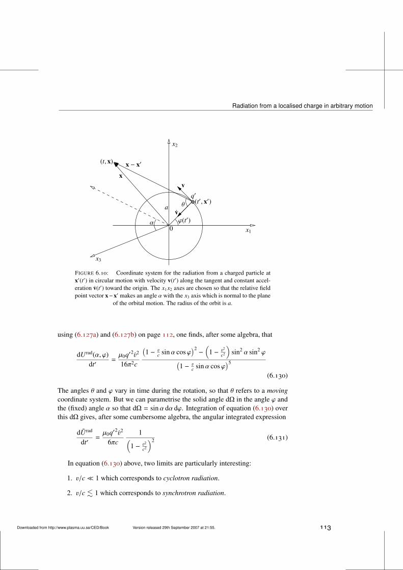
Radiation from a localised charge in arbitrary motion
v
x1
x3
x2
ϕ(t′)0
α
av
(t, x) x − x′
x
(t′, x′)θ
q′
FIGURE 6.10: Coordinate system for the radiation from a charged particle atx′(t′) in circular motion with velocity v(t′) along the tangent and constant accel-eration v(t′) toward the origin. The x1 x2 axes are chosen so that the relative fieldpoint vector x−x′ makes an angle α with the x3 axis which is normal to the plane
of the orbital motion. The radius of the orbit is a.
using (6.127a) and (6.127b) on page 112, one finds, after some algebra, that
dUrad(α, ϕ)dt′
=µ0q′2v2
16π2c
(1 − v
c sinα cosϕ)2−
(1 − v2
c2
)sin2 α sin2 ϕ(
1 − vc sinα cosϕ
)5
(6.130)
The angles θ and ϕ vary in time during the rotation, so that θ refers to a movingcoordinate system. But we can parametrise the solid angle dΩ in the angle ϕ andthe (fixed) angle α so that dΩ = sinα dα dϕ. Integration of equation (6.130) overthis dΩ gives, after some cumbersome algebra, the angular integrated expression
dUrad
dt′=µ0q′2v2
6πc1(
1 − v2
c2
)2 (6.131)
In equation (6.130) above, two limits are particularly interesting:
1. v/c 1 which corresponds to cyclotron radiation.
2. v/c . 1 which corresponds to synchrotron radiation.
Downloaded from http://www.plasma.uu.se/CED/Book Version released 29th September 2007 at 21:55. 113
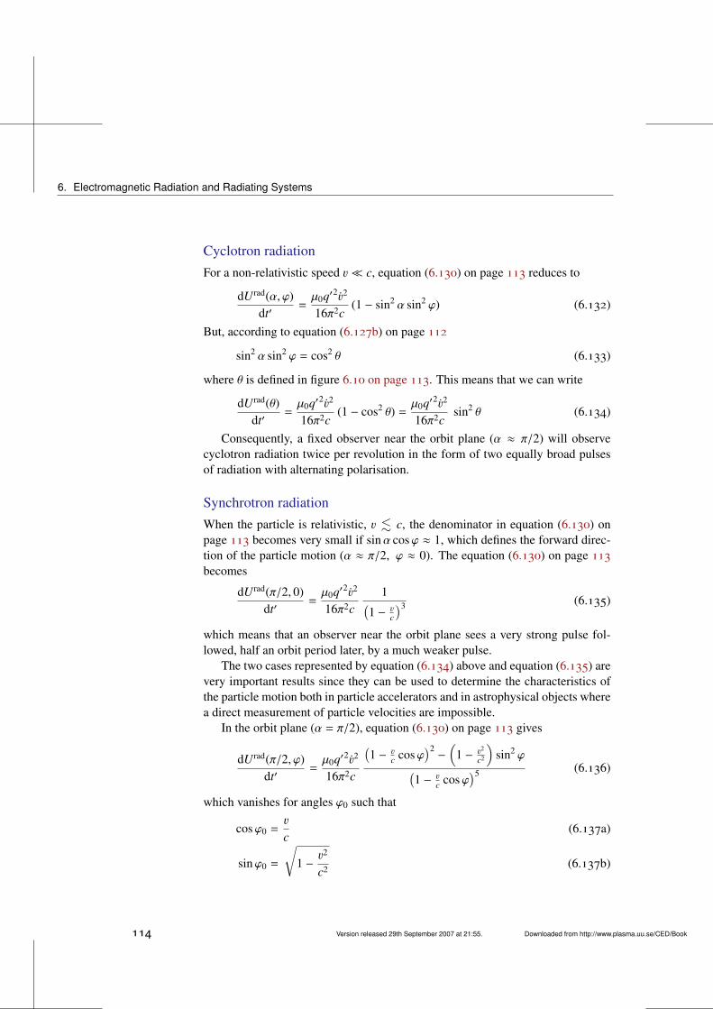
6. Electromagnetic Radiation and Radiating Systems
Cyclotron radiationFor a non-relativistic speed v c, equation (6.130) on page 113 reduces to
dUrad(α, ϕ)dt′
=µ0q′2v2
16π2c(1 − sin2 α sin2 ϕ) (6.132)
But, according to equation (6.127b) on page 112
sin2 α sin2 ϕ = cos2 θ (6.133)
where θ is defined in figure 6.10 on page 113. This means that we can write
dUrad(θ)dt′
=µ0q′2v2
16π2c(1 − cos2 θ) =
µ0q′2v2
16π2csin2 θ (6.134)
Consequently, a fixed observer near the orbit plane (α ≈ π/2) will observecyclotron radiation twice per revolution in the form of two equally broad pulsesof radiation with alternating polarisation.
Synchrotron radiationWhen the particle is relativistic, v . c, the denominator in equation (6.130) onpage 113 becomes very small if sinα cosϕ ≈ 1, which defines the forward direc-tion of the particle motion (α ≈ π/2, ϕ ≈ 0). The equation (6.130) on page 113becomes
dUrad(π/2, 0)dt′
=µ0q′2v2
16π2c1(
1 − vc
)3 (6.135)
which means that an observer near the orbit plane sees a very strong pulse fol-lowed, half an orbit period later, by a much weaker pulse.
The two cases represented by equation (6.134) above and equation (6.135) arevery important results since they can be used to determine the characteristics ofthe particle motion both in particle accelerators and in astrophysical objects wherea direct measurement of particle velocities are impossible.
In the orbit plane (α = π/2), equation (6.130) on page 113 gives
dUrad(π/2, ϕ)dt′
=µ0q′2v2
16π2c
(1 − v
c cosϕ)2−
(1 − v2
c2
)sin2 ϕ(
1 − vc cosϕ
)5 (6.136)
which vanishes for angles ϕ0 such that
cosϕ0 =v
c(6.137a)
sinϕ0 =
√1 −
v2
c2 (6.137b)
114 Version released 29th September 2007 at 21:55. Downloaded from http://www.plasma.uu.se/CED/Book
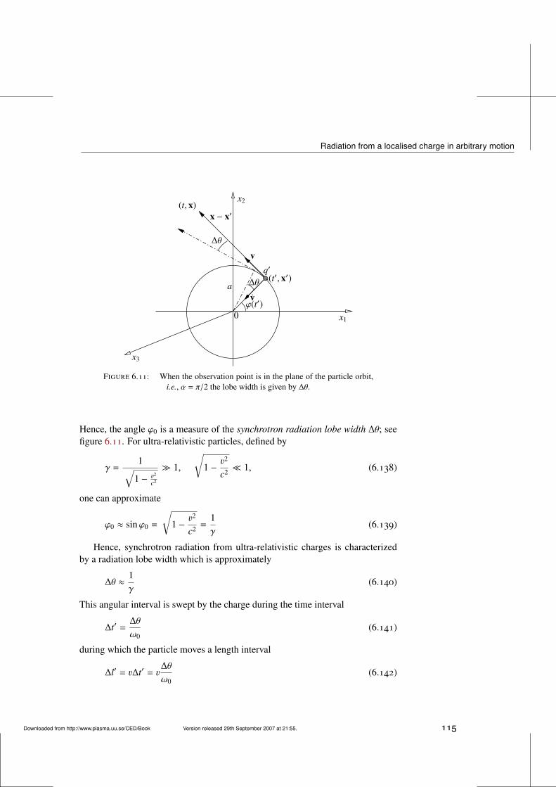
Radiation from a localised charge in arbitrary motion
v
x1
x3
x2
ϕ(t′)0
a ∆θ
∆θ
v
(t, x)x − x′
(t′, x′)q′
FIGURE 6.11: When the observation point is in the plane of the particle orbit,i.e., α = π/2 the lobe width is given by ∆θ.
Hence, the angle ϕ0 is a measure of the synchrotron radiation lobe width ∆θ; seefigure 6.11. For ultra-relativistic particles, defined by
γ =1√
1 − v2
c2
1,
√1 −
v2
c2 1, (6.138)
one can approximate
ϕ0 ≈ sinϕ0 =
√1 −
v2
c2 =1γ
(6.139)
Hence, synchrotron radiation from ultra-relativistic charges is characterizedby a radiation lobe width which is approximately
∆θ ≈1γ
(6.140)
This angular interval is swept by the charge during the time interval
∆t′ =∆θ
ω0(6.141)
during which the particle moves a length interval
∆l′ = v∆t′ = v∆θ
ω0(6.142)
Downloaded from http://www.plasma.uu.se/CED/Book Version released 29th September 2007 at 21:55. 115
6. Electromagnetic Radiation and Radiating Systems
in the direction toward the observer who therefore measures a compressed pulsewidth of length
∆t = ∆t′ −∆l′
c= ∆t′ −
v∆t′
c=(
1 −v
c
)∆t′ =
(1 −
v
c
) ∆θω0≈
(1 −
v
c
) 1γω0
=
(1 − v
c
) (1 + v
c
)1 +
v
c︸ ︷︷ ︸≈ 2
1γω0
≈
(1 −
v2
c2
)︸ ︷︷ ︸
1/γ2
12γω0
=1
2γ3
1ω0
(6.143)
Typically, the spectral width of a pulse of length ∆t is ∆ω . 1/∆t. In the ultra-relativistic synchrotron case one can therefore expect frequency components upto
ωmax ≈1∆t= 2γ3ω0 (6.144)
A spectral analysis of the radiation pulse will therefore exhibit a (broadened) linespectrum of Fourier components nω0 from n = 1 up to n ≈ 2γ3.
When many charged particles, N say, contribute to the radiation, we can havethree different situations depending on the relative phases of the radiation fieldsfrom the individual particles:
1. All N radiating particles are spatially much closer to each other than a typ-ical wavelength. Then the relative phase differences of the individual elec-tric and magnetic fields radiated are negligible and the total radiated fieldsfrom all individual particles will add up to become N times that from oneparticle. This means that the power radiated from the N particles will be N2
higher than for a single charged particle. This is called coherent radiation.
2. The charged particles are perfectly evenly distributed in the orbit. In thiscase the phases of the radiation fields cause a complete cancellation of thefields themselves. No radiation escapes.
3. The charged particles are somewhat unevenly distributed in the orbit. Thishappens for an open ring current, carried initially by evenly distributedcharged particles, which is subject to thermal fluctuations. From statisti-cal mechanics we know that this happens for all open systems and that theparticle densities exhibit fluctuations of order
√N. This means that out of
the N particles,√
N will exhibit deviation from perfect randomness—andthereby perfect radiation field cancellation—and give rise to net radiationfields which are proportional to
√N. As a result, the radiated power will be
proportional to N, and we speak about incoherent radiation. Examples ofthis can be found both in earthly laboratories and under cosmic conditions.
116 Version released 29th September 2007 at 21:55. Downloaded from http://www.plasma.uu.se/CED/Book
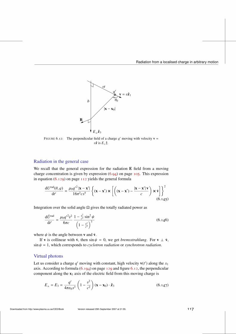
Radiation from a localised charge in arbitrary motion
θ0
vt
b
B
v = vx1q′
|x − x0|
E⊥ x3
FIGURE 6.12: The perpendicular field of a charge q′ moving with velocity v =vx is E⊥ z.
Radiation in the general caseWe recall that the general expression for the radiation E field from a movingcharge concentration is given by expression (6.94) on page 105. This expressionin equation (6.129) on page 112 yields the general formula
dUrad(θ, ϕ)dt′
=µ0q′2 |x − x′|
16π2cs5
(x − x′) ×
[((x − x′) −
|x − x′| vc
)× v]2
(6.145)
Integration over the solid angle Ω gives the totally radiated power as
dUrad
dt′=µ0q′2v2
6πc1 − v2
c2 sin2 ψ(1 − v2
c2
)3 (6.146)
where ψ is the angle between v and v.If v is collinear with v, then sinψ = 0, we get bremsstrahlung. For v ⊥ v,
sinψ = 1, which corresponds to cyclotron radiation or synchrotron radiation.
Virtual photonsLet us consider a charge q′ moving with constant, high velocity v(t′) along the x1
axis. According to formula (6.194) on page 129 and figure 6.12, the perpendicularcomponent along the x3 axis of the electric field from this moving charge is
E⊥ = E3 =q′
4πε0s3
(1 −
v2
c2
)(x − x0) · x3 (6.147)
Downloaded from http://www.plasma.uu.se/CED/Book Version released 29th September 2007 at 21:55. 117
6. Electromagnetic Radiation and Radiating Systems
Utilising expression (6.103) on page 107 and simple geometrical relations, we canrewrite this as
E⊥ =q′
4πε0
b
γ2[(vt)2 + b2/γ2
]3/2 (6.148)
This represents a contracted Coulomb field, approaching the field of a plane wave.The passage of this field ‘pulse’ corresponds to a frequency distribution of the fieldenergy. Fourier transforming, we obtain
Eω,⊥ =1
2π
∫ ∞−∞
dt E⊥(t) eiωt =q′
4π2ε0bv
[(bωvγ
)K1
(bωvγ
)](6.149)
Here, K1 is the Kelvin function (Bessel function of the second kind with imaginaryargument) which behaves in such a way for small and large arguments that
Eω,⊥ ∼q′
4π2ε0bv, bω vγ ⇔
bvγω 1 (6.150a)
Eω,⊥ ∼ 0, bω vγ ⇔bvγω 1 (6.150b)
showing that the ‘pulse’ length is of the order b/(vγ).Due to the equipartitioning of the field energy into the electric and magnetic
fields, the total field energy can be written
U = ε0
∫V
d3x E2⊥ = ε0
∫ bmax
bmin
db 2πb∫ ∞−∞
dt vE2⊥ (6.151)
where the volume integration is over the plane perpendicular to v. With the useof Parseval’s identity for Fourier transforms, formula (5.34) on page 79, we canrewrite this as
U =∫ ∞
0dω Uω = 4πε0v
∫ bmax
bmin
db 2πb∫ ∞
0dω Eω,⊥
≈q′2
2π2ε0v
∫ ∞−∞
dω∫ vγ/ω
bmin
dbb
(6.152)
from which we conclude that
Uω ≈q′2
2π2ε0vln(
vγ
bminω
)(6.153)
where an explicit value of bmin can be calculated in quantum theory only.As in the case of bremsstrahlung, it is intriguing to quantise the energy into
photons [cf. equation (6.224) on page 133]. Then we find that
Nω dω ≈2απ
ln(
cγbminω
)dωω
(6.154)
118 Version released 29th September 2007 at 21:55. Downloaded from http://www.plasma.uu.se/CED/Book
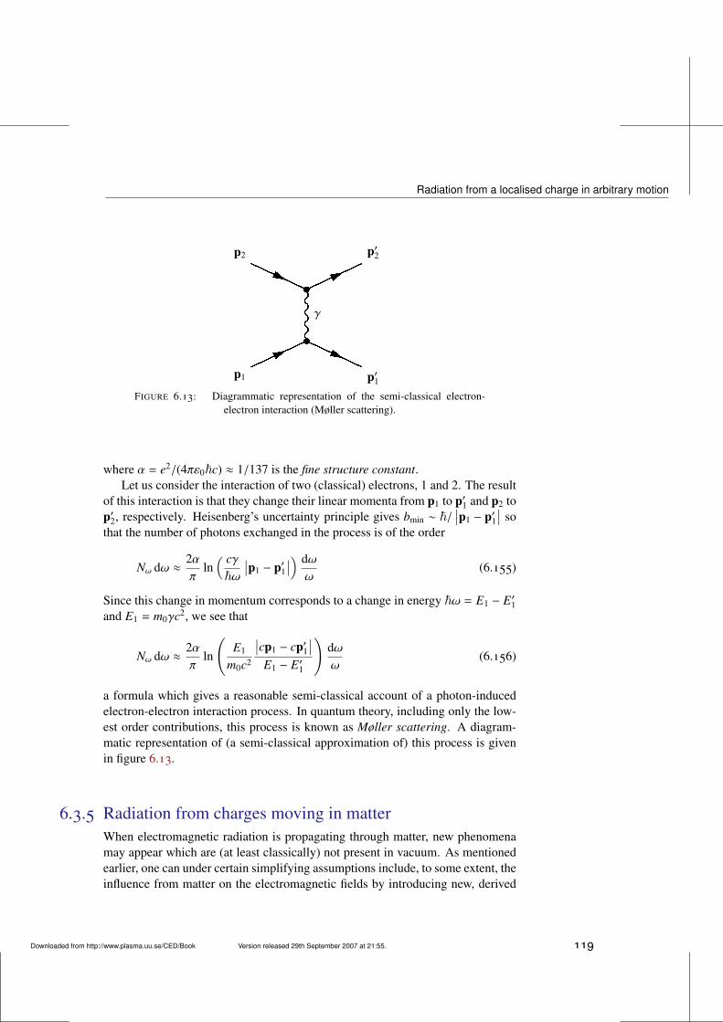
Radiation from a localised charge in arbitrary motion
γ
p1
p2
p′1
p′2
FIGURE 6.13: Diagrammatic representation of the semi-classical electron-electron interaction (Møller scattering).
where α = e2/(4πε0~c) ≈ 1/137 is the fine structure constant.Let us consider the interaction of two (classical) electrons, 1 and 2. The result
of this interaction is that they change their linear momenta from p1 to p′1 and p2 top′2, respectively. Heisenberg’s uncertainty principle gives bmin ∼ ~/
∣∣p1 − p′1∣∣ so
that the number of photons exchanged in the process is of the order
Nω dω ≈2απ
ln( cγ
~ω∣∣p1 − p′1
∣∣) dωω
(6.155)
Since this change in momentum corresponds to a change in energy ~ω = E1 − E′1and E1 = m0γc2, we see that
Nω dω ≈2απ
ln
(E1
m0c2
∣∣cp1 − cp′1∣∣
E1 − E′1
)dωω
(6.156)
a formula which gives a reasonable semi-classical account of a photon-inducedelectron-electron interaction process. In quantum theory, including only the low-est order contributions, this process is known as Møller scattering. A diagram-matic representation of (a semi-classical approximation of) this process is givenin figure 6.13.
6.3.5 Radiation from charges moving in matterWhen electromagnetic radiation is propagating through matter, new phenomenamay appear which are (at least classically) not present in vacuum. As mentionedearlier, one can under certain simplifying assumptions include, to some extent, theinfluence from matter on the electromagnetic fields by introducing new, derived
Downloaded from http://www.plasma.uu.se/CED/Book Version released 29th September 2007 at 21:55. 119
6. Electromagnetic Radiation and Radiating Systems
field quantities D and H according to
D = ε(t, x)E = κeε0E (6.157)
B = µ(t, x)H = κmµ0H (6.158)
Expressed in terms of these derived field quantities, the Maxwell equations, oftencalled macroscopic Maxwell equations, take the form
∇ · D = ρ(t, x) (6.159a)
∇ × E = −∂B∂t
(6.159b)
∇ · B = 0 (6.159c)
∇ ×H =∂D∂t+ j(t, x) (6.159d)
Assuming for simplicity that the electric permittivity ε and the magnetic per-meability µ, and hence the relative permittivity κe and the relative permeability κm
all have fixed values, independent on time and space, for each type of material weconsider, we can derive the general telegrapher’s equation [cf. equation (2.34) onpage 33]
∂2E∂ζ2 − σµ
∂E∂t− εµ
∂2E∂t2 = 0 (6.160)
describing (1D) wave propagation in a material medium.In chapter 2 we concluded that the existence of a finite conductivity, manifest-
ing itself in a collisional interaction between the charge carriers, causes the wavesto decay exponentially with time and space. Let us therefore assume that in ourmedium σ = 0 so that the wave equation simplifies to
∂2E∂ζ2 − εµ
∂2E∂t2 = 0 (6.161)
If we introduce the phase velocity in the medium as
vϕ =1√εµ=
1√κeε0κmµ0
=c√κeκm
(6.162)
where, according to equation (1.11) on page 6, c = 1/√ε0µ0 is the speed of
light, i.e., the phase speed of electromagnetic waves in vacuum, then the generalsolution to each component of equation (6.161) above
Ei = f (ζ − vϕt) + g(ζ + vϕt), i = 1, 2, 3 (6.163)
120 Version released 29th September 2007 at 21:55. Downloaded from http://www.plasma.uu.se/CED/Book
Radiation from a localised charge in arbitrary motion
The ratio of the phase speed in vacuum and in the medium
cvϕ=√κeκm = c
√εµ
def≡ n (6.164)
is called the refractive index of the medium. In general n is a function of bothtime and space as are the quantities ε, µ, κe, and κm themselves. If, in addition,the medium is anisotropic or birefringent, all these quantities are rank-two tensorfields. Under our simplifying assumptions, in each medium we consider n =Const for each frequency component of the fields.
Associated with the phase speed of a medium for a wave of a given frequencyω we have a wave vector, defined as
kdef≡ k k = kvϕ =
ω
vϕ
vϕvϕ
(6.165)
As in the vacuum case discussed in chapter 2, assuming that E is time-harmonic,i.e., can be represented by a Fourier component proportional to exp−iωt, thesolution of equation (6.161) can be written
E = E0ei(k·x−ωt) (6.166)
where now k is the wave vector in the medium given by equation (6.165). Withthese definitions, the vacuum formula for the associated magnetic field, equa-tion (2.41) on page 33,
B =√εµ k × E =
1vϕ
k × E =1ω
k × E (6.167)
is valid also in a material medium (assuming, as mentioned, that n has a fixedconstant scalar value). A consequence of a κe , 1 is that the electric field will, ingeneral, have a longitudinal component.
It is important to notice that depending on the electric and magnetic propertiesof a medium, and, hence, on the value of the refractive index n, the phase speedin the medium can be smaller or larger than the speed of light:
vϕ =cn=ω
k(6.168)
where, in the last step, we used equation (6.165).If the medium has a refractive index which, as is usually the case, dependent
on frequency ω, we say that the medium is dispersive. Because in this case alsok(ω) and ω(k), so that the group velocity
vg =∂ω
∂k(6.169)
Downloaded from http://www.plasma.uu.se/CED/Book Version released 29th September 2007 at 21:55. 121
6. Electromagnetic Radiation and Radiating Systems
has a unique value for each frequency component, and is different from vϕ. Exceptin regions of anomalous dispersion, vg is always smaller than c. In a gas of freecharges, such as a plasma, the refractive index is given by the expression
n2(ω) = 1 −ω2
p
ω2 (6.170)
where
ω2p =∑
σ
Nσq2σ
ε0mσ(6.171)
is the square of the plasma frequency ωp. Here mσ and Nσ denote the mass andnumber density, respectively, of charged particle species σ. In an inhomogeneousplasma, Nσ = Nσ(x) so that the refractive index and also the phase and groupvelocities are space dependent. As can be easily seen, for each given frequency,the phase and group velocities in a plasma are different from each other. If thefrequency ω is such that it coincides with ωp at some point in the medium, then atthat point vϕ → ∞ while vg → 0 and the wave Fourier component at ω is reflectedthere.
Vavilov-Cerenkov radiationAs we saw in subsection 6.1, a charge in uniform, rectilinear motion in vacuumdoes not give rise to any radiation; see in particular equation (6.192a) on page 128.Let us now consider a charge in uniform, rectilinear motion in a medium with elec-tric properties which are different from those of a (classical) vacuum. Specifically,consider a medium where
ε = Const > ε0 (6.172a)
µ = µ0 (6.172b)
This implies that in this medium the phase speed is
vϕ =cn=
1√εµ0
< c (6.173)
Hence, in this particular medium, the speed of propagation of (the phase planes of)electromagnetic waves is less than the speed of light in vacuum, which we knowis an absolute limit for the motion of anything, including particles. A mediumof this kind has the interesting property that particles, entering into the mediumat high speeds |v|, which, of course, are below the phase speed in vacuum, canexperience that the particle speeds are higher than the phase speed in the medium.This is the basis for the Vavilov-Cerenkov radiation, more commonly known asCerenkov radiation, that we shall now study.
122 Version released 29th September 2007 at 21:55. Downloaded from http://www.plasma.uu.se/CED/Book
Radiation from a localised charge in arbitrary motion
If we recall the general derivation, in the vacuum case, of the retarded (and ad-vanced) potentials in chapter 3 and the Liénard-Wiechert potentials, equations (6.71)on page 99, we realise that we obtain the latter in the medium by a simple for-mal replacement c → c/n in the expression (6.72) on page 99 for s. Hence, theLiénard-Wiechert potentials in a medium characterized by a refractive index n,are
φ(t, x) =1
4πε0
q′∣∣|x − x′| − n (x−x′)·vc
∣∣ = 14πε0
q′
s(6.174a)
A(t, x) =1
4πε0c2
q′v∣∣|x − x′| − n (x−x′)·vc
∣∣ = 14πε0c2
q′vs
(6.174b)
where now
s =∣∣∣∣∣∣x − x′
∣∣ − n(x − x′) · v
c
∣∣∣∣ (6.175)
The need for the absolute value of the expression for s is obvious in the casewhen v/c ≥ 1/n because then the second term can be larger than the first term;if v/c 1/n we recover the well-known vacuum case but with modified phasespeed. We also note that the retarded and advanced times in the medium are [cf.equation (3.32) on page 50]
t′ret = t′ret(t,∣∣x − x′
∣∣) = t −k |x − x′|
ω= t −
|x − x′| nc
(6.176a)
t′adv = t′adv(t,∣∣x − x′
∣∣) = t +k |x − x′|
ω= t +
|x − x′| nc
(6.176b)
so that the usual time interval t − t′ between the time measured at the point ofobservation and the retarded time in a medium becomes
t − t′ =|x − x′| n
c(6.177)
For v/c ≥ 1/n, the retarded distance s, and therefore the denominators inequations (6.174) above, vanish when
n(x − x′) ·vc=∣∣x − x′
∣∣ nvc
cos θc =∣∣x − x′
∣∣ (6.178)
or, equivalently, when
cos θc =cnv
(6.179)
In the direction defined by this angle θc, the potentials become singular. Duringthe time interval t − t′ given by expression (6.177), the field exists within a sphereof radius |x − x′| around the particle while the particle moves a distance
l′ = (t − t′)v (6.180)
Downloaded from http://www.plasma.uu.se/CED/Book Version released 29th September 2007 at 21:55. 123
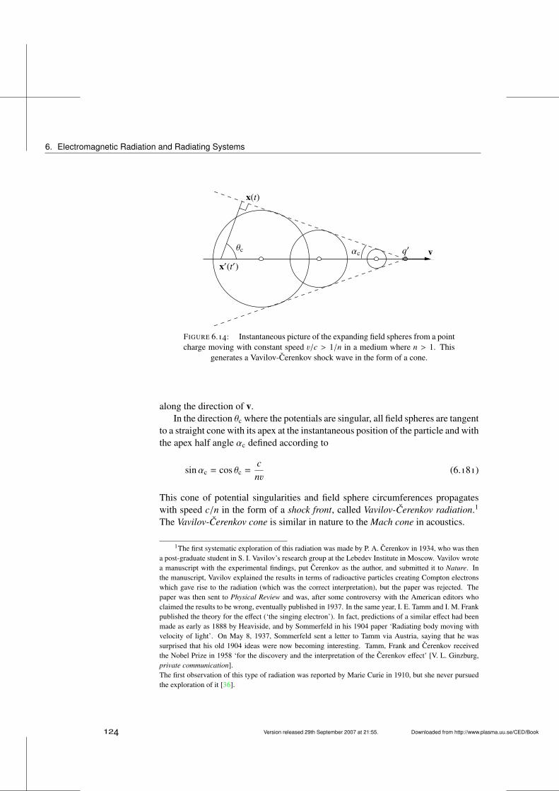
6. Electromagnetic Radiation and Radiating Systems
θc αc vq′
x′(t′)
x(t)
FIGURE 6.14: Instantaneous picture of the expanding field spheres from a pointcharge moving with constant speed v/c > 1/n in a medium where n > 1. This
generates a Vavilov-Cerenkov shock wave in the form of a cone.
along the direction of v.In the direction θc where the potentials are singular, all field spheres are tangent
to a straight cone with its apex at the instantaneous position of the particle and withthe apex half angle αc defined according to
sinαc = cos θc =cnv
(6.181)
This cone of potential singularities and field sphere circumferences propagateswith speed c/n in the form of a shock front, called Vavilov-Cerenkov radiation.1
The Vavilov-Cerenkov cone is similar in nature to the Mach cone in acoustics.
1The first systematic exploration of this radiation was made by P. A. Cerenkov in 1934, who was thena post-graduate student in S. I. Vavilov’s research group at the Lebedev Institute in Moscow. Vavilov wrotea manuscript with the experimental findings, put Cerenkov as the author, and submitted it to Nature. Inthe manuscript, Vavilov explained the results in terms of radioactive particles creating Compton electronswhich gave rise to the radiation (which was the correct interpretation), but the paper was rejected. Thepaper was then sent to Physical Review and was, after some controversy with the American editors whoclaimed the results to be wrong, eventually published in 1937. In the same year, I. E. Tamm and I. M. Frankpublished the theory for the effect (‘the singing electron’). In fact, predictions of a similar effect had beenmade as early as 1888 by Heaviside, and by Sommerfeld in his 1904 paper ‘Radiating body moving withvelocity of light’. On May 8, 1937, Sommerfeld sent a letter to Tamm via Austria, saying that he wassurprised that his old 1904 ideas were now becoming interesting. Tamm, Frank and Cerenkov receivedthe Nobel Prize in 1958 ‘for the discovery and the interpretation of the Cerenkov effect’ [V. L. Ginzburg,private communication].The first observation of this type of radiation was reported by Marie Curie in 1910, but she never pursuedthe exploration of it [36].
124 Version released 29th September 2007 at 21:55. Downloaded from http://www.plasma.uu.se/CED/Book
Radiation from a localised charge in arbitrary motion
In order to make some quantitative estimates of this radiation, we note that wecan describe the motion of each charged particle q′ as a current density:
j = q′v δ(x′ − vt′) = q′v δ(x′ − vt′)δ(y′)δ(z′)x1 (6.182)
which has the trivial Fourier transform
jω =q′
2πeiωx′/v δ(y′)δ(z′)x1 (6.183)
This Fourier component can be used in the formulae derived for a linear currentin subsection 6.1.1 if only we make the replacements
ε0 → ε = n2ε0 (6.184a)
k →nωc
(6.184b)
In this manner, using jω from equation (6.183) above, the resulting Fourier trans-forms of the Vavilov-Cerenkov magnetic and electric radiation fields can be calcu-lated from the expressions (5.10) on page 72) and (5.21) on page 74, respectively.
The total energy content is then obtained from equation (5.34) on page 79(integrated over a closed sphere at large distances). For a Fourier component oneobtains [cf. equation (5.37) on page 80]
Uradω dΩ ≈
14πε0nc
∣∣∣∣∫V ′
d3x′ (jω × k)e−ik·x′∣∣∣∣2 dΩ
=q′2nω2
16π3ε0c3
∣∣∣∣∫ ∞−∞
exp[ix′(ωv− k cos θ
)]dx′∣∣∣∣2 sin2 θ dΩ
(6.185)
where θ is the angle between the direction of motion, x′1, and the direction to theobserver, k. The integral in (6.185) is singular of a ‘Dirac delta type’. If we limitthe spatial extent of the motion of the particle to the closed interval [−X, X] on thex′ axis we can evaluate the integral to obtain
Uradω dΩ =
q′2nω2 sin2 θ
4π3ε0c3
sin2 [(1 − nvc cos θ
)Xωv
][(1 − nv
c cos θ)ωv
]2 dΩ (6.186)
which has a maximum in the direction θc as expected. The magnitude of thismaximum grows and its width narrows as X → ∞. The integration of (6.186)over Ω therefore picks up the main contributions from θ ≈ θc. Consequently, wecan set sin2 θ ≈ sin2 θc and the result of the integration is
Uradω = 2π
∫ π
0Uradω (θ) sin θ dθ = dcos θ = −ξc = 2π
∫ 1
−1Uradω (ξ) dξ
≈q′2nω2 sin2 θc
2π2ε0c3
∫ 1
−1
sin2 [(1 + nvξc
)Xωv
][(1 + nvξ
c
)ωv
]2 dξ(6.187)
Downloaded from http://www.plasma.uu.se/CED/Book Version released 29th September 2007 at 21:55. 125
6. Electromagnetic Radiation and Radiating Systems
The integrand in (6.187) is strongly peaked near ξ = −c/(nv), or, equivalently,near cos θc = c/(nv). This means that the integrand function is practically zerooutside the integration interval ξ ∈ [−1, 1]. Consequently, one may extend theξ integration interval to (−∞,∞) without introducing too much an error. Via yetanother variable substitution we can therefore approximate
sin2 θc
∫ 1
−1
sin2 [(1 + nvξc
)Xωv
][(1 + nvξ
c
)ωv
]2 dξ ≈(
1 −c2
n2v2
)cXωn
∫ ∞−∞
sin2 xx2 dx
=cXπωn
(1 −
c2
n2v2
) (6.188)
leading to the final approximate result for the total energy loss in the frequencyinterval (ω,ω + dω)
Uradω dω =
q′2X2πε0c2
(1 −
c2
n2v2
)ω dω (6.189)
As mentioned earlier, the refractive index is usually frequency dependent. Re-alising this, we find that the radiation energy per frequency unit and per unit lengthis
Uradω dω2X
=q′2ω
4πε0c2
(1 −
c2
n2(ω)v2
)dω (6.190)
This result was derived under the assumption that v/c > 1/n(ω), i.e., under thecondition that the expression inside the parentheses in the right hand side is pos-itive. For all media it is true that n(ω) → 1 when ω → ∞, so there exist alwaysa highest frequency for which we can obtain Vavilov-Cerenkov radiation from afast charge in a medium. Our derivation above for a fixed value of n is valid foreach individual Fourier component.
6.4 Bibliography[1] H. ALFVÉN AND N. HERLOFSON, Cosmic radiation and radio stars, Physical Review, 78
(1950), p. 616.
[2] R. BECKER, Electromagnetic Fields and Interactions, Dover Publications, Inc.,New York, NY, 1982, ISBN 0-486-64290-9.
[3] M. BORN AND E. WOLF, Principles of Optics. Electromagnetic Theory of Propaga-tion, Interference and Diffraction of Light, sixth ed., Pergamon Press, Oxford,. . . , 1980,ISBN 0-08-026481-6.
126 Version released 29th September 2007 at 21:55. Downloaded from http://www.plasma.uu.se/CED/Book
Bibliography
[4] V. L. GINZBURG, Applications of Electrodynamics in Theoretical Physics and Astro-physics, Revised third ed., Gordon and Breach Science Publishers, New York, London,Paris, Montreux, Tokyo and Melbourne, 1989, ISBN 2-88124-719-9.
[5] J. D. JACKSON, Classical Electrodynamics, third ed., John Wiley & Sons, Inc.,New York, NY . . . , 1999, ISBN 0-471-30932-X.
[6] J. B. MARION AND M. A. HEALD, Classical Electromagnetic Radiation, second ed.,Academic Press, Inc. (London) Ltd., Orlando, . . . , 1980, ISBN 0-12-472257-1.
[7] W. K. H. PANOFSKY AND M. PHILLIPS, Classical Electricity and Magnetism, second ed.,Addison-Wesley Publishing Company, Inc., Reading, MA . . . , 1962, ISBN 0-201-05702-6.
[8] J. SCHWINGER, L. L. DERAAD, JR., K. A. MILTON, AND W. TSAI, Classical Electrody-namics, Perseus Books, Reading, MA, 1998, ISBN 0-7382-0056-5.
[9] J. A. STRATTON, Electromagnetic Theory, McGraw-Hill Book Company, Inc., NewYork, NY and London, 1953, ISBN 07-062150-0.
[10] J. VANDERLINDE, Classical Electromagnetic Theory, John Wiley & Sons, Inc., NewYork, Chichester, Brisbane, Toronto, and Singapore, 1993, ISBN 0-471-57269-1.
Downloaded from http://www.plasma.uu.se/CED/Book Version released 29th September 2007 at 21:55. 127
6. Electromagnetic Radiation and Radiating Systems
6.5 Examples
BTHE FIELDS FROM A UNIFORMLY MOVING CHARGEEXAMPLE 6.1
In the special case of uniform motion, the localised charge moves in a field-free, isolatedspace and we know that it will not be affected by any external forces. It will therefore moveuniformly in a straight line with the constant velocity v. This gives us the possibility to extrapo-late its position at the observation time, x′(t), from its position at the retarded time, x′(t′). Sincethe particle is not accelerated, v ≡ 0, the virtual simultaneous coordinate x0 will be identical tothe actual simultaneous coordinate of the particle at time t, i.e., x0(t) = x′(t). As depicted infigure 6.7 on page 100, the angle between x − x0 and v is θ0 while then angle between x − x′and v is θ′.
We note that in the case of uniform velocity v, time and space derivatives are closely relatedin the following way when they operate on functions of x(t) [cf. equation (1.33) on page 13]:
∂
∂t→ −v · ∇ (6.191)
Hence, the E and B fields can be obtained from formulae (6.73) on page 100, with the potentialsgiven by equations (6.71) on page 99 as follows:
E = −∇φ −∂A∂t= −∇φ −
1c2
∂vφ∂t= −∇φ −
vc2
∂φ
∂t
= −∇φ +vc
(vc· ∇φ
)= −
(1 −
vvc2 ·
)∇φ
=(vv
c2 − 1)· ∇φ
(6.192a)
B = ∇ × A = ∇ ×( v
c2 φ)= ∇φ ×
vc2 = −
vc2 × ∇φ
=vc2 ×
[(vc· ∇φ
) vc− ∇φ
]=
vc2 ×
(vvc2 − 1
)· ∇φ
=vc2 × E
(6.192b)
Here 1 = xi xi is the unit dyad and we used the fact that v × v ≡ 0. What remains is just toexpress ∇φ in quantities evaluated at t and x.
From equation (6.71a) on page 99 and equation (6.104) on page 107 we find that
∇φ =q′
4πε0∇
(1s
)= −
q′
8πε0 s3 ∇s2
= −q′
4πε0 s3
[(x − x0) +
vc×
(vc× (x − x0)
)] (6.193)
When this expression for ∇φ is inserted into equation (6.192a), the following result
128 Version released 29th September 2007 at 21:55. Downloaded from http://www.plasma.uu.se/CED/Book
Examples
E(t, x) =(vv
c2 − 1)· ∇φ = −
q′
8πε0 s3
(vvc2 − 1
)· ∇s2
=q′
4πε0 s3
(x − x0) +
vc×
(vc× (x − x0)
)−
vc
(vc· (x − x0)
)−
vvc2 ·
[vc×
(vc× (x − x0)
)]=
q′
4πε0 s3
[(x − x0) +
vc
(vc· (x − x0)
)− (x − x0)
v2
c2
−vc
(vc· (x − x0)
)]=
q′
4πε0 s3 (x − x0)(
1 −v2
c2
)
(6.194)
follows. Of course, the same result also follows from equation (6.90) on page 104 with v ≡ 0inserted.
From equation (6.194) we conclude that E is directed along the vector from the simultane-ous coordinate x0(t) to the field (observation) coordinate x(t). In a similar way, the magneticfield can be calculated and one finds that
B(t, x) =µ0q′
4πs3
(1 −
v2
c2
)v × (x − x0) =
1c2 v × E (6.195)
From these explicit formulae for the E and B fields and formula (6.103b) on page 107 for s, wecan discern the following cases:
1. v→ 0⇒ E goes over into the Coulomb field ECoulomb
2. v→ 0⇒ B goes over into the Biot-Savart field
3. v→ c⇒ E becomes dependent on θ0
4. v→ c, sin θ0 ≈ 0⇒ E→ (1 − v2/c2)ECoulomb
5. v→ c, sin θ0 ≈ 1⇒ E→ (1 − v2/c2)−1/2ECoulomb
C END OF EXAMPLE 6.1
BTHE CONVECTION POTENTIAL AND THE CONVECTION FORCE EXAMPLE 6.2
Let us consider in more detail the treatment of the radiation from a uniformly moving rigidcharge distribution.
If we return to the original definition of the potentials and the inhomogeneous wave equa-tion, formula (3.17) on page 47, for a generic potential component Ψ(t, x) and a generic sourcecomponent f (t, x),
2Ψ(t, x) =(
1c2
∂2
∂t2 − ∇2
)Ψ(t, x) = f (t, x) (6.196)
Downloaded from http://www.plasma.uu.se/CED/Book Version released 29th September 2007 at 21:55. 129
6. Electromagnetic Radiation and Radiating Systems
we find that under the assumption that v = vx1, this equation can be written(1 −
v2
c2
)∂2Ψ
∂x21+∂2Ψ
∂x22+∂2Ψ
∂x23= − f (x) (6.197)
i.e., in a time-independent form. Transforming
ξ1 =x1
√1 − v2/c2
(6.198a)
ξ2 = x2 (6.198b)
ξ3 = x3 (6.198c)
and introducing the vectorial nabla operator in ξ space, ∇ξ ≡def (∂/∂ξ1, ∂/∂ξ2, ∂/∂ξ3), the time-independent equation (6.197) reduces to an ordinary Poisson equation
∇2ξΨ(ξ) = − f (
√1 − v2/c2 ξ1, ξ2, ξ3) ≡ − f (ξ) (6.199)
in this space. This equation has the well-known Coulomb potential solution
Ψ(ξ) =1
4π
∫V
f (ξ′)|ξ − ξ′|
d3ξ′ (6.200)
After inverse transformation back to the original coordinates, this becomes
Ψ(x) =1
4π
∫V
f (x′)s
d3x′ (6.201)
where, in the denominator,
s =[
(x1 − x′1)2 +
(1 −
v2
c2
)[(x2 − x′2)2 + (x3 − x′3)2]
] 12
(6.202)
Applying this to the explicit scalar and vector potential components, realising that for a rigidcharge distribution ρ moving with velocity v the current is given by j = ρv, we obtain
φ(t, x) =1
4πε0
∫V
ρ(x′)s
d3x′ (6.203a)
A(t, x) =1
4πε0c2
∫V
vρ(x′)s
d3x′ =vc2 φ(t, x) (6.203b)
For a localised charge where∫ρ d3x′ = q′, these expressions reduce to
φ(t, x) =q′
4πε0 s(6.204a)
A(t, x) =q′v
4πε0c2 s(6.204b)
which we recognise as the Liénard-Wiechert potentials; cf. equations (6.71) on page 99. Wenotice, however, that the derivation here, based on a mathematical technique which in fact is aLorentz transformation, is of more general validity than the one leading to equations (6.71) onpage 99.
Let us now consider the action of the fields produced from a moving, rigid charge distri-bution represented by q′ moving with velocity v, on a charged particle q, also moving withvelocity v. This force is given by the Lorentz force
130 Version released 29th September 2007 at 21:55. Downloaded from http://www.plasma.uu.se/CED/Book
Examples
F = q(E + v × B) (6.205)
With the help of equation (6.195) on page 129 and equations (6.203) on page 130, and thefact that ∂t = −v · ∇ [cf. formula (6.191) on page 128], we can rewrite expression (6.205) as
F = q[E + v ×
( vc2 × E
)]= q[(v
c· ∇φ
) vc− ∇φ −
vc×
(vc× ∇φ
)](6.206)
Applying the ‘bac-cab’ rule, formula (F.51) on page 180, on the last term yields
vc×
(vc× ∇φ
)=(v
c· ∇φ
) vc−v2
c2∇φ (6.207)
which means that we can write
F = −q∇ψ (6.208)
where
ψ =
(1 −
v2
c2
)φ (6.209)
The scalar function ψ is called the convection potential or the Heaviside potential. When therigid charge distribution is well localised so that we can use the potentials (6.204) the convectionpotential becomes
ψ =
(1 −
v2
c2
)q′
4πε0 s(6.210)
The convection potential from a point charge is constant on flattened ellipsoids of revolution,defined through equation (6.202) on page 130 as(
x1 − x′1√
1 − v2/c2
)2
+ (x2 − x′2)2 + (x3 − x′3)2
= γ2(x1 − x′1)2 + (x2 − x′2)2 + (x3 − x′3)2 = Const
(6.211)
These Heaviside ellipsoids are equipotential surfaces, and since the force is proportional to thegradient of ψ, which means that it is perpendicular to the ellipsoid surface, the force betweentwo charges is in general not directed along the line which connects the charges. A consequenceof this is that a system consisting of two co-moving charges connected with a rigid bar, willexperience a torque. This is the idea behind the Trouton-Noble experiment, aimed at measuringthe absolute speed of the earth or the galaxy. The negative outcome of this experiment isexplained by the special theory of relativity which postulates that mechanical laws follow thesame rules as electromagnetic laws, so that a compensating torque appears due to mechanicalstresses within the charge-bar system.
C END OF EXAMPLE 6.2
Downloaded from http://www.plasma.uu.se/CED/Book Version released 29th September 2007 at 21:55. 131
6. Electromagnetic Radiation and Radiating Systems
BBREMSSTRAHLUNG FOR LOW SPEEDS AND SHORT ACCELERATION TIMESEXAMPLE 6.3
Calculate the bremsstrahlung when a charged particle, moving at a non-relativistic speed,is accelerated or decelerated during an infinitely short time interval.
We approximate the velocity change at time t′ = t0 by a delta function:
v(t′) = ∆v δ(t′ − t0) (6.212)
which means that
∆v(t0) =∫ ∞−∞
dt′ v (6.213)
Also, we assume v/c 1 so that, according to formula (6.72) on page 99,
s ≈ |x − x′| (6.214)
and, according to formula (6.89) on page 104,
x − x0 ≈ x − x′ (6.215)
From the general expression (6.93) on page 105 we conclude that E ⊥ B and that it sufficesto consider E ≡
∣∣Erad∣∣. According to the ‘bremsstrahlung expression’ for Erad, equation (6.113)
on page 108,
E =q′ sin θ′
4πε0c2 |x − x′|∆v δ(t′ − t0) (6.216)
In this simple case B ≡∣∣Brad
∣∣ is given by
B =Ec
(6.217)
Fourier transforming expression (6.216) above for E is trivial, yielding
Eω =q′ sin θ′
8π2ε0c2 |x − x′|∆v eiωt0 (6.218)
We note that the magnitude of this Fourier component is independent of ω. This is a conse-quence of the infinitely short ‘impulsive step’ δ(t′ − t0) in the time domain which produces aninfinite spectrum in the frequency domain.
The total radiation energy is given by the expression
U rad =
∫ ∞−∞
dt′dU rad
dt′=
∫ ∞−∞
dt′∮
S ′d2x′ n′ ·
(E ×
Bµ0
)=
1µ0
∮S ′
d2x′∫ ∞−∞
dt′ EB =1µ0c
∮S ′
d2x′∫ ∞−∞
dt′ E2
= ε0c∮
S ′d2x′
∫ ∞−∞
dt′ E2
(6.219)
According to Parseval’s identity [cf. equation (5.34) on page 79] the following equalityholds:
132 Version released 29th September 2007 at 21:55. Downloaded from http://www.plasma.uu.se/CED/Book
Examples
∫ ∞−∞
dt′ E2 = 4π∫ ∞
0dω |Eω|
2 (6.220)
which means that the radiated energy in the frequency interval (ω,ω + dω) is
U radω dω = 4πε0c
(∮S ′
d2x′ |Eω|2)
dω (6.221)
For our infinite spectrum, equation (6.218) on page 132, we obtain
U radω dω =
q′2(∆v)2
16π3ε0c3
∮S ′
d2x′sin2 θ′
|x − x′|2dω
=q′2(∆v)2
16π3ε0c3
∫ 2π
0dϕ′
∫ π
0dθ′ sin θ′ sin2 θ′ dω
=q′2
3πε0c
(∆v
c
)2 dω2π
(6.222)
We see that the energy spectrum U radω is independent of frequency ω. This means that if we
would integrate it over all frequencies ω ∈ [0,∞), a divergent integral would result.
In reality, all spectra have finite widths, with an upper cutoff limit set by the quantumcondition
~ωmax =12
m(v + ∆v)2 −12
mv2 (6.223)
which expresses that the highest possible frequency ωmax in the spectrum is that for which allkinetic energy difference has gone into one single field quantum (photon) with energy ~ωmax.If we adopt the picture that the total energy is quantised in terms of Nω photons radiated duringthe process, we find that
U radω dω~ω
= dNω (6.224)
or, for an electron where q′ = − |e|, where e is the elementary charge,
dNω =e2
4πε0~c2
3π
(∆v
c
)2 dωω≈
1137
23π
(∆v
c
)2 dωω
(6.225)
where we used the value of the fine structure constant α = e2/(4πε0~c) ≈ 1/137.
Even if the number of photons becomes infinite when ω→ 0, these photons have negligibleenergies so that the total radiated energy is still finite.
C END OF EXAMPLE 6.3
Downloaded from http://www.plasma.uu.se/CED/Book Version released 29th September 2007 at 21:55. 133

Downloaded from http://www.plasma.uu.se/CED/Book Version released 29th September 2007 at 21:55.
7Relativistic
Electrodynamics
We saw in chapter 3 how the derivation of the electrodynamic potentials led, ina most natural way, to the introduction of a characteristic, finite speed of propa-gation in vacuum that equals the speed of light c = 1/
√ε0µ0 and which can be
considered as a constant of nature. To take this finite speed of propagation ofinformation into account, and to ensure that our laws of physics be independentof any specific coordinate frame, requires a treatment of electrodynamics in a rel-ativistically covariant (coordinate independent) form. This is the object of thischapter.
7.1 The special theory of relativityAn inertial system, or inertial reference frame, is a system of reference, or rigidcoordinate system, in which the law of inertia (Galileo’s law, Newton’s first law)holds. In other words, an inertial system is a system in which free bodies moveuniformly and do not experience any acceleration. The special theory of relativ-ity1 describes how physical processes are interrelated when observed in different
1The Special Theory of Relativity, by the American physicist and philosopher David Bohm, openswith the following paragraph [7]:
‘The theory of relativity is not merely a scientific development of great importance in itsown right. It is even more significant as the first stage of a radical change in our basicconcepts, which began in physics, and which is spreading into other fields of science,and indeed, even into a great deal of thinking outside of science. For as is well known,the modern trend is away from the notion of sure ‘absolute’ truth, (i.e., one which holdsindependently of all conditions, contexts, degrees, and types of approximation etc..) andtoward the idea that a given concept has significance only in relation to suitable broader
135
7. Relativistic Electrodynamics
inertial systems in uniform, rectilinear motion relative to each other and is basedon two postulates:
Postulate 7.1 (Relativity principle; Poincaré, 1905). All laws of physics (exceptthe laws of gravitation) are independent of the uniform translational motion of thesystem on which they operate.
Postulate 7.2 (Einstein, 1905). The velocity of light in empty space is independentof the motion of the source that emits the light.
A consequence of the first postulate is that all geometrical objects (vectors,tensors) in an equation describing a physical process must transform in a covariantmanner, i.e., in the same way.
7.1.1 The Lorentz transformationLet us consider two three-dimensional inertial systems Σ and Σ′ in vacuum whichare in rectilinear motion relative to each other in such a way that Σ′ moves withconstant velocity v along the x axis of the Σ system. The times and the spatialcoordinates as measured in the two systems are t and (x, y, z), and t′ and (x′, y′, z′),respectively. At time t = t′ = 0 the origins O and O′ and the x and x′ axes of thetwo inertial systems coincide and at a later time t they have the relative locationas depicted in figure 7.1 on page 137, referred to as the standard configuration.
For convenience, let us introduce the two quantities
β =v
c(7.1)
γ =1√
1 − β2(7.2)
where v = |v|. In the following, we shall make frequent use of these shorthandnotations.
As shown by Einstein, the two postulates of special relativity require that thespatial coordinates and times as measured by an observer in Σ and Σ′, respectively,are connected by the following transformation:
ct′ = γ(ct − xβ) (7.3a)
x′ = γ(x − vt) (7.3b)
y′ = y (7.3c)
z′ = z (7.3d)
forms of reference, within which that concept can be given its full meaning.’
136 Version released 29th September 2007 at 21:55. Downloaded from http://www.plasma.uu.se/CED/Book
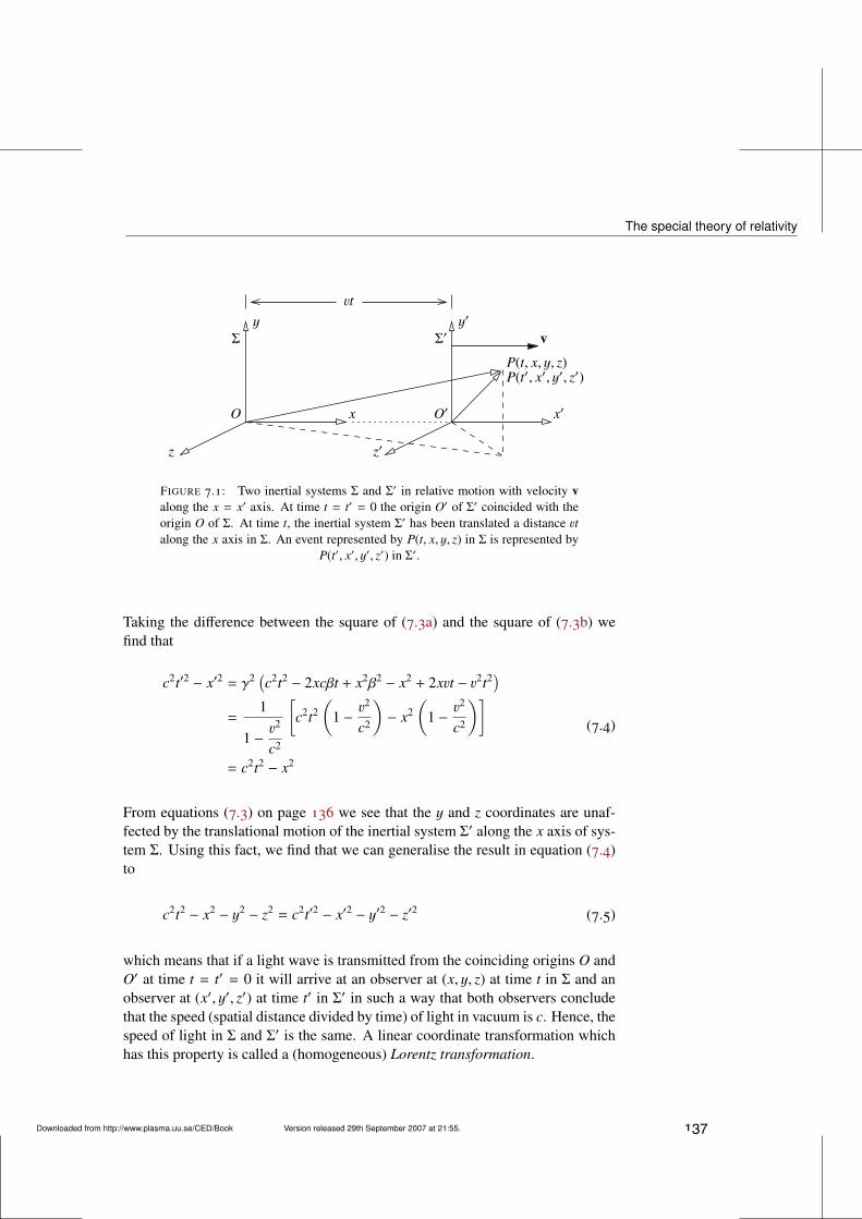
The special theory of relativity
P(t′, x′, y′, z′)
vt
P(t, x, y, z)
z′
x x′
z
O O′
Σ Σ′y y′
v
FIGURE 7.1: Two inertial systems Σ and Σ′ in relative motion with velocity valong the x = x′ axis. At time t = t′ = 0 the origin O′ of Σ′ coincided with theorigin O of Σ. At time t, the inertial system Σ′ has been translated a distance vtalong the x axis in Σ. An event represented by P(t, x, y, z) in Σ is represented by
P(t′, x′, y′, z′) in Σ′.
Taking the difference between the square of (7.3a) and the square of (7.3b) wefind that
c2t′2 − x′2 = γ2 (c2t2 − 2xcβt + x2β2 − x2 + 2xvt − v2t2)=
1
1 −v2
c2
[c2t2
(1 −
v2
c2
)− x2
(1 −
v2
c2
)]
= c2t2 − x2
(7.4)
From equations (7.3) on page 136 we see that the y and z coordinates are unaf-fected by the translational motion of the inertial system Σ′ along the x axis of sys-tem Σ. Using this fact, we find that we can generalise the result in equation (7.4)to
c2t2 − x2 − y2 − z2 = c2t′2 − x′2 − y′2 − z′2 (7.5)
which means that if a light wave is transmitted from the coinciding origins O andO′ at time t = t′ = 0 it will arrive at an observer at (x, y, z) at time t in Σ and anobserver at (x′, y′, z′) at time t′ in Σ′ in such a way that both observers concludethat the speed (spatial distance divided by time) of light in vacuum is c. Hence, thespeed of light in Σ and Σ′ is the same. A linear coordinate transformation whichhas this property is called a (homogeneous) Lorentz transformation.
Downloaded from http://www.plasma.uu.se/CED/Book Version released 29th September 2007 at 21:55. 137
7. Relativistic Electrodynamics
7.1.2 Lorentz spaceLet us introduce an ordered quadruple of real numbers, enumerated with the helpof upper indices µ = 0, 1, 2, 3, where the zeroth component is ct (c is the speedof light and t is time), and the remaining components are the components of theordinary R3 radius vector x defined in equation (M.1) on page 184:
xµ = (x0, x1, x2, x3) = (ct, x, y, z) ≡ (ct, x) (7.6)
We want to interpret this quadruple xµ as (the component form of) a radius four-vector in a real, linear, four-dimensional vector space.2 We require that this four-dimensional space be a Riemannian space, i.e., a metric space where a ‘distance’and a scalar product are defined. In this space we therefore define a metric tensor,also known as the fundamental tensor, which we denote by gµν.
Radius four-vector in contravariant and covariant form
The radius four-vector xµ = (x0, x1, x2, x3) = (ct, x), as defined in equation (7.6),is, by definition, the prototype of a contravariant vector (or, more accurately, avector in contravariant component form). To every such vector there exists a dualvector. The vector dual to xµ is the covariant vector xµ, obtained as
xµ = gµνxν (7.7)
where the upper index µ in xµ is summed over and is therefore a dummy indexand may be replaced by another dummy index ν This summation process is anexample of index contraction and is often referred to as index lowering.
Scalar product and normThe scalar product of xµ with itself in a Riemannian space is defined as
gµνxνxµ = xµxµ (7.8)
This scalar product acts as an invariant ‘distance’, or norm, in this space.To describe the physical property of Lorentz transformation invariance, de-
scribed by equation (7.5) on page 137, in mathematical language it is convenient
2The British mathematician and philosopher Alfred North Whitehead writes in his book The Conceptof Nature [43]:
‘I regret that it has been necessary for me in this lecture to administer a large dose offour-dimensional geometry. I do not apologise, because I am really not responsible for thefact that nature in its most fundamental aspect is four-dimensional. Things are what theyare. . . .’
138 Version released 29th September 2007 at 21:55. Downloaded from http://www.plasma.uu.se/CED/Book
The special theory of relativity
to perceive it as the manifestation of the conservation of the norm in a 4D Rieman-nian space. Then the explicit expression for the scalar product of xµ with itself inthis space must be
xµxµ = c2t2 − x2 − y2 − z2 (7.9)
We notice that our space will have an indefinite norm which means that we dealwith a non-Euclidean space. We call the four-dimensional space (or space-time)with this property Lorentz space and denote it L4. A corresponding real, linear 4Dspace with a positive definite norm which is conserved during ordinary rotationsis a Euclidean vector space. We denote such a space R4.
Metric tensor
By choosing the metric tensor in L4 as
gµν =
1 if µ = ν = 0−1 if µ = ν = i = j = 1, 2, 30 if µ , ν
(7.10)
or, in matrix notation,
(gµν) =
1 0 0 00 −1 0 00 0 −1 00 0 0 −1
(7.11)
i.e., a matrix with a main diagonal that has the sign sequence, or signature,+,−,−,−, the index lowering operation in our chosen flat 4D space becomesnearly trivial:
xµ = gµνxν = (ct,−x) (7.12)
Using matrix algebra, this can be writtenx0
x1
x2
x3
=
1 0 0 00 −1 0 00 0 −1 00 0 0 −1
x0
x1
x2
x3
=
x0
−x1
−x2
−x3
(7.13)
Hence, if the metric tensor is defined according to expression (7.10) the covari-ant radius four-vector xµ is obtained from the contravariant radius four-vector xµ
simply by changing the sign of the last three components. These components are
Downloaded from http://www.plasma.uu.se/CED/Book Version released 29th September 2007 at 21:55. 139
7. Relativistic Electrodynamics
referred to as the space components; the zeroth component is referred to as thetime component.
As we see, for this particular choice of metric, the scalar product of xµ withitself becomes
xµxµ = (ct, x) · (ct,−x) = c2t2 − x2 − y2 − z2 (7.14)
which indeed is the desired Lorentz transformation invariance as required by equa-tion (7.9) on page 139. Without changing the physics, one can alternatively choosea signature −,+,+,+. The latter has the advantage that the transition from 3Dto 4D becomes smooth, while it will introduce some annoying minus signs in thetheory. In current physics literature, the signature +,−,−,− seems to be the mostcommonly used one.
The L4 metric tensor equation (7.10) on page 139 has a number of interestingproperties: firstly, we see that this tensor has a trace Tr
(gµν)= −2 whereas in R4,
as in any vector space with definite norm, the trace equals the space dimension-ality. Secondly, we find, after trivial algebra, that the following relations betweenthe contravariant, covariant and mixed forms of the metric tensor hold:
gµν = gνµ (7.15a)
gµν = gµν (7.15b)
gνκgκµ = gµν = δ
µν (7.15c)
gνκgκµ = gνµ = δ
νµ (7.15d)
Here we have introduced the 4D version of the Kronecker delta δµν , a mixed four-tensor of rank 2 which fulfils
δµν = δνµ =
1 if µ = ν0 if µ , ν
(7.16)
Invariant line element and proper time
The differential distance ds between the two points xµ and xµ + dxµ in L4 can becalculated from the Riemannian metric, given by the quadratic differential form
ds2 = gµνdxνdxµ = dxµdxµ = (dx0)2 − (dx1)2 − (dx2)2 − (dx3)2 (7.17)
where the metric tensor is as in equation (7.10) on page 139. As we see, thisform is indefinite as expected for a non-Euclidean space. The square root of this
140 Version released 29th September 2007 at 21:55. Downloaded from http://www.plasma.uu.se/CED/Book
The special theory of relativity
expression is the invariant line element
ds = c dt
√√√√1 −1c2
[(dxdt
1)2
+
(dxdt
2)2
+
(dxdt
3)2]
= c dt
√1 −
1c2
[(vx)2 + (vy)2 + (vz)2
]= c dt
√1 −
v2
c2
= c dt√
1 − β2 = cdtγ= c dτ
(7.18)
where we introduced
dτ = dt/γ (7.19)
Since dτ measures the time when no spatial changes are present, it is called theproper time.
Expressing the property of the Lorentz transformation described by equa-tions (7.5) on page 137 in terms of the differential interval ds and comparingwith equation (7.17) on page 140, we find that
ds2 = c2dt2 − dx2 − dy2 − dz2 (7.20)
is invariant, i.e., remains unchanged, during a Lorentz transformation. Conversely,we may say that every coordinate transformation which preserves this differentialinterval is a Lorentz transformation.
If in some inertial system
dx2 + dy2 + dz2 < c2dt2 (7.21)
ds is a time-like interval, but if
dx2 + dy2 + dz2 > c2dt2 (7.22)
ds is a space-like interval, whereas
dx2 + dy2 + dz2 = c2dt2 (7.23)
is a light-like interval; we may also say that in this case we are on the light cone.A vector which has a light-like interval is called a null vector. The time-like,space-like or light-like aspects of an interval ds are invariant under a Lorentztransformation. I.e., it is not possible to change a time-like interval into a space-like one or vice versa via a Lorentz transformation.
Downloaded from http://www.plasma.uu.se/CED/Book Version released 29th September 2007 at 21:55. 141
7. Relativistic Electrodynamics
Four-vector fieldsAny quantity which relative to any coordinate system has a quadruple of realnumbers and transforms in the same way as the radius four-vector xµ does, iscalled a four-vector. In analogy with the notation for the radius four-vector weintroduce the notation aµ = (a0, a) for a general contravariant four-vector field inL4 and find that the ‘lowering of index’ rule, formula (7.7) on page 138, for suchan arbitrary four-vector yields the dual covariant four-vector field
aµ(xκ) = gµνaν(xκ) = (a0(xκ),−a(xκ)) (7.24)
The scalar product between this four-vector field and another one bµ(xκ) is
gµνaν(xκ)bµ(xκ) = (a0,−a) · (b0,b) = a0b0 − a · b (7.25)
which is a scalar field, i.e., an invariant scalar quantity α(xκ) which depends ontime and space, as described by xκ = (ct, x, y, z).
The Lorentz transformation matrixIntroducing the transformation matrix
(Λµν)=
γ −βγ 0 0−βγ γ 0 0
0 0 1 00 0 0 1
(7.26)
the linear Lorentz transformation (7.3) on page 136, i.e., the coordinate transfor-mation xµ → x′µ = x′µ(x0, x1, x2, x3), from one inertial system Σ to another inertialsystem Σ′ in the standard configuration, can be written
x′µ = Λµνxν (7.27)
The Lorentz groupIt is easy to show, by means of direct algebra, that two successive Lorentz trans-formations of the type in equation (7.27), and defined by the speed parameters β1
and β2, respectively, correspond to a single transformation with speed parameter
β =β1 + β2
1 + β1β2(7.28)
This means that the nonempty set of Lorentz transformations constitutes a closedalgebraic structure with a binary operation which is associative. Furthermore,one can show that this set possesses at least one identity element and at least oneinverse element. In other words, this set of Lorentz transformations constitutesa mathematical group. However tempting, we shall not make any further use ofgroup theory.
142 Version released 29th September 2007 at 21:55. Downloaded from http://www.plasma.uu.se/CED/Book
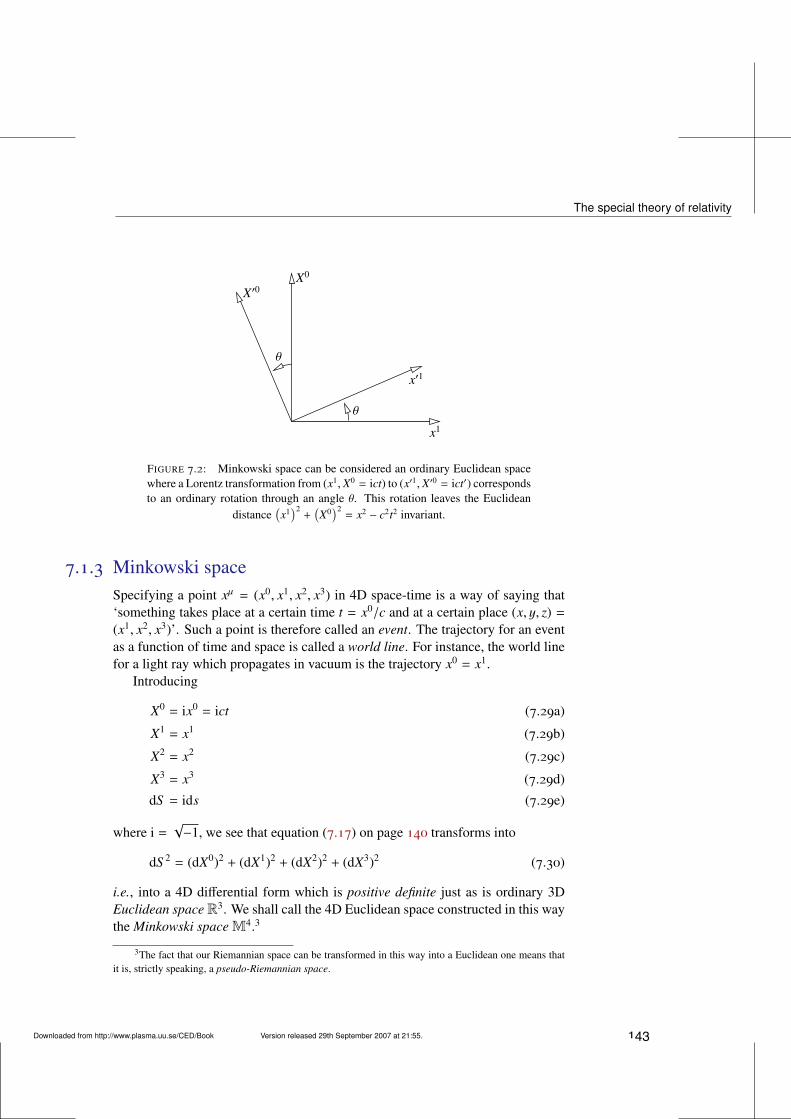
The special theory of relativity
θ
θ
X′0
x′1
x1
X0
FIGURE 7.2: Minkowski space can be considered an ordinary Euclidean spacewhere a Lorentz transformation from (x1, X0 = ict) to (x′1, X′0 = ict′) correspondsto an ordinary rotation through an angle θ. This rotation leaves the Euclidean
distance(
x1)2+(X0)2= x2 − c2t2 invariant.
7.1.3 Minkowski spaceSpecifying a point xµ = (x0, x1, x2, x3) in 4D space-time is a way of saying that‘something takes place at a certain time t = x0/c and at a certain place (x, y, z) =(x1, x2, x3)’. Such a point is therefore called an event. The trajectory for an eventas a function of time and space is called a world line. For instance, the world linefor a light ray which propagates in vacuum is the trajectory x0 = x1.
Introducing
X0 = ix0 = ict (7.29a)
X1 = x1 (7.29b)
X2 = x2 (7.29c)
X3 = x3 (7.29d)
dS = ids (7.29e)
where i =√−1, we see that equation (7.17) on page 140 transforms into
dS 2 = (dX0)2 + (dX1)2 + (dX2)2 + (dX3)2 (7.30)
i.e., into a 4D differential form which is positive definite just as is ordinary 3DEuclidean space R3. We shall call the 4D Euclidean space constructed in this waythe Minkowski space M4.3
3The fact that our Riemannian space can be transformed in this way into a Euclidean one means thatit is, strictly speaking, a pseudo-Riemannian space.
Downloaded from http://www.plasma.uu.se/CED/Book Version released 29th September 2007 at 21:55. 143
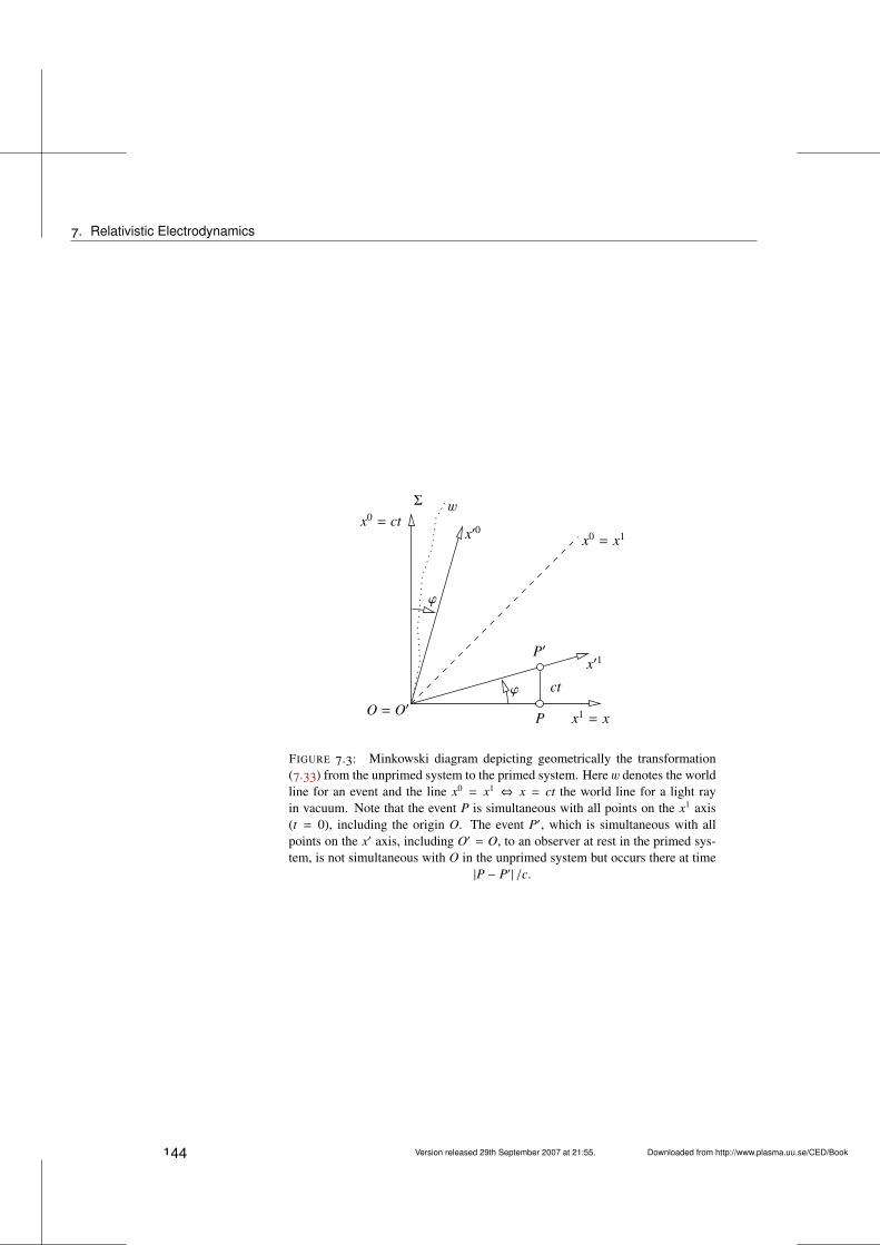
7. Relativistic Electrodynamics
x0 = ct
ct
x′1
x′0
x1 = xO = O′ϕ
P
P′
ϕ
x0 = x1
wΣ
FIGURE 7.3: Minkowski diagram depicting geometrically the transformation(7.33) from the unprimed system to the primed system. Here w denotes the worldline for an event and the line x0 = x1 ⇔ x = ct the world line for a light rayin vacuum. Note that the event P is simultaneous with all points on the x1 axis(t = 0), including the origin O. The event P′, which is simultaneous with allpoints on the x′ axis, including O′ = O, to an observer at rest in the primed sys-tem, is not simultaneous with O in the unprimed system but occurs there at time
|P − P′| /c.
144 Version released 29th September 2007 at 21:55. Downloaded from http://www.plasma.uu.se/CED/Book
The special theory of relativity
As before, it suffices to consider the simplified case where the relative motionbetween Σ and Σ′ is along the x axes. Then
dS 2 = (dX0)2 + (dX1)2 = (dX0)2 + (dx1)2 (7.31)
and we consider the X0 and X1 = x1 axes as orthogonal axes in a Euclidean space.As in all Euclidean spaces, every interval is invariant under a rotation of the X0x1
plane through an angle θ into X′0x′1:
X′0 = −x1 sin θ + X0 cos θ (7.32a)
x′1 = x1 cos θ + X0 sin θ (7.32b)
See figure 7.2 on page 143.If we introduce the angle ϕ = −iθ, often called the rapidity or the Lorentz
boost parameter, and transform back to the original space and time variables byusing equation (7.29) on page 143 backwards, we obtain
ct′ = −x sinhϕ + ct coshϕ (7.33a)
x′ = x coshϕ − ct sinhϕ (7.33b)
which are identical to the transformation equations (7.3) on page 136 if we let
sinhϕ = γβ (7.34a)
coshϕ = γ (7.34b)
tanhϕ = β (7.34c)
It is therefore possible to envisage the Lorentz transformation as an ‘ordinary’rotation in the 4D Euclidean space M4. Such a rotation in M4 corresponds to acoordinate change in L4 as depicted in figure 7.3 on page 144. equation (7.28)on page 142 for successive Lorentz transformation then corresponds to the tanhaddition formula
tanh(ϕ1 + ϕ2) =tanhϕ1 + tanhϕ2
1 + tanhϕ1 tanhϕ2(7.35)
The use of ict and M4, which leads to the interpretation of the Lorentz trans-formation as an ‘ordinary’ rotation, may, at best, be illustrative, but is not veryphysical. Besides, if we leave the flat L4 space and enter the curved space ofgeneral relativity, the ‘ict’ trick will turn out to be an impasse. Let us thereforeimmediately return to L4 where all components are real valued.
Downloaded from http://www.plasma.uu.se/CED/Book Version released 29th September 2007 at 21:55. 145
7. Relativistic Electrodynamics
7.2 Covariant classical mechanicsThe invariance of the differential ‘distance’ ds in L4, and the associated differ-ential proper time dτ [see equation (7.18) on page 141] allows us to define thefour-velocity
uµ =dxdτ
µ
= γ(c, v) =
c√1 − v2
c2
,v√
1 − v2
c2
= (u0,u) (7.36)
which, when multiplied with the scalar invariant m0 yields the four-momentum
pµ = m0dxdτ
µ
= m0γ(c, v) =
m0c√1 − v2
c2
,m0v√1 − v2
c2
= (p0,p) (7.37)
From this we see that we can write
p = mv (7.38)
where
m = γm0 =m0√1 − v2
c2
(7.39)
We can interpret this such that the Lorentz covariance implies that the mass-liketerm in the ordinary 3D linear momentum is not invariant. A better way to lookat this is that p = mv = γm0v is the covariantly correct expression for the kineticthree-momentum.
Multiplying the zeroth (time) component of the four-momentum pµ with thescalar invariant c, we obtain
cp0 = γm0c2 =m0c2√1 − v2
c2
= mc2 (7.40)
Since this component has the dimension of energy and is the result of a covariantdescription of the motion of a particle with its kinetic momentum described bythe spatial components of the four-momentum, equation (7.37), we interpret cp0
as the total energy E. Hence,
cpµ = (cp0, cp) = (E, cp) (7.41)
146 Version released 29th September 2007 at 21:55. Downloaded from http://www.plasma.uu.se/CED/Book
Covariant classical electrodynamics
Scalar multiplying this four-vector with itself, we obtain
cpµcpµ = c2gµνpνpµ = c2[(p0)2 − (p1)2 − (p2)2 − (p3)2]
= (E,−cp) · (E, cp) = E2 − c2p2
=(m0c2)2
1 − v2
c2
(1 −
v2
c2
)= (m0c2)2
(7.42)
Since this is an invariant, this equation holds in any inertial frame, particularly inthe frame where p = 0 and there we have
E = m0c2 (7.43)
This is probably the most famous formula in physics history.
7.3 Covariant classical electrodynamicsLet us consider a charge density which in its rest inertial system is denoted by ρ0.The four-vector (in contravariant component form)
jµ = ρ0dxµ
dτ= ρ0uµ = ρ0γ(c, v) = (ρc, ρv) (7.44)
where we introduced
ρ = γρ0 (7.45)
is called the four-current.The contravariant form of the four-del operator ∂µ = ∂/∂xµ is defined in
equation (M.37) on page 190 and its covariant counterpart ∂µ = ∂/∂xµ in equa-tion (M.38) on page 190, respectively. As is shown in example M.5 on page 199,the d’Alembert operator is the scalar product of the four-del with itself:
2 = ∂µ∂µ = ∂µ∂µ =
1c2
∂2
∂t2 − ∇2 (7.46)
Since it has the characteristics of a four-scalar, the d’Alembert operator is invariantand, hence, the homogeneous wave equation 2 f (t, x) = 0 is Lorentz covariant.
7.3.1 The four-potentialIf we introduce the four-potential
Aµ =
(φ
c,A)
(7.47)
Downloaded from http://www.plasma.uu.se/CED/Book Version released 29th September 2007 at 21:55. 147
7. Relativistic Electrodynamics
where φ is the scalar potential and A the vector potential, defined in section 3.3on page 44, we can write the uncoupled inhomogeneous wave equations, equa-tions (3.16) on page 47, in the following compact (and covariant) way:
2Aµ = µ0 jµ (7.48)
With the help of the above, we can formulate our electrodynamic equationscovariantly. For instance, the covariant form of the equation of continuity, equa-tion (1.23) on page 10 is
∂µ jµ = 0 (7.49)
and the Lorenz-Lorentz gauge condition, equation (3.15) on page 47, can be writ-ten
∂µAµ = 0 (7.50)
The gauge transformations (3.11) on page 46 in covariant form are
Aµ 7→ A′µ = Aµ + ∂µΓ(xν) (7.51)
If only one dimension Lorentz contracts (for instance, due to relative motionalong the x direction), a 3D spatial volume element transforms according to
dV = d3x =1γ
dV0 = dV0
√1 − β2 = dV0
√1 −
v2
c2 (7.52)
where dV0 denotes the volume element as measured in the rest system, then fromequation (7.45) on page 147 we see that
ρdV = ρ0dV0 (7.53)
i.e., the charge in a given volume is conserved. We can therefore conclude thatthe elementary charge is a universal constant.
7.3.2 The Liénard-Wiechert potentialsLet us now solve the the inhomogeneous wave equations (3.16) on page 47 invacuum for the case of a well-localised charge q′ at a source point defined by theradius four-vector x′µ ≡ (x′0 = ct′, x′1, x′2, x′3). The field point (observation point)is denoted by the radius four-vector xµ = (x0 = ct, x1, x2, x3).
In the rest system we know that the solution is simply
(Aµ)0 =
(φ
c,A)
v=0=
(q′
4πε0
1c |x − x′|0
, 0)
(7.54)
148 Version released 29th September 2007 at 21:55. Downloaded from http://www.plasma.uu.se/CED/Book
Covariant classical electrodynamics
where |x − x′|0 is the usual distance from the source point to the field point, eval-uated in the rest system (signified by the index ‘0’).
Let us introduce the relative radius four-vector between the source point andthe field point:
Rµ = xµ − x′µ = (c(t − t′), x − x′) (7.55)
Scalar multiplying this relative four-vector with itself, we obtain
RµRµ = (c(t − t′), x − x′) · (c(t − t′),−(x − x′)) = c2(t − t′)2 −∣∣x − x′
∣∣2(7.56)
We know that in vacuum the signal (field) from the charge q′ at x′µ propagatesto xµ with the speed of light c so that∣∣x − x′
∣∣ = c(t − t′) (7.57)
Inserting this into equation (7.56) above, we see that
RµRµ = 0 (7.58)
or that equation (7.55) can be written
Rµ = (∣∣x − x′
∣∣ , x − x′) (7.59)
Now we want to find the correspondence to the rest system solution, equa-tion (7.54) on page 148, in an arbitrary inertial system. We note from equa-tion (7.36) on page 146 that in the rest system
(uµ)0 =
c√1 − v2
c2
,v√
1 − v2
c2
v=0
= (c, 0) (7.60)
and
(Rµ)0 = (∣∣x − x′
∣∣ , x − x′)0 = (∣∣x − x′
∣∣0 , (x − x′)0) (7.61)
As all scalar products, uµRµ is invariant, which means that we can evaluate itin any inertial system and it will have the same value in all other inertial systems.If we evaluate it in the rest system the result is:
uµRµ =(uµRµ
)0 = (uµ)0(Rµ)0
= (c, 0) · (∣∣x − x′
∣∣0 ,−(x − x′)0) = c
∣∣x − x′∣∣0
(7.62)
Downloaded from http://www.plasma.uu.se/CED/Book Version released 29th September 2007 at 21:55. 149
7. Relativistic Electrodynamics
We therefore see that the expression
Aµ =q′
4πε0
uµ
cuνRν(7.63)
subject to the condition RµRµ = 0 has the proper transformation properties (propertensor form) and reduces, in the rest system, to the solution equation (7.54) onpage 148. It is therefore the correct solution, valid in any inertial system.
According to equation (7.36) on page 146 and equation (7.59) on page 149
uνRν = γ(c, v) ·(∣∣x − x′
∣∣ ,−(x − x′))= γ
(c∣∣x − x′
∣∣ − v · (x − x′))
(7.64)
Generalising expression (7.1) on page 136 to vector form:
β = β vdef≡
vc
(7.65)
and introducing
sdef≡∣∣x − x′
∣∣ − v · (x − x′)c
≡∣∣x − x′
∣∣ − β · (x − x′) (7.66)
we can write
uνRν = γcs (7.67)
and
uµ
cuνRν=
(1cs,
vc2s
)(7.68)
from which we see that the solution (7.63) can be written
Aµ(xκ) =q′
4πε0
(1cs,
vc2s
)=
(φ
c,A)
(7.69)
where in the last step the definition of the four-potential, equation (7.47) on page 147,was used. Writing the solution in the ordinary 3D way, we conclude that for a verylocalised charge volume, moving relative an observer with a velocity v, the scalarand vector potentials are given by the expressions
φ(t, x) =q′
4πε0
1s=
q′
4πε0
1|x − x′| − β · (x − x′)
(7.70a)
A(t, x) =q′
4πε0c2
vs=
q′
4πε0c2
v|x − x′| − β · (x − x′)
(7.70b)
These potentials are the Liénard-Wiechert potentials that we derived in a morecomplicated and restricted way in subsection 6.3.1 on page 98.
150 Version released 29th September 2007 at 21:55. Downloaded from http://www.plasma.uu.se/CED/Book
Covariant classical electrodynamics
7.3.3 The electromagnetic field tensorConsider a vectorial (cross) product c between two ordinary vectors a and b:
c = a × b = εi jkaib j xk
= (a2b3 − a3b2)x1 + (a3b1 − a1b3)x2 + (a1b2 − a2b1)x3(7.71)
We notice that the kth component of the vector c can be represented as
ck = aib j − a jbi = ci j = −c ji, i, j , k (7.72)
In other words, the pseudovector c = a×b can be considered as an antisymmetrictensor of rank two. The same is true for the curl operator ∇× operating on a polarvector. For instance, the Maxwell equation
∇ × E = −∂B∂t
(7.73)
can in this tensor notation be written
∂E j
∂xi −∂Ei
∂x j = −∂Bi j
∂t(7.74)
We know from chapter 3 that the fields can be derived from the electromag-netic potentials in the following way:
B = ∇ × A (7.75a)
E = −∇φ −∂A∂t
(7.75b)
In component form, this can be written
Bi j =∂A j
∂xi −∂Ai
∂x j = ∂iA j − ∂ jAi (7.76a)
Ei = −∂φ
∂xi −∂Ai
∂t= −∂iφ − ∂tAi (7.76b)
From this, we notice the clear difference between the axial vector (pseudovector)B and the polar vector (‘ordinary vector’) E.
Our goal is to express the electric and magnetic fields in a tensor form wherethe components are functions of the covariant form of the four-potential, equa-tion (7.47) on page 147:
Aµ =
(φ
c,A)
(7.77)
Downloaded from http://www.plasma.uu.se/CED/Book Version released 29th September 2007 at 21:55. 151
7. Relativistic Electrodynamics
Inspection of (7.77) and equation (7.76) on page 151 makes it natural to definethe four-tensor
Fµν =∂Aν
∂xµ−∂Aµ
∂xν= ∂µAν − ∂νAµ (7.78)
This anti-symmetric (skew-symmetric), four-tensor of rank 2 is called the electro-magnetic field tensor. In matrix representation, the contravariant field tensor canbe written
(Fµν) =
0 −Ex/c −Ey/c −Ez/c
Ex/c 0 −Bz ByEy/c Bz 0 −Bx
Ez/c −By Bx 0
(7.79)
We note that the field tensor is a sort of four-dimensional curl of the four-potentialvector Aµ.
The covariant field tensor is obtained from the contravariant field tensor in theusual manner by index lowering
Fµν = gµκgνλFκλ = ∂µAν − ∂νAµ (7.80)
which in matrix representation becomes
(Fµν
)=
0 Ex/c Ey/c Ez/c
−Ex/c 0 −Bz By−Ey/c Bz 0 −Bx
−Ez/c −By Bx 0
(7.81)
Comparing formula (7.81) above with formula (7.79) we see that the covariantfield tensor is obtained from the contravariant one by a transformation E→ −E.
That the two Maxwell source equations can be written
∂µFµν = µ0 jν (7.82)
is immediately observed by explicitly solving this covariant equation. Settingν = 0, corresponding to the first/leftmost column in the matrix representation ofthe covariant component form of the electromagnetic field tensor, Fµν, i.e., equa-tion (7.79) above, we see that
∂F00
∂x0 +∂F10
∂x1 +∂F20
∂x2 +∂F30
∂x3 = 0 +1c
(∂Ex
∂x+∂Ey
∂y+∂Ez
∂z
)=
1c∇ · E = µ0 j0 = µ0cρ
(7.83)
152 Version released 29th September 2007 at 21:55. Downloaded from http://www.plasma.uu.se/CED/Book
Covariant classical electrodynamics
or, equivalently (recalling that ε0µ0 = 1/c2),
∇ · E =ρ
ε0(7.84)
which we recognise at the Maxwell source equation for the electric field, equa-tion (1.45a) on page 15.
For ν = 1 (the second column in equation (7.79) on page 152), equation (7.82)on page 152 yields
∂F01
∂x0 +∂F11
∂x1 +∂F21
∂x2 +∂F31
∂x3 = −1c2
∂Ex
∂t+ 0 +
∂Bz
∂y−∂By∂z= µ0 j1 = µ0ρvx
(7.85)
This result can be rewritten as∂Bz
∂y−∂By∂z− ε0µ0
∂Ex
∂t= µ0 jx (7.86)
or, equivalently, as
(∇ × B)x = µ0 jx + ε0µ0∂Ex
∂t(7.87)
and similarly for ν = 2, 3. In summary, we can write the result in three-vectorform as
∇ × B = µ0j(t, x) + ε0µ0∂E∂t
(7.88)
which we recognise as the Maxwell source equation for the magnetic field, equa-tion (1.45d) on page 15.
With the help of the fully antisymmetric rank-4 pseudotensor
εµνκλ =
1 if µ, ν, κ, λ is an even permutation of 0,1,2,30 if at least two of µ, ν, κ, λ are equal−1 if µ, ν, κ, λ is an odd permutation of 0,1,2,3
(7.89)
which can be viewed as a generalisation of the Levi-Civita tensor, formula (M.18)on page 187, we can introduce the dual electromagnetic tensor
?Fµν = εµνκλFκλ (7.90)
In matrix form the dual field tensor is
(?Fµν
)=
0 −cBx −cBy −cBz
cBx 0 Ez −Ey
cBy −Ez 0 Ex
cBz Ey −Ex 0
(7.91)
Downloaded from http://www.plasma.uu.se/CED/Book Version released 29th September 2007 at 21:55. 153
7. Relativistic Electrodynamics
i.e., the dual field tensor is obtained from the ordinary field tensor by the dualitytransformation E→ c2B and B→ −E.
The covariant form of the two Maxwell field equations
∇ × E = −∂B∂t
(7.92)
∇ · B = 0 (7.93)
can then be written
∂µ?Fµν = 0 (7.94)
Explicit evaluation shows that this corresponds to (no summation!)
∂κFµν + ∂µFνκ + ∂νFκµ = 0 (7.95)
sometimes referred to as the Jacobi identity. Hence, equation (7.82) on page 152and equation (7.95) constitute Maxwell’s equations in four-dimensional formal-ism.
It is interesting to note that equation (7.82) on page 152 and
∂µ?Fµν = µ0 jνm (7.96)
where jm is the magnetic four-current, represent the covariant form of Dirac’ssymmetrised Maxwell equations (1.50) on page 16.
7.4 Bibliography[1] J. AHARONI, The Special Theory of Relativity, second, revised ed., Dover Publica-
tions, Inc., New York, 1985, ISBN 0-486-64870-2.
[2] A. O. BARUT, Electrodynamics and Classical Theory of Fields and Particles, Dover Pub-lications, Inc., New York, NY, 1980, ISBN 0-486-64038-8.
[3] R. BECKER, Electromagnetic Fields and Interactions, Dover Publications, Inc.,New York, NY, 1982, ISBN 0-486-64290-9.
[4] D. BOHM, The Special Theory of Relativity, Routledge, New York, NY, 1996, ISBN 0-415-14809-X.
[5] W. T. GRANDY, Introduction to Electrodynamics and Radiation, Academic Press,New York and London, 1970, ISBN 0-12-295250-2.
154 Version released 29th September 2007 at 21:55. Downloaded from http://www.plasma.uu.se/CED/Book
Bibliography
[6] L. D. LANDAU AND E. M. LIFSHITZ, The Classical Theory of Fields, fourth revisedEnglish ed., vol. 2 of Course of Theoretical Physics, Pergamon Press, Ltd., Oxford . . . ,1975, ISBN 0-08-025072-6.
[7] F. E. LOW, Classical Field Theory, John Wiley & Sons, Inc., New York, NY . . . , 1997,ISBN 0-471-59551-9.
[8] H. MUIRHEAD, The Special Theory of Relativity, The Macmillan Press Ltd., London,Beccles and Colchester, 1973, ISBN 333-12845-1.
[9] C. MØLLER, The Theory of Relativity, second ed., Oxford University Press, Glasgow . . . ,1972.
[10] W. K. H. PANOFSKY AND M. PHILLIPS, Classical Electricity and Magnetism, second ed.,Addison-Wesley Publishing Company, Inc., Reading, MA . . . , 1962, ISBN 0-201-05702-6.
[11] J. J. SAKURAI, Advanced Quantum Mechanics, Addison-Wesley Publishing Com-pany, Inc., Reading, MA . . . , 1967, ISBN 0-201-06710-2.
[12] B. SPAIN, Tensor Calculus, third ed., Oliver and Boyd, Ltd., Edinburgh and London,1965, ISBN 05-001331-9.
[13] A. N. WHITEHEAD, Concept of Nature, Cambridge University Press, Cambridge . . . ,1920, ISBN 0-521-09245-0.
Downloaded from http://www.plasma.uu.se/CED/Book Version released 29th September 2007 at 21:55. 155

Downloaded from http://www.plasma.uu.se/CED/Book Version released 29th September 2007 at 21:55.
8Electromagnetic
Fields andParticles
In previous chapters, we calculated the electromagnetic fields and potentials fromarbitrary, but prescribed distributions of charges and currents. In this chapter westudy the general problem of interaction between electric and magnetic fields andelectrically charged particles. The analysis is based on Lagrangian and Hamil-tonian methods, is fully covariant, and yields results which are relativisticallycorrect.
8.1 Charged particles in an electromagnetic fieldWe first establish a relativistically correct theory describing the motion of chargedparticles in prescribed electric and magnetic fields. From these equations we maythen calculate the charged particle dynamics in the most general case.
8.1.1 Covariant equations of motionWe will show that for our problem we can derive the correct equations of mo-tion by using in four-dimensional L4 a function with similar properties as a La-grange function in 3D and then apply a variational principle. We will also showthat we can find a Hamiltonian-type function in 4D and solve the correspondingHamilton-type equations to obtain the correct covariant formulation of classicalelectrodynamics.
157
8. Electromagnetic Fields and Particles
Lagrange formalismLet us now introduce a generalised action
S4 =
∫L4(xµ, uµ) dτ (8.1)
where dτ is the proper time defined via equation (7.18) on page 141, and L4 actsas a kind of generalisation to the common 3D Lagrangian so that the variationalprinciple
δS4 = δ
∫ τ1
τ0
L4(xµ, uµ) dτ = 0 (8.2)
with fixed endpoints τ0, τ1 is fulfilled. We require that L4 is a scalar invariantwhich does not contain higher than the second power of the four-velocity uµ inorder that the equations of motion be linear.
According to formula (M.48) on page 192 the ordinary 3D Lagrangian is thedifference between the kinetic and potential energies. A free particle has onlykinetic energy. If the particle mass is m0 then in 3D the kinetic energy is m0v
2/2.This suggests that in 4D the Lagrangian for a free particle should be
Lfree4 =
12
m0uµuµ (8.3)
For an interaction with the electromagnetic field we can introduce the interactionwith the help of the four-potential given by equation (7.77) on page 151 in thefollowing way
L4 =12
m0uµuµ + quµAµ(xν) (8.4)
We call this the four-Lagrangian and shall now show how this function, togetherwith the variation principle, formula (8.2), yields covariant results which are phys-ically correct.
The variation principle (8.2) with the 4D Lagrangian (8.4) inserted, leads to
δS4 = δ
∫ τ1
τ0
(m0
2uµuµ + quµAµ
)dτ
=
∫ τ1
τ0
[m0
2∂(uµuµ)∂uµ
δuµ + q(
Aµδuµ + uµ∂Aµ
∂xνδxν)]
dτ
=
∫ τ1
τ0
[m0uµδuµ + q
(Aµδuµ + uµ∂νAµδxν
)]dτ = 0
(8.5)
According to equation (7.36) on page 146, the four-velocity is
uµ =dxdτ
µ
(8.6)
158 Version released 29th September 2007 at 21:55. Downloaded from http://www.plasma.uu.se/CED/Book
Charged particles in an electromagnetic field
which means that we can write the variation of uµ as a total derivative with respectto τ :
δuµ = δ(
dxdτ
µ)=
ddτ
(δxµ) (8.7)
Inserting this into the first two terms in the last integral in equation (8.5) onpage 158, we obtain
δS4 =
∫ τ1
τ0
(m0uµ
ddτ
(δxµ) + qAµddτ
(δxµ) + quµ∂νAµδxν)
dτ (8.8)
Partial integration in the two first terms in the right hand member of (8.8) gives
δS4 =
∫ τ1
τ0
(−m0
duµdτ
δxµ − qdAµ
dτδxµ + quµ∂νAµδxν
)dτ (8.9)
where the integrated parts do not contribute since the variations at the endpointsvanish. A change of irrelevant summation index from µ to ν in the first two termsof the right hand member of (8.9) yields, after moving the ensuing common factorδxν outside the parenthesis, the following expression:
δS4 =
∫ τ1
τ0
(−m0
duνdτ− q
dAν
dτ+ quµ∂νAµ
)δxν dτ (8.10)
Applying well-known rules of differentiation and the expression (7.36) for thefour-velocity, we can express dAν/dτ as follows:
dAν
dτ=∂Aν
∂xµdxµ
dτ= ∂µAνuµ (8.11)
By inserting this expression (8.11) into the second term in right-hand member ofequation (8.10) above, and noting the common factor quµ of the resulting termand the last term, we obtain the final variational principle expression
δS4 =
∫ τ1
τ0
[−m0
duνdτ+ quµ
(∂νAµ − ∂µAν
)]δxν dτ (8.12)
Since, according to the variational principle, this expression shall vanish and δxν
is arbitrary between the fixed end points τ0 and τ1, the expression inside[ ]
inthe integrand in the right hand member of equation (8.12) must vanish. In otherwords, we have found an equation of motion for a charged particle in a prescribedelectromagnetic field:
m0duνdτ= quµ
(∂νAµ − ∂µAν
)(8.13)
Downloaded from http://www.plasma.uu.se/CED/Book Version released 29th September 2007 at 21:55. 159
8. Electromagnetic Fields and Particles
With the help of formula (7.80) on page 152 for the covariant component form ofthe field tensor, we can express this equation in terms of the electromagnetic fieldtensor in the following way:
m0duνdτ= quµFνµ (8.14)
This is the sought-for covariant equation of motion for a particle in an electro-magnetic field. It is often referred to as the Minkowski equation. As the readercan easily verify, the spatial part of this 4-vector equation is the covariant (rela-tivistically correct) expression for the Newton-Lorentz force equation.
Hamiltonian formalismThe usual Hamilton equations for a 3D space are given by equation (M.55) onpage 193 in appendix M. These six first-order partial differential equations are
∂H∂pi=
dqi
dt(8.15a)
∂H∂qi= −
dpi
dt(8.15b)
where H(pi, qi, t) = piqi − L(qi, qi, t) is the ordinary 3D Hamiltonian, qi is a gen-eralised coordinate and pi is its canonically conjugate momentum.
We seek a similar set of equations in 4D space. To this end we introduce acanonically conjugate four-momentum pµ in an analogous way as the ordinary3D conjugate momentum:
pµ =∂L4
∂uµ(8.16)
and utilise the four-velocity uµ, as given by equation (7.36) on page 146, to definethe four-Hamiltonian
H4 = pµuµ − L4 (8.17)
With the help of these, the radius four-vector xµ, considered as the generalisedfour-coordinate, and the invariant line element ds, defined in equation (7.18) onpage 141, we introduce the following eight partial differential equations:
∂H4
∂pµ=
dxµdτ
(8.18a)
∂H4
∂xµ= −
dpµdτ
(8.18b)
160 Version released 29th September 2007 at 21:55. Downloaded from http://www.plasma.uu.se/CED/Book
Charged particles in an electromagnetic field
which form the four-dimensional Hamilton equations.Our strategy now is to use equation (8.16) on page 160 and equations (8.18) on
page 160 to derive an explicit algebraic expression for the canonically conjugatemomentum four-vector. According to equation (7.41) on page 146, c times a four-momentum has a zeroth (time) component which we can identify with the totalenergy. Hence we require that the component p0 of the conjugate four-momentumvector defined according to equation (8.16) on page 160 be identical to the ordi-nary 3D Hamiltonian H divided by c and hence that this cp0 solves the Hamiltonequations, equations (8.15) on page 160. This later consistency check is left as anexercise to the reader.
Using the definition of H4, equation (8.17) on page 160, and the expressionfor L4, equation (8.4) on page 158, we obtain
H4 = pµuµ − L4 = pµuµ −12
m0uµuµ − quµAµ(xν) (8.19)
Furthermore, from the definition (8.16) of the canonically conjugate four-momentumpµ, we see that
pµ =∂L4
∂uµ=
∂
∂uµ
(12
m0uµuµ + quµAµ(xν))= m0uµ + qAµ (8.20)
Inserting this into (8.19), we obtain
H4 = m0uµuµ + qAµuµ −12
m0uµuµ − quµAµ(xν) =12
m0uµuµ (8.21)
Since the four-velocity scalar-multiplied by itself is uµuµ = c2, we clearly seefrom equation (8.21) that H4 is indeed a scalar invariant, whose value is simply
H4 =m0c2
2(8.22)
However, at the same time (8.20) provides the algebraic relationship
uµ =1
m0(pµ − qAµ) (8.23)
and if this is used in (8.21) to eliminate uµ, one gets
H4 =m0
2
(1
m0(pµ − qAµ)
1m0
(pµ − qAµ
))=
12m0
(pµ − qAµ)(
pµ − qAµ
)=
12m0
(pµpµ − 2qAµpµ + q2AµAµ
) (8.24)
Downloaded from http://www.plasma.uu.se/CED/Book Version released 29th September 2007 at 21:55. 161
8. Electromagnetic Fields and Particles
That this four-Hamiltonian yields the correct covariant equation of motion canbe seen by inserting it into the four-dimensional Hamilton’s equations (8.18) andusing the relation (8.23):
∂H4
∂xµ= −
qm0
(pν − qAν)∂Aν
∂xµ
= −q
m0m0uν
∂Aν
∂xµ
= −quν∂Aν
∂xµ
= −dpµdτ= −m0
duµdτ− q
∂Aµ
∂xνuν
(8.25)
where in the last step equation (8.20) on page 161 was used. Rearranging terms,and using equation (7.80) on page 152, we obtain
m0duµdτ= quν
(∂µAν − ∂νAµ
)= quνFµν (8.26)
which is identical to the covariant equation of motion equation (8.14) on page 160.We can then safely conclude that the Hamiltonian in question is correct.
Recalling expression (7.47) on page 147 and representing the canonically con-jugate four-momentum as pµ = (p0,p), we obtain the following scalar products:
pµpµ = (p0)2 − (p)2 (8.27a)
Aµpµ =1cφp0 − (p · A) (8.27b)
AµAµ =1c2φ
2 − (A)2 (8.27c)
Inserting these explicit expressions into equation (8.24) on page 161, and using thefact that for H4 is equal to the scalar value m0c2/2, as derived in equation (8.22)on page 161, we obtain the equation
m0c2
2=
12m0
[(p0)2 − (p)2 −
2c
qφp0 + 2q(p · A) +q2
c2 φ2 − q2(A)2
](8.28)
which is the second order algebraic equation in p0:
(p0)2 −2qcφp0 −
[(p)2 − 2qp · A + q2(A)2]︸ ︷︷ ︸
(p−qA)2
+q2
c2 φ2 − m2
0c2 = 0 (8.29)
with two possible solutions
p0 =qcφ ±
√(p − qA)2 + m2
0c2 (8.30)
162 Version released 29th September 2007 at 21:55. Downloaded from http://www.plasma.uu.se/CED/Book
Covariant field theory
Since the zeroth component (time component) p0 of a four-momentum vector pµ
multiplied by c represents the energy [cf. equation (7.41) on page 146], the posi-tive solution in equation (8.30) on page 162 must be identified with the ordinaryHamilton function H divided by c. Consequently,
H ≡ cp0 = qφ + c√
(p − qA)2 + m20c2 (8.31)
is the ordinary 3D Hamilton function for a charged particle moving in scalar andvector potentials associated with prescribed electric and magnetic fields.
The ordinary Lagrange and Hamilton functions L and H are related to eachother by the 3D transformation [cf. the 4D transformation (8.17) between L4 andH4]
L = p · v − H (8.32)
Using the explicit expressions (equation (8.31) above) and (equation (8.32)), weobtain the explicit expression for the ordinary 3D Lagrange function
L = p · v − qφ − c√
(p − qA)2 + m20c2 (8.33)
and if we make the identification
p − qA =m0v√1 − v2
c2
= mv (8.34)
where the quantity mv is the usual kinetic momentum, we can rewrite this expres-sion for the ordinary Lagrangian as follows:
L = qA · v + mv2 − qφ − c√
m2v2 + m20c2
= mv2 − q(φ − A · v) − mc2 = −qφ + qA · v − m0c2
√1 −
v2
c2
(8.35)
What we have obtained is the relativistically correct (covariant) expression forthe Lagrangian describing the motion of a charged particle in scalar and vectorpotentials associated with prescribed electric and magnetic fields.
8.2 Covariant field theorySo far, we have considered two classes of problems. Either we have calculatedthe fields from given, prescribed distributions of charges and currents, or we have
Downloaded from http://www.plasma.uu.se/CED/Book Version released 29th September 2007 at 21:55. 163
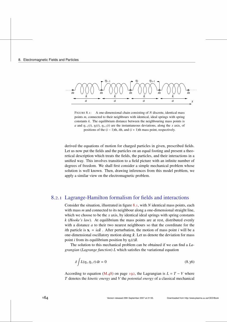
8. Electromagnetic Fields and Particles
kk
ηi+1ηiηi−1
kkm
aaa
m
x
mmm
a
FIGURE 8.1: A one-dimensional chain consisting of N discrete, identical masspoints m, connected to their neighbours with identical, ideal springs with springconstants k. The equilibrium distance between the neighbouring mass points isa and ηi−1(t), ηi(t), ηi+1(t) are the instantaneous deviations, along the x axis, of
positions of the (i − 1)th, ith, and (i + 1)th mass point, respectively.
derived the equations of motion for charged particles in given, prescribed fields.Let us now put the fields and the particles on an equal footing and present a theo-retical description which treats the fields, the particles, and their interactions in aunified way. This involves transition to a field picture with an infinite number ofdegrees of freedom. We shall first consider a simple mechanical problem whosesolution is well known. Then, drawing inferences from this model problem, weapply a similar view on the electromagnetic problem.
8.2.1 Lagrange-Hamilton formalism for fields and interactionsConsider the situation, illustrated in figure 8.1, with N identical mass points, eachwith mass m and connected to its neighbour along a one-dimensional straight line,which we choose to be the x axis, by identical ideal springs with spring constantsk (Hooke’s law). At equilibrium the mass points are at rest, distributed evenlywith a distance a to their two nearest neighbours so that the coordinate for theith particle is xi = iax . After perturbation, the motion of mass point i will be aone-dimensional oscillatory motion along x. Let us denote the deviation for masspoint i from its equilibrium position by ηi(t)x.
The solution to this mechanical problem can be obtained if we can find a La-grangian (Lagrange function) L which satisfies the variational equation
δ
∫L(ηi, ηi, t) dt = 0 (8.36)
According to equation (M.48) on page 192, the Lagrangian is L = T − V whereT denotes the kinetic energy and V the potential energy of a classical mechanical
164 Version released 29th September 2007 at 21:55. Downloaded from http://www.plasma.uu.se/CED/Book
Covariant field theory
system with conservative forces. In our case the Lagrangian is
L =12
N
∑i=1
[mη2
i − k(ηi+1 − ηi)2] (8.37)
Let us write the Lagrangian, as given by equation (8.37), in the following way:
L =N
∑i=1
aLi (8.38)
Here,
Li =12
[maη2
i − ka(ηi+1 − ηi
a
)2]
(8.39)
is the so called linear Lagrange density. If we now let N → ∞ and, at thesame time, let the springs become infinitesimally short according to the followingscheme:
a→ dx (8.40a)ma→
dmdx= µ linear mass density (8.40b)
ka→ Y Young’s modulus (8.40c)ηi+1 − ηi
a→
∂η
∂x(8.40d)
we obtain
L =∫
L dx (8.41)
where
L
(η,∂η
∂t,∂η
∂x, t)=
12
[µ
(∂η
∂t
)2
− Y(∂η
∂x
)2]
(8.42)
Notice how we made a transition from a discrete description, in which the masspoints were identified by a discrete integer variable i = 1, 2, . . . ,N, to a continu-ous description, where the infinitesimal mass points were instead identified by acontinuous real parameter x, namely their position along x.
A consequence of this transition is that the number of degrees of freedom forthe system went from the finite number N to infinity! Another consequence isthat L has now become dependent also on the partial derivative with respect tox of the ‘field coordinate’ η. But, as we shall see, the transition is well worth the
Downloaded from http://www.plasma.uu.se/CED/Book Version released 29th September 2007 at 21:55. 165
8. Electromagnetic Fields and Particles
cost because it allows us to treat all fields, be it classical scalar or vectorial fields,or wave functions, spinors and other fields that appear in quantum physics, on anequal footing.
Under the assumption of time independence and fixed endpoints, the variationprinciple (8.36) on page 164 yields:
δ
∫L dt
= δ
∫∫L
(η,∂η
∂t,∂η
∂x
)dx dt
=
∫∫ ∂L∂η
δη +∂L
∂(∂η∂t
) δ(∂η∂t
)+
∂L
∂(∂η∂x
) δ(∂η∂x
) dx dt
= 0
(8.43)
The last integral can be integrated by parts. This results in the expression
∫∫ ∂L∂η−∂
∂t
∂L
∂(∂η∂t
) − ∂
∂x
∂L
∂(∂η∂x
) δη dx dt = 0 (8.44)
where the variation is arbitrary (and the endpoints fixed). This means that theintegrand itself must vanish. If we introduce the functional derivative
δL
δη=∂L
∂η−∂
∂x
∂L
∂(∂η∂x
) (8.45)
we can express this as
δL
δη−∂
∂t
∂L
∂(∂η∂t
) = 0 (8.46)
which is the one-dimensional Euler-Lagrange equation.Inserting the linear mass point chain Lagrangian density, equation (8.42) on
page 165, into equation (8.46) above, we obtain the equation of motion for ourone-dimensional linear mechanical structure. It is:
µ∂2η
∂t2 − Y∂2η
∂x2 =
(µ
Y∂2
∂t2 −∂2
∂x2
)η = 0 (8.47)
i.e., the one-dimensional wave equation for compression waves which propagatewith phase speed vφ =
√Y/µ along the linear structure.
166 Version released 29th September 2007 at 21:55. Downloaded from http://www.plasma.uu.se/CED/Book
Covariant field theory
A generalisation of the above 1D results to a three-dimensional continuum isstraightforward. For this 3D case we get the variational principle
δ
∫L dt = δ
∫∫L d3x dt
= δ
∫L
(η,
∂η
∂xµ
)d4x
=
∫∫ ∂L∂η−
∂
∂xµ
∂L
∂(
∂η∂xµ
) δη d4x
= 0
(8.48)
where the variation δη is arbitrary and the endpoints are fixed. This means thatthe integrand itself must vanish:
∂L
∂η−
∂
∂xµ
∂L
∂(
∂η∂xµ
) = 0 (8.49)
This constitutes the four-dimensional Euler-Lagrange equations.Introducing the three-dimensional functional derivative
δL
δη=∂L
∂η−
∂
∂xi
∂L
∂(∂η∂xi
) (8.50)
we can express this as
δL
δη−∂
∂t
∂L
∂(∂η∂t
) = 0 (8.51)
In analogy with particle mechanics (finite number of degrees of freedom), wemay introduce the canonically conjugate momentum density
π(xµ) = π(t, x) =∂L
∂(∂η∂t
) (8.52)
and define the Hamilton density
H
(π, η,
∂η
∂xi ; t)= π
∂η
∂t−L
(η,∂η
∂t,∂η
∂xi
)(8.53)
Downloaded from http://www.plasma.uu.se/CED/Book Version released 29th September 2007 at 21:55. 167
8. Electromagnetic Fields and Particles
If, as usual, we differentiate this expression and identify terms, we obtain thefollowing Hamilton density equations
∂H
∂π=∂η
∂t(8.54a)
δH
δη= −
∂π
∂t(8.54b)
The Hamilton density functions are in many ways similar to the ordinary Hamiltonfunctions and lead to similar results.
The electromagnetic fieldAbove, when we described the mechanical field, we used a scalar field η(t, x).If we want to describe the electromagnetic field in terms of a Lagrange densityL and Euler-Lagrange equations, it comes natural to express L in terms of thefour-potential Aµ(xκ).
The entire system of particles and fields consists of a mechanical part, a fieldpart and an interaction part. We therefore assume that the total Lagrange densityL tot for this system can be expressed as
L tot = L mech +L inter +L field (8.55)
where the mechanical part has to do with the particle motion (kinetic energy). Itis given by L4/V where L4 is given by equation (8.3) on page 158 and V is thevolume. Expressed in the rest mass density %0, the mechanical Lagrange densitycan be written
L mech =12%0uµuµ (8.56)
The L inter part describes the interaction between the charged particles andthe external electromagnetic field. A convenient expression for this interactionLagrange density is
L inter = jµAµ (8.57)
For the field part L field we choose the difference between magnetic and elec-tric energy density (in analogy with the difference between kinetic and potentialenergy in a mechanical field). Using the field tensor, we express this field La-grange density as
L field =1
4µ0FµνFµν (8.58)
168 Version released 29th September 2007 at 21:55. Downloaded from http://www.plasma.uu.se/CED/Book
Covariant field theory
so that the total Lagrangian density can be written
L tot =12%0uµuµ + jµAµ +
14µ0
FµνFµν (8.59)
From this we can calculate all physical quantities.Using L tot in the 3D Euler-Lagrange equations, equation (8.49) on page 167
(with η replaced by Aν), we can derive the dynamics for the whole system. Forinstance, the electromagnetic part of the Lagrangian density
L EM = L inter +L field = jνAν +1
4µ0FµνFµν (8.60)
inserted into the Euler-Lagrange equations, expression (8.49) on page 167, yieldstwo of Maxwell’s equations. To see this, we note from equation (8.60) above andthe results in Example 8.1 that
∂L EM
∂Aν= jν (8.61)
Furthermore,
∂µ
[∂L EM
∂(∂µAν)
]=
14µ0
∂µ
[∂
∂(∂µAν)(FκλFκλ
)]=
14µ0
∂µ
∂
∂(∂µAν)[(∂κAλ − ∂λAκ)(∂κAλ − ∂λAκ)
]=
14µ0
∂µ
∂
∂(∂µAν)
[∂κAλ∂κAλ − ∂
κAλ∂λAκ
− ∂λAκ∂κAλ + ∂λAκ∂λAκ
]=
12µ0
∂µ
[∂
∂(∂µAν)(∂κAλ∂κAλ − ∂
κAλ∂λAκ
)](8.62)
But∂
∂(∂µAν)(∂κAλ∂κAλ
)= ∂κAλ ∂
∂(∂µAν)∂κAλ + ∂κAλ
∂
∂(∂µAν)∂κAλ
= ∂κAλ ∂
∂(∂µAν)∂κAλ + ∂κAλ
∂
∂(∂µAν)gκα∂αg
λβAβ
= ∂κAλ ∂
∂(∂µAν)∂κAλ + g
καgλβ∂κAλ∂
∂(∂µAν)∂αAβ
= ∂κAλ ∂
∂(∂µAν)∂κAλ + ∂
αAβ ∂
∂(∂µAν)∂αAβ
= 2∂µAν
(8.63)
Downloaded from http://www.plasma.uu.se/CED/Book Version released 29th September 2007 at 21:55. 169
8. Electromagnetic Fields and Particles
Similarly,
∂
∂(∂µAν)(∂κAλ∂λAκ
)= 2∂νAµ (8.64)
so that
∂µ
[∂L EM
∂(∂µAν)
]=
1µ0∂µ (∂µAν − ∂νAµ) =
1µ0∂µFµν (8.65)
This means that the Euler-Lagrange equations, expression (8.49) on page 167,for the Lagrangian density L EM and with Aν as the field quantity become
∂L EM
∂Aν− ∂µ
[∂L EM
∂(∂µAν)
]= jν −
1µ0∂µFµν = 0 (8.66)
or
∂µFµν = µ0 jν (8.67)
which, according to equation (7.82) on page 152, is the covariant formulation ofMaxwell’s source equations.
Other fieldsIn general, the dynamic equations for most any fields, and not only electromag-netic ones, can be derived from a Lagrangian density together with a variationalprinciple (the Euler-Lagrange equations). Both linear and non-linear fields arestudied with this technique. As a simple example, consider a real, scalar field ηwhich has the following Lagrange density:
L =12(∂µη∂
µη − m2η2) (8.68)
Insertion into the 1D Euler-Lagrange equation, equation (8.46) on page 166, yieldsthe dynamic equation
(2 − m2)η = 0 (8.69)
with the solution
η = ei(k·x−ωt) e−m|x|
|x|(8.70)
which describes the Yukawa meson field for a scalar meson with mass m. With
π =1c2
∂η
∂t(8.71)
170 Version released 29th September 2007 at 21:55. Downloaded from http://www.plasma.uu.se/CED/Book
Bibliography
we obtain the Hamilton density
H =12[c2π2 + (∇η)2 + m2η2] (8.72)
which is positive definite.Another Lagrangian density which has attracted quite some interest is the
Proca Lagrangian
L EM = L inter +L field = jνAν +1
4µ0FµνFµν + m2AµAµ (8.73)
which leads to the dynamic equation
∂µFµν − m2Aν = µ0 jν (8.74)
This equation describes an electromagnetic field with a mass, or, in other words,massive photons. If massive photons would exist, large-scale magnetic fields,including those of the earth and galactic spiral arms, would be significantly mod-ified to yield measurable discrepancies from their usual form. Space experimentsof this kind on board satellites have led to stringent upper bounds on the photonmass. If the photon really has a mass, it will have an impact on electrodynamicsas well as on cosmology and astrophysics.
8.3 Bibliography[1] A. O. BARUT, Electrodynamics and Classical Theory of Fields and Particles, Dover Pub-
lications, Inc., New York, NY, 1980, ISBN 0-486-64038-8.
[2] V. L. GINZBURG, Applications of Electrodynamics in Theoretical Physics and Astro-physics, Revised third ed., Gordon and Breach Science Publishers, New York, London,Paris, Montreux, Tokyo and Melbourne, 1989, ISBN 2-88124-719-9.
[3] H. GOLDSTEIN, Classical Mechanics, second ed., Addison-Wesley Publishing Com-pany, Inc., Reading, MA . . . , 1981, ISBN 0-201-02918-9.
[4] W. T. GRANDY, Introduction to Electrodynamics and Radiation, Academic Press,New York and London, 1970, ISBN 0-12-295250-2.
[5] L. D. LANDAU AND E. M. LIFSHITZ, The Classical Theory of Fields, fourth revised En-glish ed., vol. 2 of Course of Theoretical Physics, Pergamon Press, Ltd., Oxford . . . , 1975,ISBN 0-08-025072-6.
[6] W. K. H. PANOFSKY AND M. PHILLIPS, Classical Electricity and Magnetism, second ed.,Addison-Wesley Publishing Company, Inc., Reading, MA . . . , 1962, ISBN 0-201-05702-6.
Downloaded from http://www.plasma.uu.se/CED/Book Version released 29th September 2007 at 21:55. 171
8. Electromagnetic Fields and Particles
[7] J. J. SAKURAI, Advanced Quantum Mechanics, Addison-Wesley Publishing Com-pany, Inc., Reading, MA . . . , 1967, ISBN 0-201-06710-2.
[8] D. E. SOPER, Classical Field Theory, John Wiley & Sons, Inc., New York, London, Sydneyand Toronto, 1976, ISBN 0-471-81368-0.
172 Version released 29th September 2007 at 21:55. Downloaded from http://www.plasma.uu.se/CED/Book
Example
8.4 Example
BFIELD ENERGY DIFFERENCE EXPRESSED IN THE FIELD TENSOR EXAMPLE 8.1
Show, by explicit calculation, that
14µ0
FµνFµν =12
(B2
µ0− ε0E2
)(8.75)
i.e., the difference between the magnetic and electric field energy densities.
From formula (7.79) on page 152 we recall that
(Fµν) =
0 −Ex/c −Ey/c −Ez/c
Ex/c 0 −Bz By
Ey/c Bz 0 −Bx
Ez/c −By Bx 0
(8.76)
and from formula (7.81) on page 152 that
(Fµν
)=
0 Ex/c Ey/c Ez/c
−Ex/c 0 −Bz By
−Ey/c Bz 0 −Bx
−Ez/c −By Bx 0
(8.77)
where µ denotes the row number and ν the column number. Then, Einstein summation anddirect substitution yields
FµνFµν = F00F00 + F01F01 + F02F02 + F03F03
+ F10F10 + F11F11 + F12F12 + F13F13
+ F20F20 + F21F21 + F22F22 + F23F23
+ F30F30 + F31F31 + F32F32 + F33F33
= 0 − E2x/c
2 − E2y/c
2 − E2z /c
2
− E2x/c
2 + 0 + B2z + B2
y
− E2y/c
2 + B2z + 0 + B2
x
− E2z /c
2 + B2y + B2
x + 0
= −2E2x/c
2 − 2E2y/c
2 − 2E2z /c
2 + 2B2x + 2B2
y + 2B2z
= −2E2/c2 + 2B2 = 2(B2 − E2/c2)
(8.78)
or
14µ0
FµνFµν =12
(B2
µ0−
1c2µ0
E2
)=
12
(B2
µ0− ε0E2
)(8.79)
where, in the last step, the identity ε0µ0 = 1/c2 was used. QED
C END OF EXAMPLE 8.1
Downloaded from http://www.plasma.uu.se/CED/Book Version released 29th September 2007 at 21:55. 173

Downloaded from http://www.plasma.uu.se/CED/Book Version released 29th September 2007 at 21:55.
FFormulæ
F.1 The electromagnetic field
F.1.1 Maxwell’s equations
∇ · D = ρ (F.1)
∇ · B = 0 (F.2)
∇ × E = −∂
∂tB (F.3)
∇ ×H = j +∂
∂tD (F.4)
Constitutive relations
D = εE (F.5)
H =Bµ
(F.6)
j = σE (F.7)
P = ε0χE (F.8)
F.1.2 Fields and potentialsVector and scalar potentials
B = ∇ × A (F.9)
175
F. Formulæ
E = −∇φ −∂
∂tA (F.10)
The Lorenz-Lorentz gauge condition in vacuum
∇ · A +1c2
∂
∂tφ = 0 (F.11)
F.1.3 Force and energyPoynting’s vector
S = E ×H (F.12)
Maxwell’s stress tensor
Ti j = EiD j + HiB j −12δi j (EkDk + HkBk) (F.13)
F.2 Electromagnetic radiation
F.2.1 Relationship between the field vectors in a plane wave
B =k × E
c(F.14)
F.2.2 The far fields from an extended source distribution
Bradω (x) =
−iµ0
4πeik|x|
|x|
∫V ′
d3x′ e−ik·x′ jω × k (F.15)
Eradω (x) =
i4πε0c
eik|x|
|x|x ×
∫V ′
d3x′ e−ik·x′ jω × k (F.16)
F.2.3 The far fields from an electric dipole
Bradω (x) = −
ωµ0
4πeik|x|
|x|pω × k (F.17)
176 Version released 29th September 2007 at 21:55. Downloaded from http://www.plasma.uu.se/CED/Book
Electromagnetic radiation
Eradω (x) = −
14πε0
eik|x|
|x|(pω × k) × k (F.18)
F.2.4 The far fields from a magnetic dipole
Bradω (x) = −
µ0
4πeik|x|
|x|(mω × k) × k (F.19)
Eradω (x) =
k4πε0c
eik|x|
|x|mω × k (F.20)
F.2.5 The far fields from an electric quadrupole
Bradω (x) =
iµ0ω
8πeik|x|
|x|(k · Qω) × k (F.21)
Eradω (x) =
i8πε0
eik|x|
|x|[(k · Qω) × k] × k (F.22)
F.2.6 The fields from a point charge in arbitrary motion
E(t, x) =q
4πε0s3
[(x − x0)
(1 −
v2
c2
)+ (x − x′) ×
(x − x0) × vc2
](F.23)
B(t, x) = (x − x′) ×E(t, x)
c|x − x′|(F.24)
s =∣∣x − x′
∣∣ − (x − x′) ·vc
(F.25)
x − x0 = (x − x′) − |x − x′|vc
(F.26)(∂t′
∂t
)x=|x − x′|
s(F.27)
Downloaded from http://www.plasma.uu.se/CED/Book Version released 29th September 2007 at 21:55. 177
F. Formulæ
F.3 Special relativity
F.3.1 Metric tensor
gµν =
1 0 0 00 −1 0 00 0 −1 00 0 0 −1
(F.28)
F.3.2 Covariant and contravariant four-vectorsvµ = gµνv
ν (F.29)
F.3.3 Lorentz transformation of a four-vector
x′µ = Λµνxν (F.30)
Λµν =
γ −γβ 0 0−γβ γ 0 0
0 0 1 00 0 0 1
(F.31)
γ =1√
1 − β2(F.32)
β =v
c(F.33)
F.3.4 Invariant line element
ds = cdtγ= c dτ (F.34)
F.3.5 Four-velocity
uµ =dxdτ
µ
= γ(c, v) (F.35)
178 Version released 29th September 2007 at 21:55. Downloaded from http://www.plasma.uu.se/CED/Book
Vector relations
F.3.6 Four-momentum
pµ = m0uµ =(
Ec, p)
(F.36)
F.3.7 Four-current densityjµ = ρ0uµ (F.37)
F.3.8 Four-potential
Aµ =
(φ
c, A)
(F.38)
F.3.9 Field tensor
Fµν = ∂µAν − ∂νAµ =
0 −Ex/c −Ey/c −Ez/c
Ex/c 0 −Bz ByEy/c Bz 0 −Bx
Ez/c −By Bx 0
(F.39)
F.4 Vector relationsLet x be the radius vector (coordinate vector) from the origin to the point(x1, x2, x3) ≡ (x, y, z) and let |x| denote the magnitude (‘length’) of x. Let fur-ther α(x), β(x), . . . be arbitrary scalar fields and a(x),b(x), c(x),d(x), . . . arbitraryvector fields.
The differential vector operator ∇ is in Cartesian coordinates given by
∇ ≡
3
∑i=1
xi∂
∂xi
def≡ xi
∂
∂xi
def≡ ∂ (F.40)
where xi, i = 1, 2, 3 is the ith unit vector and x1 ≡ x, x2 ≡ y, and x3 ≡ z. Incomponent (tensor) notation ∇ can be written
∇i = ∂i =
(∂
∂x1,∂
∂x2,∂
∂x3
)=
(∂
∂x,∂
∂y,∂
∂z
)(F.41)
Downloaded from http://www.plasma.uu.se/CED/Book Version released 29th September 2007 at 21:55. 179
F. Formulæ
F.4.1 Spherical polar coordinatesBase vectors
r = sin θ cosϕx1 + sin θ sinϕx2 + cos θx3 (F.42a)
θ = cos θ cosϕx1 + cos θ sinϕx2 − sin θx3 (F.42b)
ϕ = − sinϕx1 + cosϕx2 (F.42c)
x1 = sin θ cosϕr + cos θ cosϕθ − sinϕϕ (F.43a)
x2 = sin θ sinϕr + cos θ sinϕθ + cosϕϕ (F.43b)
x3 = cos θ r − sin θθ (F.43c)
Directed line element
dx x = dl = dr r + r dθ θ + r sin θ dϕ ϕ (F.44)
Solid angle elementdΩ = sin θ dθ dϕ (F.45)
Directed area element
d2x n = dS = dS r = r2dΩ r (F.46)
Volume element
d3x = dV = dr dS = r2dr dΩ (F.47)
F.4.2 Vector formulaeGeneral vector algebraic identities
a · b = b · a = δi jaib j = ab cos θ (F.48)
a × b = −b × a = εi jka jbk xi (F.49)
a · (b × c) = (a × b) · c (F.50)
a × (b × c) = b(a · c) − c(a · b) ≡ ba · c − ca · b (F.51)
a × (b × c) + b × (c × a) + c × (a × b) = 0 (F.52)
(a × b) · (c × d) = a · [b × (c × d)] = (a · c)(b · d) − (a · d)(b · c) (F.53)
(a × b) × (c × d) = (a × b · d)c − (a × b · c)d (F.54)
180 Version released 29th September 2007 at 21:55. Downloaded from http://www.plasma.uu.se/CED/Book
Vector relations
General vector analytic identities
∇(αβ) = α∇β + β∇α (F.55)
∇ · (αa) = a · ∇α + α∇ · a (F.56)
∇ × (αa) = α∇ × a − a × ∇α (F.57)
∇ · (a × b) = b · (∇ × a) − a · (∇ × b) (F.58)
∇ × (a × b) = a(∇ · b) − b(∇ · a) + (b · ∇)a − (a · ∇)b (F.59)
∇(a · b) = a × (∇ × b) + b × (∇ × a) + (b · ∇)a + (a · ∇)b (F.60)
∇ · ∇α = ∇2α (F.61)
∇ × ∇α = 0 (F.62)
∇ · (∇ × a) = 0 (F.63)
∇ × (∇ × a) = ∇(∇ · a) − ∇2a ≡ ∇∇ · a − ∇2a (F.64)
Special identitiesIn the following x = xi xi and x′ = x′i xi are radius vectors, k an arbitrary constantvector, a = a(x) an arbitrary vector field, ∇ ≡ ∂
∂xixi, and ∇′ ≡ ∂
∂x′ixi.
∇ · x = 3 (F.65)
∇ × x = 0 (F.66)
∇(k · x) = k (F.67)
∇|x| =x|x|
(F.68)
∇(|x − x′|
)=
x − x′
|x − x′|= −∇′
(|x − x′|
)(F.69)
∇
(1|x|
)= −
x|x|3
(F.70)
∇
(1
|x − x′|
)= −
x − x′
|x − x′|3= −∇′
(1
|x − x′|
)(F.71)
∇ ·
(x|x|3
)= −∇2
(1|x|
)= 4πδ(x) (F.72)
∇ ·
(x − x′
|x − x′|3
)= −∇2
(1
|x − x′|
)= 4πδ(x − x′) (F.73)
∇ ·
(k|x|
)= k ·
[∇
(1|x|
)]= −
k · x|x|3
(F.74)
∇ ×
[k ×
(x|x|3
)]= −∇
(k · x|x|3
)if |x| , 0 (F.75)
Downloaded from http://www.plasma.uu.se/CED/Book Version released 29th September 2007 at 21:55. 181
F. Formulæ
∇2(
k|x|
)= k∇2
(1|x|
)= −4πkδ(x) (F.76)
∇ × (k × a) = k(∇ · a) + k × (∇ × a) − ∇(k · a) (F.77)
Integral relationsLet V(S ) be the volume bounded by the closed surface S (V). Denote the 3-dimensional volume element by d3x(≡ dV) and the surface element, directed alongthe outward pointing surface normal unit vector n, by dS(≡ d2x n). Then∫
V(∇ · a) d3x =
∮S
dS · a (F.78)∫V
(∇α) d3x =∮
SdSα (F.79)∫
V(∇ × a) d3x =
∮S
dS × a (F.80)
If S (C) is an open surface bounded by the contour C(S ), whose line elementis dl, then∮
Cα dl =
∫S
dS × ∇α (F.81)∮C
a · dl =∫
SdS · (∇ × a) (F.82)
F.5 Bibliography[1] G. B. ARFKEN AND H. J. WEBER, Mathematical Methods for Physicists, fourth, interna-
tional ed., Academic Press, Inc., San Diego, CA . . . , 1995, ISBN 0-12-059816-7.
[2] P. M. MORSE AND H. FESHBACH, Methods of Theoretical Physics, Part I. McGraw-HillBook Company, Inc., New York, NY . . . , 1953, ISBN 07-043316-8.
[3] W. K. H. PANOFSKY AND M. PHILLIPS, Classical Electricity and Magnetism, second ed.,Addison-Wesley Publishing Company, Inc., Reading, MA . . . , 1962, ISBN 0-201-05702-6.
182 Version released 29th September 2007 at 21:55. Downloaded from http://www.plasma.uu.se/CED/Book
Downloaded from http://www.plasma.uu.se/CED/Book Version released 29th September 2007 at 21:55.
MMathematical
Methods
M.1 Scalars, vectors and tensorsEvery physical observable can be described by a geometric object. We will de-scribe the observables in classical electrodynamics mathematically in terms ofscalars, pseudoscalars, vectors, pseudovectors, tensors or pseudotensors and willnot exploit differential forms to any significant degree.
A scalar describes a scalar quantity which may or may not be constant in timeand/or space. A vector describes some kind of physical motion due to vectionand a tensor describes the motion or deformation due to some form of tension.However, generalisations to more abstract notions of these quantities are com-monplace. The difference between a scalar, vector and tensor and a pseudoscalar,pseudovector and a pseudotensor is that the latter behave differently under suchcoordinate transformations which cannot be reduced to pure rotations.
Throughout we adopt the convention that Latin indices i, j, k, l, . . . run overthe range 1, 2, 3 to denote vector or tensor components in the real Euclidean three-dimensional (3D) configuration space R3, and Greek indices µ, ν, κ, λ, . . . , whichare used in four-dimensional (4D) space, run over the range 0, 1, 2, 3.
M.1.1 VectorsRadius vectorA vector can be represented mathematically in a number of different ways. Onesuitable representation is in terms of an ordered N-tuple, or row vector, of thecoordinates xN where N is the dimensionality of the space under consideration.
183
M. Mathematical Methods
The most basic vector is the radius vector which is the vector from the origin tothe point of interest. Its N-tuple representation simply enumerates the coordinateswhich describe this point. In this sense, the radius vector from the origin to a pointis synonymous with the coordinates of the point itself.
In the 3D Euclidean space R3, we have N = 3 and the radius vector can berepresented by the triplet (x1, x2, x3) of coordinates xi, i = 1, 2, 3. The coordinatesxi are scalar quantities which describe the position along the unit base vectors xi
which span R3. Therefore a representation of the radius vector in R3 is
x =3
∑i=1
xi xidef≡ xi xi (M.1)
where we have introduced Einstein’s summation convention (EΣ) which statesthat a repeated index in a term implies summation over the range of the indexin question. Whenever possible and convenient we shall in the following alwaysassume EΣ and suppress explicit summation in our formulae. Typographically,we represent a vector in 3D Euclidean space R3 by a boldface letter or symbol ina Roman font.
Alternatively, we may describe the radius vector in component notation asfollows:
xidef≡ (x1, x2, x3) ≡ (x, y, z) (M.2)
This component notation is particularly useful in 4D space where we can rep-resent the radius vector either in its contravariant component form
xµdef≡ (x0, x1, x2, x3) (M.3)
or its covariant component form
xµdef≡ (x0, x1, x2, x3) (M.4)
The relation between the covariant and contravariant forms is determined by themetric tensor (also known as the fundamental tensor) whose actual form is dic-tated by the properties of the vector space in question. The dual representationof vectors in contravariant and covariant forms is most convenient when we workin a non-Euclidean vector space with an indefinite metric. An example is Lorentzspace L4 which is a 4D Riemannian space utilised to formulate the special theoryof relativity.
We note that for a change of coordinates xµ → x′µ = x′µ(x0, x1, x2, x3), dueto a transformation from a system Σ to another system Σ′, the differential radiusvector dxµ transforms as
dx′µ =∂x′µ
∂xνdxν (M.5)
184 Version released 29th September 2007 at 21:55. Downloaded from http://www.plasma.uu.se/CED/Book
Scalars, vectors and tensors
which follows trivially from the rules of differentiation of x′µ considered as func-tions of four variables xν.
M.1.2 FieldsA field is a physical entity which depends on one or more continuous parameters.Such a parameter can be viewed as a ‘continuous index’ which enumerates the‘coordinates’ of the field. In particular, in a field which depends on the usualradius vector x of R3, each point in this space can be considered as one degree offreedom so that a field is a representation of a physical entity which has an infinitenumber of degrees of freedom.
Scalar fields
We denote an arbitrary scalar field in R3 by
α(x) = α(x1, x2, x3)def≡ α(xi) (M.6)
This field describes how the scalar quantity α varies continuously in 3D R3 space.In 4D, a four-scalar field is denoted
α(x0, x1, x2, x3)def≡ α(xµ) (M.7)
which indicates that the four-scalar α depends on all four coordinates spanningthis space. Since a four-scalar has the same value at a given point regardless ofcoordinate system, it is also called an invariant.
Analogous to the transformation rule, equation (M.5) on page 184, for thedifferential dxµ, the transformation rule for the differential operator ∂/∂xµ under atransformation xµ → x′µ becomes
∂
∂x′µ=∂xν
∂x′µ∂
∂xν(M.8)
which, again, follows trivially from the rules of differentiation.
Vector fields
We can represent an arbitrary vector field a(x) in R3 as follows:
a(x) = ai(x)xi (M.9)
In component notation this same vector can be represented as
ai(x) = (a1(x), a2(x), a3(x)) = ai(x j) (M.10)
Downloaded from http://www.plasma.uu.se/CED/Book Version released 29th September 2007 at 21:55. 185
M. Mathematical Methods
In 4D, an arbitrary four-vector field in contravariant component form can berepresented as
aµ(xν) = (a0(xν), a1(xν), a2(xν), a3(xν)) (M.11)
or, in covariant component form, as
aµ(xν) = (a0(xν), a1(xν), a2(xν), a3(xν)) (M.12)
where xν is the radius four-vector. Again, the relation between aµ and aµ is deter-mined by the metric of the physical 4D system under consideration.
Whether an arbitrary N-tuple fulfils the requirement of being an (N-dimen-sional) contravariant vector or not, depends on its transformation properties duringa change of coordinates. For instance, in 4D an assemblage yµ = (y0, y1, y2, y3)constitutes a contravariant four-vector (or the contravariant components of a four-vector) if and only if, during a transformation from a system Σ with coordinatesxµ to a system Σ′ with coordinates x′µ, it transforms to the new system accordingto the rule
y′µ =∂x′µ
∂xνyν (M.13)
i.e., in the same way as the differential coordinate element dxµ transforms accord-ing to equation (M.5) on page 184.
The analogous requirement for a covariant four-vector is that it transforms,during the change from Σ to Σ′, according to the rule
y′µ =∂xν
∂x′µyν (M.14)
i.e., in the same way as the differential operator ∂/∂xµ transforms according toequation (M.8) on page 185.
Tensor fields
We denote an arbitrary tensor field in R3 by A(x). This tensor field can be repre-sented in a number of ways, for instance in the following matrix form:
(Ai j(xk)
) def≡
A11(x) A12(x) A13(x)A21(x) A22(x) A23(x)A31(x) A32(x) A33(x)
(M.15)
Strictly speaking, the tensor field described here is a tensor of rank two.A particularly simple rank-two tensor in R3 is the 3D Kronecker delta symbol
δi j, with the following properties:
δi j =
0 if i , j1 if i = j
(M.16)
186 Version released 29th September 2007 at 21:55. Downloaded from http://www.plasma.uu.se/CED/Book
Scalars, vectors and tensors
The 3D Kronecker delta has the following matrix representation
(δi j) =
1 0 00 1 00 0 1
(M.17)
Another common and useful tensor is the fully antisymmetric tensor of rank 3,also known as the Levi-Civita tensor
εi jk =
1 if i, j, k is an even permutation of 1,2,30 if at least two of i, j, k are equal−1 if i, j, k is an odd permutation of 1,2,3
(M.18)
with the following further property
εi jkεilm = δ jlδkm − δ jmδkl (M.19)
In fact, tensors may have any rank n. In this picture a scalar is considered tobe a tensor of rank n = 0 and a vector a tensor of rank n = 1. Consequently, thenotation where a vector (tensor) is represented in its component form is called thetensor notation. A tensor of rank n = 2 may be represented by a two-dimensionalarray or matrix whereas higher rank tensors are best represented in their compo-nent forms (tensor notation).
In 4D, we have three forms of four-tensor fields of rank n. We speak of
• a contravariant four-tensor field, denoted Aµ1µ2...µn (xν),
• a covariant four-tensor field, denoted Aµ1µ2...µn (xν),
• a mixed four-tensor field, denoted Aµ1µ2...µkµk+1...µn (xν).
The 4D metric tensor (fundamental tensor) mentioned above is a particularlyimportant four-tensor of rank 2. In covariant component form we shall denote itgµν. This metric tensor determines the relation between an arbitrary contravariantfour-vector aµ and its covariant counterpart aµ according to the following rule:
aµ(xκ)def≡ gµνaν(xκ) (M.20)
This rule is often called lowering of index. The raising of index analogue of theindex lowering rule is:
aµ(xκ)def≡ gµνaν(xκ) (M.21)
More generally, the following lowering and raising rules hold for arbitraryrank n mixed tensor fields:
gµkνk Aν1ν2...νk−1νkνk+1νk+2...νn
(xκ) = Aν1ν2...νk−1µkνk+1...νn
(xκ) (M.22)
Downloaded from http://www.plasma.uu.se/CED/Book Version released 29th September 2007 at 21:55. 187
M. Mathematical Methods
gµkνk Aν1ν2...νk−1νkνk+1...νn
(xκ) = Aν1ν2...νk−1µkνk+1νk+2...νn
(xκ) (M.23)
Successive lowering and raising of more than one index is achieved by a repeatedapplication of this rule. For example, a dual application of the lowering operationon a rank 2 tensor in contravariant form yields
Aµν = gµκgλνAκλ (M.24)
i.e., the same rank 2 tensor in covariant form. This operation is also known as atensor contraction.
M.1.3 Vector algebraScalar productThe scalar product (dot product, inner product) of two arbitrary 3D vectors a andb in ordinary R3 space is the scalar number
a · b = ai xi · b j x j = xi · x jaib j = δi jaib j = aibi (M.25)
where we used the fact that the scalar product xi · x j is a representation of theKronecker delta δi j defined in equation (M.16) on page 186. In Russian literature,the 3D scalar product is often denoted (ab). The scalar product of a in R3 withitself is
a · adef≡ (a)2 = |a|2 = (ai)2 = a2 (M.26)
and similarly for b. This allows us to write
a · b = ab cos θ (M.27)
where θ is the angle between a and b.In 4D space we define the scalar product of two arbitrary four-vectors aµ and
bµ in the following way
aµbµ = gνµaνbµ = aνbν = gµνaµbν (M.28)
where we made use of the index lowering and raising rules (M.20) and (M.21).The result is a four-scalar, i.e., an invariant which is independent of in which 4Dcoordinate system it is measured.
The quadratic differential form
ds2 = gµνdxνdxµ = dxµdxµ (M.29)
i.e., the scalar product of the differential radius four-vector with itself, is an in-variant called the metric. It is also the square of the line element ds which is thedistance between neighbouring points with coordinates xµ and xµ + dxµ.
188 Version released 29th September 2007 at 21:55. Downloaded from http://www.plasma.uu.se/CED/Book
Scalars, vectors and tensors
Dyadic productThe dyadic product field A(x) ≡ a(x)b(x) with two juxtaposed vector fields a(x)and b(x) is the outer product of a and b. Operating on this dyad from the rightand from the left with an inner product of an vector c one obtains
A · cdef≡ ab · c
def≡ a(b · c) (M.30a)
c · Adef≡ c · ab
def≡ (c · a)b (M.30b)
i.e., new vectors, proportional to a and b, respectively. In mathematics, a dyadicproduct is often called tensor product and is frequently denoted a ⊗ b.
In matrix notation the outer product of a and b is written
(ab)=(
x1 x2 x3)a1b1 a1b2 a1b3
a2b1 a2b2 a2b3
a3b1 a3b2 a3b3
x1
x2
x3
(M.31)
which means that we can represent the tensor A(x) in matrix form as
(Ai j(xk)
)=
a1b1 a1b2 a1b3
a2b1 a2b2 a2b3
a3b1 a3b2 a3b3
(M.32)
which we identify with expression (M.15) on page 186, viz. a tensor in matrixnotation.
Vector productThe vector product or cross product of two arbitrary 3D vectors a and b in ordi-nary R3 space is the vector
c = a × b = εi jka jbk xi (M.33)
Here εi jk is the Levi-Civita tensor defined in equation (M.18) on page 187. Some-times the 3D vector product of a and b is denoted a ∧ b or, particularly in theRussian literature, [ab]. Alternatively,
a × b = ab sin θ e (M.34)
where θ is the angle between a and b and e is a unit vector perpendicular to theplane spanned by a and b.
A spatial reversal of the coordinate system (x′1, x′2, x′3) = (−x1,−x2,−x3) changes
sign of the components of the vectors a and b so that in the new coordinate systema′ = −a and b′ = −b, which is to say that the direction of an ordinary vector is not
Downloaded from http://www.plasma.uu.se/CED/Book Version released 29th September 2007 at 21:55. 189
M. Mathematical Methods
dependent on the choice of directions of the coordinate axes. On the other hand,as is seen from equation (M.33) on page 189, the cross product vector c does notchange sign. Therefore a (or b) is an example of a ‘true’ vector, or polar vector,whereas c is an example of an axial vector, or pseudovector.
A prototype for a pseudovector is the angular momentum vector L = x × pand hence the attribute ‘axial’. Pseudovectors transform as ordinary vectors undertranslations and proper rotations, but reverse their sign relative to ordinary vectorsfor any coordinate change involving reflection. Tensors (of any rank) which trans-form analogously to pseudovectors are called pseudotensors. Scalars are tensorsof rank zero, and zero-rank pseudotensors are therefore also called pseudoscalars,an example being the pseudoscalar xi · (x j × xk). This triple product is a repre-sentation of the i jk component of the Levi-Civita tensor εi jk which is a rank threepseudotensor.
M.1.4 Vector analysisThe del operator
In R3 the del operator is a differential vector operator, denoted in Gibbs’ notationby ∇ and defined as
∇def≡ xi
∂
∂xi
def≡ ∂ (M.35)
where xi is the ith unit vector in a Cartesian coordinate system. Since the op-erator in itself has vectorial properties, we denote it with a boldface nabla. In‘component’ notation we can write
∂i =
(∂
∂x1,∂
∂x2,∂
∂x3
)(M.36)
In 4D, the contravariant component representation of the four-del operator isdefined by
∂µ =
(∂
∂x0,∂
∂x1,∂
∂x2,∂
∂x3
)(M.37)
whereas the covariant four-del operator is
∂µ =
(∂
∂x0 ,∂
∂x1 ,∂
∂x2 ,∂
∂x3
)(M.38)
We can use this four-del operator to express the transformation properties(M.13) and (M.14) on page 186 as
y′µ =(∂νx′µ
)yν (M.39)
190 Version released 29th September 2007 at 21:55. Downloaded from http://www.plasma.uu.se/CED/Book
Scalars, vectors and tensors
and
y′µ =(∂′µxν
)yν (M.40)
respectively.With the help of the del operator we can define the gradient, divergence and
curl of a tensor (in the generalised sense).
The gradient
The gradient of an R3 scalar field α(x), denoted ∇α(x), is an R3 vector field a(x):
∇α(x) = ∂α(x) = xi∂iα(x) = a(x) (M.41)
From this we see that the boldface notation for the nabla and del operators is veryhandy as it elucidates the 3D vectorial property of the gradient.
In 4D, the four-gradient is a covariant vector, formed as a derivative of a four-scalar field α(xµ), with the following component form:
∂µα(xν) =∂α(xν)∂xµ
(M.42)
The divergence
We define the 3D divergence of a vector field in R3 as
∇ · a(x) = ∂ · x ja j(x) = δi j∂ia j(x) = ∂iai(x) =∂ai(x)∂xi
= α(x) (M.43)
which, as indicated by the notation α(x), is a scalar field in R3. We may think ofthe divergence as a scalar product between a vectorial operator and a vector. Asis the case for any scalar product, the result of a divergence operation is a scalar.Again we see that the boldface notation for the 3D del operator is very convenient.
The four-divergence of a four-vector aµ is the following four-scalar:
∂µaµ(xν) = ∂µaµ(xν) =∂aµ(xν)∂xµ
(M.44)
The LaplacianThe 3D Laplace operator or Laplacian can be described as the divergence of thegradient operator:
∇2 = ∆ = ∇ · ∇ =∂
∂xixi · x j
∂
∂x j= δi j∂i∂ j = ∂
2i =
∂2
∂x2i≡
3
∑i=1
∂2
∂x2i
(M.45)
The symbol ∇2 is sometimes read del squared. If, for a scalar field α(x), ∇2α < 0at some point in 3D space, it is a sign of concentration of α at that point.
Downloaded from http://www.plasma.uu.se/CED/Book Version released 29th September 2007 at 21:55. 191
M. Mathematical Methods
The curl
In R3 the curl of a vector field a(x), denoted ∇ × a(x), is another R3 vector fieldb(x) which can be defined in the following way:
∇ × a(x) = εi jk xi∂ jak(x) = εi jk xi∂ak(x)∂x j
= b(x) (M.46)
where use was made of the Levi-Civita tensor, introduced in equation (M.18) onpage 187.
The covariant 4D generalisation of the curl of a four-vector field aµ(xν) is theantisymmetric four-tensor field
Gµν(xκ) = ∂µaν(xκ) − ∂νaµ(xκ) = −Gνµ(xκ) (M.47)
A vector with vanishing curl is said to be irrotational.Numerous vector algebra and vector analysis formulae are given in chapter F.
Those which are not found there can often be easily derived by using the compo-nent forms of the vectors and tensors, together with the Kronecker and Levi-Civitatensors and their generalisations to higher ranks. A short but very useful referencein this respect is the article by A. Evett [11].
M.2 Analytical mechanics
M.2.1 Lagrange’s equationsAs is well known from elementary analytical mechanics, the Lagrange functionor Lagrangian L is given by
L(qi, qi, t) = L(
qi,dqi
dt, t)= T − V (M.48)
where qi is the generalised coordinate, T the kinetic energy and V the potentialenergy of a mechanical system, Using the action
S =∫ t2
t1dt L(qi, qi, t) (M.49)
and the variational principle with fixed endpoints t1 and t2,
δS = 0 (M.50)
one finds that the Lagrangian satisfies the Euler-Lagrange equations
ddt
(∂L∂qi
)−∂L∂qi= 0 (M.51)
192 Version released 29th September 2007 at 21:55. Downloaded from http://www.plasma.uu.se/CED/Book
Analytical mechanics
To the generalised coordinate qi one defines a canonically conjugate momen-tum pi according to
pi =∂L∂qi
(M.52)
and note from equation (M.51) on page 192 that
∂L∂qi= pi (M.53)
M.2.2 Hamilton’s equationsFrom L, the Hamiltonian (Hamilton function) H can be defined via the Legendretransformation
H(pi, qi, t) = piqi − L(qi, qi, t) (M.54)
After differentiating the left and right hand sides of this definition and setting themequal we obtain
∂H∂pi
dpi +∂H∂qi
dqi +∂H∂t
dt = qidpi + pidqi −∂L∂qi
dqi −∂L∂qi
dqi −∂L∂t
dt
(M.55)
According to the definition of pi, equation (M.52) above, the second and fourthterms on the right hand side cancel. Furthermore, noting that according to equa-tion (M.53) the third term on the right hand side of equation (M.55) above is equalto −pidqi and identifying terms, we obtain the Hamilton equations:
∂H∂pi= qi =
dqi
dt(M.56a)
∂H∂qi= − pi = −
dpi
dt(M.56b)
Downloaded from http://www.plasma.uu.se/CED/Book Version released 29th September 2007 at 21:55. 193
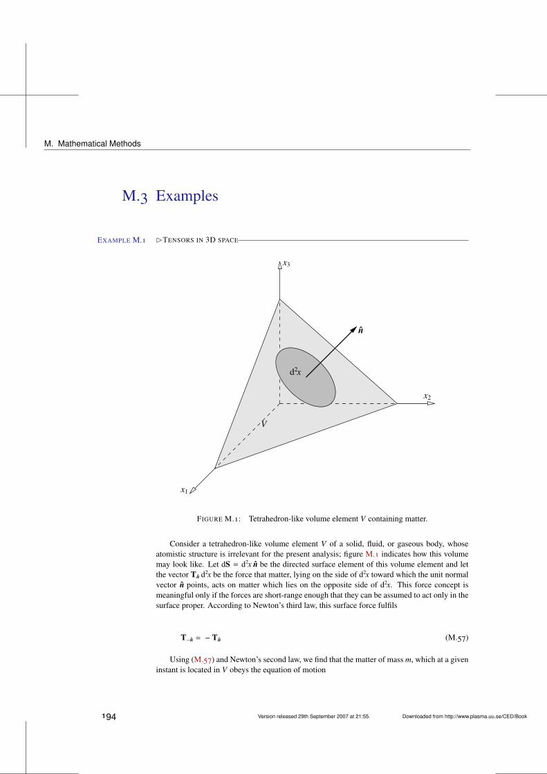
M. Mathematical Methods
M.3 Examples
BTENSORS IN 3D SPACEEXAMPLE M.1
x1
d2x
n
x3
x2
V
FIGURE M.1: Tetrahedron-like volume element V containing matter.
Consider a tetrahedron-like volume element V of a solid, fluid, or gaseous body, whoseatomistic structure is irrelevant for the present analysis; figure M.1 indicates how this volumemay look like. Let dS = d2x n be the directed surface element of this volume element and letthe vector Tn d2x be the force that matter, lying on the side of d2x toward which the unit normalvector n points, acts on matter which lies on the opposite side of d2x. This force concept ismeaningful only if the forces are short-range enough that they can be assumed to act only in thesurface proper. According to Newton’s third law, this surface force fulfils
T−n = − Tn (M.57)
Using (M.57) and Newton’s second law, we find that the matter of mass m, which at a giveninstant is located in V obeys the equation of motion
194 Version released 29th September 2007 at 21:55. Downloaded from http://www.plasma.uu.se/CED/Book
Examples
Tn d2x − cos θ1Tx1 d2x − cos θ2Tx2 d2x − cos θ3Tx3 d2x + Fext = ma (M.58)
where Fext is the external force and a is the acceleration of the volume element. In other words
Tn = n1Tx1 + n2Tx2 + n3Tx3 +md2x
(a −
Fext
m
)(M.59)
Since both a and Fext/m remain finite whereas m/d2x→ 0 as V → 0, one finds that in this limit
Tn =3
∑i=1
niTxi ≡ niTxi (M.60)
From the above derivation it is clear that equation (M.60) above is valid not only in equilibriumbut also when the matter in V is in motion.
Introducing the notation
Ti j =(Txi
)j (M.61)
for the jth component of the vector Txi , we can write equation (M.60) in component form asfollows
T n j = (Tn) j =3
∑i=1
niTi j ≡ niTi j (M.62)
Using equation (M.62) above, we find that the component of the vector Tn in the direction ofan arbitrary unit vector m is
T nm = Tn · m
=3
∑j=1
T n jm j =3
∑j=1
(3
∑i=1
niTi j
)m j ≡ niTi jm j = n · T · m
(M.63)
Hence, the jth component of the vector Txi , here denoted Ti j, can be interpreted as the i jthcomponent of a tensor T. Note that T nm is independent of the particular coordinate system usedin the derivation.
We shall now show how one can use the momentum law (force equation) to derive theequation of motion for an arbitrary element of mass in the body. To this end we consider apart V of the body. If the external force density (force per unit volume) is denoted by f and thevelocity for a mass element dm is denoted by v, we obtain
ddt
∫V
v dm =∫
Vf d3x +
∫S
Tn d2x (M.64)
The jth component of this equation can be written∫V
ddtv j dm =
∫V
f j d3x +∫
ST n j d2x =
∫V
f j d3x +∫
SniTi j d2x (M.65)
where, in the last step, equation (M.62) was used. Setting dm = ρ d3x and using the divergencetheorem on the last term, we can rewrite the result as∫
Vρ
ddtv j d3x =
∫V
f j d3x +∫
V
∂Ti j
∂xid3x (M.66)
Since this formula is valid for any arbitrary volume, we must require that
Downloaded from http://www.plasma.uu.se/CED/Book Version released 29th September 2007 at 21:55. 195
M. Mathematical Methods
ρddtv j − f j −
∂Ti j
∂xi= 0 (M.67)
or, equivalently
ρ∂v j
∂t+ ρv · ∇v j − f j −
∂Ti j
∂xi= 0 (M.68)
Note that ∂v j/∂t is the rate of change with time of the velocity component v j at a fixed pointx = (x1, x1, x3).
C END OF EXAMPLE M.1
BCONTRAVARIANT AND COVARIANT VECTORS IN FLAT LORENTZ SPACEEXAMPLE M.2
The 4D Lorentz space L4 has a simple metric which can be described either by the metrictensor
gµν =
1 if µ = ν = 0−1 if µ = ν = i = j = 1, 2, 30 if µ , ν
(M.69)
which, in matrix notation, is represented as
(gµν) =
1 0 0 00 −1 0 00 0 −1 00 0 0 −1
(M.70)
i.e., a matrix with a main diagonal that has the sign sequence, or signature, +,−,−,− or
gµν =
−1 if µ = ν = 01 if µ = ν = i = j = 1, 2, 30 if µ , ν
(M.71)
which, in matrix notation, is represented as
(gµν) =
−1 0 0 00 1 0 00 0 1 00 0 0 1
(M.72)
i.e., a matrix with signature −,+,+,+.
Consider an arbitrary contravariant four-vector aν in this space. In component form it canbe written:
aνdef≡ (a0, a1, a2, a3) = (a0, a) (M.73)
According to the index lowering rule, equation (M.20) on page 187, we obtain the covariantversion of this vector as
196 Version released 29th September 2007 at 21:55. Downloaded from http://www.plasma.uu.se/CED/Book
Examples
aµdef≡ (a0, a1, a2, a3) = gµνaν (M.74)
In the +,−,−,− metric we obtain
µ = 0 : a0 = 1 · a0 + 0 · a1 + 0 · a2 + 0 · a3 = a0 (M.75)
µ = 1 : a1 = 0 · a0 − 1 · a1 + 0 · a2 + 0 · a3 = −a1 (M.76)
µ = 2 : a2 = 0 · a0 + 0 · a1 − 1 · a2 + 0 · a3 = −a2 (M.77)
µ = 3 : a3 = 0 · a0 + 0 · a1 + 0 · a2 + 1 · a3 = −a3 (M.78)
or
aµ = (a0, a1, a2, a3) = (a0,−a1,−a2,−a3) = (a0,−a) (M.79)
Radius 4-vector itself in L4 and in this metric is given by
xµ = (x0, x1, x2, x3) = (x0, x, y, z) = (x0, x)
xµ = (x0, x1, x2, x3) = (x0,−x1,−x2,−x3) = (x0,−x)(M.80)
where x0 = ct.
Analogously, using the −,+,+,+ metric we obtain
aµ = (a0, a1, a2, a3) = (−a0, a1, a2, a3) = (−a0, a) (M.81)
C END OF EXAMPLE M.2
BINNER PRODUCTS IN COMPLEX VECTOR SPACE EXAMPLE M.3
A 3D complex vector A is a vector in C3 (or, if we like, in R6), expressed in terms of tworeal vectors aR and aI in R3 in the following way
Adef≡ aR + iaI = aR aR + iaI aI
def≡ AA ∈ C3 (M.82)
The inner product of A with itself may be defined as
A2 def≡ A · A = a2
R − a2I + 2iaR · aI
def≡ A2 ∈ C (M.83)
from which we find that
A =√
a2R − a2
I + 2iaR · aI ∈ C (M.84)
Using this in equation (M.82), we see that we can interpret this so that the complex unit vectoris
A =AA=
aR√a2
R − a2I + 2iaR · aI
aR + iaI√
a2R − a2
I + 2iaR · aIaI
=aR
√a2
R − a2I − 2iaR · aI
a2R + a2
IaR + i
aI
√a2
R − a2I − 2iaR · aI
a2R + a2
IaI ∈ C3
(M.85)
Downloaded from http://www.plasma.uu.se/CED/Book Version released 29th September 2007 at 21:55. 197
M. Mathematical Methods
On the other hand, the definition of the scalar product in terms of the inner product of complexvector with its own complex conjugate yields
|A|2def≡ A · A∗ = a2
R + a2I = |A|
2 (M.86)
with the help of which we can define the unit vector as
A =A|A|=
aR√a2
R + a2I
aR + iaI√
a2R + a2
I
aI
=aR
√a2
R + a2I
a2R + a2
IaR + i
aI
√a2
R + a2I
a2R + a2
IaI ∈ C3
(M.87)
C END OF EXAMPLE M.3
BSCALAR PRODUCT, NORM AND METRIC IN LORENTZ SPACEEXAMPLE M.4
In L4 the metric tensor attains a simple form [see example M.2 on page 196] and, hence,the scalar product in equation (M.28) on page 188 can be evaluated almost trivially. For the+,−,−,− signature it becomes
aµbµ = (a0,−a) · (b0,b) = a0b0 − a · b (M.88)
The important scalar product of the L4 radius four-vector with itself becomes
xµxµ = (x0,−x) · (x0, x) = (ct,−x) · (ct, x)
= (ct)2 − (x1)2 − (x2)2 − (x3)2 = s2 (M.89)
which is the indefinite, real norm of L4. The L4 metric is the quadratic differential form
ds2 = dxµdxµ = c2(dt)2 − (dx1)2 − (dx2)2 − (dx3)2 (M.90)
C END OF EXAMPLE M.4
198 Version released 29th September 2007 at 21:55. Downloaded from http://www.plasma.uu.se/CED/Book
Examples
BTHE FOUR-DEL OPERATOR IN LORENTZ SPACE EXAMPLE M.5
In L4 the contravariant form of the four-del operator can be represented as
∂µ =
(1c∂
∂t,−∂
)=
(1c∂
∂t,−∇
)(M.91)
and the covariant form as
∂µ =
(1c∂
∂t,∂
)=
(1c∂
∂t,∇
)(M.92)
Taking the scalar product of these two, one obtains
∂µ∂µ =1c2
∂2
∂t2 − ∇2 = 2 (M.93)
which is the d’Alembert operator, sometimes denoted , and sometimes defined with an oppo-site sign convention.
C END OF EXAMPLE M.5
BGRADIENTS OF SCALAR FUNCTIONS OF RELATIVE DISTANCES IN 3D EXAMPLE M.6
Very often electrodynamic quantities are dependent on the relative distance in R3 betweentwo vectors x and x′, i.e., on |x − x′|. In analogy with equation (M.35) on page 190, we candefine the primed del operator in the following way:
∇′ = xi
∂
∂x′i= ∂′ (M.94)
Using this, the unprimed version, equation (M.35) on page 190, and elementary rules of differ-entiation, we obtain the following two very useful results:
∇ (|x − x′|) = xi∂|x − x′|∂xi
=x − x′
|x − x′|= − xi
∂|x − x′|∂x′i
= − ∇′ (|x − x′|)(M.95)
and
∇
(1
|x − x′|
)= −
x − x′
|x − x′|3= − ∇′
(1
|x − x′|
)(M.96)
C END OF EXAMPLE M.6
Downloaded from http://www.plasma.uu.se/CED/Book Version released 29th September 2007 at 21:55. 199
M. Mathematical Methods
BDIVERGENCE IN 3DEXAMPLE M.7
For an arbitrary R3 vector field a(x′), the following relation holds:
∇′ ·
(a(x′)|x − x′|
)=∇′ · a(x′)|x − x′|
+ a(x′) · ∇′(
1|x − x′|
)(M.97)
which demonstrates how the primed divergence, defined in terms of the primed del operator inequation (M.94) on page 199, works.
C END OF EXAMPLE M.7
BTHE LAPLACIAN AND THE DIRAC DELTAEXAMPLE M.8
A very useful formula in 3D R3 is
∇ · ∇
(1
|x − x′|
)= ∇2
(1
|x − x′|
)= − 4πδ(x − x′) (M.98)
where δ(x − x′) is the 3D Dirac delta ‘function’. This formula follows directly from the factthat ∫
Vd3x∇ · ∇
(1
|x − x′|
)=
∫V
d3x∇ ·(−
x − x′
|x − x′|3
)=
∮Sd2x n ·
(−
x − x′
|x − x′|3
)(M.99)
equals −4π if the integration volume V(S ), enclosed by the surface S (V), includes x = x′, andequals 0 otherwise.
C END OF EXAMPLE M.8
BTHE CURL OF A GRADIENTEXAMPLE M.9
Using the definition of the R3 curl, equation (M.46) on page 192, and the gradient, equa-tion (M.41) on page 191, we see that
∇ × [∇α(x)] = εi jk xi∂ j∂kα(x) (M.100)
which, due to the assumed well-behavedness of α(x), vanishes:
εi jk xi∂ j∂kα(x) = εi jk∂
∂x j
∂
∂xkα(x)xi
=
(∂2
∂x2∂x3−
∂2
∂x3∂x2
)α(x)x1
+
(∂2
∂x3∂x1−
∂2
∂x1∂x3
)α(x)x2
+
(∂2
∂x1∂x2−
∂2
∂x2∂x1
)α(x)x3
≡ 0
(M.101)
200 Version released 29th September 2007 at 21:55. Downloaded from http://www.plasma.uu.se/CED/Book
Examples
We thus find that
∇ × [∇α(x)] ≡ 0 (M.102)
for any arbitrary, well-behaved R3 scalar field α(x).
In 4D we note that for any well-behaved four-scalar field α(xκ)
(∂µ∂ν − ∂ν∂µ)α(xκ) ≡ 0 (M.103)
so that the four-curl of a four-gradient vanishes just as does a curl of a gradient in R3.
Hence, a gradient is always irrotational.
C END OF EXAMPLE M.9
BTHE DIVERGENCE OF A CURL EXAMPLE M.10
With the use of the definitions of the divergence (M.43) and the curl, equation (M.46) onpage 192, we find that
∇ · [∇ × a(x)] = ∂i[∇ × a(x)]i = εi jk∂i∂ jak(x) (M.104)
Using the definition for the Levi-Civita symbol, defined by equation (M.18) on page 187, wefind that, due to the assumed well-behavedness of a(x),
∂iεi jk∂ jak(x) =∂
∂xiεi jk
∂
∂x jak
=
(∂2
∂x2∂x3−
∂2
∂x3∂x2
)a1(x)
+
(∂2
∂x3∂x1−
∂2
∂x1∂x3
)a2(x)
+
(∂2
∂x1∂x2−
∂2
∂x2∂x1
)a3(x)
≡ 0
(M.105)
i.e., that
∇ · [∇ × a(x)] ≡ 0 (M.106)
for any arbitrary, well-behaved R3 vector field a(x).
In 4D, the four-divergence of the four-curl is not zero, for
∂νGµν = ∂µ∂νaν(xκ) −2aµ(xκ) , 0 (M.107)
C END OF EXAMPLE M.10
Downloaded from http://www.plasma.uu.se/CED/Book Version released 29th September 2007 at 21:55. 201
M. Mathematical Methods
M.4 Bibliography[1] G. B. ARFKEN AND H. J. WEBER, Mathematical Methods for Physicists, fourth, interna-
tional ed., Academic Press, Inc., San Diego, CA . . . , 1995, ISBN 0-12-059816-7.
[2] R. A. DEAN, Elements of Abstract Algebra, John Wiley & Sons, Inc., New York, NY . . . ,1967, ISBN 0-471-20452-8.
[3] A. A. EVETT, Permutation symbol approach to elementary vector analysis, American Jour-nal of Physics, 34 (1965), pp. 503–507.
[4] P. M. MORSE AND H. FESHBACH, Methods of Theoretical Physics, Part I. McGraw-HillBook Company, Inc., New York, NY . . . , 1953, ISBN 07-043316-8.
[5] B. SPAIN, Tensor Calculus, third ed., Oliver and Boyd, Ltd., Edinburgh and London, 1965,ISBN 05-001331-9.
[6] W. E. THIRRING, Classical Mathematical Physics, Springer-Verlag, New York, Vienna,1997, ISBN 0-387-94843-0.
202 Version released 29th September 2007 at 21:55. Downloaded from http://www.plasma.uu.se/CED/Book
Downloaded from http://www.plasma.uu.se/CED/Book Version released 29th September 2007 at 21:55.
Index
acceleration field, 104advanced time, 50Ampère’s law, 6Ampère-turn density, 61anisotropic, 120anomalous dispersion, 121antenna, 81antenna current, 81antenna feed point, 82antisymmetric tensor, 151associated Legendre polynomial, 91associative, 142axial gauge, 53axial vector, 151, 189
Bessel functions, 88Biot-Savart’s law, 8birefringent, 120braking radiation, 111bremsstrahlung, 111, 117
canonically conjugate four-momentum, 160canonically conjugate momentum, 160, 192canonically conjugate momentum density,
167Cerenkov radiation, 122characteristic impedance, 31classical electrodynamics, 1, 9closed algebraic structure, 142coherent radiation, 116collisional interaction, 120complete α-Lorenz gauge, 52complex field six-vector, 24complex notation, 35complex vector, 197component notation, 184concentration, 191conservative field, 12conservative forces, 164
constitutive relations, 15contravariant component form, 138, 184contravariant field tensor, 151contravariant four-tensor field, 187contravariant four-vector, 186contravariant four-vector field, 141contravariant vector, 138convection potential, 131convective derivative, 13cosine integral, 85Coulomb gauge, 51Coulomb’s law, 2covariant, 136covariant component form, 184covariant field tensor, 152covariant four-tensor field, 187covariant four-vector, 186covariant four-vector field, 141covariant vector, 138cross product, 189curl, 191cutoff, 133cyclotron radiation, 113, 117
d’Alembert operator, 28, 47, 147, 198del operator, 190del squared, 191differential distance, 140differential vector operator, 190dipole antennas, 81Dirac delta, 200Dirac’s symmetrised Maxwell equations, 16dispersive, 121displacement current, 11divergence, 191dot product, 188dual electromagnetic tensor, 153dual vector, 138duality transformation, 17, 153
203
Index
dummy index, 138dyadic product, 188dyons, 17
E1 radiation, 94E2 radiation, 97Einstein’s summation convention, 184electric charge conservation law, 10electric charge density, 4electric conductivity, 11electric current density, 8electric dipole moment, 93electric dipole moment vector, 58electric dipole radiation, 94electric displacement, 15electric displacement current, 22electric displacement vector, 57, 59electric field, 3electric field energy, 63electric monopole moment, 57electric permittivity, 120electric polarisation, 58electric quadrupole moment tensor, 58electric quadrupole radiation, 97electric quadrupole tensor, 96electric susceptibility, 59electric volume force, 64electricity, 2electrodynamic potentials, 44electromagnetic field tensor, 151electromagnetic scalar potential, 45electromagnetic vector potential, 44electromagnetism, 1electromagnetodynamic equations, 16electromagnetodynamics, 17electromotive force (EMF), 12electrostatic scalar potential, 43electrostatics, 2electroweak theory, 1energy theorem in Maxwell’s theory, 63equation of continuity, 10, 148equations of classical electrostatics, 9equations of classical magnetostatics, 9Euclidean space, 143Euclidean vector space, 139Euler-Lagrange equation, 166Euler-Lagrange equations, 167, 192
Euler-Mascheroni constant, 85event, 142
far field, 72far zone, 75Faraday’s law, 12field, 185field Lagrange density, 168field point, 4field quantum, 133fine structure constant, 118, 133four-current, 147four-del operator, 190four-dimensional Hamilton equations, 160four-dimensional vector space, 138four-divergence, 191four-gradient, 191four-Hamiltonian, 160four-Lagrangian, 158four-momentum, 146four-potential, 147four-scalar, 185four-tensor fields, 187four-vector, 141, 185four-velocity, 145Fourier integral, 30Fourier series, 29Fourier transform, 30, 48free-free radiation, 111functional derivative, 166fundamental tensor, 138, 184, 187
Galileo’s law, 135gauge fixing, 53gauge function, 46gauge invariant, 46gauge transformation, 46Gauss’s law of electrostatics, 5general inhomogeneous wave equations, 46generalised coordinate, 160, 192generalised four-coordinate, 160Gibbs’ notation, 190gradient, 191Green function, 48, 91group theory, 142group velocity, 121
Hamilton density, 167
204 Version released 29th September 2007 at 21:55. Downloaded from http://www.plasma.uu.se/CED/Book
Hamilton density equations, 167Hamilton equations, 160, 193Hamilton function, 193Hamilton gauge, 53Hamiltonian, 193Heaviside potential, 131Heaviside-Larmor-Rainich transformation,
17Helmholtz’ theorem, 47help vector, 90Hertz’ method, 89Hertz’ vector, 90Hodge star operator, 17homogeneous wave equation, 28Hooke’s law, 164Huygen’s principle, 48
identity element, 142in a medium, 123incoherent radiation, 116indefinite norm, 139index contraction, 138index lowering, 138induction field, 72inertial reference frame, 135inertial system, 135inhomogeneous Helmholtz equation, 48inhomogeneous time-independent wave equa-
tion, 48inhomogeneous wave equation, 47inner product, 188instantaneous, 108interaction Lagrange density, 168intermediate field, 75invariant, 185invariant line element, 140inverse element, 142inverse Fourier transform, 30irrotational, 6, 192
Jacobi identity, 154
Kelvin function, 118kinetic energy, 164, 192kinetic momentum, 163Kronecker delta, 186
Lagrange density, 165
Lagrange function, 164, 192Lagrangian, 164, 192Laplace operator, 191Laplacian, 191Larmor formula for radiated power, 108law of inertia, 135Legendre polynomial, 91Legendre transformation, 193Levi-Civita tensor, 187Liénard-Wiechert potentials, 99, 130, 150light cone, 141light-like interval, 141line element, 188linear mass density, 165longitudinal component, 32loop antenna, 85Lorentz boost parameter, 145Lorentz force, 14, 63, 130Lorentz space, 139, 184Lorentz transformation, 130, 137Lorenz-Lorentz gauge, 51Lorenz-Lorentz gauge condition, 47, 148lowering of index, 187
M1 radiation, 96Møller scattering, 119Mach cone, 124macroscopic Maxwell equations, 120magnetic charge density, 16magnetic current density, 16magnetic dipole moment, 60, 96magnetic dipole radiation, 96magnetic displacement current, 22magnetic field, 7magnetic field energy, 63magnetic field intensity, 61magnetic flux, 12magnetic flux density, 8magnetic four-current, 154magnetic induction, 8magnetic monopole equation of continuity,
17magnetic monopoles, 16magnetic permeability, 120magnetic susceptibility, 61magnetisation, 61magnetisation currents, 60
Downloaded from http://www.plasma.uu.se/CED/Book Version released 29th September 2007 at 21:55. 205
Index
magnetising field, 15, 57, 61magnetostatic vector potential, 44magnetostatics, 6massive photons, 171mathematical group, 142matrix form, 186Maxwell stress tensor, 65Maxwell’s macroscopic equations, 16, 62Maxwell’s microscopic equations, 15Maxwell-Lorentz equations, 15mechanical Lagrange density, 168metric, 184, 188metric tensor, 138, 184, 187Minkowski equation, 160Minkowski space, 143mixed four-tensor field, 187mixing angle, 17momentum theorem in Maxwell’s theory,
65monochromatic, 69multipole expansion, 89, 92
near zone, 75Newton’s first law, 135Newton-Lorentz force equation, 160non-Euclidean space, 139non-linear effects, 11norm, 138, 198null vector, 141
observation point, 4Ohm’s law, 11one-dimensional wave equation, 33outer product, 188
Parseval’s identity, 79, 118, 132phase velocity, 120photon, 133physical measurable, 35plane wave, 33plasma, 121plasma frequency, 122Poincaré gauge, 53Poisson equation, 130Poisson’s equation, 43polar vector, 151, 189polarisation charges, 59polarisation currents, 60
polarisation potential, 90polarisation vector, 89positive definite, 143positive definite norm, 139potential energy, 164, 192potential theory, 91power flux, 63Poynting vector, 63Poynting’s theorem, 63Proca Lagrangian, 170propagator, 48proper time, 141pseudo-Riemannian space, 143pseudoscalar, 183pseudoscalars, 190pseudotensor, 183pseudotensors, 190pseudovector, 151, 183, 189
quadratic differential form, 140, 188quantum chromodynamics, 1quantum electrodynamics, 1, 51quantum mechanical nonlinearity, 4
radial gauge, 53radiation field, 72, 75, 104radiation fields, 75radiation resistance, 85radius four-vector, 138radius vector, 183raising of index, 187rank, 186rapidity, 145refractive index, 120relative electric permittivity, 65relative magnetic permeability, 65relative permeability, 120relative permittivity, 120Relativity principle, 136relaxation time, 30rest mass density, 168retarded Coulomb field, 75retarded potentials, 50retarded relative distance, 99retarded time, 50Riemann-Silberstein vector, 24Riemannian metric, 140
206 Version released 29th September 2007 at 21:55. Downloaded from http://www.plasma.uu.se/CED/Book
Riemannian space, 138, 184row vector, 183
scalar, 183, 191scalar field, 142, 185scalar product, 188shock front, 124signature, 139, 196simultaneous coordinate, 128skew-symmetric, 151skin depth, 35source point, 4space components, 139space-like interval, 141space-time, 139special theory of relativity, 135spherical Bessel function of the first kind,
91spherical Hankel function of the first kind,
91spherical waves, 78standard configuration, 136standing wave, 82super-potential, 90synchrotron radiation, 113, 117synchrotron radiation lobe width, 114
telegrapher’s equation, 33, 120temporal dispersive media, 11temporal gauge, 53tensor, 183tensor contraction, 188tensor field, 186tensor notation, 187tensor product, 189three-dimensional functional derivative, 167time component, 139time-dependent Poisson’s equation, 51time-harmonic wave, 29time-independent diffusion equation, 31time-independent telegrapher’s equation, 33time-independent wave equation, 31time-like interval, 141total charge, 57transverse components, 32transverse gauge, 52
uncoupled inhomogeneous wave equations,47
vacuum permeability, 6vacuum permittivity, 2vacuum polarisation effects, 4vacuum wave number, 31variational principle, 192Vavilov-Cerenkov cone, 124Vavilov-Cerenkov radiation, 122, 124vector, 183vector product, 189velocity field, 104velocity gauge condition, 52virtual simultaneous coordinate, 100, 104
wave equations, 27wave vector, 33, 121world line, 142
Young’s modulus, 165Yukawa meson field, 170
Downloaded from http://www.plasma.uu.se/CED/Book Version released 29th September 2007 at 21:55. 207