Electromagnetic Field Theory - Sicyon · Electromagnetic Field Theory BO THIDÉ Swedish Institute...
221
Electromagnetic Field Theory B O T HIDÉ ϒ UPSILON B OOKS
-
Upload
nguyenkiet -
Category
Documents
-
view
256 -
download
3
Transcript of Electromagnetic Field Theory - Sicyon · Electromagnetic Field Theory BO THIDÉ Swedish Institute...
ElectromagneticField Theory
BO THIDÉ
ϒUPSILON BOOKS

ELECTROMAGNETIC FIELD THEORY

ElectromagneticField Theory
BO THIDÉ
Swedish Institute of Space PhysicsUppsala, Sweden
and
Department of Astronomy and Space PhysicsUppsala University, Sweden
and
LOIS Space CentreSchool of Mathematics and Systems Engineering
Växjö University, Sweden
ϒUPSILON BOOKS · UPPSALA · SWEDEN
Also available
ELECTROMAGNETIC FIELD THEORY
EXERCISES
by
Tobia Carozzi, Anders Eriksson, Bengt Lundborg,Bo Thidé and Mattias Waldenvik
Freely downloadable fromwww.plasma.uu.se/CED
This book was typeset in LATEX 2ε (based on TEX 3.141592 and Web2C7.4.4) on an HP Visu-alize9000⁄3600 workstation running HP-UX11.11.
Copyright©1997–2006 byBo ThidéUppsala, SwedenAll rights reserved.
Electromagnetic Field TheoryISBN X-XXX-XXXXX-X
To the memory of professorLEV M IKHAILOVICH ERUKHIMOV (1936–1997)
dear friend, great physicist, poetand a truly remarkable man.

Downloaded from http://www.plasma.uu.se/CED/Book Version released 23rd December 2007 at 00:02.
CONTENTS
Contents ix
List of Figures xiii
Preface xv
1 Classical Electrodynamics 1
1.1 Electrostatics 2
1.1.1 Coulomb’s law 2
1.1.2 The electrostatic field 3
1.2 Magnetostatics 6
1.2.1 Ampère’s law 6
1.2.2 The magnetostatic field 7
1.3 Electrodynamics 9
1.3.1 Equation of continuity for electric charge 10
1.3.2 Maxwell’s displacement current 10
1.3.3 Electromotive force 11
1.3.4 Faraday’s law of induction 12
1.3.5 Maxwell’s microscopic equations 15
1.3.6 Maxwell’s macroscopic equations 15
1.4 Electromagnetic duality 16
1.5 Bibliography 18
1.6 Examples 20
2 Electromagnetic Waves 25
2.1 The wave equations 26
2.1.1 The wave equation forE 26
2.1.2 The wave equation forB 27
2.1.3 The time-independent wave equation forE 27
ix
Contents
2.2 Plane waves 30
2.2.1 Telegrapher’s equation 31
2.2.2 Waves in conductive media 32
2.3 Observables and averages 33
2.4 Bibliography 34
2.5 Example 36
3 Electromagnetic Potentials 39
3.1 The electrostatic scalar potential 39
3.2 The magnetostatic vector potential 40
3.3 The electrodynamic potentials 40
3.4 Gauge transformations 41
3.5 Gauge conditions 42
3.5.1 Lorenz-Lorentz gauge 43
3.5.2 Coulomb gauge 47
3.5.3 Velocity gauge 49
3.6 Bibliography 49
3.7 Examples 51
4 Electromagnetic Fields and Matter 53
4.1 Electric polarisation and displacement 53
4.1.1 Electric multipole moments 53
4.2 Magnetisation and the magnetising field 56
4.3 Energy and momentum 58
4.3.1 The energy theorem in Maxwell’s theory 58
4.3.2 The momentum theorem in Maxwell’s theory 59
4.4 Bibliography 62
4.5 Example 63
5 Electromagnetic Fields from Arbitrary Source Distributions 65
5.1 The magnetic field 67
5.2 The electric field 69
5.3 The radiation fields 71
5.4 Radiated energy 74
5.4.1 Monochromatic signals 74
5.4.2 Finite bandwidth signals 75
5.5 Bibliography 76
6 Electromagnetic Radiation and Radiating Systems 77
6.1 Radiation from an extended source volume at rest 77
6.1.1 Radiation from a one-dimensional current distribution 78
x Version released 23rd December 2007 at 00:02. Downloaded from http://www.plasma.uu.se/CED/Book
6.1.2 Radiation from a two-dimensional current distribution 81
6.2 Radiation from a localised source volume at rest 85
6.2.1 The Hertz potential 85
6.2.2 Electric dipole radiation 90
6.2.3 Magnetic dipole radiation 91
6.2.4 Electric quadrupole radiation 93
6.3 Radiation from a localised charge in arbitrary motion 93
6.3.1 The Liénard-Wiechert potentials 94
6.3.2 Radiation from an accelerated point charge 97
6.3.3 Bremsstrahlung 105
6.3.4 Cyclotron and synchrotron radiation (magnetic bremsstrahlung)1086.3.5 Radiation from charges moving in matter 116
6.4 Bibliography 123
6.5 Examples 124
7 Relativistic Electrodynamics 131
7.1 The special theory of relativity 131
7.1.1 The Lorentz transformation 132
7.1.2 Lorentz space 134
7.1.3 Minkowski space 139
7.2 Covariant classical mechanics 141
7.3 Covariant classical electrodynamics 143
7.3.1 The four-potential 143
7.3.2 The Liénard-Wiechert potentials 144
7.3.3 The electromagnetic field tensor 146
7.4 Bibliography 150
8 Electromagnetic Fields and Particles 153
8.1 Charged particles in an electromagnetic field 153
8.1.1 Covariant equations of motion 153
8.2 Covariant field theory 159
8.2.1 Lagrange-Hamilton formalism for fields and interactions1608.3 Bibliography 167
8.4 Example 169
F Formulæ 171
F.1 The electromagnetic field 171
F.1.1 Maxwell’s equations 171
F.1.2 Fields and potentials 172
F.1.3 Force and energy 172
F.2 Electromagnetic radiation 172
Downloaded from http://www.plasma.uu.se/CED/Book Version released 23rd December 2007 at 00:02. xi
Contents
F.2.1 Relationship between the field vectors in a plane wave172F.2.2 The far fields from an extended source distribution 172
F.2.3 The far fields from an electric dipole 173
F.2.4 The far fields from a magnetic dipole 173
F.2.5 The far fields from an electric quadrupole 173
F.2.6 The fields from a point charge in arbitrary motion 173
F.3 Special relativity 174
F.3.1 Metric tensor 174
F.3.2 Covariant and contravariant four-vectors 174
F.3.3 Lorentz transformation of a four-vector 174
F.3.4 Invariant line element 174
F.3.5 Four-velocity 174
F.3.6 Four-momentum 175
F.3.7 Four-current density 175
F.3.8 Four-potential 175
F.3.9 Field tensor 175
F.4 Vector relations 175
F.4.1 Spherical polar coordinates 176
F.4.2 Vector formulae 176
F.5 Bibliography 178
M Mathematical Methods 179
M.1 Scalars, vectors and tensors 179
M.1.1 Vectors 180
M.1.2 Fields 181
M.1.3 Vector algebra 185
M.1.4 Vector analysis 187
M.2 Analytical mechanics 189
M.2.1 Lagrange’s equations 189
M.2.2 Hamilton’s equations 190
M.3 Examples 192
M.4 Bibliography 200
Index 201
xii Version released 23rd December 2007 at 00:02. Downloaded from http://www.plasma.uu.se/CED/Book
Downloaded from http://www.plasma.uu.se/CED/Book Version released 23rd December 2007 at 00:02.
L IST OF FIGURES
1.1 Coulomb interaction between two electric charges 3
1.2 Coulomb interaction for a distribution of electric charges 5
1.3 Ampère interaction 7
1.4 Moving loop in a varyingB field 13
5.1 Radiation in the far zone 73
6.1 Linear antenna 79
6.2 Electric dipole antenna geometry 80
6.3 Loop antenna 82
6.4 Multipole radiation geometry 87
6.5 Electric dipole geometry 89
6.6 Radiation from a moving charge in vacuum 94
6.7 An accelerated charge in vacuum 96
6.8 Angular distribution of radiation during bremsstrahlung 105
6.9 Location of radiation during bremsstrahlung 107
6.10 Radiation from a charge in circular motion 109
6.11 Synchrotron radiation lobe width 111
6.12 The perpendicular electric field of a moving charge 114
6.13 Electron-electron scattering 116
6.14 Vavilov-Cerenkov cone 120
7.1 Relative motion of two inertial systems 133
7.2 Rotation in a 2D Euclidean space 139
7.3 Minkowski diagram 140
8.1 Linear one-dimensional mass chain 160
M.1 Tetrahedron-like volume element of matter 192
xiii

Downloaded from http://www.plasma.uu.se/CED/Book Version released 23rd December 2007 at 00:02.
PREFACE
This book is the result of a more than thirty year long love affair. In 1972, I tookmy first advanced course in electrodynamics at the Department of TheoreticalPhysics, Uppsala University. A year later, I joined the research group there andtook on the task of helping professorPER OLOF FRÖMAN, who later become myPh.D. thesis advisor, with the preparation of a new version of his lecture notes onthe Theory of Electricity. These two things opened up my eyesfor the beauty andintricacy of electrodynamics, already at the classical level, and I fell in love withit. Ever since that time, I have on and off had reason to return to electrodynamics,both in my studies, research and the teaching of a course in advanced electrody-namics at Uppsala University some twenty odd years after I experienced the firstencounter with this subject.
The current version of the book is an outgrowth of the lecturenotes that I pre-pared for the four-credit course Electrodynamics that was introduced in the Up-psala University curriculum in1992, to become the five-credit course ClassicalElectrodynamics in1997. To some extent, parts of these notes were based on lec-ture notes prepared, in Swedish, by my friend and colleagueBENGT LUNDBORG,who created, developed and taught the earlier, two-credit course ElectromagneticRadiation at our faculty.
Intended primarily as a textbook for physics students at theadvanced under-graduate or beginning graduate level, it is hoped that the present book may beuseful for research workers too. It provides a thorough treatment of the theoryof electrodynamics, mainly from a classical field theoretical point of view, andincludes such things as formal electrostatics and magnetostatics and their uni-fication into electrodynamics, the electromagnetic potentials, gauge transforma-tions, covariant formulation of classical electrodynamics, force, momentum andenergy of the electromagnetic field, radiation and scattering phenomena, electro-magnetic waves and their propagation in vacuum and in media,and covariantLagrangian/Hamiltonian field theoretical methods for electromagneticfields, par-ticles and interactions. The aim has been to write a book thatcan serve both asan advanced text in Classical Electrodynamics and as a preparation for studies inQuantum Electrodynamics and related subjects.
In an attempt to encourage participation by other scientists and students inthe authoring of this book, and to ensure its quality and scope to make it useful
xv
Preface
in higher university education anywhere in the world, it wasproduced within aWorld-Wide Web (WWW) project. This turned out to be a rather successful move.By making an electronic version of the book freely down-loadable on the net,comments have been received from fellow Internet physicists around the worldand from WWW ‘hit’ statistics it seems that the book serves asa frequently usedInternet resource.1 This way it is hoped that it will be particularly useful forstudents and researchers working under financial or other circumstances that makeit difficult to procure a printed copy of the book.
Thanks are due not only to Bengt Lundborg for providing the inspiration towrite this book, but also to professorCHRISTERWAHLBERG and professorGÖRAN
FÄLDT , Uppsala University, and professorYAKOV ISTOMIN, Lebedev Institute,Moscow, for interesting discussions on electrodynamics andrelativity in generaland on this book in particular. Comments from former graduate studentsMATTIAS
WALDENVIK , TOBIA CAROZZI andROGERKARLSSONas well asANDERSERIKS-SON, all at the Swedish Institute of Space Physics in Uppsala andwho all haveparticipated in the teaching on the material covered in the course and in this bookare gratefully acknowledged. Thanks are also due to my long-term space physicscolleagueHELMUT KOPKA of the Max-Planck-Institut für Aeronomie, Lindau,Germany, who not only taught me about the practical aspects of high-power radiowave transmitters and transmission lines, but also about the more delicate aspectsof typesetting a book in TEX and LATEX. I am particularly indebted to AcademicianprofessorV ITALIY LAZAREVICH GINZBURG, 2003 Nobel Laureate in Physics, forhis many fascinating and very elucidating lectures, comments and historical noteson electromagnetic radiation and cosmic electrodynamics while cruising on theVolga river at our joint Russian-Swedish summer schools during the1990s, andfor numerous private discussions over the years.
Finally, I would like to thank all students and Internet users who have down-loaded and commented on the book during its life on the World-Wide Web.
I dedicate this book to my sonMATTIAS, my daughterKAROLINA , myhigh-school physics teacher,STAFFAN RÖSBY, and to my fellow members of theCAPELLA PEDAGOGICA UPSALIENSIS.
Uppsala, Sweden BO THIDÉ
December,2006 www.physics.irfu.se/∼bt
1At the time of publication of this edition, more than 500 000 downloads have been recorded.
xvi Version released 23rd December 2007 at 00:02. Downloaded from http://www.plasma.uu.se/CED/Book
Downloaded from http://www.plasma.uu.se/CED/Book Version released 23rd December 2007 at 00:02.
1CLASSICAL ELECTRODYNAMICS
Classical electrodynamics deals with electric and magnetic fields and interactionscaused bymacroscopicdistributions of electric charges and currents. This meansthat the concepts of localised electric charges and currents assume the validity ofcertain mathematical limiting processes in which it is considered possible for thecharge and current distributions to be localised in infinitesimally small volumes ofspace. Clearly, this is in contradiction to electromagnetism on a trulymicroscopicscale, where charges and currents have to be treated as spatially extended objectsand quantum corrections must be included. However, the limiting processes usedwill yield results which are correct on small as well as largemacroscopicscales.
It took the genius ofJAMES CLERK MAXWELL to consistently unify electricityand magnetism into a super-theory,electromagnetismor classical electrodynam-ics (CED), and to realise that optics is a subfield of this super-theory. Early inthe20th century,HENDRIK ANTOON LORENTZ took the electrodynamics theoryfurther to the microscopic scale and also laid the foundation for the special the-ory of relativity, formulated byALBERT EINSTEIN in 1905. In the1930s PAUL
A. M. D IRAC expanded electrodynamics to a more symmetric form, includingmagnetic as well as electric charges. With his relativisticquantum mechanics,he also paved the way for the development ofquantum electrodynamics(QED)for which RICHARD P. FEYNMAN , JULIAN SCHWINGER, andSIN-ITIRO TOMON-AGA in 1965 received their Nobel prizes in physics. Around the same time, physi-cists such asSHELDON GLASHOW, ABDUS SALAM , andSTEVEN WEINBERGwereable to unify electrodynamics the weak interaction theory to yet another super-theory,electroweak theory, an achievement which rendered them the Nobel prizein physics 1979. The modern theory of strong interactions,quantum chromody-namics(QCD), is influenced by QED.
In this chapter we start with the force interactions in classical electrostatics
1
1. Classical Electrodynamics
and classical magnetostatics and introduce the static electric and magnetic fieldsto find two uncoupled systems of equations for them. Then we see how the con-servation of electric charge and its relation to electric current leads to the dynamicconnection between electricity and magnetism and how the two can be unifiedinto one ‘super-theory’, classical electrodynamics, described by one system ofeight coupled dynamic field equations—the Maxwell equations.
At the end of this chapter we study Dirac’s symmetrised form of Maxwell’sequations by introducing (hypothetical) magnetic chargesand magnetic currentsinto the theory. While not identified unambiguously in experiments yet, mag-netic charges and currents make the theory much more appealing, for instance byallowing for duality transformations in a most natural way.
1.1 ElectrostaticsThe theory which describes physical phenomena related to the interaction be-tween stationary electric charges or charge distributionsin a finite space whichhas stationary boundaries is calledelectrostatics. For a long time, electrostatics,under the nameelectricity, was considered an independent physical theory of itsown, alongside other physical theories such as magnetism, mechanics, optics andthermodynamics.1
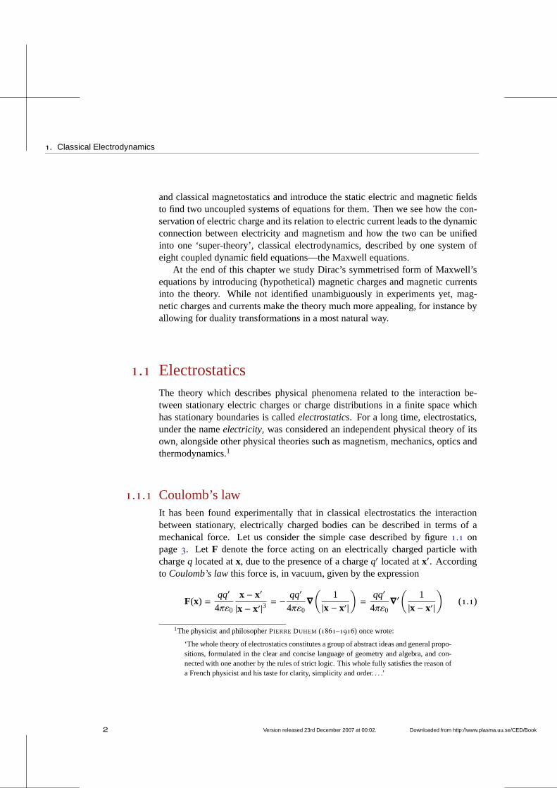
1.1.1 Coulomb’s lawIt has been found experimentally that in classical electrostatics the interactionbetween stationary, electrically charged bodies can be described in terms of amechanical force. Let us consider the simple case describedby figure 1.1 onpage3. Let F denote the force acting on an electrically charged particlewithchargeq located atx, due to the presence of a chargeq′ located atx′. Accordingto Coulomb’s lawthis force is, in vacuum, given by the expression
F(x) =qq′
4πε0
x − x′
|x − x′|3= − qq′
4πε0∇
(1
|x − x′|
)
=qq′
4πε0∇′(
1|x − x′|
)
(1.1)
1The physicist and philosopherPIERRE DUHEM (1861–1916) once wrote:
‘The whole theory of electrostatics constitutes a group of abstract ideas and general propo-sitions, formulated in the clear and concise language of geometry and algebra, and con-nected with one another by the rules of strict logic. This whole fully satisfies the reason ofa French physicist and his taste for clarity, simplicity andorder. . . .’
2 Version released 23rd December 2007 at 00:02. Downloaded from http://www.plasma.uu.se/CED/Book
Electrostatics
q′
q
O
x′
x − x′
x
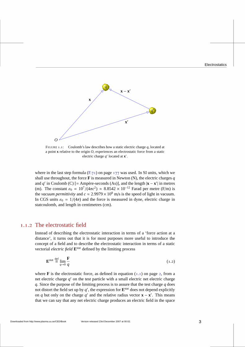
FIGURE1.1: Coulomb’s law describes how a static electric chargeq, located ata pointx relative to the originO, experiences an electrostatic force from a static
electric chargeq′ located atx′.
where in the last step formula (F.71) on page177 was used. In SI units, which weshall use throughout, the forceF is measured in Newton (N), the electric chargesqandq′ in Coulomb (C) [= Ampère-seconds (As)], and the length|x − x′| in metres(m). The constantε0 = 107/(4πc2) ≈ 8.8542× 10⁻¹² Farad per metre (F/m) isthevacuum permittivityandc ≈ 2.9979× 10⁸ m/s is the speed of light in vacuum.In CGS unitsε0 = 1/(4π) and the force is measured in dyne, electric charge instatcoulomb, and length in centimetres (cm).
1.1.2 The electrostatic fieldInstead of describing the electrostatic interaction in terms of a ‘force action at adistance’, it turns out that it is for most purposes more useful to introduce theconcept of a field and to describe the electrostatic interaction in terms of a staticvectorialelectric fieldEstat defined by the limiting process
Estat def≡ limq→0
Fq
(1.2)
whereF is the electrostatic force, as defined in equation (1.1) on page2, from anet electric chargeq′ on the test particle with a small electric net electric chargeq. Since the purpose of the limiting process is to assure that the test chargeq doesnot distort the field set up byq′, the expression forEstat does not depend explicitlyon q but only on the chargeq′ and the relative radius vectorx − x′. This meansthat we can say that any net electric charge produces an electric field in the space
Downloaded from http://www.plasma.uu.se/CED/Book Version released 23rd December 2007 at 00:02. 3
1. Classical Electrodynamics
that surrounds it, regardless of the existence of a second charge anywhere in thisspace.2
Using (1.1) and equation (1.2) on page3, and formula (F.70) on page177,we find that the electrostatic fieldEstat at thefield point x (also known as theobservation point), due to a field-producing electric chargeq′ at thesource pointx′, is given by
Estat(x) =q′
4πε0
x − x′
|x − x′|3= − q′
4πε0∇
(1
|x − x′|
)
=q′
4πε0∇′(
1|x − x′|
)
(1.3)
In the presence of several field producing discrete electricchargesq′i , locatedat the pointsx′i , i = 1, 2, 3, . . . , respectively, in an otherwise empty space, the as-sumption of linearity of vacuum3 allows us to superimpose their individual elec-trostatic fields into a total electrostatic field
Estat(x) =1
4πε0∑
i
q′ix − x′i∣∣x − x′i
∣∣3
(1.4)
If the discrete electric charges are small and numerous enough, we introducethe electric charge densityρ, measured in C/m3 in SI units, located atx′ withina volumeV′ of limited extent and replace summation with integration over thisvolume. This allows us to describe the total field as
Estat(x) =1
4πε0
∫
V′d3x′ ρ(x′)
x − x′
|x − x′|3= − 1
4πε0
∫
V′d3x′ ρ(x′)∇
(1
|x − x′|
)
= − 14πε0
∇
∫
V′d3x′
ρ(x′)|x − x′|
(1.5)
where we used formula (F.70) on page177 and the fact thatρ(x′) does not dependon the unprimed (field point) coordinates on which∇ operates.
2In the preface to the first edition of the first volume of his book A Treatise on Electricity and Mag-netism, first published in1873, James Clerk Maxwell describes this in the following almostpoetic manner[9]:
‘For instance, Faraday, in his mind’s eye, saw lines of forcetraversing all space where themathematicians saw centres of force attracting at a distance: Faraday saw a medium wherethey saw nothing but distance: Faraday sought the seat of thephenomena in real actionsgoing on in the medium, they were satisfied that they had foundit in a power of action ata distance impressed on the electric fluids.’
3In fact, vacuum exhibits aquantum mechanical nonlinearitydue tovacuum polarisation effectsman-ifesting themselves in the momentary creation and annihilation of electron-positron pairs, but classicallythis nonlinearity is negligible.
4 Version released 23rd December 2007 at 00:02. Downloaded from http://www.plasma.uu.se/CED/Book
Electrostatics
V′
q′i
q
O
x′i
x − x′i
x
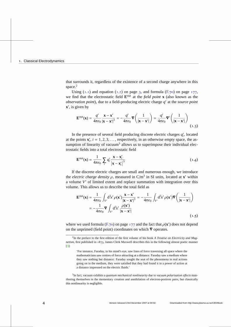
FIGURE1.2: Coulomb’s law for a distribution of individual chargesq′i localisedwithin a volumeV′ of limited extent.
We emphasise that under the assumption of linear superposition, equa-tion (1.5) on page4 is valid for an arbitrary distribution of electric charges,in-cluding discrete charges, in which caseρ is expressed in terms of Dirac deltadistributions:
ρ(x′) =∑i
q′i δ(x′ − x′i ) (1.6)
as illustrated in figure1.2. Inserting this expression into expression (1.5) on page4we recover expression (1.4) on page4.
Taking the divergence of the generalEstat expression for an arbitrary electriccharge distribution, equation (1.5) on page4, and using the representation of theDirac delta distribution, formula (F.73) on page177, we find that
∇ · Estat(x) = ∇ · 14πε0
∫
V′d3x′ ρ(x′)
x − x′
|x − x′|3
= − 14πε0
∫
V′d3x′ ρ(x′)∇ · ∇
(1
|x − x′|
)
= − 14πε0
∫
V′d3x′ ρ(x′)∇2
(1
|x − x′|
)
=1ε0
∫
V′d3x′ ρ(x′) δ(x − x′) =
ρ(x)ε0
(1.7)
which is the differential form ofGauss’s law of electrostatics.Since, according to formula (F.62) on page177, ∇ × [∇α(x)] ≡ 0 for any 3D
Downloaded from http://www.plasma.uu.se/CED/Book Version released 23rd December 2007 at 00:02. 5
1. Classical Electrodynamics
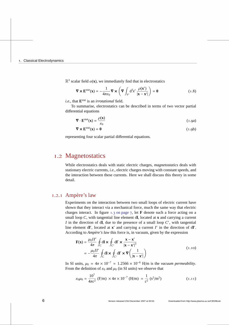
R3 scalar fieldα(x), we immediately find that in electrostatics
∇ × Estat(x) = − 14πε0
∇ ×
(
∇
∫
V′d3x′
ρ(x′)|x − x′|
)
= 0 (1.8)
i.e., thatEstat is anirrotational field.To summarise, electrostatics can be described in terms of two vector partial
differential equations
∇ · Estat(x) =ρ(x)ε0
(1.9a)
∇ × Estat(x) = 0 (1.9b)
representing four scalar partial differential equations.
1.2 MagnetostaticsWhile electrostatics deals with static electric charges,magnetostaticsdeals withstationary electric currents,i.e., electric charges moving with constant speeds, andthe interaction between these currents. Here we shall discuss this theory in somedetail.
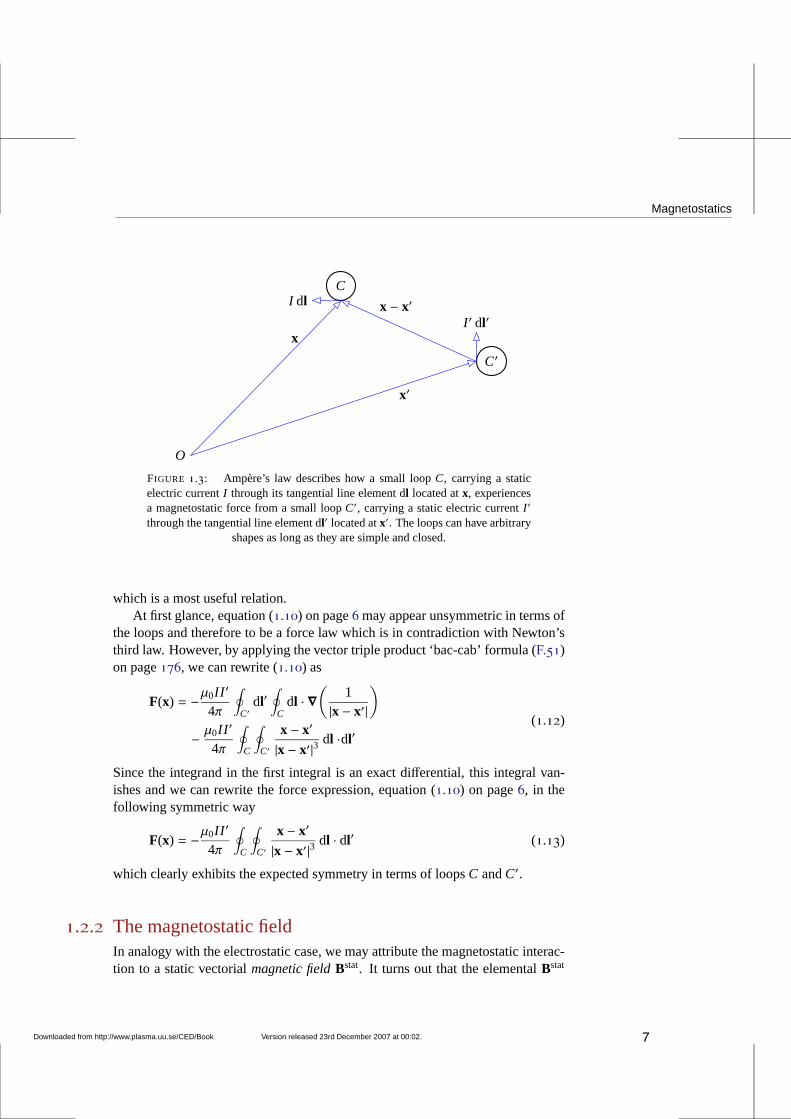
1.2.1 Ampère’s lawExperiments on the interaction between two small loops of electric current haveshown that they interact via a mechanical force, much the same way that electriccharges interact. In figure1.3 on page7, let F denote such a force acting on asmall loopC, with tangential line element dl, located atx and carrying a currentI in the direction of dl, due to the presence of a small loopC′, with tangentialline element dl′, located atx′ and carrying a currentI ′ in the direction of dl′.According toAmpère’s lawthis force is, in vacuum, given by the expression
F(x) =µ0II ′
4π
∮
Cdl ×
∮
C′dl′ ×
x − x′
|x − x′|3
= −µ0II ′
4π
∮
Cdl ×
∮
C′dl′ × ∇
(1
|x − x′|
) (1.10)
In SI units,µ0 = 4π × 10−7 ≈ 1.2566× 10⁻⁶ H/m is thevacuum permeability.From the definition ofε0 andµ0 (in SI units) we observe that
ε0µ0 =107
4πc2(F/m) × 4π × 10−7 (H/m) =
1c2
(s2/m2) (1.11)
6 Version released 23rd December 2007 at 00:02. Downloaded from http://www.plasma.uu.se/CED/Book
Magnetostatics
C′
C
I ′ dl′I dl
O
x′
x − x′
x
FIGURE 1.3: Ampère’s law describes how a small loopC, carrying a staticelectric currentI through its tangential line element dl located atx, experiencesa magnetostatic force from a small loopC′, carrying a static electric currentI ′
through the tangential line element dl′ located atx′. The loops can have arbitraryshapes as long as they are simple and closed.
which is a most useful relation.At first glance, equation (1.10) on page6may appear unsymmetric in terms of
the loops and therefore to be a force law which is in contradiction with Newton’sthird law. However, by applying the vector triple product ‘bac-cab’ formula (F.51)on page176, we can rewrite (1.10) as
F(x) = −µ0II ′
4π
∮
C′dl′∮
Cdl · ∇
(1
|x − x′|
)
− µ0II ′
4π
∮
C
∮
C′
x − x′
|x − x′|3dl ·dl′
(1.12)
Since the integrand in the first integral is an exact differential, this integral van-ishes and we can rewrite the force expression, equation (1.10) on page6, in thefollowing symmetric way
F(x) = −µ0II ′
4π
∮
C
∮
C′
x − x′
|x − x′|3dl · dl′ (1.13)
which clearly exhibits the expected symmetry in terms of loopsC andC′.
1.2.2 The magnetostatic fieldIn analogy with the electrostatic case, we may attribute themagnetostatic interac-tion to a static vectorialmagnetic fieldBstat. It turns out that the elementalBstat
Downloaded from http://www.plasma.uu.se/CED/Book Version released 23rd December 2007 at 00:02. 7

1. Classical Electrodynamics
can be defined as
dBstat(x)def≡ µ0I ′
4πdl′ ×
x − x′
|x − x′|3(1.14)
which expresses the small element dBstat(x) of the static magnetic field set up atthe field pointx by a small line element dl′ of stationary currentI ′ at the sourcepoint x′. The SI unit for the magnetic field, sometimes called themagnetic fluxdensityor magnetic induction, is Tesla (T).
If we generalise expression (1.14) to an integrated steady stateelectric currentdensityj (x), measured in A/m2 in SI units, we obtainBiot-Savart’s law:
Bstat(x) =µ0
4π
∫
V′d3x′ j (x′) ×
x − x′
|x − x′|3= − µ0
4π
∫
V′d3x′ j (x′) × ∇
(1
|x − x′|
)
=µ0
4π∇ ×
∫
V′d3x′
j (x′)|x − x′|
(1.15)
where we used formula (F.70) on page177, formula (F.57) on page177, and thefact thatj (x′) does not depend on the unprimed coordinates on which∇ operates.Comparing equation (1.5) on page4 with equation (1.15), we see that there existsa close analogy between the expressions forEstat and Bstat but that they differin their vectorial characteristics. With this definition ofBstat, equation (1.10) onpage6 may we written
F(x) = I∮
Cdl × Bstat(x) (1.16)
In order to assess the properties ofBstat, we determine its divergence and curl.Taking the divergence of both sides of equation (1.15) and utilising formula (F.63)on page177, we obtain
∇ · Bstat(x) =µ0
4π∇ ·(
∇ ×
∫
V′d3x′
j (x′)|x − x′|
)
= 0 (1.17)
since, according to formula (F.63) on page177,∇ · (∇×a) vanishes for any vectorfield a(x).
Applying the operator ‘bac-cab’ rule, formula (F.64) on page177, the curl ofequation (1.15) can be written
∇ × Bstat(x) =µ0
4π∇ ×
(
∇ ×
∫
V′d3x′
j (x′)|x − x′|
)
=
= − µ0
4π
∫
V′d3x′ j (x′)∇2
(1
|x − x′|
)
+µ0
4π
∫
V′d3x′ [j (x′) · ∇′] ∇′
(1
|x − x′|
)
(1.18)
8 Version released 23rd December 2007 at 00:02. Downloaded from http://www.plasma.uu.se/CED/Book
Electrodynamics
In the first of the two integrals on the right-hand side, we usethe representationof the Dirac delta function given in formula (F.73) on page177, and integrate thesecond one by parts, by utilising formula (F.56) on page177 as follows:
∫
V′d3x′ [j (x′) · ∇′]∇′
(1
|x − x′|
)
= xk
∫
V′d3x′ ∇′ ·
j (x′)[∂
∂x′k
(1
|x − x′|
)]
−∫
V′d3x′
[∇′ · j (x′)
]∇′(
1|x − x′|
)
= xk
∫
S′d2x′ n′ · j (x′) ∂
∂x′k
(1
|x − x′|
)
−∫
V′d3x′
[∇′ · j (x′)
]∇′(
1|x − x′|
)
(1.19)
Then we note that the first integral in the result, obtained byapplying Gauss’stheorem, vanishes when integrated over a large sphere far away from the localisedsourcej (x′), and that the second integral vanishes because∇ · j = 0 for stationarycurrents (no charge accumulation in space). The net result is simply
∇ × Bstat(x) = µ0
∫
V′d3x′ j (x′)δ(x − x′) = µ0j (x) (1.20)
1.3 ElectrodynamicsAs we saw in the previous sections, the laws of electrostatics and magnetostaticscan be summarised in two pairs of time-independent, uncoupled vector partialdifferential equations, namely theequations of classical electrostatics
∇ · Estat(x) =ρ(x)ε0
(1.21a)
∇ × Estat(x) = 0 (1.21b)
and theequations of classical magnetostatics
∇ · Bstat(x) = 0 (1.22a)
∇ × Bstat(x) = µ0j (x) (1.22b)
Since there is nothinga priori which connectsEstat directly with Bstat, we mustconsider classical electrostatics and classical magnetostatics as two independenttheories.
Downloaded from http://www.plasma.uu.se/CED/Book Version released 23rd December 2007 at 00:02. 9
1. Classical Electrodynamics
However, when we include time-dependence, these theories are unified intoone theory,classical electrodynamics. This unification of the theories of electric-ity and magnetism is motivated by two empirically established facts:
1. Electric charge is a conserved quantity and electric current is a transport ofelectric charge. This fact manifests itself in the equationof continuity and,as a consequence, in Maxwell’s displacement current.
2. A change in the magnetic flux through a loop will induce an EMFelectricfield in the loop. This is the celebrated Faraday’s law of induction.
1.3.1 Equation of continuity for electric chargeLet j (t, x) denote the time-dependent electric current density. In the simplest caseit can be defined asj = vρ wherev is the velocity of the electric charge den-sity ρ. In general,j has to be defined in statistical mechanical terms asj (t, x) =∑α qα
∫
d3v v fα(t, x, v) where fα(t, x, v) is the (normalised) distribution function forparticle speciesα with electric chargeqα.
The electric charge conservation lawcan be formulated in theequation ofcontinuity
∂ρ(t, x)∂t
+ ∇ · j (t, x) = 0 (1.23)
which states that the time rate of change of electric chargeρ(t, x) is balanced by adivergence in the electric current densityj (t, x).
1.3.2 Maxwell’s displacement currentWe recall from the derivation of equation (1.20) on page9 that there we used thefact that in magnetostatics∇ · j (x) = 0. In the case of non-stationary sourcesand fields, we must, in accordance with the continuity equation (1.23), set∇ ·j (t, x) = −∂ρ(t, x)/∂t. Doing so, and formally repeating the steps in the derivationof equation (1.20) on page9, we would obtain the formal result
∇ × B(t, x) = µ0
∫
V′d3x′ j (t, x′)δ(x − x′) +
µ0
4π∂
∂t
∫
V′d3x′ ρ(t, x′)∇′
(1
|x − x′|
)
= µ0j (t, x) + µ0∂
∂tε0E(t, x)
(1.24)
10 Version released 23rd December 2007 at 00:02. Downloaded from http://www.plasma.uu.se/CED/Book
Electrodynamics
where, in the last step, we have assumed that a generalisation of equation (1.5) onpage4 to time-varying fields allows us to make the identification4
14πε0
∂
∂t
∫
V′d3x′ ρ(t, x′)∇′
(1
|x − x′|
)
=∂
∂t
[
− 14πε0
∫
V′d3x′ ρ(t, x′)∇
(1
|x − x′|
)]
=∂
∂t
[
− 14πε0
∇
∫
V′d3x′
ρ(t, x′)|x − x′|
]
=∂
∂tE(t, x)
(1.25)
The result is Maxwell’s source equation for theB field
∇ × B(t, x) = µ0
(
j (t, x) +∂
∂tε0E(t, x)
)
= µ0j (t, x) +1c2
∂
∂tE(t, x) (1.26)
where the last term∂ε0E(t, x)/∂t is the famousdisplacement current. This termwas introduced, in a stroke of genius, by Maxwell [8] in order to make the righthand side of this equation divergence free whenj (t, x) is assumed to represent thedensity of the total electric current, which can be split up in ‘ordinary’ conduc-tion currents, polarisation currents and magnetisation currents. The displacementcurrent is an extra term which behaves like a current densityflowing in vacuum.As we shall see later, its existence has far-reaching physical consequences as itpredicts the existence of electromagnetic radiation that can carry energy and mo-mentum over very long distances, even in vacuum.
1.3.3 Electromotive forceIf an electric fieldE(t, x) is applied to a conducting medium, a current densityj (t, x) will be produced in this medium. There exist also hydrodynamical andchemical processes which can create currents. Under certain physical conditions,and for certain materials, one can sometimes assume, that, as a first approxima-tion, a linear relationship exists between the electric current densityj andE. Thisapproximation is calledOhm’s law:
j (t, x) = σE(t, x) (1.27)
whereσ is theelectric conductivity(S/m). In the most general cases, for instancein an anisotropic conductor,σ is a tensor.
We can view Ohm’s law, equation (1.27) above, as the first term in a Taylorexpansion of the lawj [E(t, x)]. This general law incorporatesnon-linear effects
4Later, we will need to consider this generalisation and formal identification further.
Downloaded from http://www.plasma.uu.se/CED/Book Version released 23rd December 2007 at 00:02. 11
1. Classical Electrodynamics
such as frequency mixing. Examples of media which are highlynon-linear aresemiconductors and plasma. We draw the attention to the factthat even in caseswhen the linear relation betweenE and j is a good approximation, we still haveto use Ohm’s law with care. The conductivityσ is, in general, time-dependent(temporal dispersive media) but then it is often the case that equation (1.27) onpage11 is valid for each individual Fourier component of the field.
If the current is caused by an applied electric fieldE(t, x), this electric fieldwill exert work on the charges in the medium and, unless the medium is super-conducting, there will be some energy loss. The rate at whichthis energy is ex-pended isj · E per unit volume. IfE is irrotational (conservative),j will decayaway with time. Stationary currents therefore require thatan electric field whichcorresponds to anelectromotive force (EMF)is present. In the presence of such afield EEMF, Ohm’s law, equation (1.27) on page11, takes the form
j = σ(Estat+ EEMF) (1.28)
The electromotive force is defined as
E =∮
Cdl · (Estat+ EEMF) (1.29)
where dl is a tangential line element of the closed loopC.
1.3.4 Faraday’s law of inductionIn subsection1.1.2 we derived the differential equations for the electrostatic field.In particular, on page6we derived equation (1.8) which states that∇ × Estat(x) = 0and thus thatEstat is a conservative field(it can be expressed as a gradient of ascalar field). This implies that the closed line integral ofEstat in equation (1.29)above vanishes and that this equation becomes
E =∮
Cdl · EEMF (1.30)
It has been established experimentally that a nonconservative EMF field isproduced in a closed circuitC at rest if the magnetic flux through this circuit varieswith time. This is formulated inFaraday’s lawwhich, in Maxwell’s generalisedform, reads
E(t) =∮
Cdl · E(t, x) = − d
dtΦm(t)
= − ddt
∫
Sd2x n · B(t, x) = −
∫
Sd2x n · ∂
∂tB(t, x)
(1.31)
12 Version released 23rd December 2007 at 00:02. Downloaded from http://www.plasma.uu.se/CED/Book
Electrodynamics
d2x n
B(x) B(x)
v
dlC
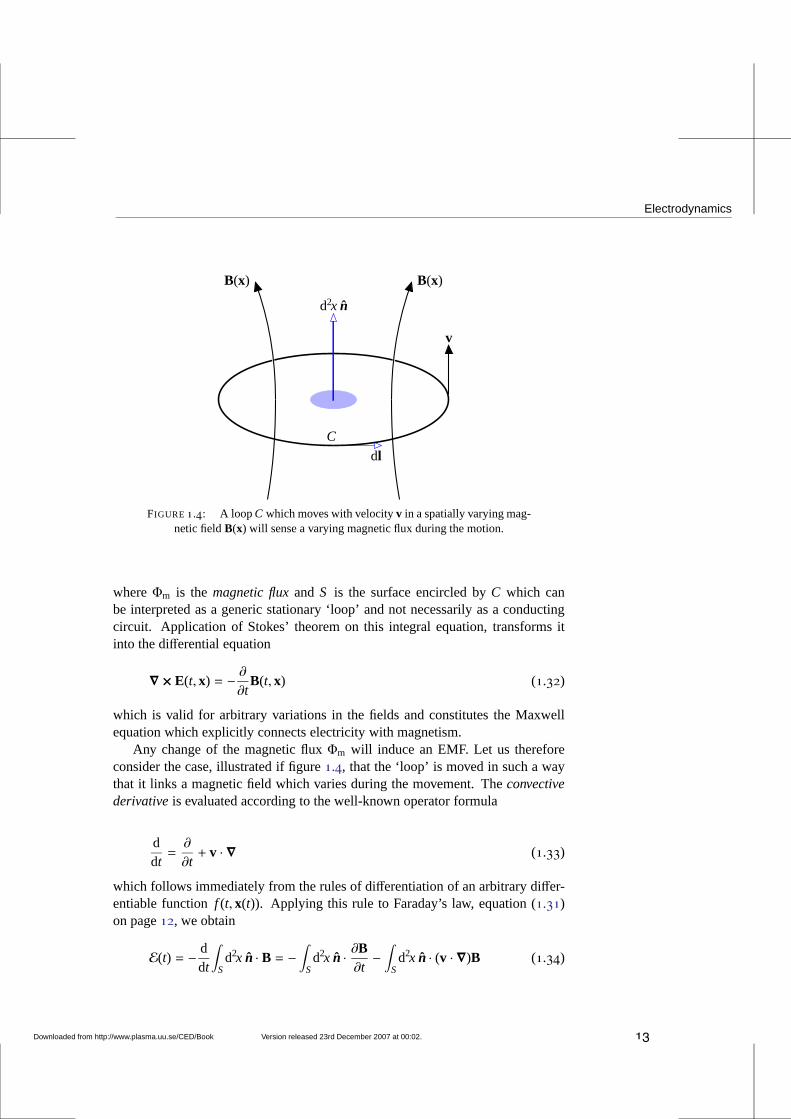
FIGURE1.4: A loopC which moves with velocityv in a spatially varying mag-netic fieldB(x) will sense a varying magnetic flux during the motion.
whereΦm is the magnetic fluxand S is the surface encircled byC which canbe interpreted as a generic stationary ‘loop’ and not necessarily as a conductingcircuit. Application of Stokes’ theorem on this integral equation, transforms itinto the differential equation
∇ × E(t, x) = − ∂∂t
B(t, x) (1.32)
which is valid for arbitrary variations in the fields and constitutes the Maxwellequation which explicitly connects electricity with magnetism.
Any change of the magnetic fluxΦm will induce an EMF. Let us thereforeconsider the case, illustrated if figure1.4, that the ‘loop’ is moved in such a waythat it links a magnetic field which varies during the movement. Theconvectivederivativeis evaluated according to the well-known operator formula
ddt=∂
∂t+ v · ∇ (1.33)
which follows immediately from the rules of differentiation of an arbitrary differ-entiable functionf (t, x(t)). Applying this rule to Faraday’s law, equation (1.31)on page12, we obtain
E(t) = − ddt
∫
Sd2x n · B = −
∫
Sd2x n · ∂B
∂t−∫
Sd2x n · (v · ∇)B (1.34)
Downloaded from http://www.plasma.uu.se/CED/Book Version released 23rd December 2007 at 00:02. 13
1. Classical Electrodynamics
During spatial differentiationv is to be considered as constant, and equa-tion (1.17) on page8 holds also for time-varying fields:
∇ · B(t, x) = 0 (1.35)
(it is one of Maxwell’s equations) so that, according to formula (F.59) on page177,
∇ × (B × v) = (v · ∇)B (1.36)
allowing us to rewrite equation (1.34) on page13 in the following way:
E(t) =∮
Cdl · EEMF = − d
dt
∫
Sd2x n · B
= −∫
Sd2x n · ∂B
∂t−∫
Sd2x n · ∇ × (B × v)
(1.37)
With Stokes’ theorem applied to the last integral, we finallyget
E(t) =∮
Cdl · EEMF = −
∫
Sd2x n · ∂B
∂t−∮
Cdl · (B × v) (1.38)
or, rearranging the terms,∮
Cdl · (EEMF − v × B) = −
∫
Sd2x n · ∂B
∂t(1.39)
whereEEMF is the field which is induced in the ‘loop’,i.e., in themovingsystem.The use of Stokes’ theorem ‘backwards’ on equation (1.39) above yields
∇ × (EEMF − v × B) = −∂B∂t
(1.40)
In thefixedsystem, an observer measures the electric field
E = EEMF − v × B (1.41)
Hence, a moving observer measures the followingLorentz forceon a chargeq
qEEMF = qE + q(v × B) (1.42)
corresponding to an ‘effective’ electric field in the ‘loop’ (moving observer)
EEMF = E + v × B (1.43)
Hence, we can conclude that for astationaryobserver, the Maxwell equation
∇ × E = −∂B∂t
(1.44)
is indeed valid even if the ‘loop’ is moving.
14 Version released 23rd December 2007 at 00:02. Downloaded from http://www.plasma.uu.se/CED/Book
Electrodynamics
1.3.5 Maxwell’s microscopic equationsWe are now able to collect the results from the above considerations and formulatethe equations of classical electrodynamics valid for arbitrary variations in time andspace of the coupled electric and magnetic fieldsE(t, x) andB(t, x). The equationsare
∇ · E = ρ
ε0(1.45a)
∇ × E = −∂B∂t
(1.45b)
∇ · B = 0 (1.45c)
∇ × B = ε0µ0∂E∂t+ µ0j (t, x) (1.45d)
In these equationsρ(t, x) represents the total, possibly both time and space depen-dent, electric charge,i.e., free as well as induced (polarisation) charges, andj (t, x)represents the total, possibly both time and space dependent, electric current,i.e.,conduction currents (motion of free charges) as well as all atomistic (polarisation,magnetisation) currents. As they stand, the equations therefore incorporate theclassical interaction between all electric charges and currents in the system andare calledMaxwell’s microscopic equations. Another name often used for themis theMaxwell-Lorentz equations. Together with the appropriateconstitutive re-lations, which relateρ andj to the fields, and the initial and boundary conditionspertinent to the physical situation at hand, they form a system of well-posed partialdifferential equations which completely determineE andB.
1.3.6 Maxwell’s macroscopic equationsThe microscopic field equations (1.45) provide a correct classical picture for arbi-trary field and source distributions, including both microscopic and macroscopicscales. However, for macroscopic substances it is sometimes convenient to intro-duce new derived fields which represent the electric and magnetic fields in which,in an average sense, the material properties of the substances are already included.These fields are theelectric displacementD and themagnetising fieldH. In themost general case, these derived fields are complicated nonlocal, nonlinear func-tionals of the primary fieldsE andB:
D = D[t, x; E,B] (1.46a)
H = H[t, x; E,B] (1.46b)
Under certain conditions, for instance for very low field strengths, we may assumethat the response of a substance to the fields may be approximated as a linear one
Downloaded from http://www.plasma.uu.se/CED/Book Version released 23rd December 2007 at 00:02. 15
1. Classical Electrodynamics
so that
D = εE (1.47)
H = µ−1B (1.48)
i.e., that the derived fields are linearly proportional to the primary fields and thatthe electric displacement (magnetising field) is only dependent on the electric(magnetic) field.
The field equations expressed in terms of the derived field quantitiesD andHare
∇ · D = ρ(t, x) (1.49a)
∇ × E = −∂B∂t
(1.49b)
∇ · B = 0 (1.49c)
∇ × H =∂D∂t+ j (t, x) (1.49d)
and are calledMaxwell’s macroscopic equations. We will study them in moredetail in chapter4.
1.4 Electromagnetic dualityIf we look more closely at the microscopic Maxwell equations (1.45), we see thatthey exhibit a certain, albeit not complete, symmetry. Let us follow Dirac andmake thead hocassumption that there existmagnetic monopolesrepresented bya magnetic charge density, which we denote byρm = ρm(t, x), and amagneticcurrent density, which we denote byjm = jm(t, x). With these new quantities in-cluded in the theory, and with the electric charge density denotedρe and the elec-tric current density denotedje, the Maxwell equations will be symmetrised intothe following two scalar and two vector, coupled, partial differential equations:
∇ · E = ρe
ε0(1.50a)
∇ × E = −∂B∂t− µ0jm (1.50b)
∇ · B = µ0ρm (1.50c)
∇ × B = ε0µ0∂E∂t+ µ0je (1.50d)
16 Version released 23rd December 2007 at 00:02. Downloaded from http://www.plasma.uu.se/CED/Book
Electromagnetic duality
We shall call these equationsDirac’s symmetrised Maxwell equationsor theelec-tromagnetodynamic equations.
Taking the divergence of (1.50b), we find that
∇ · (∇ × E) = − ∂∂t
(∇ · B) − µ0∇ · jm ≡ 0 (1.51)
where we used the fact that, according to formula (F.63) on page177, the diver-gence of a curl always vanishes. Using (1.50c) to rewrite this relation, we obtainthemagnetic monopole equation of continuity
∂ρm
∂t+ ∇ · jm = 0 (1.52)
which has the same form as that for the electric monopoles (electric charges) andcurrents, equation (1.23) on page10.
We notice that the new equations (1.50) on page16 exhibit the following sym-metry (recall thatε0µ0 = 1/c2):
E→ cB (1.53a)
cB→ −E (1.53b)
cρe→ ρm (1.53c)
ρm→ −cρe (1.53d)
cje→ jm (1.53e)
jm→ −cje (1.53f)
which is a particular case (θ = π/2) of the generalduality transformation, alsoknown as theHeaviside-Larmor-Rainich transformation(indicted by theHodgestar operator⋆)
⋆E = E cosθ + cB sinθ (1.54a)
c⋆B = −E sinθ + cB cosθ (1.54b)
c⋆ρe = cρe cosθ + ρm sinθ (1.54c)⋆ρm = −cρe sinθ + ρm cosθ (1.54d)
c⋆je = cje cosθ + jm sinθ (1.54e)⋆jm = −cje sinθ + jm cosθ (1.54f)
which leaves the symmetrised Maxwell equations, and hence the physics theydescribe (often referred to aselectromagnetodynamics), invariant. SinceE andje
are (true or polar) vectors,B a pseudovector (axial vector),ρe a (true) scalar, thenρm andθ, which behaves as amixing anglein a two-dimensional ‘charge space’,must be pseudoscalars andjm a pseudovector.
Downloaded from http://www.plasma.uu.se/CED/Book Version released 23rd December 2007 at 00:02. 17
1. Classical Electrodynamics
The invariance of Dirac’s symmetrised Maxwell equations under the similaritytransformation means that the amount of magnetic monopole densityρm is irrele-vant for the physics as long as the ratioρm/ρe = tanθ is kept constant. So whetherwe assume that the particles are only electrically charged or have also a magneticcharge with a given, fixed ratio between the two types of charges is a matter ofconvention, as long as we assume that this fraction isthe same for all particles.Such particles are referred to asdyons[14]. By varying the mixing angleθ we canchange the fraction of magnetic monopoles at will without changing the laws ofelectrodynamics. Forθ = 0 we recover the usual Maxwell electrodynamics as weknow it.5
1.5 Bibliography[1] T. W. BARRETT AND D. M. GRIMES, Advanced Electromagnetism. Foundations, Theory
and Applications, World Scientific Publishing Co., Singapore, 1995, ISBN 981-02-2095-2.
[2] R. BECKER, Electromagnetic Fields and Interactions, Dover Publications, Inc.,New York, NY, 1982, ISBN 0-486-64290-9.
[3] W. GREINER, Classical Electrodynamics, Springer-Verlag, New York, Berlin, Heidel-berg, 1996, ISBN 0-387-94799-X.
[4] E. HALLÉN , Electromagnetic Theory, Chapman & Hall, Ltd., London, 1962.
[5] J. D. JACKSON, Classical Electrodynamics, third ed., John Wiley & Sons, Inc.,New York, NY . . . , 1999, ISBN 0-471-30932-X.
[6] L. D. LANDAU AND E. M. LIFSHITZ, The Classical Theory of Fields, fourth revisedEnglish ed., vol. 2 ofCourse of Theoretical Physics, Pergamon Press, Ltd., Oxford . . . ,1975, ISBN 0-08-025072-6.
[7] F. E. LOW, Classical Field Theory, John Wiley & Sons, Inc., New York, NY . . . , 1997,ISBN 0-471-59551-9.
[8] J. C. MAXWELL , A dynamical theory of the electromagnetic field,Royal Society Trans-actions, 155(1864).11
5As Julian Schwinger (1918–1994) put it [15]:
‘. . . there are strong theoretical reasons to believe that magnetic charge exists in nature,and may have played an important role in the development of the universe. Searches formagnetic charge continue at the present time, emphasising that electromagnetism is veryfar from being a closed object’.
18 Version released 23rd December 2007 at 00:02. Downloaded from http://www.plasma.uu.se/CED/Book
Bibliography
[9] J. C. MAXWELL , A Treatise on Electricity and Magnetism, third ed., vol. 1, Dover Publi-cations, Inc., New York, NY, 1954, ISBN 0-486-60636-8.4
[10] J. C. MAXWELL , A Treatise on Electricity and Magnetism, third ed., vol. 2, Dover Publi-cations, Inc., New York, NY, 1954, ISBN 0-486-60637-8.
[11] D. B. MELROSE ANDR. C. MCPHEDRAN, Electromagnetic Processes in Dispersive Me-dia, Cambridge University Press, Cambridge . . . , 1991, ISBN 0-521-41025-8.
[12] W. K. H. PANOFSKY AND M. PHILLIPS, Classical Electricity and Magnetism, second ed.,Addison-Wesley Publishing Company, Inc., Reading, MA . . . ,1962, ISBN 0-201-05702-6.
[13] F. ROHRLICH, Classical Charged Particles, Perseus Books Publishing, L.L.C., Reading,MA . . . , 1990, ISBN 0-201-48300-9.
[14] J. SCHWINGER, A magnetic model of matter,Science, 165(1969), pp. 757–761.18
[15] J. SCHWINGER, L. L. DERAAD , JR., K. A. M ILTON , AND W. TSAI, Classical Electrody-namics, Perseus Books, Reading, MA, 1998, ISBN 0-7382-0056-5.18, 121
[16] J. A. STRATTON, Electromagnetic Theory, McGraw-Hill Book Company, Inc., NewYork, NY and London, 1953, ISBN 07-062150-0.
[17] J. VANDERLINDE, Classical Electromagnetic Theory, John Wiley & Sons, Inc., NewYork, Chichester, Brisbane, Toronto, and Singapore, 1993,ISBN 0-471-57269-1.
Downloaded from http://www.plasma.uu.se/CED/Book Version released 23rd December 2007 at 00:02. 19
1. Classical Electrodynamics
1.6 Examples
⊲FARADAY ’ S LAW AS A CONSEQUENCE OF CONSERVATION OF MAGNETIC CHARGEEXAMPLE 1.1
Postulate1.1 (Indestructibility of magnetic charge). Magnetic charge exists and is indestruc-tible in the same way that electric charge exists and is indestructible. In other words wepostu-latethat there exists an equation of continuity for magnetic charges:
∂ρm(t, x)∂t
+ ∇ · jm(t, x) = 0
Use this postulate and Dirac’s symmetrised form of Maxwell’s equations to derive Fara-day’s law.
The assumption of the existence of magnetic charges suggests a Coulomb-like law for mag-netic fields:
Bstat(x) =µ0
4π
∫
V′d3x′ ρm(x′)
x − x′
|x − x′|3= − µ0
4π
∫
V′d3x′ ρm(x′)∇
(1
|x − x′|
)
= − µ0
4π∇
∫
V′d3x′
ρm(x′)|x − x′|
(1.55)
[cf. equation (1.5) on page4 for Estat] and, if magnetic currents exist, a Biot-Savart-like law forelectric fields [cf. equation (1.15) on page8 for Bstat]:
Estat(x) = − µ0
4π
∫
V′d3x′ jm(x′) ×
x − x′
|x − x′|3=µ0
4π
∫
V′d3x′ jm(x′) × ∇
(1
|x − x′|
)
= − µ0
4π∇ ×
∫
V′d3x′
jm(x′)|x − x′|
(1.56)
Taking the curl of the latter and using the operator ‘bac-cab’ rule, formula (F.59) on page177,we find that
∇ × Estat(x) = − µ0
4π∇ ×
(
∇ ×
∫
V′d3x′
jm(x′)|x − x′|
)
=
=µ0
4π
∫
V′d3x′ jm(x′)∇2
(1
|x − x′|
)
− µ0
4π
∫
V′d3x′ [jm(x′) · ∇′]∇′
(1
|x − x′|
) (1.57)
Comparing with equation (1.18) on page8 for Estat and the evaluation of the integrals there, weobtain
∇ × Estat(x) = −µ0
∫
V′d3x′ jm(x′) δ(x − x′) = −µ0jm(x) (1.58)
We assume that formula (1.56) above is valid also for time-varying magnetic currents.Then, with the use of the representation of the Dirac delta function, equation (F.73) on page177,the equation of continuity for magnetic charge, equation (1.52) on page17, and the assumptionof the generalisation of equation (1.55) to time-dependent magnetic charge distributions, weobtain, formally,
20 Version released 23rd December 2007 at 00:02. Downloaded from http://www.plasma.uu.se/CED/Book
Examples
∇ × E(t, x) = −µ0
∫
V′d3x′ jm(t, x′)δ(x − x′) − µ0
4π∂
∂t
∫
V′d3x′ ρm(t, x′)∇′
(1
|x − x′|
)
= −µ0jm(t, x) − ∂
∂tB(t, x)
(1.59)
[cf. equation (1.24) on page10] which we recognise as equation (1.50b) on page16. A trans-formation of this electromagnetodynamic result by rotating into the ‘electric realm’ of chargespace, thereby lettingjm tend to zero, yields the electrodynamic equation (1.50b) on page16,i.e., the Faraday law in the ordinary Maxwell equations. This process also provides an alter-native interpretation of the term∂B/∂t as amagnetic displacement current, dual to theelectricdisplacement current[cf. equation (1.26) on page11].
By postulating the indestructibility of a hypothetical magnetic charge, we have thereby beenable to replace Faraday’s experimental results on electromotive forces and induction in loops asa foundation for the Maxwell equations by a more appealing one.
⊳ END OF EXAMPLE 1.1
⊲DUALITY OF THE ELECTROMAGNETODYNAMIC EQUATIONS EXAMPLE 1.2
Show that the symmetric, electromagnetodynamic form of Maxwell’s equations (Dirac’ssymmetrised Maxwell equations), equations (1.50) on page16, are invariant under the dualitytransformation (1.54).
Explicit application of the transformation yields
∇ · ⋆E = ∇ · (E cosθ + cB sinθ) =ρe
ε0cosθ + cµ0ρ
m sinθ
=1ε0
(
ρe cosθ +1cρm sinθ
)
=⋆ρe
ε0
(1.60)
∇ ×⋆E +
∂⋆B∂t= ∇ × (E cosθ + cB sinθ) +
∂
∂t
(
−1c
E sinθ + B cosθ
)
= −µ0jm cosθ − ∂B∂t
cosθ + cµ0j e sinθ +1c∂E∂t
sinθ
− 1c∂E∂t
sinθ +∂B∂t
cosθ = −µ0jm cosθ + cµ0j e sinθ
= −µ0(−cj e sinθ + jm cosθ) = −µ0⋆jm
(1.61)
∇ · ⋆B = ∇ · (−1c
E sinθ + B cosθ) = − ρe
cε0sinθ + µ0ρ
m cosθ
= µ0 (−cρe sinθ + ρm cosθ) = µ0⋆ρm
(1.62)
Downloaded from http://www.plasma.uu.se/CED/Book Version released 23rd December 2007 at 00:02. 21
1. Classical Electrodynamics
∇ ×⋆B − 1
c2
∂⋆E∂t= ∇ × (−1
cE sinθ + B cosθ) − 1
c2
∂
∂t(E cosθ + cB sinθ)
=1cµ0jm sinθ +
1c∂B∂t
cosθ + µ0j e cosθ +1c2
∂E∂t
cosθ
− 1c2
∂E∂t
cosθ − 1c∂B∂t
sinθ
= µ0
(1c
jm sinθ + j e cosθ
)
= µ0⋆j e
(1.63)
QED
⊳ END OF EXAMPLE 1.2
⊲DIRAC’ S SYMMETRISEDMAXWELL EQUATIONS FOR A FIXED MIXING ANGLEEXAMPLE 1.3
Show that for a fixed mixing angleθ such that
ρm = cρe tanθ (1.64a)
jm = cj e tanθ (1.64b)
the symmetrised Maxwell equations reduce to the usual Maxwell equations.
Explicit application of the fixed mixing angle conditions onthe duality transformation(1.54) on page17 yields
⋆ρe = ρe cosθ +1cρm sinθ = ρe cosθ +
1c
cρe tanθ sinθ
=1
cosθ(ρe cos2 θ + ρe sin2 θ) =
1cosθ
ρe(1.65a)
⋆ρm = −cρe sinθ + cρe tanθ cosθ = −cρe sinθ + cρe sinθ = 0 (1.65b)
⋆j e = j e cosθ + j e tanθ sinθ =1
cosθ(j e cos2 θ + j e sin2 θ) =
1cosθ
j e (1.65c)
⋆jm = −cj e sinθ + cj e tanθ cosθ = −cj e sinθ + cj e sinθ = 0 (1.65d)
Hence, a fixed mixing angle, or, equivalently, a fixed ratio between the electric and magneticcharges/currents, ‘hides’ the magnetic monopole influence (ρm and jm) on the dynamic equa-tions.
We notice that the inverse of the transformation given by equation (1.54) on page17 yields
E = ⋆E cosθ − c⋆B sinθ (1.66)
This means that
∇ · E = ∇ · ⋆E cosθ − c∇ · ⋆B sinθ (1.67)
Furthermore, from the expressions for the transformed charges and currents above, we find that
∇ · ⋆E =⋆ρe
ε0=
1cosθ
ρe
ε0(1.68)
22 Version released 23rd December 2007 at 00:02. Downloaded from http://www.plasma.uu.se/CED/Book
Examples
and
∇ · ⋆B = µ0⋆ρm = 0 (1.69)
so that
∇ · E = 1cosθ
ρe
ε0cosθ − 0 =
ρe
ε0(1.70)
and so on for the other equations. QED
⊳ END OF EXAMPLE 1.3
⊲COMPLEX FIELD SIX-VECTOR FORMALISM EXAMPLE 1.4
It is sometimes convenient to introduce thecomplex field six-vector, also known as theRiemann-Silberstein vector
G(t, x) = E(t, x) + icB(t, x) (1.71)
whereE,B ∈ R3 and henceG ∈ C3. One fundamental property ofC3 is that inner (scalar)products in this space are invariant just as they are inR3. However, as discussed in exam-ple M.3 on page195, the inner (scalar) product inC3 can be defined in two different ways.Considering the special case of the scalar product ofG with itself, we have the following twopossibilities of defining (the square of) the ‘length’ ofG:
1. The inner (scalar) product defined asG scalar multiplied with itself
G ·G = (E + icB) · (E + icB) = E2 − c2B2 + 2icE · B (1.72)
Since this is an invariant scalar quantity, we find that
E2 − c2B2 = Const (1.73a)
E · B = Const (1.73b)
2. The inner (scalar) product defined asG scalar multiplied with the complex conjugate ofitself
G ·G∗ = (E + icB) · (E − icB) = E2 + c2B2 (1.74)
which is also an invariant scalar quantity. As we shall see later, this quantity is propor-tional to the electromagnetic field energy, which indeed is aconserved quantity.
3. As with any vector, the cross product ofG with itself vanishes:
G ×G = (E + icB) × (E + icB)
= E × E − c2B × B + ic(E × B) + ic(B × E)
= 0+ 0+ ic(E × B) − ic(E × B) = 0
(1.75)
4. The cross product ofG with the complex conjugate of itself
Downloaded from http://www.plasma.uu.se/CED/Book Version released 23rd December 2007 at 00:02. 23
1. Classical Electrodynamics
G ×G∗ = (E + icB) × (E − icB)
= E × E + c2B × B − ic(E × B) + ic(B × E)
= 0+ 0− ic(E × B) − ic(E × B) = −2ic(E × B)
(1.76)
is proportional to the electromagnetic power flux, to be introduced later.
⊳ END OF EXAMPLE 1.4
⊲DUALITY EXPRESSED IN THE COMPLEX FIELD SIX-VECTOREXAMPLE 1.5
Expressed in the Riemann-Silberstein complex field vector,introduced in exam-ple1.4 on page23, the duality transformation equations (1.54) on page17 become
⋆G = ⋆E + ic⋆B = E cosθ + cB sinθ − iE sinθ + icB cosθ
= E(cosθ − i sinθ) + icB(cosθ − i sinθ) = e−iθ(E + icB) = e−iθG(1.77)
from which it is easy to see that
⋆G · ⋆G∗ =∣∣⋆G∣∣2= e−iθG · eiθG∗ = |G|2 (1.78)
while
⋆G · ⋆G = e−2iθG ·G (1.79)
Furthermore, assuming thatθ = θ(t, x), we see that the spatial and temporal differentiationof ⋆G leads to
∂t⋆G ≡ ∂⋆G
∂t= −i(∂tθ)e−iθG + e−iθ∂tG (1.80a)
∂ · ⋆G ≡ ∇ · ⋆G = −ie−iθ∇θ ·G + e−iθ
∇ ·G (1.80b)
∂ × ⋆G ≡ ∇ × ⋆G = −ie−iθ∇θ ×G + e−iθ
∇ ×G (1.80c)
which means that∂t⋆G transforms as⋆G itself only if θ is time-independent, and that∇ · ⋆G
and∇ × ⋆G transform as⋆G itself only if θ is space-independent.
⊳ END OF EXAMPLE 1.5
24 Version released 23rd December 2007 at 00:02. Downloaded from http://www.plasma.uu.se/CED/Book
Downloaded from http://www.plasma.uu.se/CED/Book Version released 23rd December 2007 at 00:02.
2ELECTROMAGNETIC WAVES
In this chapter we investigate the dynamical properties of the electromagnetic fieldby deriving a set of equations which are alternatives to the Maxwell equations. Itturns out that these alternative equations are wave equations, indicating that elec-tromagnetic waves are natural and common manifestations ofelectrodynamics.
Maxwell’s microscopic equations [cf. equations (1.45) on page15] are
∇ · E = ρ(t, x)ε0
(Gauss’s law) (2.1a)
∇ × E = −∂B∂t
(Faraday’s law) (2.1b)
∇ · B = 0 (No free magnetic charges) (2.1c)
∇ × B = µ0j (t, x) + ε0µ0∂E∂t
(Maxwell’s law) (2.1d)
and can be viewed as an axiomatic basis for classical electrodynamics. They de-scribe, in scalar and vector differential equation form, the electric and magneticfieldsE andB produced by given, prescribed charge distributionsρ(t, x) and cur-rent distributionsj (t, x) with arbitrary time and space dependences.
However, as is well known from the theory of differential equations, these fourfirst order, coupled partial differential vector equations can be rewritten as two un-coupled, second order partial equations, one forE and one forB. We shall derivethese second order equations which, as we shall see arewave equations, and thendiscuss the implications of them. We show that for certain media, theB wave fieldcan be easily obtained from the solution of theE wave equation.
25
2. Electromagnetic Waves
2.1 The wave equationsWe restrict ourselves to derive the wave equations for the electric field vectorEand the magnetic field vectorB in an electrically neutral region,i.e., a volumewhere there is no net charge,ρ = 0, and no electromotive forceEEMF = 0.
2.1.1 The wave equation forEIn order to derive the wave equation forE we take the curl of (2.1b) and use (2.1d),to obtain
∇ × (∇ × E) = − ∂∂t
(∇ × B) = −µ0∂
∂t
(
j + ε0∂
∂tE)
(2.2)
According to the operator triple product ‘bac-cab’ rule equation (F.64) on page177
∇ × (∇ × E) = ∇(∇ · E) − ∇2E (2.3)
Furthermore, sinceρ = 0, equation (2.1a) on page25 yields
∇ · E = 0 (2.4)
and sinceEEMF = 0, Ohm’s law, equation (1.28) on page12, allows us to use theapproximation
j = σE (2.5)
we find that equation (2.2) above can be rewritten
∇2E − µ0∂
∂t
(
σE + ε0∂
∂tE)
= 0 (2.6)
or, also using equation (1.11) on page6 and rearranging,
∇2E − µ0σ∂E∂t− 1
c2
∂2E∂t2= 0 (2.7)
which is thehomogeneous wave equationfor E in a uncharged, conducting mediumwithout EMF. For waves propagating in vacuum (no charges, no currents), thewave equation forE is
∇2E − 1c2
∂2E∂t2= −2E = 0 (2.8)
where2 is the d’Alembert operator, defined according to formula (M.97) onpage197.
26 Version released 23rd December 2007 at 00:02. Downloaded from http://www.plasma.uu.se/CED/Book
The wave equations
2.1.2 The wave equation forBThe wave equation forB is derived in much the same way as the wave equationfor E. Take the curl of (2.1d) and use Ohm’s lawj = σE to obtain
∇ × (∇ × B) = µ0∇ × j + ε0µ0∂
∂t(∇ × E) = µ0σ∇ × E + ε0µ0
∂
∂t(∇ × E)
(2.9)
which, with the use of equation (F.64) on page177 and equation (2.1c) on page25can be rewritten
∇(∇ · B) − ∇2B = −µ0σ∂B∂t− ε0µ0
∂2
∂t2B (2.10)
Using the fact that, according to (2.1c),∇ ·B = 0 for any medium and rearranging,we can rewrite this equation as
∇2B − µ0σ∂B∂t− 1
c2
∂2B∂t2= 0 (2.11)
This is the wave equation for the magnetic field. For waves propagating in vacuum(no charges, no currents), the wave equation forB is
∇2B − 1c2
∂2B∂t2= −2B = 0 (2.12)
We notice that for the simple propagation media considered here, the waveequations for the magnetic fieldB has exactly the same mathematical form as thewave equation for the electric fieldE, equation (2.7) on page26. Therefore, it suf-fices to consider only theE field, since the results for theB field follow trivially.For EM waves propagating in more complicated media, containing, eg., inhomo-geneities, the wave equation forE and forB do not have the same mathematicalform.
2.1.3 The time-independent wave equation forEIf we assume that the temporal dependence ofE (andB) is well-behaved enoughthat it can be represented by a sum of a finite number of temporal spectral (Fourier)components,i.e., in the form of a temporalFourier series, then it is sufficient torepresent the electric field by one of these Fourier components
E(t, x) = E0(x) cos(ωt) = E0(x)Re
e−iωt
(2.13)
since the general solution is obtained by a linear superposition (summation) of theresult for one such spectral (Fourier) component, often called a time-harmonic
Downloaded from http://www.plasma.uu.se/CED/Book Version released 23rd December 2007 at 00:02. 27
2. Electromagnetic Waves
wave. When we insert this, in complex notation, into equation (2.7) on page26we find that
∇2E0(x)e−iωt − µ0σ∂
∂tE0(x)e−iωt − 1
c2
∂2
∂t2E0(x)e−iωt
= ∇2E0(x)e−iωt − µ0σ(−iω)E0(x)e−iωt − 1c2
(−iω)2E0(x)e−iωt(2.14)
or, dividing out the common factore−iωt and rewriting,
∇2E0 +ω2
c2
(
1+ iσ
ε0ω
)
E0 = 0 (2.15)
Multiplying by e−iωt and introducing therelaxation timeτ = ε0/σ of the mediumin question, we see that the differential equation for the time-harmonic wave canbe written
∇2E(t, x) +ω2
c2
(
1+iτω
)
E(t, x) = 0 (2.16)
In the limit of very many frequency components the Fourier sum goes overinto aFourier integral. To illustrate this general case, let us introduce theFouriertransformof E(t, x)
F [E(t, x)]def≡ Ew(x) =
12π
∫ ∞
−∞dt E(t, x) eiωt (2.17)
and the correspondinginverse Fourier transform
F −1[Eω(x)]def≡ E(t, x) =
∫ ∞
−∞dωEω(x) e−iωt (2.18)
Then we find that the Fourier transform of∂E(t, x)/∂t becomes
F[∂E(t, x)∂t
]def≡ 1
2π
∫ ∞
−∞dt
(∂E(t, x)∂t
)
eiωt
=12π
[E(t, x) eiωt
]∞−∞
︸ ︷︷ ︸
=0
−iω12π
∫ ∞
−∞dt E(t, x) eiωt
= − iωEω(x)
(2.19)
and that, consequently,
F[∂2E(t, x)∂t2
]def≡ 1
2π
∫ ∞
−∞dt
(∂2E(t, x)∂t2
)
eiωt = −ω2Eω(x) (2.20)
28 Version released 23rd December 2007 at 00:02. Downloaded from http://www.plasma.uu.se/CED/Book
The wave equations
Fourier transforming equation (2.7) on page26 and using (2.19) and (2.20), weobtain
∇2Eω +ω2
c2
(
1+iτω
)
Eω = 0 (2.21)
A subsequent inverse Fourier transformation of the solution Eω of this equationleads to the same result as is obtained from the solution of equation (2.16) onpage28. I.e., by considering just one Fourier component we obtain the resultswhich are identical to those that we would have obtained by employing the heavymachinery of Fourier transforms and Fourier integrals. Hence, under the assump-tion of linearity (superposition principle) there is no need for the heavy, time-consuming forward and inverse Fourier transform machinery.
In the limit of longτ, (2.16) tends to
∇2E +ω2
c2E = 0 (2.22)
which is atime-independent wave equationfor E, representing undamped propa-gating waves. In the shortτ limit we have instead
∇2E + iωµ0σE = 0 (2.23)
which is atime-independent diffusion equationfor E.For most metalsτ ∼ 10−14 s, which means that the diffusion picture is good for
all frequencies lower than optical frequencies. Hence, in metallic conductors, thepropagation term∂2E/c2∂t2 is negligible even for VHF, UHF, and SHF signals.Alternatively, we may say that the displacement currentε0∂E/∂t is negligible rel-ative to the conduction currentj = σE.
If we introduce thevacuum wave number
k =ω
c(2.24)
we can write, using the fact thatc = 1/√ε0µ0 according to equation (1.11) on
page6,
1τω=
σ
ε0ω=σ
ε0
1ck=σ
k
õ0
ε0=σ
kR0 (2.25)
where in the last step we introduced thecharacteristic impedancefor vacuum
R0 =
õ0
ε0≈ 376.7Ω (2.26)
Downloaded from http://www.plasma.uu.se/CED/Book Version released 23rd December 2007 at 00:02. 29
2. Electromagnetic Waves
2.2 Plane wavesConsider now the case where all fields depend only on the distanceζ to a givenplane with unit normaln. Then thedel operator becomes
∇ = n∂
∂ζ= n∇ (2.27)
and Maxwell’s equations attain the form
n · ∂E∂ζ= 0 (2.28a)
n×∂E∂ζ= −∂B
∂t(2.28b)
n · ∂B∂ζ= 0 (2.28c)
n×∂B∂ζ= µ0j (t, x) + ε0µ0
∂E∂t= µ0σE + ε0µ0
∂E∂t
(2.28d)
Scalar multiplying (2.28d) by n, we find that
0 = n ·(
n×∂B∂ζ
)
= n ·(
µ0σ + ε0µ0∂
∂t
)
E (2.29)
which simplifies to the first-order ordinary differential equation for the normalcomponentEn of the electric field
dEn
dt+σ
ε0En = 0 (2.30)
with the solution
En = En0e−σt/ε0 = En0e
−t/τ (2.31)
This, together with (2.28a), shows that thelongitudinal componentof E, i.e., thecomponent which is perpendicular to the plane surface is independent ofζ and hasa time dependence which exhibits an exponential decay, witha decrement givenby the relaxation timeτ in the medium.
Scalar multiplying (2.28b) by n, we similarly find that
0 = n ·(
n×∂E∂ζ
)
= −n · ∂B∂t
(2.32)
or
n · ∂B∂t= 0 (2.33)
From this, and (2.28c), we conclude that the only longitudinal component ofBmust be constant in both time and space. In other words, the only non-staticsolution must consist oftransverse components.
30 Version released 23rd December 2007 at 00:02. Downloaded from http://www.plasma.uu.se/CED/Book
Plane waves
2.2.1 Telegrapher’s equationIn analogy with equation (2.7) on page26, we can easily derive the equation
∂2E∂ζ2− µ0σ
∂E∂t− 1
c2
∂2E∂t2= 0 (2.34)
This equation, which describes the propagation of plane waves in a conductingmedium, is called thetelegrapher’s equation. If the medium is an insulator so thatσ = 0, then the equation takes the form of theone-dimensional wave equation
∂2E∂ζ2− 1
c2
∂2E∂t2= 0 (2.35)
As is well known, each component of this equation has a solution which can bewritten
Ei = f (ζ − ct) + g(ζ + ct), i = 1, 2, 3 (2.36)
where f andg are arbitrary (non-pathological) functions of their respective argu-ments. This general solution represents perturbations which propagate alongζ,where thef perturbation propagates in the positiveζ direction and theg perturba-tion propagates in the negativeζ direction.
If we assume that our electromagnetic fieldsE and B are time-harmonic,i.e., that they can each be represented by a Fourier component proportional toexp−iωt, the solution of equation (2.35) above becomes
E = E0e−i(ωt±kζ) = E0ei(∓kζ−ωt) (2.37)
By introducing thewave vector
k = kn =ω
cn =
ω
ck (2.38)
this solution can be written as
E = E0ei(k·x−ωt) (2.39)
Let us consider the lower sign in front ofkζ in the exponent in (2.37). Thiscorresponds to a wave which propagates in the direction of increasingζ. Insertingthis solution into equation (2.28b) on page30, gives
n×∂E∂ζ= iωB = ikn× E (2.40)
or, solving forB,
B =kω
n× E =1ω
k × E =1c
k × E =√ε0µ0 n× E (2.41)
Hence, to each transverse component ofE, there exists an associated magneticfield given by equation (2.41) above. IfE and/or B has a direction in space whichis constant in time, we have aplane wave.
Downloaded from http://www.plasma.uu.se/CED/Book Version released 23rd December 2007 at 00:02. 31
2. Electromagnetic Waves
2.2.2 Waves in conductive mediaAssuming that our medium has a finite conductivityσ, and making the time-harmonic wave Ansatz in equation (2.34) on page31, we find that thetime-independent telegrapher’s equationcan be written
∂2E∂ζ2+ ε0µ0ω
2E + iµ0σωE =∂2E∂ζ2+ K2E = 0 (2.42)
where
K2 = ε0µ0ω2
(
1+ iσ
ε0ω
)
=ω2
c2
(
1+ iσ
ε0ω
)
= k2
(
1+ iσ
ε0ω
)
(2.43)
where, in the last step, equation (2.24) on page29 was used to introduce the wavenumberk. Taking the square root of this expression, we obtain
K = k
√
1+ iσ
ε0ω= α + iβ (2.44)
Squaring, one finds that
k2
(
1+ iσ
ε0ω
)
= (α2 − β2) + 2iαβ (2.45)
or
β2 = α2 − k2 (2.46)
αβ =k2σ
2ε0ω(2.47)
Squaring the latter and combining with the former, one obtains the second orderalgebraic equation (inα2)
α2(α2 − k2) =k4σ2
4ε20ω
2(2.48)
which can be easily solved and one finds that
α = k
√√√√√
√
1+(
σε0ω
)2+ 1
2(2.49a)
β = k
√√√√√
√
1+(
σε0ω
)2− 1
2(2.49b)
32 Version released 23rd December 2007 at 00:02. Downloaded from http://www.plasma.uu.se/CED/Book
Observables and averages
As a consequence, the solution of the time-independent telegrapher’s equation,equation (2.42) on page32, can be written
E = E0e−βζei(αζ−ωt) (2.50)
With the aid of equation (2.41) on page31 we can calculate the associated mag-netic field, and find that it is given by
B =1ω
K k × E =1ω
(k × E)(α + iβ) =1ω
(k × E) |A| eiγ (2.51)
where we have, in the last step, rewrittenα + iβ in the amplitude-phase form|A| expiγ. From the above, we immediately see thatE, and consequently alsoB,is damped, and thatE andB in the wave are out of phase.
In the limit ε0ω ≪ σ, we can approximateK as follows:
K = k
(
1+ iσ
ε0ω
) 12
= k
[
iσ
ε0ω
(
1− iε0ω
σ
)]12
≈ k(1+ i)√
σ
2ε0ω
=√ε0µ0ω(1+ i)
√σ
2ε0ω= (1+ i)
√µ0σω
2
(2.52)
In this limit we find that when the wave impinges perpendicularly upon the medium,the fields are given,insidethe medium, by
E′ = E0 exp
−√µ0σω
2ζ
exp
i
(√µ0σω
2ζ − ωt
)
(2.53a)
B′ = (1+ i)
√µ0σ
2ω(n× E′) (2.53b)
Hence, both fields fall off by a factor 1/eat a distance
δ =
√
2µ0σω
(2.54)
This distanceδ is called theskin depth.
2.3 Observables and averagesIn the above we have usedcomplex notationquite extensively. This is for mathe-matical convenience only. For instance, in this notation differentiations are almosttrivial to perform. However, everyphysical measurablequantity is always real
Downloaded from http://www.plasma.uu.se/CED/Book Version released 23rd December 2007 at 00:02. 33
2. Electromagnetic Waves
valued. I.e., ‘Ephysical = ReEmathematical’. It is particularly important to remem-ber this when one works with products of physical quantities. For instance, ifwe have two physical vectorsF andG which both are time-harmonic,i.e., can berepresented by Fourier components proportional to exp−iωt, then we must makethe following interpretation
F(t, x) ·G(t, x) = ReF · ReG = Re
F0(x) e−iωt· Re
G0(x) e−iωt
(2.55)
Furthermore, letting∗ denote complex conjugate, we can express the real part ofthe complex vectorF as
ReF = Re
F0(x) e−iωt=
12
[F0(x) e−iωt + F∗0(x) eiωt] (2.56)
and similarly forG. Hence, the physically acceptable interpretation of the scalarproduct of two complex vectors, representing physical observables, is
F(t, x) ·G(t, x) = Re
F0(x) e−iωt· Re
G0(x) e−iωt
=12
[F0(x) e−iωt + F∗0(x) eiωt] · 12
[G0(x) e−iωt +G∗0(x) eiωt]
=14
(F0 ·G∗0 + F∗0 ·G0 + F0 ·G0 e−2iωt + F∗0 ·G∗0 e2iωt
)
=12
Re
F0 ·G∗0 + F0 ·G0 e−2iωt
=12
Re
F0 e−iωt ·G∗0 eiωt + F0 ·G0 e−2iωt
=12
Re
F(t, x) ·G∗(t, x) + F0 ·G0 e−2iωt
(2.57)
Often in physics, we measure temporal averages (〈 〉) of our physical observ-ables. If so, we see that the average of the product of the two physical quantitiesrepresented byF andG can be expressed as
〈F ·G〉 ≡ 〈ReF · ReG〉 = 12
ReF ·G∗ = 12
F ·G∗ = 12
F∗ ·G (2.58)
since the temporal average of the oscillating function exp−2iωt vanishes.
2.4 Bibliography[1] J. D. JACKSON, Classical Electrodynamics, third ed., John Wiley & Sons, Inc.,
New York, NY . . . , 1999, ISBN 0-471-30932-X.
34 Version released 23rd December 2007 at 00:02. Downloaded from http://www.plasma.uu.se/CED/Book
Bibliography
[2] W. K. H. PANOFSKY AND M. PHILLIPS, Classical Electricity and Magnetism, second ed.,Addison-Wesley Publishing Company, Inc., Reading, MA . . . ,1962, ISBN 0-201-05702-6.
Downloaded from http://www.plasma.uu.se/CED/Book Version released 23rd December 2007 at 00:02. 35
2. Electromagnetic Waves
2.5 Example
⊲WAVE EQUATIONS IN ELECTROMAGNETODYNAMICSEXAMPLE 2.1
Derive the wave equation for theE field described by the electromagnetodynamic equations(Dirac’s symmetrised Maxwell equations) [cf. equations (1.50) on page16]
∇ · E = ρe
ε0(2.59a)
∇ × E = −∂B∂t− µ0jm (2.59b)
∇ · B = µ0ρm (2.59c)
∇ × B = ε0µ0∂E∂t+ µ0j e (2.59d)
under the assumption of vanishing net electric and magneticcharge densities and in the absenceof electromotive and magnetomotive forces. Interpret thisequation physically.
Taking the curl of (2.59b) and using (2.59d), and assuming, for symmetry reasons, thatthere exists a linear relation between themagneticcurrent densityjm and the magnetic fieldB(the magnetic dual of Ohm’s law forelectriccurrents,j e = σeE)
jm = σmB (2.60)
one finds, noting thatε0µ0 = 1/c2, that
∇ × (∇ × E) = −µ0∇ × jm − ∂
∂t(∇ × B) = −µ0σ
m∇ × B − ∂
∂t
(
µ0j e +1c2
∂E∂t
)
= −µ0σm
(
µ0σeE +
1c2
∂E∂t
)
− µ0σe∂E∂t− 1
c2
∂2E∂t2
(2.61)
Using the vector operator identity∇ × (∇ × E) = ∇(∇ · E) − ∇2E, and the fact that∇ · E = 0for a vanishing net electric charge, we can rewrite the wave equation as
∇2E − µ0
(
σe +σm
c2
)∂E∂t− 1
c2
∂2E∂t2− µ2
0σmσeE = 0 (2.62)
This is the homogeneous electromagnetodynamic wave equation forE we were after.
Compared to the ordinary electrodynamic wave equation forE, equation (2.7) on page26,we see that we pick up extra terms. In order to understand whatthese extra terms mean phys-ically, we analyse the time-independent wave equation for asingle Fourier component. Thenour wave equation becomes
∇2E + iωµ0
(
σe +σm
c2
)
E +ω2
c2E − µ2
0σmσeE
= ∇2E +ω2
c2
[(
1− 1ω2
µ0
ε0σmσe
)
+ iσe + σm/c2
ε0ω
]
E = 0
(2.63)
Realising that, according to formula (2.26) on page29, µ0/ε0 is the square of the vacuumradiation resistanceR0, and rearranging a bit, we obtain the time-independent waveequation in
36 Version released 23rd December 2007 at 00:02. Downloaded from http://www.plasma.uu.se/CED/Book
Example
Dirac’s symmetrised electrodynamics
∇2E +ω2
c2
(
1− R20
ω2σmσe
)
1+ iσe + σm/c2
ε0ω(
1− R20
ω2σmσe
)
E = 0 (2.64)
From this equation we conclude that the existence of magnetic charges (magnetic monopoles),and non-vanishing electric and magnetic conductivities would lead to a shift in the effectivewave number of the wave. Furthermore, even if the electric conductivity σe vanishes, theimaginary term does not necessarily vanish and the wave might therefore experience damping(or growth) according asσm is positive (or negative). This would happen in a hypotheticalmedium which is a perfect insulator for electric currents but which can carry magnetic currents.
Finally, we note that in the particular case thatω = R0
√σmσe, the wave equation becomes
a (time-independent) diffusion equation
∇2E + iωµ0
(
σe +σm
c2
)
E = 0 (2.65)
and, hence, no waves exist at all!
⊳ END OF EXAMPLE 2.1
Downloaded from http://www.plasma.uu.se/CED/Book Version released 23rd December 2007 at 00:02. 37


Downloaded from http://www.plasma.uu.se/CED/Book Version released 23rd December 2007 at 00:02.
3ELECTROMAGNETIC POTENTIALS
As an alternative to expressing the laws of electrodynamicsin terms of electricand magnetic fields, it turns out that it is often more convenient to express thetheory in terms of potentials. This is particularly true forproblems related to ra-diation and relativity. In this chapter we will introduce and study the properties ofsuch potentials and shall find that they exhibit some remarkable properties whichelucidate the fundamental aspects of electromagnetism andlead naturally to thespecial theory of relativity.
3.1 The electrostatic scalar potentialAs we saw in equation (1.8) on page6, the electrostatic fieldEstat(x) is irrotational.Hence, it may be expressed in terms of the gradient of a scalarfield. If we denotethis scalar field by−φstat(x), we get
Estat(x) = −∇φstat(x) (3.1)
Taking the divergence of this and using equation (1.7) on page5, we obtainPois-son’s equation
∇2φstat(x) = −∇ · Estat(x) = −ρ(x)ε0
(3.2)
A comparison with the definition ofEstat, namely equation (1.5) on page4, showsthat this equation has the solution
φstat(x) =1
4πε0
∫
V′d3x′
ρ(x′)|x − x′| + α (3.3)
39
3. Electromagnetic Potentials
where the integration is taken over all source pointsx′ at which the charge densityρ(x′) is non-zero andα is an arbitrary quantity which has a vanishing gradient.An example of such a quantity is a scalar constant. The scalarfunctionφstat(x) inequation (3.3) on page39 is called theelectrostatic scalar potential.
3.2 The magnetostatic vector potentialConsider the equations of magnetostatics (1.22) on page9. From equation (F.63)on page177 we know that any 3D vectora has the property that∇ · (∇ × a) ≡ 0and in the derivation of equation (1.17) on page8 in magnetostatics we found that∇ · Bstat(x) = 0. We therefore realise that we can always write
Bstat(x) = ∇ × Astat(x) (3.4)
whereAstat(x) is called themagnetostatic vector potential.We saw above that the electrostatic potential (as any scalarpotential) is not
unique: we may, without changing the physics, add to it a quantity whose spatialgradient vanishes. A similar arbitrariness is true also forthe magnetostatic vectorpotential.
In the magnetostatic case, we may start from Biot-Savart’s law as expressed byequation (1.15) on page8. Identifying this expression with equation (3.4) allowsus to define the static vector potential as
Astat(x) =µ0
4π
∫
V′d3x′
j (x′)|x − x′| + a(x) (3.5)
wherea(x) is an arbitrary vector field whose curl vanishes. From equation (F.62)on page177 we know that such a vector can always be written as the gradient ofa scalar field.
3.3 The electrodynamic potentialsLet us now generalise the static analysis above to the electrodynamic case,i.e.,the case with temporal and spatial dependent sourcesρ(t, x) and j (t, x), and cor-responding fieldsE(t, x) andB(t, x), as described by Maxwell’s equations (1.45)on page15. In other words, let us study theelectrodynamic potentialsφ(t, x) andA(t, x).
40 Version released 23rd December 2007 at 00:02. Downloaded from http://www.plasma.uu.se/CED/Book
Gauge transformations
From equation (1.45c) on page15 we note that also in electrodynamics thehomogeneous equation∇ · B(t, x) = 0 remains valid. Because of this divergence-free nature of the time- and space-dependent magnetic field,we can express it asthe curl of anelectromagnetic vector potential:
B(t, x) = ∇ × A(t, x) (3.6)
Inserting this expression into the other homogeneous Maxwell equation (1.32) onpage13, we obtain
∇ × E(t, x) = − ∂∂t
[∇ × A(t, x)] = −∇ × ∂
∂tA(t, x) (3.7)
or, rearranging the terms,
∇ ×
(
E(t, x) +∂
∂tA(t, x)
)
= 0 (3.8)
As before we utilise the vanishing curl of a vector expression to write thisvector expression as the gradient of a scalar function. If, in analogy with the elec-trostatic case, we introduce theelectromagnetic scalar potentialfunction−φ(t, x),equation (3.8) becomes equivalent to
E(t, x) +∂
∂tA(t, x) = −∇φ(t, x) (3.9)
This means that in electrodynamics,E(t, x) is calculated from the potentials ac-cording to the formula
E(t, x) = −∇φ(t, x) − ∂
∂tA(t, x) (3.10)
andB(t, x) from formula (3.6) above. Hence, it is a matter of taste whether wewant to express the laws of electrodynamics in terms of the potentialsφ(t, x) andA(t, x), or in terms of the fieldsE(t, x) andB(t, x). However, there exists an im-portant difference between the two approaches: in classical electrodynamics theonly directly observable quantities are the fields themselves (and quantities de-rived from them) and not the potentials. On the other hand, the treatment becomessignificantly simpler if we use the potentials in our calculations and then, at thefinal stage, use equation (3.6) and equation (3.10) above to calculate the fields orphysical quantities expressed in the fields.
3.4 Gauge transformationsWe saw in section3.1 on page39 and in section3.2 on page40 that in electrostat-ics and magnetostatics we have a certainmathematicaldegree of freedom, up to
Downloaded from http://www.plasma.uu.se/CED/Book Version released 23rd December 2007 at 00:02. 41
3. Electromagnetic Potentials
terms of vanishing gradients and curls, to pick suitable forms for the potentials andstill get the samephysicalresult. In fact, the way the electromagnetic scalar poten-tial φ(t, x) and the vector potentialA(t, x) are related to the physically observablesgives leeway for similar ‘manipulation’ of them also in electrodynamics.
If we transformφ(t, x) andA(t, x) simultaneouslyinto new onesφ′(t, x) andA′(t, x) according to the mapping scheme
φ(t, x) 7→ φ′(t, x) = φ(t, x) +∂Γ(t, x)∂t
(3.11a)
A(t, x) 7→ A′(t, x) = A(t, x) − ∇Γ(t, x) (3.11b)
whereΓ(t, x) is an arbitrary, differentiable scalar function called thegauge func-tion, and insert the transformed potentials into equation (3.10) on page41 for theelectric field and into equation (3.6) on page41 for the magnetic field, we obtainthe transformed fields
E′ = −∇φ′ − ∂A′
∂t= −∇φ − ∂(∇Γ)
∂t− ∂A∂t+∂(∇Γ)∂t
= −∇φ − ∂A∂t
(3.12a)
B′ = ∇ × A′ = ∇ × A − ∇ × (∇Γ) = ∇ × A (3.12b)
where, once again equation (F.62) on page177 was used. We see that the fieldsare unaffected by the gauge transformation (3.11). A transformation of the poten-tials φ andA which leaves the fields, and hence Maxwell’s equations, invariantis called agauge transformation. A physical law which does not change under agauge transformation is said to begauge invariant. It is only those quantities (ex-pressions) that are gauge invariant that have experimentalsignificance. Of course,the EM fields themselves are gauge invariant.
3.5 Gauge conditionsInserting (3.10) and (3.6) on page41 into Maxwell’s equations (1.45) on page15we obtain, after some simple algebra and the use of equation (1.11) on page6, thegeneral inhomogeneous wave equations
∇2φ = −ρ(t, x)ε0− ∂
∂t(∇ · A) (3.13a)
∇2A − 1c2
∂2A∂t2− ∇(∇ · A) = −µ0j (t, x) +
1c2∇∂φ
∂t(3.13b)
42 Version released 23rd December 2007 at 00:02. Downloaded from http://www.plasma.uu.se/CED/Book
Gauge conditions
which can be rewritten in the following, more symmetric, form
1c2
∂2φ
∂t2− ∇2φ =
ρ(t, x)ε0+∂
∂t
(
∇ · A + 1c2
∂φ
∂t
)
(3.14a)
1c2
∂2A∂t2− ∇2A = µ0j (t, x) − ∇
(
∇ · A + 1c2
∂φ
∂t
)
(3.14b)
These two second order, coupled, partial differential equations, representing in allfour scalar equations (one forφ and one each for the three componentsAi , i =1, 2, 3 of A) are completely equivalent to the formulation of electrodynamics interms of Maxwell’s equations, which represent eight scalar first-order, coupled,partial differential equations.
As they stand, equations (3.13) on page42 and equations (3.14) look compli-cated and may seem to be of limited use. However, if we write equation (3.6) onpage41 in the form∇ × A(t, x) = B(t, x) we can consider this as a specificationof ∇ × A. But we know fromHelmholtz’ theoremthat in order to determine the(spatial) behaviour ofA completely, we must also specify∇ · A. Since this diver-gence does not enter the derivation above,we are free to choose∇ ·A in whateverway we like and still obtain the same physical results!
3.5.1 Lorenz-Lorentz gaugeIf we choose∇ · A to fulfil the so calledLorenz-Lorentz gauge condition1
∇ · A + 1c2
∂φ
∂t= 0 (3.15)
the coupled inhomogeneous wave equation (3.14) on page43 simplify into thefollowing set ofuncoupled inhomogeneous wave equations:
2φdef≡(
1c2
∂2
∂t2− ∇2
)
φ =1c2
∂2φ
∂t2− ∇2φ =
ρ(t, x)ε0
(3.16a)
2Adef≡(
1c2
∂2
∂t2− ∇2
)
A =1c2
∂2A∂t2− ∇2A = µ0j (t, x) (3.16b)
where 2 is the d’Alembert operatordiscussed in exampleM.5 on page197.Each of these four scalar equations is aninhomogeneous wave equationof thefollowing generic form:
2Ψ(t, x) = f (t, x) (3.17)
1In fact, the Dutch physicist Hendrik Antoon Lorentz, who in 1903 demonstrated the covariance ofMaxwell’s equations, was not the original discoverer of this condition. It had been discovered by the Danishphysicist Ludvig V. Lorenz already in 1867 [6]. In the literature, this fact has sometimes been overlookedand the condition was earlier referred to as the Lorentz gauge condition.
Downloaded from http://www.plasma.uu.se/CED/Book Version released 23rd December 2007 at 00:02. 43
3. Electromagnetic Potentials
whereΨ is a shorthand for eitherφ or one of the componentsAi of the vector po-tentialA, and f is the pertinent generic source component,ρ(t, x)/ε0 or µ0 j i(t, x),respectively.
We assume that our sources are well-behaved enough in timet so that theFourier transformpair for the generic source functionf
F −1[ fω(x)]def≡ f (t, x) =
∫ ∞
−∞dω fω(x) e−iωt (3.18a)
F [ f (t, x)]def≡ fω(x) =
12π
∫ ∞
−∞dt f (t, x) eiωt (3.18b)
exists, and that the same is true for the generic potential componentΨ:
Ψ(t, x) =∫ ∞
−∞dωΨω(x) e−iωt (3.19a)
Ψω(x) =12π
∫ ∞
−∞dtΨ(t, x) eiωt (3.19b)
Inserting the Fourier representations (3.18a) and (3.19a) into equation (3.17) onpage43, and using the vacuum dispersion relation for electromagnetic waves
ω = ck (3.20)
the generic 3D inhomogeneous wave equation, equation (3.17) on page43, turnsinto
∇2Ψω(x) + k2Ψω(x) = − fω(x) (3.21)
which is a 3Dinhomogeneous time-independent wave equation, often called the3D inhomogeneous Helmholtz equation.
As postulated byHuygen’s principle, each point on a wave front acts as apoint source for spherical wavelets of varying amplitude. Anew wave front isformed by a linear superposition of the individual waveletsfrom each of the pointsources on the old wave front. The solution of (3.21) can therefore be expressedas a weighted superposition of solutions of an equation where the source term hasbeen replaced by a single point source
∇2G(x, x′) + k2G(x, x′) = −δ(x − x′) (3.22)
and the solution of equation (3.21) above which corresponds to the frequencyω
is given by the superposition
Ψω(x) =∫
V′d3x′ fω(x′)G(x, x′) (3.23)
44 Version released 23rd December 2007 at 00:02. Downloaded from http://www.plasma.uu.se/CED/Book
Gauge conditions
where fω(x′) is the wavelet amplitude at the source pointx′. The functionG(x, x′)is called theGreen functionor thepropagator.
Due to translational invariance in space,G(x, x′) = G(x − x′). Furthermore, inequation (3.22) on page44, the Dirac generalised functionδ(x− x′), which repre-sents the point source, depends only onx− x′ and there is no angular dependencein the equation. Hence, the solution can only be dependent onr = |x − x′| and noton the direction ofx− x′. If we interpretr as the radial coordinate in a sphericallypolar coordinate system, and recall the expression for the Laplace operator in sucha coordinate system, equation (3.22) on page44 becomes
d2
dr2(rG) + k2(rG) = −rδ(r) (3.24)
Away from r = |x − x′| = 0, i.e., away from the source pointx′, this equation takesthe form
d2
dr2(rG) + k2(rG) = 0 (3.25)
with the well-known general solution
G = C+eikr
r+C−
e−ikr
r≡ C+
eik|x−x′ |
|x − x′| +C−e−ik|x−x′ |
|x − x′| (3.26)
whereC± are constants.In order to evaluate the constantsC±, we insert the general solution, equa-
tion (3.26), into equation (3.22) on page44 and integrate over a small volumearoundr = |x − x′| = 0. Since
G(∣∣x − x′
∣∣) ∼ C+
1|x − x′| +C−
1|x − x′| ,
∣∣x − x′
∣∣→ 0 (3.27)
The volume integrated equation (3.22) on page44 can under this assumption beapproximated by
(C+ +C−
)∫
V′d3x′ ∇2
(1
|x − x′|
)
+ k2(C+ +C−
)∫
V′d3x′
1|x − x′|
= −∫
V′d3x′ δ(
∣∣x − x′
∣∣)
(3.28)
In virtue of the fact that the volume element d3x′ in spherical polar coordinatesis proportional to|x − x′|2, the second integral vanishes when|x − x′| → 0. Fur-thermore, from equation (F.73) on page177, we find that the integrand in the firstintegral can be written as−4πδ(|x − x′|) and, hence, that
C+ +C− =14π
(3.29)
Downloaded from http://www.plasma.uu.se/CED/Book Version released 23rd December 2007 at 00:02. 45
3. Electromagnetic Potentials
Insertion of the general solution equation (3.26) on page45 into equation (3.23)on page44 gives
Ψω(x) = C+∫
V′d3x′ fω(x′)
eik|x−x′ |
|x − x′| +C−∫
V′d3x′ fω(x′)
e−ik|x−x′ |
|x − x′| (3.30)
The inverse Fourier transform of this back to thet domain is obtained by insertingthe above expression forΨω(x) into equation (3.19a) on page44:
Ψ(t, x) = C+∫
V′d3x′∫ ∞
−∞dω fω(x′)
exp[
−iω(
t − k|x−x′ |ω
)]
|x − x′|
+C−∫
V′d3x′∫ ∞
−∞dω fω(x′)
exp[
−iω(
t + k|x−x′ |ω
)]
|x − x′|
(3.31)
If we introduce theretarded time t′ret and theadvanced time t′adv in the followingway [using the fact that in vacuumk/ω = 1/c, according to equation (3.20) onpage44]:
t′ret = t′ret(t,∣∣x − x′
∣∣) = t − k |x − x′|
ω= t − |x − x′|
c(3.32a)
t′adv = t′adv(t,∣∣x − x′
∣∣) = t +
k |x − x′|ω
= t +|x − x′|
c(3.32b)
and use equation (3.18a) on page44, we obtain
Ψ(t, x) = C+∫
V′d3x′
f (t′ret, x′)
|x − x′| +C−∫
V′d3x′
f (t′adv, x′)
|x − x′| (3.33)
This is a solution to the generic inhomogeneous wave equation for the potentialcomponents equation (3.17) on page43. We note that the solution at timet at thefield point x is dependent on the behaviour at other timest′ of the source atx′
and that both retarded and advancedt′ are mathematically acceptable solutions.However, if we assume that causality requires that the potential at (t, x) is set upby the source at an earlier time,i.e., at (t′ret, x
′), we must in equation (3.33) abovesetC− = 0 and therefore, according to equation (3.29) on page45, C+ = 1/(4π).2
From the above discussion on the solution of the inhomogeneous wave equa-tions in the Lorenz-Lorentz gauge we conclude that, under the assumption ofcausality, the electrodynamic potentials in vacuum can be written
φ(t, x) =1
4πε0
∫
V′d3x′
ρ(t′ret, x′)
|x − x′| (3.34a)
A(t, x) =µ0
4π
∫
V′d3x′
j (t′ret, x′)
|x − x′| (3.34b)
2In fact, inspired by a discussion by Paul A. M. Dirac, John A. Wheeler and Richard P. Feynmanderived in 1945 a fully self-consistent electrodynamics using both the retarded and the advanced potentials[8]; see also [4].
46 Version released 23rd December 2007 at 00:02. Downloaded from http://www.plasma.uu.se/CED/Book
Gauge conditions
Since theseretarded potentialswere obtained as solutions to the Lorenz-Lorentzequations (3.16) on page43 they are valid in the Lorenz-Lorentz gauge but may begauge transformed according to the scheme described in subsection3.4 on page41.As they stand, we shall use them frequently in the following.
The potentialsφ(t, x) andA(t, x) calculated from (3.13a) on page42, with anarbitrary choice of∇ ·A, can be further gauge transformed according to (3.11) onpage42. If, in particular, we choose∇ ·A according to the Lorenz-Lorentz condi-tion, equation (3.15) on page43, and apply the gauge transformation (3.11) on theresulting Lorenz-Lorentz potential equations (3.16) on page43, these equationswill be transformed into
1c2
∂2φ
∂t2− ∇2φ +
∂
∂t
(1c2
∂2Γ
∂t2− ∇2Γ
)
=ρ(t, x)ε0
(3.35a)
1c2
∂2A∂t2− ∇2A − ∇
(1c2
∂2Γ
∂t2− ∇2Γ
)
= µ0j (t, x) (3.35b)
We notice that if we require that the gauge functionΓ(t, x) itself be restricted tofulfil the wave equation
1c2
∂2Γ
∂t2− ∇2Γ = 0 (3.36)
these transformed Lorenz-Lorentz equations will keep their original form. Theset of potentials which have been gauge transformed according to equation (3.11)on page42 with a gauge functionΓ(t, x) restricted to fulfil equation (3.36), or,in other words, those gauge transformed potentials for which the Lorenz-Lorentzequations (3.16) are invariant, comprise theLorenz-Lorentz gauge.
3.5.2 Coulomb gaugeIn Coulomb gauge, often employed inquantum electrodynamics, one chooses∇ · A = 0 so that equations (3.13) on page42 or equations (3.14) on page43become
∇2φ = −ρ(t, x)ε0
(3.37a)
∇2A − 1c2
∂2A∂t2= −µ0j (t, x) +
1c2∇∂φ
∂t(3.37b)
The first of these two is thetime-dependent Poisson’s equationwhich, in analogywith equation (3.3) on page39, has the solution
φ(t, x) =1
4πε0
∫
V′d3x′
ρ(t, x′)|x − x′| + α (3.38)
Downloaded from http://www.plasma.uu.se/CED/Book Version released 23rd December 2007 at 00:02. 47
3. Electromagnetic Potentials
whereα has vanishing gradient. We note that in the scalar potentialexpression thecharge density source is evaluated at timet. The retardation (and advancement)effects therefore occur only in the vector potential, which is the solution of the in-homogeneous wave equation equation (3.37b) on page47 for the vector potentialA.
In order to solve this equation, one splits upj in a longitudinal (‖) and trans-verse (⊥) part, j ≡ j ‖ + j⊥ where∇ · j⊥ = 0 and∇ × j ‖ = 0, and note that theequation of continuity equation (1.23) on page10 becomes
∂ρ
∂t+ ∇ · j ‖ =
[∂
∂t
(−ε0∇2φ
)+ ∇ · j ‖
]
= ∇ ·[(
−ε0∇∂φ
∂t
)
+ j ‖
]
= 0
(3.39)
Furthermore, since∇ × ∇ = 0 and∇ × j ‖ = 0, one finds that
∇ ×
[(
−ε0∇∂φ
∂t
)
+ j ‖
]
= 0 (3.40)
Integrating these two equations, lettingf be an arbitrary, well-behaved vector fieldandg an arbitrary, well-behaved scalar field, one obtains
1c2∇∂φ
∂t= µ0j ‖ + ∇ × f (3.41a)
1c2∇∂φ
∂t= µ0j ‖ + ∇g (3.41b)
From the fact that∇ × f = ∇g, it is clear that
∇ × (∇ × f ) = ∇ × ∇g = 0 (3.42a)
∇ · (∇ × f ) = ∇ · ∇g = 0 (3.42b)
which, according to Helmholtz’ theorem, means that∇ × f = ∇g = 0.The inhomogeneous wave equation equation (3.37b) on page47 thus becomes
∇2A − 1c2
∂2A∂t2= −µ0j +
1c2∇∂φ
∂t= −µ0j + µ0j ‖ = −µ0j⊥ (3.43)
which shows that in Coulomb gauge the source of the vector potential A is thetransverse part of the currentj⊥. The longitudinal part of the currentj ‖ does notcontribute to the vector potential. The retarded solution is (cf. equation (3.34a) onpage46):
A(t, x) =µ0
4π
∫
V′d3x′
j⊥(t′ret, x′)
|x − x′| (3.44)
The Coulomb gauge condition is therefore also called thetransverse gauge.
48 Version released 23rd December 2007 at 00:02. Downloaded from http://www.plasma.uu.se/CED/Book
Bibliography
3.5.3 Velocity gaugeIf ∇ ·A fulfils thevelocity gauge condition, sometimes referred to as thecompleteα-Lorenz gauge,
∇ · A + α 1c2
∂φ
∂t= 0, α =
c2
v2(3.45)
we obtain the Lorenz-Lorentz gauge condition forα = 1 and the Coulomb gaugecondition forα = 0, respectively. Hence, the velocity gauge is a generalisationof both these gauges. Inserting equation (3.45) into the coupled inhomogeneouswave equation (3.14) on page43 they become
∇2φ − 1v2∂2φ
∂t2= −ρ(t, x)
ε0(3.46a)
∇2A − 1c2
∂2A∂t2= −µ0j (t, x) +
1− αc2∇∂φ
∂t(3.46b)
or, in a more symmetric form,
∇2φ − 1c2
∂2φ
∂t2= −ρ(t, x)
ε0− 1− α
c2
∂
∂t∂φ
∂t(3.47a)
∇2A − 1c2
∂2A∂t2= −µ0j (t, x) +
1− αc2∇∂φ
∂t(3.47b)
Other useful gauges are
• ThePoincaré gauge(or radial gauge) where [1]
φ(t, x) = −x ·∫ 1
0dλE(t, λx) (3.48a)
A(t, x) =∫ 1
0dλB(t, λx) × λx (3.48b)
• Thetemporal gauge, also known as theHamilton gauge, defined byφ = 0.
• Theaxial gauge, defined byA3 = 0.
The process of choosing a particular gauge condition is known asgauge fixing.
3.6 Bibliography[1] W. E. BRITTIN , W. R. SMYTHE , AND W. WYSS, Poincaré gauge in electrodynamics,Amer-
ican Journal of Physics, 50(1982), pp. 693–696.49
Downloaded from http://www.plasma.uu.se/CED/Book Version released 23rd December 2007 at 00:02. 49
3. Electromagnetic Potentials
[2] L. D. FADEEV AND A. A. SLAVNOV , Gauge Fields: Introduction to Quantum Theory,No. 50 in Frontiers in Physics: A Lecture Note and Reprint Series. Benjamin/CummingsPublishing Company, Inc., Reading, MA . . . , 1980, ISBN 0-8053-9016-2.
[3] M. GUIDRY, Gauge Field Theories: An Introduction with Applications, John Wiley& Sons, Inc., New York, NY . . . , 1991, ISBN 0-471-63117-5.
[4] F. HOYLE, SIR AND J. V. NARLIKAR , Lectures on Cosmology and Action at a DistanceElectrodynamics, World Scientific Publishing Co. Pte. Ltd, Singapore, New Jersey, Lon-don and Hong Kong, 1996, ISBN 9810-02-2573-3(pbk).46
[5] J. D. JACKSON, Classical Electrodynamics, third ed., John Wiley & Sons, Inc.,New York, NY . . . , 1999, ISBN 0-471-30932-X.
[6] L. L ORENZ, Philosophical Magazine(1867), pp. 287–301.43
[7] W. K. H. PANOFSKY AND M. PHILLIPS, Classical Electricity and Magnetism, second ed.,Addison-Wesley Publishing Company, Inc., Reading, MA . . . ,1962, ISBN 0-201-05702-6.
[8] J. A. WHEELER AND R. P. FEYNMAN , Interaction with the absorber as a mechanism forradiation,Reviews of Modern Physics, 17(1945), pp. 157–.46
50 Version released 23rd December 2007 at 00:02. Downloaded from http://www.plasma.uu.se/CED/Book

Examples
3.7 Examples
⊲ELECTROMAGNETODYNAMIC POTENTIALS EXAMPLE 3.1
In Dirac’s symmetrised form of electrodynamics (electromagnetodynamics), Maxwell’sequations are replaced by [see also equations (1.50) on page16]:
∇ · E = ρe
ε0(3.49a)
∇ × E = −µ0jm − ∂B∂t
(3.49b)
∇ · B = µ0ρm (3.49c)
∇ × B = µ0j e + ε0µ0∂E∂t
(3.49d)
In this theory, one derives the inhomogeneous wave equations for the usual ‘electric’ scalarand vector potentials (φe,Ae) and their ‘magnetic’ counterparts (φm,Am) by assuming that thepotentials are related to the fields in the following symmetrised form:
E = −∇φe(t, x) − ∂
∂tAe(t, x) − ∇ × Am (3.50a)
B = − 1c2∇φm(t, x) − 1
c2
∂
∂tAm(t, x) + ∇ × Ae (3.50b)
In the absence of magnetic charges, or, equivalently forφm ≡ 0 andAm ≡ 0, these formulaereduce to the usual Maxwell theory formula (3.10) on page41 and formula (3.6) on page41,respectively, as they should.
Inserting the symmetrised expressions (3.50) above into equations (3.49), one obtains [cf.,equations (3.13a) on page42]
∇2φe +∂
∂t(∇ · Ae) = −ρ
e(t, x)ε0
(3.51a)
∇2φm +∂
∂t(∇ · Am) = −ρ
m(t, x)ε0
(3.51b)
1c2
∂2Ae
∂t2− ∇2Ae + ∇
(
∇ · Ae +1c2
∂φe
∂t
)
= µ0j e(t, x) (3.51c)
1c2
∂2Am
∂t2− ∇2Am + ∇
(
∇ · Am +1c2
∂φm
∂t
)
= µ0jm(t, x) (3.51d)
By choosing the conditions on the divergence of the vector potentials according to the Lorenz-Lorentz condition [cf. equation (3.15) on page43]
∇ · Ae +1c2
∂
∂tφe = 0 (3.52)
∇ · Am +1c2
∂
∂tφm = 0 (3.53)
these coupled wave equations simplify to
Downloaded from http://www.plasma.uu.se/CED/Book Version released 23rd December 2007 at 00:02. 51
3. Electromagnetic Potentials
1c2
∂2φe
∂t2− ∇2φe =
ρe(t, x)ε0
(3.54a)
1c2
∂2Ae
∂t2− ∇2Ae = µ0j e(t, x) (3.54b)
1c2
∂2φm
∂t2− ∇2φm =
ρm(t, x)ε0
(3.54c)
1c2
∂2Am
∂t2− ∇2Am = µ0jm(t, x) (3.54d)
exhibiting, once again, the striking properties of Dirac’ssymmetrised Maxwell theory.
⊳ END OF EXAMPLE 3.1
52 Version released 23rd December 2007 at 00:02. Downloaded from http://www.plasma.uu.se/CED/Book
Downloaded from http://www.plasma.uu.se/CED/Book Version released 23rd December 2007 at 00:02.
4ELECTROMAGNETIC FIELDS AND
MATTER
The microscopic Maxwell equations (1.45) derived in chapter1 are valid on allscales where a classical description is good. However, whenmacroscopic mat-ter is present, it is sometimes convenient to use the corresponding macroscopicMaxwell equations (in a statistical sense) in which auxiliary, derived fields areintroduced in order to incorporate effects of macroscopic matter when this is im-mersed fully or partially in an electromagnetic field.
4.1 Electric polarisation and displacementIn certain cases, for instance in engineering applications, it may be convenient toseparate the influence of an external electric field on free charges on the one handand on neutral matter in bulk on the other. This view, which, as we shall see,has certain limitations, leads to the introduction of (di)electric polarisation andmagnetisation which, in turn, justifies the introduction oftwo help quantities, theelectric displacement vectorD and themagnetising fieldH.
4.1.1 Electric multipole momentsThe electrostatic properties of a spatial volume containing electric charges andlocated near a pointx0 can be characterized in terms of thetotal chargeor electric
53
4. Electromagnetic Fields and Matter
monopole moment
q =∫
V′d3x′ ρ(x′) (4.1)
where theρ is the charge density introduced in equation (1.7) on page5, theelectric dipole moment vector
p(x0) =∫
V′d3x′ (x′ − x0) ρ(x′) (4.2)
with componentspi , i = 1, 2, 3, theelectric quadrupole moment tensor
Q(x0) =∫
V′d3x′ (x′ − x0)(x′ − x0) ρ(x′) (4.3)
with componentsQi j , i, j = 1, 2, 3, and higher order electric moments.In particular, the electrostatic potential equation (3.3) on page39 from a charge
distribution located nearx0 can be Taylor expanded in the following way:
φstat(x) =1
4πε0
[q
|x − x0|+
1
|x − x0|2pi
(x − x0)i
|x − x0|
+1
|x − x0|3Qi j
(32
(x − x0)i
|x − x0|(x − x0) j
|x − x0|− 1
2δi j
)
+ . . .
] (4.4)
where Einstein’s summation convention overi and j is implied. As can be seenfrom this expression, only the first few terms are important if the field point (ob-servation point) is far away fromx0.
For a normal medium, the major contributions to the electrostatic interactionscome from the net charge and the lowest order electric multipole moments inducedby the polarisation due to an applied electric field. Particularly important is thedipole moment. LetP denote the electric dipole moment density (electric dipolemoment per unit volume; unit: C/m2), also known as theelectric polarisation, insome medium. In analogy with the second term in the expansionequation (4.4)above, the electric potential from this volume distribution P(x′) of electric dipolemomentsp at the source pointx′ can be written
φp(x) =1
4πε0
∫
V′d3x′ P(x′) · x − x′
|x − x′|3 = −1
4πε0
∫
V′d3x′ P(x′) · ∇
(1
|x − x′|
)
=1
4πε0
∫
V′d3x′ P(x′) · ∇′
(1
|x − x′|
)
(4.5)
54 Version released 23rd December 2007 at 00:02. Downloaded from http://www.plasma.uu.se/CED/Book
Electric polarisation and displacement
Using the expression equation (M.101) on page198 and applying the divergencetheorem, we can rewrite this expression for the potential asfollows:
φp(x) =1
4πε0
[∫
V′d3x′ ∇′·
(P(x′)|x − x′|
)
−∫
V′d3x′∇′ · P(x′)|x − x′|
]
=1
4πε0
[∮
S′d2x′ n′ · P(x′)
|x − x′| −∫
V′d3x′∇′ · P(x′)|x − x′|
] (4.6)
where the first term, which describes the effects of the induced, non-cancellingdipole moment on the surface of the volume, can be neglected,unless there is adiscontinuity inn · P at the surface. Doing so, we find that the contribution fromthe electric dipole moments to the potential is given by
φp =1
4πε0
∫
V′d3x′−∇′ · P(x′)|x − x′| (4.7)
Comparing this expression with expression equation (3.3) on page39 for the elec-trostatic potential from a static charge distributionρ, we see that−∇ · P(x) hasthe characteristics of a charge density and that, to the lowest order, the effectivecharge density becomesρ(x)−∇ ·P(x), in which the second term is a polarisationterm.
The version of equation (1.7) on page5 where free, ‘true’ charges and bound,polarisation chargesare separated thus becomes
∇ · E = ρtrue(x) − ∇ · P(x)ε0
(4.8)
Rewriting this equation, and at the same time introducing the electric displace-ment vector(C/m2)
D = ε0E + P (4.9)
we obtain
∇ · (ε0E + P) = ∇ · D = ρtrue(x) (4.10)
whereρtrue is the ‘true’ charge density in the medium. This is one of Maxwell’sequations and is valid also for time varying fields. By introducing the notationρpol = −∇ · P for the ‘polarised’ charge density in the medium, andρtotal = ρtrue+
ρpol for the ‘total’ charge density, we can write down the following alternativeversion of Maxwell’s equation (4.21a) on page58
∇ · E = ρtotal(x)ε0
(4.11)
Downloaded from http://www.plasma.uu.se/CED/Book Version released 23rd December 2007 at 00:02. 55
4. Electromagnetic Fields and Matter
Often, for low enough field strengths|E|, the linear and isotropic relationshipbetweenP andE
P = ε0χE (4.12)
is a good approximation. The quantityχ is the electric susceptibilitywhich ismaterial dependent. For electromagnetically anisotropicmedia such as a magne-tised plasma or a birefringent crystal, the susceptibilityis a tensor. In general, therelationship is not of a simple linear form as in equation (4.12) above but non-linear terms are important. In such a situation the principle of superposition is nolonger valid and non-linear effects such as frequency conversion and mixing canbe expected.
Inserting the approximation (4.12) into equation (4.9) on page55, we can writethe latter
D = εE (4.13)
where, approximately,
ε = ε0(1+ χ) (4.14)
4.2 Magnetisation and the magnetising fieldAn analysis of the properties of stationary magnetic media and the associatedcurrents shows that three such types of currents exist:
1. In analogy with ‘true’ charges for the electric case, we may have ‘true’currentsj true, i.e., a physical transport of true charges.
2. In analogy with electric polarisationP there may be a form of charge trans-port associated with the changes of the polarisation with time. Such cur-rents, induced by an external field, are calledpolarisation currentsand areidentified with∂P/∂t.
3. There may also be intrinsic currents of a microscopic, often atomic, naturethat are inaccessible to direct observation, but which may produce net ef-fects at discontinuities and boundaries. Thesemagnetisation currentsaredenotedjM .
No magnetic monopoles have been observed yet. So there is no correspon-dence in the magnetic case to the electric monopole moment (4.1). The lowest
56 Version released 23rd December 2007 at 00:02. Downloaded from http://www.plasma.uu.se/CED/Book
Magnetisation and the magnetising field
order magnetic moment, corresponding to the electric dipole moment (4.2), is themagnetic dipole moment
m =12
∫
V′d3x′ (x′ − x0) × j (x′) (4.15)
For a distribution of magnetic dipole moments in a volume, wemay describethis volume in terms of themagnetisation, or magnetic dipole moment per unitvolume,M . Via the definition of the vector potential one can show that the mag-netisation current and the magnetisation is simply related:
jM = ∇ ×M (4.16)
In a stationary medium we therefore have a total current which is (approxi-mately) the sum of the three currents enumerated above:
j total = j true+∂P∂t+ ∇ ×M (4.17)
One might then, erroneously, be led to think that
LHS = ∇ × B
RHS= µ0
(
j true+∂P∂t+ ∇ ×M
)
(INCORRECT)
Moving the term∇ × M from the right hand side (RHS) to the left hand side(LHS) and introducing themagnetising field(magnetic field intensity, Ampère-turn density) as
H =Bµ0−M (4.18)
and using the definition forD, equation (4.9) on page55, we can write this incor-rect equation in the following form
LHS = ∇ × H
RHS= j true+∂P∂t= j true+
∂D∂t− ε0
∂E∂t
As we see, in this simplistic view, we would pick up a term which makes theequation inconsistent: the divergence of the left hand sidevanishes while the di-vergence of the right hand side does not! Maxwell realised this and to overcomethis inconsistency he was forced to add his famous displacement current termwhich precisely compensates for the last term in the right hand side. In chapter1,we discussed an alternative way, based on the postulate of conservation of electriccharge, to introduce the displacement current.
Downloaded from http://www.plasma.uu.se/CED/Book Version released 23rd December 2007 at 00:02. 57
4. Electromagnetic Fields and Matter
We may, in analogy with the electric case, introduce amagnetic susceptibilityfor the medium. Denoting itχm, we can write
H =Bµ
(4.19)
where, approximately,
µ = µ0(1+ χm) (4.20)
Maxwell’s equations expressed in terms of the derived field quantitiesD andH are
∇ · D = ρ(t, x) (4.21a)
∇ · B = 0 (4.21b)
∇ × E = −∂B∂t
(4.21c)
∇ × H = j (t, x) +∂
∂tD (4.21d)
and are calledMaxwell’s macroscopic equations. These equations are convenientto use in certain simple cases. Together with the boundary conditions and the con-stitutive relations, they describe uniquely (but only approximately!) the propertiesof the electric and magnetic fields in matter.
4.3 Energy and momentumWe shall use Maxwell’s macroscopic equations in the following considerationson the energy and momentum of the electromagnetic field and its interaction withmatter.
4.3.1 The energy theorem in Maxwell’s theoryScalar multiplying (4.21c) by H, (4.21d) by E and subtracting, we obtain
H · (∇ × E) − E · (∇ × H) = ∇ · (E × H)
= −H · ∂B∂t− E · j − E · ∂D
∂t= −1
2∂
∂t(H · B + E · D) − j · E
(4.22)
Integration over the entire volumeV and using Gauss’s theorem (the divergencetheorem), we obtain
− ∂∂t
∫
V′d3x′
12
(H · B + E · D) =∫
V′d3x′ j · E +
∮
S′d2x′ n′ · (E × H) (4.23)
58 Version released 23rd December 2007 at 00:02. Downloaded from http://www.plasma.uu.se/CED/Book
Energy and momentum
We assume the validity of Ohm’s law so that in the presence of an electromo-tive force field, we make the linear approximation equation (1.28) on page12:
j = σ(E + EEMF) (4.24)
which means that
∫
V′d3x′ j · E =
∫
V′d3x′
j2
σ−∫
V′d3x′ j · EEMF (4.25)
Inserting this into equation (4.23) on page58, one obtains
∫
V′d3x′ j · EEMF
︸ ︷︷ ︸
Applied electric power
=
∫
V′d3x′
j2
σ︸ ︷︷ ︸
Joule heat
+∂
∂t
∫
V′d3x′
12
(E · D + H · B)︸ ︷︷ ︸
Field energy
(4.26)
+
∮
S′d2x′ n′ · (E × H)
︸ ︷︷ ︸
Radiated power
(4.27)
which is theenergy theorem in Maxwell’s theoryalso known asPoynting’s theo-rem.
It is convenient to introduce the following quantities:
Ue =12
∫
V′d3x′ E · D (4.28)
Um =12
∫
V′d3x′H · B (4.29)
S= E × H (4.30)
whereUe is theelectric field energy, Um is themagnetic field energy, both mea-sured in J, andS is thePoynting vector(power flux), measured in W/m2.
4.3.2 The momentum theorem in Maxwell’s theoryLet us now investigate the momentum balance (force actions)in the case that afield interacts with matter in a non-relativistic way. For this purpose we considerthe force density given by theLorentz forceper unit volumeρE + j × B. Using
Downloaded from http://www.plasma.uu.se/CED/Book Version released 23rd December 2007 at 00:02. 59
4. Electromagnetic Fields and Matter
Maxwell’s equations (4.21) and symmetrising, we obtain
ρE + j × B = (∇ · D)E +(
∇ × H − ∂D∂t
)
× B
= E(∇ · D) + (∇ × H) × B − ∂D∂t× B
= E(∇ · D) − B × (∇ × H)
− ∂
∂t(D × B) + D ×
∂B∂t
= E(∇ · D) − B × (∇ × H)
− ∂
∂t(D × B) − D × (∇ × E) + H(∇ · B
︸ ︷︷ ︸
=0
)
= [E(∇ · D) − D × (∇ × E)] + [H(∇ · B) − B × (∇ × H)]
− ∂
∂t(D × B)
(4.31)
One verifies easily that theith vector components of the two terms in squarebrackets in the right hand member of (4.31) can be expressed as
[E(∇ · D) − D × (∇ × E)] i =12
(
E · ∂D∂xi− D · ∂E
∂xi
)
+∂
∂xj
(
EiD j −12
E · D δi j
)
(4.32)
and
[H(∇ · B) − B × (∇ × H)] i =12
(
H · ∂B∂xi− B · ∂H
∂xi
)
+∂
∂xj
(
Hi Bj −12
B · H δi j
)
(4.33)
respectively.Using these two expressions in theith component of equation (4.31) and re-
shuffling terms, we get
(ρE + j × B)i −12
[(
E · ∂D∂xi− D · ∂E
∂xi
)
+
(
H · ∂B∂xi− B · ∂H
∂xi
)]
+∂
∂t(D × B)i
=∂
∂xj
(
EiD j −12
E · D δi j + Hi Bj −12
H · B δi j
)
(4.34)
60 Version released 23rd December 2007 at 00:02. Downloaded from http://www.plasma.uu.se/CED/Book
Energy and momentum
Introducing theelectric volume forceFev via its ith component
(Fev)i = (ρE + j × B)i −12
[(
E · ∂D∂xi− D · ∂E
∂xi
)
+
(
H · ∂B∂xi− B · ∂H
∂xi
)]
(4.35)
and theMaxwell stress tensorT with components
Ti j = EiD j −12
E · D δi j + Hi Bj −12
H · B δi j (4.36)
we finally obtain the force equation[
Fev +∂
∂t(D × B)
]
i
=∂Ti j
∂xj= (∇ · T)i (4.37)
If we introduce therelative electric permittivityκe and therelative magneticpermeabilityκm as
D = κeε0E = εE (4.38)
B = κmµ0H = µH (4.39)
we can rewrite (4.37) as
∂Ti j
∂xj=
(
Fev +κeκm
c2
∂S∂t
)
i
(4.40)
whereS is the Poynting vector defined in equation (4.30) on page59. Integrationover the entire volumeV yields
∫
V′d3x′ Fev
︸ ︷︷ ︸
Force on the matter
+ddt
∫
V′d3x′
κeκm
c2S
︸ ︷︷ ︸
Field momentum
=
∮
S′d2x′ T n
︸ ︷︷ ︸
Maxwell stress
(4.41)
which expresses the balance between the force on the matter,the rate of changeof the electromagnetic field momentum and the Maxwell stress.This equation iscalled themomentum theorem in Maxwell’s theory.
In vacuum (4.41) becomes∫
V′d3x′ ρ(E + v × B) +
1c2
ddt
∫
V′d3x′ S=
∮
S′d2x′ T n (4.42)
or
ddt
pmech+ddt
pfield =
∮
S′d2x′ T n (4.43)
Downloaded from http://www.plasma.uu.se/CED/Book Version released 23rd December 2007 at 00:02. 61
4. Electromagnetic Fields and Matter
4.4 Bibliography[1] E. HALLÉN , Electromagnetic Theory, Chapman & Hall, Ltd., London, 1962.
[2] J. D. JACKSON, Classical Electrodynamics, third ed., John Wiley & Sons, Inc.,New York, NY . . . , 1999, ISBN 0-471-30932-X.
[3] W. K. H. PANOFSKY AND M. PHILLIPS, Classical Electricity and Magnetism, second ed.,Addison-Wesley Publishing Company, Inc., Reading, MA . . . ,1962, ISBN 0-201-05702-6.
[4] J. A. STRATTON, Electromagnetic Theory, McGraw-Hill Book Company, Inc., NewYork, NY and London, 1953, ISBN 07-062150-0.
62 Version released 23rd December 2007 at 00:02. Downloaded from http://www.plasma.uu.se/CED/Book
Example
4.5 Example
⊲TAYLOR EXPANSION OF THE ELECTROSTATIC POTENTIAL EXAMPLE 4.1
The electrostatic potential is
φstat(x) =1
4πε0
∫
V′d3x′
ρ(x′)|x − x′| (4.44)
For a charge distribution sourceρ(x′), well localised in a small volumeV′ aroundx0, we Taylorexpand the inverse distance 1/ |x − x′| with respect tox0 to obtain
1|x − x′| =
1|(x − x0) − (x′ − x0)|
=1
|x − x0|+
∞
∑n=1
1n!
3
∑i1=1
· · ·3
∑in=1
∂n 1|x−x0|
∂xi1 · · · ∂xin
[−(x′i1 − x0i1)] · · · [−(x′in − x0in
)]
=1
|x − x0|+
∞
∑n=1
∑n1+n2+n3=n
ni≥0
(−1)n
n1!n2!n3!
∂n 1|x−x0|
∂xn11 ∂xn2
2 ∂xn33
(x′1 − x01)n1(x′2 − x02)n2(x′3 − x03)n3
(4.45)
Inserting this expansion into the integrand of equation (4.44), we get
φstat(x) =1
4πε0
[ ∫
V′d3x′ ρ(x′)|x − x0|
+
∞
∑n=1
∑n1+n2+n3=n
ni≥0
(−1)n
n1!n2!n3!
∂n 1|x−x0|
∂xn11 ∂xn2
2 ∂xn33
∫
V′d3x′ (x′1 − x01)n1(x′2 − x02)n2(x′3 − x03)n3ρ(x′)
]
(4.46)
Limiting ourselves to the first three terms
φstat(x) =1
4πε0
[
q|x − x0|
−3
∑i=1
pi
∂ 1|x−x0|∂xi
+
3
∑i=1
3
∑j=1
12
Qi j
∂2 1|x−x0|
∂xi∂xj+ . . .
]
(4.47)
and recalling that
∂ 1|x−x0|∂xi
= − xi − x0i
|x − x0|(4.48)
and
∂2 1|x−x0|
∂xi∂xj=
3(xi − x0i )(xj − x0 j ) − |x − x0|2 δi j
|x − x0|5(4.49)
we see that equation (4.4) on page54 follows.
⊳ END OF EXAMPLE 4.1
Downloaded from http://www.plasma.uu.se/CED/Book Version released 23rd December 2007 at 00:02. 63

Downloaded from http://www.plasma.uu.se/CED/Book Version released 23rd December 2007 at 00:02.
5ELECTROMAGNETIC FIELDS
FROM ARBITRARY SOURCE
DISTRIBUTIONS
While, in principle, the electric and magnetic fields can be calculated from theMaxwell equations in chapter1, or even from the wave equations in chapter2, it isoften physically more lucid to calculate them from the electromagnetic potentialsderived in chapter3. In this chapter we will derive the electric and magnetic fieldsfrom the potentials.
We recall that in order to find the solution (3.33) for the generic inhomoge-neous wave equation (3.17) on page43 we presupposed the existence of a Fouriertransform pair (3.18a) on page44 for the generic source term
f (t, x) =∫ ∞
−∞dω fω(x) e−iωt (5.1a)
fω(x) =12π
∫ ∞
−∞dt f (t, x) eiωt (5.1b)
That such transform pairs exist is true for most physical variables which are nei-ther strictly monotonically increasing nor strictly monotonically decreasing withtime. For charge and current densities varying in time we cantherefore, withoutloss of generality, work with individual Fourier components ρω(x) and jω(x), re-spectively. Strictly speaking, the existence of a single Fourier component assumesamonochromaticsource (i.e., a source containing only one single frequency com-ponent), which in turn requires that the electric and magnetic fields exist for in-finitely long times. However, by taking the proper limits, wemay still use thisapproach even for sources and fields of finite duration.
65
5. Electromagnetic Fields from Arbitrary Source Distributions
This is the method we shall utilise in this chapter in order toderive the electricand magnetic fields in vacuum from arbitrary given charge densitiesρ(t, x) andcurrent densitiesj (t, x), defined by the temporal Fourier transform pairs
ρ(t, x) =∫ ∞
−∞dωρω(x) e−iωt (5.2a)
ρω(x) =12π
∫ ∞
−∞dt ρ(t, x) eiωt (5.2b)
and
j (t, x) =∫ ∞
−∞dω jω(x) e−iωt (5.3a)
jω(x) =12π
∫ ∞
−∞dt j (t, x) eiωt (5.3b)
under the assumption that onlyretardedpotentials produce physically acceptablesolutions.
The temporal Fourier transform pair for the retarded scalarpotential can thenbe written
φ(t, x) =∫ ∞
−∞dωφω(x) e−iωt (5.4a)
φω(x) =12π
∫ ∞
−∞dt φ(t, x) eiωt =
14πε0
∫
V′d3x′ ρω(x′)
eik|x−x′ |
|x − x′| (5.4b)
where in the last step, we made use of the explicit expressionfor the temporalFourier transform of the generic potential componentΨω(x), equation (3.30) onpage46. Similarly, the following Fourier transform pair for the vector potentialmust exist:
A(t, x) =∫ ∞
−∞dωAω(x) e−iωt (5.5a)
Aω(x) =12π
∫ ∞
−∞dt A(t, x) eiωt =
µ0
4π
∫
V′d3x′ jω(x′)
eik|x−x′ |
|x − x′| (5.5b)
Similar transform pairs exist for the fields themselves.In the limit that the sources can be considered monochromatic containing only
one single frequencyω0, we have the much simpler expressions
ρ(t, x) = ρ0(x)e−iω0t (5.6a)
j (t, x) = j0(x)e−iω0t (5.6b)
φ(t, x) = φ0(x)e−iω0t (5.6c)
A(t, x) = A0(x)e−iω0t (5.6d)
66 Version released 23rd December 2007 at 00:02. Downloaded from http://www.plasma.uu.se/CED/Book
The magnetic field
where again the real-valuedness of all these quantities is implied. As discussedabove, we can safely assume that all formulae derived for a general temporalFourier representation of the source (general distribution of frequencies in thesource) are valid for these simple limiting cases. We note that in this context,we can make the formal identificationρω = ρ0δ(ω − ω0), jω = j0δ(ω − ω0) etc.,and that we therefore, without any loss of stringency, letρ0 mean the same as theFourier amplitudeρω and so on.
5.1 The magnetic field
Let us now compute the magnetic field from the vector potential, defined by equa-tion (5.5a) and equation (5.5b) on page66, and formula (3.6) on page41:
B(t, x) = ∇ × A(t, x) (5.7)
The calculations are much simplified if we work inω space and, at the finalstage, inverse Fourier transform back to ordinaryt space. We are working inthe Lorenz-Lorentz gauge and note that inω space the Lorenz-Lorentz condition,equation (3.15) on page43, takes the form
∇ · Aω − ikcφω = 0 (5.8)
which provides a relation between (the Fourier transforms of) the vector and scalarpotentials.
Using the Fourier transformed version of equation (5.7) and equation (5.5b)on page66, we obtain
Bω(x) = ∇ × Aω(x) =µ0
4π∇ ×
∫
V′d3x′ jω(x′)
eik|x−x′ |
|x − x′| (5.9)
Downloaded from http://www.plasma.uu.se/CED/Book Version released 23rd December 2007 at 00:02. 67
5. Electromagnetic Fields from Arbitrary Source Distributions
Utilising formula (F.57) on page177 and recalling thatjω(x′) does not depend onx, we can rewrite this as
Bω(x) = − µ0
4π
∫
V′d3x′ jω(x′) ×
[
∇
(eik|x−x′ |
|x − x′|
)]
= − µ0
4π
[ ∫
V′d3x′ jω(x′) ×
(
− x − x′
|x − x′|3
)
eik|x−x′ |
+
∫
V′d3x′ jω(x′) ×
(
ikx − x′
|x − x′|eik|x−x′ |
)1
|x − x′|
]
=µ0
4π
[ ∫
V′d3x′
jω(x′)eik|x−x′ |× (x − x′)
|x − x′|3
+
∫
V′d3x′
(−ik)jω(x′)eik|x−x′ |× (x − x′)
|x − x′|2
]
(5.10)
From this expression for the magnetic field in the frequency (ω) domain, weobtain the total magnetic field in the temporal (t) domain by taking the inverseFourier transform (using the identity−ik = −iω/c):
B(t, x) =∫ ∞
−∞dωBω(x) e−iωt
=µ0
4π
∫
V′d3x′
[∫∞−∞dω jω(x′)e−i(ωt−k|x−x′ |)]
× (x − x′)
|x − x′|3
+1c
∫
V′d3x′
[∫∞−∞dω (−iω)jω(x′)e−i(ωt−k|x−x′ |)]
× (x − x′)
|x − x′|2
=µ0
4π
∫
V′d3x′
j (t′ret, x′) × (x − x′)
|x − x′|3︸ ︷︷ ︸
Induction field
+µ0
4πc
∫
V′d3x′
j (t′ret, x′) × (x − x′)
|x − x′|2︸ ︷︷ ︸
Radiation field
(5.11)
where
j (t′ret, x′)
def≡(∂j∂t
)
t=t′ret
(5.12)
andt′ret is given in equation (3.32) on page46. The first term, theinduction field,dominates near the current source but falls off rapidly with distance from it, is theelectrodynamic version of the Biot-Savart law in electrostatics, formula (1.15) onpage8. The second term, theradiation fieldor the far field, dominates at largedistances and represents energy that is transported out to infinity. Note how thespatial derivatives (∇) gave rise to a time derivative (˙)!
68 Version released 23rd December 2007 at 00:02. Downloaded from http://www.plasma.uu.se/CED/Book
The electric field
5.2 The electric fieldIn order to calculate the electric field, we use the temporally Fourier transformedversion of formula (3.10) on page41, inserting equations (5.4b) and (5.5b) as theexplicit expressions for the Fourier transforms ofφ andA:
Eω(x) = −∇φω(x) + iωAω(x)
= − 14πε0
∇
∫
V′d3x′ ρω(x′)
eik|x−x′ |
|x − x′| +iµ0ω
4π
∫
V′d3x′ jω(x′)
eik|x−x′ |
|x − x′|
=1
4πε0
[ ∫
V′d3x′
ρω(x′)eik|x−x′ |(x − x′)
|x − x′|3
− ik∫
V′d3x′
(ρω(x′)(x − x′)|x − x′| − jω(x′)
c
)eik|x−x′ |
|x − x′|
]
(5.13)
Using the Fourier transform of the continuity equation (1.23) on page10
∇′ · jω(x′) − iωρω(x′) = 0 (5.14)
we see that we can expressρω in terms ofjω as follows
ρω(x′) = − iω∇′ · jω(x′) (5.15)
Doing so in the last term of equation (5.13) above, and also using the fact thatk = ω/c, we can rewrite this equation as
Eω(x) =1
4πε0
[ ∫
V′d3x′
ρω(x′)eik|x−x′ |(x − x′)
|x − x′|3
− 1c
∫
V′d3x′
([∇′ · jω(x′)](x − x′)
|x − x′| − ikjω(x′))
eik|x−x′ |
|x − x′|︸ ︷︷ ︸
Iω
](5.16)
The last vector-valued integral can be further rewritten inthe following way:
Iω =∫
V′d3x′
([∇′ · jω(x′)](x − x′)
|x − x′| − ikjω(x′))
eik|x−x′ |
|x − x′|
=
∫
V′d3x′
(∂ jωm
∂x′m
xl − x′l|x − x′| − ik jωl(x′)
)
xleik|x−x′ |
|x − x′|
(5.17)
But, since
∂
∂x′m
(
jωmxl − x′l|x − x′|2
eik|x−x′ |)
=
(∂ jωm
∂x′m
)xl − x′l|x − x′|2
eik|x−x′ |
+ jωm∂
∂x′m
(xl − x′l|x − x′|2
eik|x−x′ |) (5.18)
Downloaded from http://www.plasma.uu.se/CED/Book Version released 23rd December 2007 at 00:02. 69
5. Electromagnetic Fields from Arbitrary Source Distributions
we can rewriteIω as
Iω = −∫
V′d3x′
[
jωm∂
∂x′m
(xl − x′l|x − x′|2
xl eik|x−x′ |)
+ ikjωeik|x−x′ |
|x − x′|
]
+
∫
V′d3x′
∂
∂x′m
(
jωmxl − x′l|x − x′|2
xl eik|x−x′ |) (5.19)
where, according to Gauss’s theorem, the last term vanishesif jω is assumed to belimited and tends to zero at large distances. Further evaluation of the derivative inthe first term makes it possible to write
Iω = −∫
V′d3x′
(
−jωeik|x−x′ |
|x − x′|2+
2
|x − x′|4[jω · (x − x′)
](x − x′)eik|x−x′ |
)
− ik∫
V′d3x′
(
−[jω · (x − x′)
](x − x′)
|x − x′|3eik|x−x′ | + jω
eik|x−x′ |
|x − x′|
)
(5.20)
Using the triple product ‘bac-cab’ formula (F.51) on page176 backwards, andinserting the resulting expression forIω into equation (5.16) on page69, we arriveat the following final expression for the Fourier transform of the totalE field:
Eω(x) = − 14πε0
∇
∫
V′d3x′ ρω(x′)
eik|x−x′ |
|x − x′| +iµ0ω
4π
∫
V′d3x′ jω(x′)
eik|x−x′ |
|x − x′|
=1
4πε0
[ ∫
V′d3x′
ρω(x′)eik|x−x′ |(x − x′)
|x − x′|3
+1c
∫
V′d3x′
[jω(x′)eik|x−x′ | · (x − x′)](x − x′)
|x − x′|4
+1c
∫
V′d3x′
[jω(x′)eik|x−x′ |× (x − x′)] × (x − x′)
|x − x′|4
− ikc
∫
V′d3x′
[jω(x′)eik|x−x′ |× (x − x′)] × (x − x′)
|x − x′|3
]
(5.21)
Taking the inverse Fourier transform of equation (5.21), once again using thevacuum relationω = kc, we find, at last, the expression in time domain for the
70 Version released 23rd December 2007 at 00:02. Downloaded from http://www.plasma.uu.se/CED/Book
The radiation fields
total electric field:
E(t, x) =∫ ∞
−∞dωEω(x) e−iωt
=1
4πε0
∫
V′d3x′
ρ(t′ret, x′)(x − x′)
|x − x′|3︸ ︷︷ ︸
Retarded Coulomb field
+1
4πε0c
∫
V′d3x′
[j (t′ret, x′) · (x − x′)](x − x′)
|x − x′|4︸ ︷︷ ︸
Intermediate field
+1
4πε0c
∫
V′d3x′
[j (t′ret, x′) × (x − x′)] × (x − x′)
|x − x′|4︸ ︷︷ ︸
Intermediate field
+1
4πε0c2
∫
V′d3x′
[ j (t′ret, x′) × (x − x′)] × (x − x′)
|x − x′|3︸ ︷︷ ︸
Radiation field
(5.22)
Here, the first term represents theretarded Coulomb fieldand the last term repre-sents theradiation fieldwhich carries energy over very large distances. The othertwo terms represent anintermediate fieldwhich contributes only in thenear zoneand must be taken into account there.
With this we have achieved our goal of finding closed-form analytic expres-sions for the electric and magnetic fields when the sources ofthe fields are com-pletely arbitrary, prescribed distributions of charges and currents. The only as-sumption made is that the advanced potentials have been discarded; recall thediscussion following equation (3.33) on page46 in chapter3.
5.3 The radiation fields
In this section we study electromagnetic radiation,i.e., those parts of the electricand magnetic fields, calculated above, which are capable of carrying energy andmomentum over large distances. We shall therefore make the assumption that theobserver is located in thefar zone, i.e., very far away from the source region(s).The fields which are dominating in this zone are by definition theradiation fields.
From equation (5.11) on page68 and equation (5.22) above, which give the
Downloaded from http://www.plasma.uu.se/CED/Book Version released 23rd December 2007 at 00:02. 71
5. Electromagnetic Fields from Arbitrary Source Distributions
total electric and magnetic fields, we obtain
Brad(t, x) =∫ ∞
−∞dωBrad
ω(x) e−iωt =µ0
4πc
∫
V′d3x′
j (t′ret, x′) × (x − x′)
|x − x′|2
(5.23a)
Erad(t, x) =∫ ∞
−∞dωErad
ω(x) e−iωt
=1
4πε0c2
∫
V′d3x′
[ j (t′ret, x′) × (x − x′)] × (x − x′)
|x − x′|3(5.23b)
where
j (t′ret, x′)
def≡(∂j∂t
)
t=t′ret
(5.24)
Instead of studying the fields in the time domain, we can oftenmake a spec-trum analysis into the frequency domain and study each Fourier component sepa-rately. A superposition of all these components and a transformation back to thetime domain will then yield the complete solution.
The Fourier representation of the radiation fields equation(5.23a) and equa-tion (5.23b) above were included in equation (5.10) on page68 and equation (5.21)on page70, respectively and are explicitly given by
Bradω (x) =
12π
∫ ∞
−∞dt Brad(t, x) eiωt
= −ikµ0
4π
∫
V′d3x′
jω(x′) × (x − x′)
|x − x′|2eik|x−x′ |
= −iµ0
4π
∫
V′d3x′
jω(x′) × k|x − x′| eik|x−x′ |
(5.25a)
Eradω (x) =
12π
∫ ∞
−∞dt Erad(t, x) eiωt
= −ik
4πε0c
∫
V′d3x′
[jω(x′) × (x − x′)] × (x − x′)
|x − x′|3eik|x−x′ |
= −i1
4πε0c
∫
V′d3x′
[jω(x′) × k] × (x − x′)
|x − x′|2eik|x−x′ |
(5.25b)
where we used the fact thatk = kk = k(x − x′)/ |x − x′|.If the source is located near a pointx0 inside a volumeV′ and has such a
limited spatial extent that max|x′ − x0| ≪ |x − x′|, and the integration surfaceS,centred onx0, has a large enough radius|x − x0| ≫ max|x′ − x0|, we see from
72 Version released 23rd December 2007 at 00:02. Downloaded from http://www.plasma.uu.se/CED/Book
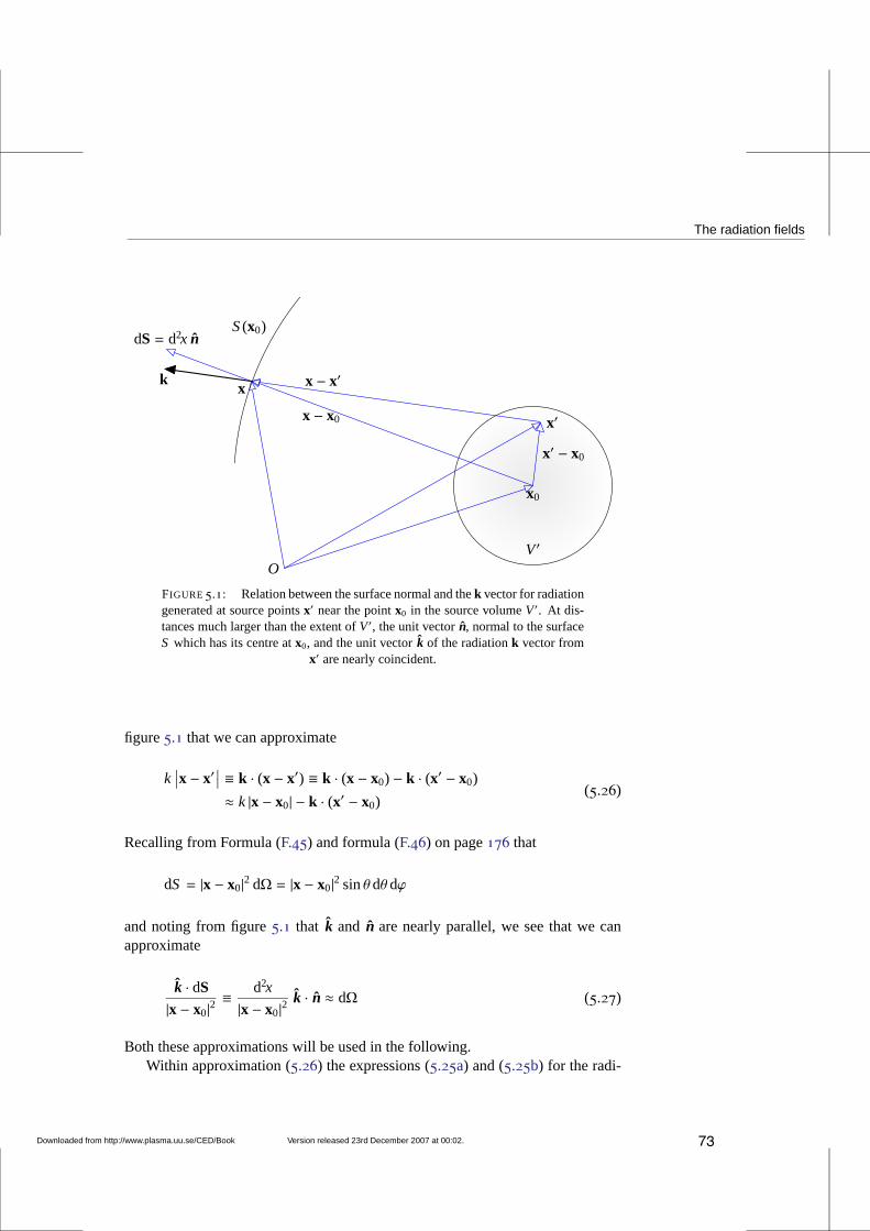
The radiation fields
V′
O
x0
x
x − x0
dS= d2x n
x′
x − x′
S(x0)
k
x′ − x0
FIGURE5.1: Relation between the surface normal and thek vector for radiationgenerated at source pointsx′ near the pointx0 in the source volumeV′. At dis-tances much larger than the extent ofV′, the unit vectorn, normal to the surfaceS which has its centre atx0, and the unit vectork of the radiationk vector from
x′ are nearly coincident.
figure5.1 that we can approximate
k∣∣x − x′
∣∣ ≡ k · (x − x′) ≡ k · (x − x0) − k · (x′ − x0)
≈ k |x − x0| − k · (x′ − x0)(5.26)
Recalling from Formula (F.45) and formula (F.46) on page176 that
dS = |x − x0|2 dΩ = |x − x0|2 sinθ dθ dϕ
and noting from figure5.1 that k and n are nearly parallel, we see that we canapproximate
k · dS
|x − x0|2≡ d2x
|x − x0|2k · n ≈ dΩ (5.27)
Both these approximations will be used in the following.Within approximation (5.26) the expressions (5.25a) and (5.25b) for the radi-
Downloaded from http://www.plasma.uu.se/CED/Book Version released 23rd December 2007 at 00:02. 73
5. Electromagnetic Fields from Arbitrary Source Distributions
ation fields can be approximated as
Bradω (x) ≈ −i
µ0
4πeik|x−x0|
∫
V′d3x′
jω(x′) × k|x − x′| e−ik·(x′−x0)
≈ −iµ0
4πeik|x−x0|
|x − x0|
∫
V′d3x′ [jω(x′) × k] e−ik·(x′−x0)
(5.28a)
Eradω (x) ≈ −i
14πε0c
eik|x−x0|∫
V′d3x′
[jω(x′) × k] × (x − x′)
|x − x′|2e−ik·(x′−x0)
≈ i1
4πε0ceik|x−x0|
|x − x0|(x − x0)|x − x0|
×
∫
V′d3x′ [jω(x′) × k] e−ik·(x′−x0)
(5.28b)
I.e., if max |x′ − x0| ≪ |x − x′|, then the fields can be approximated assphericalwavesmultiplied by dimensional and angular factors, with integrals over points inthe source volume only.
5.4 Radiated energyLet us consider the energy that is carried in the radiation fieldsBrad, equation (5.25a),andErad, equation (5.25b) on page72. We have to treat signals with limited life-time and hence finite frequency bandwidth differently from monochromatic sig-nals.
5.4.1 Monochromatic signalsIf the source is strictly monochromatic, we can obtain the temporal average of theradiated powerP directly, simply by averaging over one period so that
〈S〉 = 〈E × H〉 = 12µ0
ReE × B∗ = 12µ0
Re
Eωe−iωt× (Bωe−iωt)∗
=1
2µ0Re
Eω × B∗ω e−iωteiωt=
12µ0
Re
Eω × B∗ω
(5.29)
Using the far-field approximations (5.28a) and (5.28b) and the fact that 1/c =√ε0µ0 andR0 =
√µ0/ε0 according to the definition (2.26) on page29, we obtain
〈S〉 = 132π2
R01
|x − x0|2
∣∣∣∣
∫
V′d3x′ (jω × k)e−ik·(x′−x0)
∣∣∣∣
2 x − x0
|x − x0|(5.30)
74 Version released 23rd December 2007 at 00:02. Downloaded from http://www.plasma.uu.se/CED/Book
Radiated energy
or, making use of (5.27) on page73,
dPdΩ=
132π2
R0
∣∣∣∣
∫
V′d3x′ (jω × k)e−ik·(x′−x0)
∣∣∣∣
2
(5.31)
which is the radiated power per unit solid angle.
5.4.2 Finite bandwidth signalsA signal with finite pulse width in time (t) domain has a certain spread in fre-quency (ω) domain. To calculate the total radiated energy we need to integrateover the whole bandwidth. The total energy transmitted through a unit area is thetime integral of the Poynting vector:
∫ ∞
−∞dt S(t) =
∫ ∞
−∞dt (E × H)
=
∫ ∞
−∞dω∫ ∞
−∞dω′
∫ ∞
−∞dt (Eω × Hω′) e−i(ω+ω′)t
(5.32)
If we carry out the temporal integration first and use the factthat∫ ∞
−∞dt e−i(ω+ω′)t = 2πδ(ω + ω′) (5.33)
equation (5.32) can be written [cf. Parseval’s identity]∫ ∞
−∞dt S(t) = 2π
∫ ∞
−∞dω (Eω × H−ω)
= 2π
(∫ ∞
0dω (Eω × H−ω) +
∫ 0
−∞dω (Eω × H−ω)
)
= 2π
(∫ ∞
0dω (Eω × H−ω) −
∫ −∞
0dω (Eω × H−ω)
)
= 2π
(∫ ∞
0dω (Eω × H−ω) +
∫ ∞
0dω (E−ω × Hω)
)
=2πµ0
∫ ∞
0dω (Eω × B−ω + E−ω × Bω)
=2πµ0
∫ ∞
0dω (Eω × B∗ω + E∗ω × Bω)
(5.34)
where the last step follows from physical requirement of real-valuedness ofEω
andBω. We insert the Fourier transforms of the field components which dominateat large distances,i.e., the radiation fields (5.25a) and (5.25b). The result, after
Downloaded from http://www.plasma.uu.se/CED/Book Version released 23rd December 2007 at 00:02. 75
5. Electromagnetic Fields from Arbitrary Source Distributions
integration over the areaS of a large sphere which encloses the source volumeV′,is
U =14π
õ0
ε0
∮
Sd2x n ·
∫ ∞
0dω
∣∣∣∣
∫
V′d3x′
jω × k|x − x′|e
ik|x−x′ |∣∣∣∣
2
k (5.35)
Inserting the approximations (5.26) and (5.27) into equation (5.35) above andalso introducing
U =∫ ∞
0dωUω (5.36)
and recalling the definition (2.26) on page29 for the vacuum resistanceR0 weobtain
dUω
dΩdω ≈ 1
4πR0
∣∣∣∣
∫
V′d3x′ (jω × k)e−ik·(x′−x0)
∣∣∣∣
2
dω (5.37)
which, at large distances, is a good approximation to the energy that is radiatedper unit solid angle dΩ in a frequency band dω. It is important to notice thatFormula (5.37) includes only source coordinates. This means that the amount ofenergy that is being radiated is independent on the distanceto the source (as longas it is large).
5.5 Bibliography[1] F. HOYLE, SIR AND J. V. NARLIKAR , Lectures on Cosmology and Action at a Distance
Electrodynamics, World Scientific Publishing Co. Pte. Ltd, Singapore, New Jersey, Lon-don and Hong Kong, 1996, ISBN 9810-02-2573-3(pbk).46
[2] J. D. JACKSON, Classical Electrodynamics, third ed., John Wiley & Sons, Inc.,New York, NY . . . , 1999, ISBN 0-471-30932-X.
[3] L. D. LANDAU AND E. M. LIFSHITZ, The Classical Theory of Fields, fourth revised En-glish ed., vol. 2 ofCourse of Theoretical Physics, Pergamon Press, Ltd., Oxford . . . , 1975,ISBN 0-08-025072-6.
[4] W. K. H. PANOFSKY AND M. PHILLIPS, Classical Electricity and Magnetism, second ed.,Addison-Wesley Publishing Company, Inc., Reading, MA . . . ,1962, ISBN 0-201-05702-6.
[5] J. A. STRATTON, Electromagnetic Theory, McGraw-Hill Book Company, Inc., NewYork, NY and London, 1953, ISBN 07-062150-0.
76 Version released 23rd December 2007 at 00:02. Downloaded from http://www.plasma.uu.se/CED/Book
Downloaded from http://www.plasma.uu.se/CED/Book Version released 23rd December 2007 at 00:02.
6ELECTROMAGNETIC RADIATION
AND RADIATING SYSTEMS
In chapter3 we were able to derive general expressions for the scalar andvectorpotentials from which we then, in chapter5, calculated the total electric and mag-netic fields from arbitrary distributions of charge and current sources. The onlylimitation in the calculation of the fields was that the advanced potentials werediscarded.
Thus, one can, at least in principle, calculate the radiatedfields, Poyntingflux, energy and other electromagnetic quantities for an arbitrary current densityFourier component and then add these Fourier components together to constructthe complete electromagnetic field at any time at any point inspace. However, inpractice, it is often difficult to evaluate the source integrals unless the current hasa simple distribution in space. In the general case, one has to resort to approxima-tions. We shall consider both these situations.
6.1 Radiation from an extended source volume at restCertain radiating systems have a symmetric geometry or are in any other waysimple enough that a direct (semi-)analytic calculation ofthe radiated fields andenergy is possible. This is for instance the case when the radiating current flowsin a finite, conducting medium of simple geometry at rest suchas in a stationaryantenna.
77
6. Electromagnetic Radiation and Radiating Systems
6.1.1 Radiation from a one-dimensional current distributionLet us apply equation (5.31) on page75 to calculate the radiated EM power froma one-dimensional, time-varying current. Such a current can be set up by feedingthe EMF of a generator (eg., a transmitter) onto a stationary, linear, straight, thin,conducting wire across a very short gap at its centre. Due to the EMF the chargesin this thin wire of finite lengthL are set into motion to produce a time-varyingantenna currentwhich is the source of the EM radiation. Linear antennas of thistype are calleddipole antennas. For simplicity, we assume that the conductorresistance and the energy loss due to the electromagnetic radiation are negligible.
Choosing our coordinate system such that thex3 axis is along the antenna axis,the antenna current can be represented asj (t′, x′) = δ(x′1)δ(x
′2)J(t′, x′3) x3 (mea-
sured in A/m2) whereJ(t′, x′3) is the current (measured in A) along the antennawire. Since we can assume that the antenna wire is infinitely thin, the current mustvanish at the endpoints−L/2 andL/2 and is equal to the supplied current at themidpoint where the antenna is fed across a very short gap in the antenna wire.
For each Fourier frequency componentω0, the antenna currentJ(t′, x′3) can bewritten asI (x′3) exp−iω0t′ so that the antenna current density can be representedasj (t′, x′) = j0(x′) exp−iω0t′ [cf. equations (5.6) on page66] where
j0(x′) = δ(x′1)δ(x′2)I (x′3) (6.1)
and where the spatially varying Fourier amplitudeI (x′3) of the antenna currentfulfils the time-independent wave equation (Helmholtz equation)
d2I
dx′23+ k2I (x′3) = 0 , I (−L/2) = I (L/2) = 0 , I (0) = I0 (6.2)
This equation has the well-known solution
I (x′3) = I0sin[k(L/2−
∣∣x′3∣∣)]
sin(kL/2)(6.3)
whereI0 is the amplitude of the antenna current (measured in A), assumed to beconstant and supplied by the generator/transmitter at theantenna feed point(in ourcase the midpoint of the antenna wire) and 1/ sin(kL/2) is a normalisation factor.The antenna current forms astanding waveas indicated in figure6.1 on page79.
When the antenna is short we can approximate the current distribution for-mula (6.3) by the first term in its Taylor expansion,i.e., by I0(1 − 2|x′3|/L). Fora half-wave antenna (L = λ/2 ⇔ kL = π) formula (6.3) above simplifies toI0 cos(kx′3). Hence, in the most general case of a straight, infinitely thin antennaof finite, arbitrary lengthL directed along thex′3 axis, the Fourier amplitude of the
78 Version released 23rd December 2007 at 00:02. Downloaded from http://www.plasma.uu.se/CED/Book
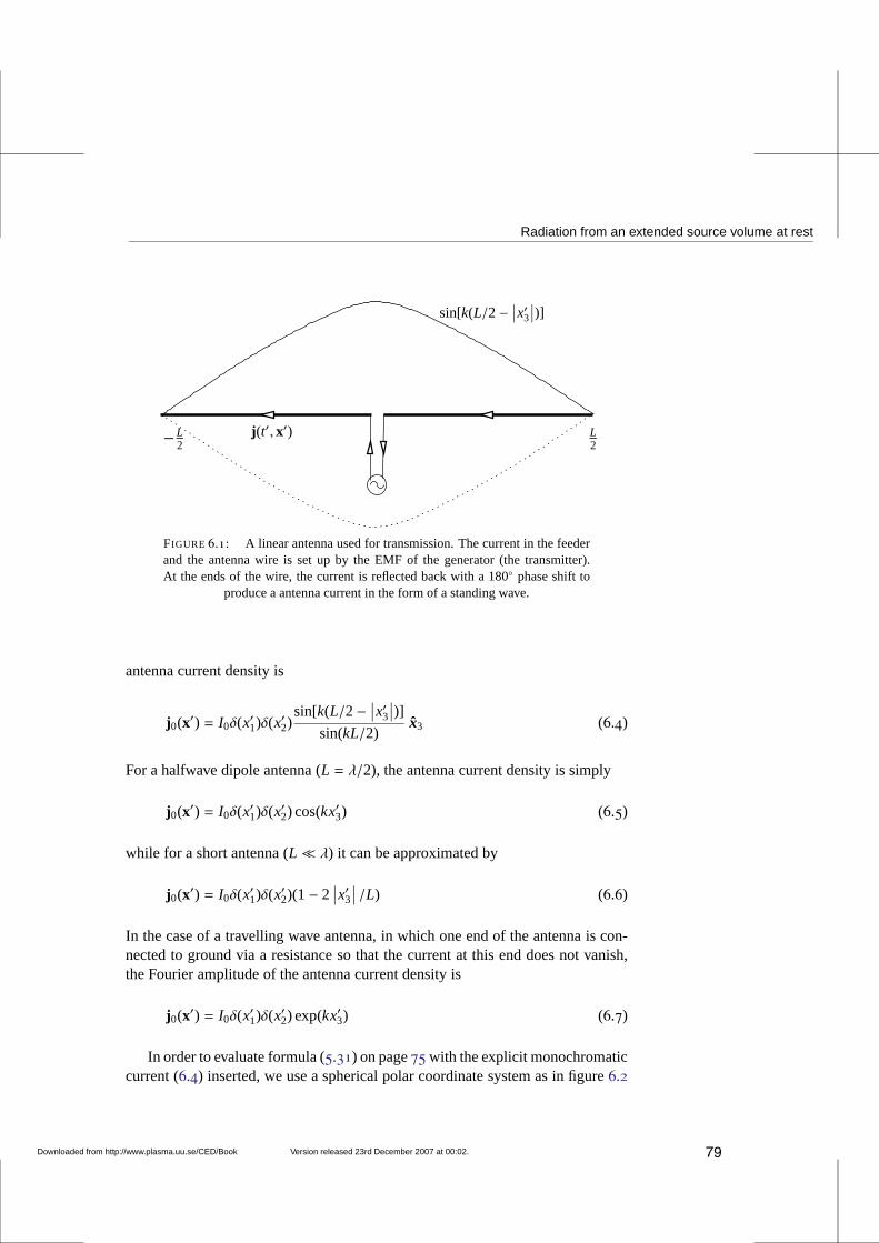
Radiation from an extended source volume at rest
j (t′, x′)− L2
sin[k(L/2−∣∣x′3∣∣)]
L2
FIGURE 6.1: A linear antenna used for transmission. The current in the feederand the antenna wire is set up by the EMF of the generator (the transmitter).At the ends of the wire, the current is reflected back with a 180 phase shift to
produce a antenna current in the form of a standing wave.
antenna current density is
j0(x′) = I0δ(x′1)δ(x′2)
sin[k(L/2−∣∣x′3∣∣)]
sin(kL/2)x3 (6.4)
For a halfwave dipole antenna (L = λ/2), the antenna current density is simply
j0(x′) = I0δ(x′1)δ(x′2) cos(kx′3) (6.5)
while for a short antenna (L ≪ λ) it can be approximated by
j0(x′) = I0δ(x′1)δ(x′2)(1− 2
∣∣x′3∣∣ /L) (6.6)
In the case of a travelling wave antenna, in which one end of the antenna is con-nected to ground via a resistance so that the current at this end does not vanish,the Fourier amplitude of the antenna current density is
j0(x′) = I0δ(x′1)δ(x′2) exp(kx′3) (6.7)
In order to evaluate formula (5.31) on page75with the explicit monochromaticcurrent (6.4) inserted, we use a spherical polar coordinate system as in figure6.2
Downloaded from http://www.plasma.uu.se/CED/Book Version released 23rd December 2007 at 00:02. 79
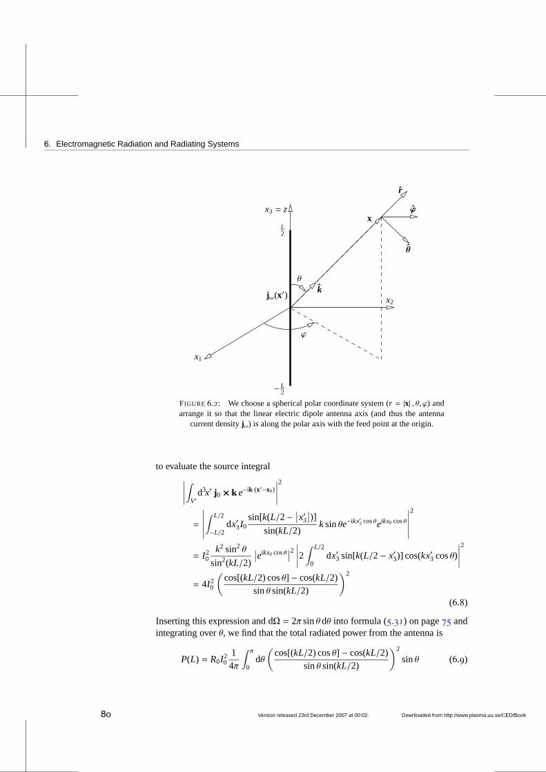
6. Electromagnetic Radiation and Radiating Systems
x3 = z
x2
x
jω(x′)
ϕ
k
x1
θ
r
θ
ϕ
L2
− L2
FIGURE 6.2: We choose a spherical polar coordinate system (r = |x| , θ, ϕ) andarrange it so that the linear electric dipole antenna axis (and thus the antenna
current densityjω) is along the polar axis with the feed point at the origin.
to evaluate the source integral∣∣∣∣
∫
V′d3x′ j0 × k e−ik·(x′−x0)
∣∣∣∣
2
=
∣∣∣∣∣
∫ L/2
−L/2dx′3I0
sin[k(L/2−∣∣x′3∣∣)]
sin(kL/2)ksinθe−ikx′3 cosθeikx0 cosθ
∣∣∣∣∣
2
= I20
k2 sin2 θ
sin2(kL/2)
∣∣eikx0 cosθ
∣∣2∣∣∣∣2∫ L/2
0dx′3 sin[k(L/2− x′3)] cos(kx′3 cosθ)
∣∣∣∣
2
= 4I20
(cos[(kL/2) cosθ] − cos(kL/2)
sinθ sin(kL/2)
)2
(6.8)
Inserting this expression and dΩ = 2π sinθ dθ into formula (5.31) on page75 andintegrating overθ, we find that the total radiated power from the antenna is
P(L) = R0I20
14π
∫ π
0dθ
(cos[(kL/2) cosθ] − cos(kL/2)
sinθ sin(kL/2)
)2
sinθ (6.9)
80 Version released 23rd December 2007 at 00:02. Downloaded from http://www.plasma.uu.se/CED/Book
Radiation from an extended source volume at rest
One can show that
limkL→0
P(L) =π
12
(Lλ
)2
R0I20 (6.10)
whereλ is the vacuum wavelength.The quantity
Rrad(L) =P(L)I2eff
=P(L)12 I2
0
= R0π
6
(Lλ
)2
≈ 197
(Lλ
)2
Ω (6.11)
is called theradiation resistance. For the technologically important case of ahalf-wave antenna,i.e., for L = λ/2 or kL = π, formula (6.9) on page80 reducesto
P(λ/2) = R0I20
14π
∫ π
0dθ
cos2(π2 cosθ
)
sinθ(6.12)
The integral in (6.12) can always be evaluated numerically. But, it can in fact alsobe evaluated analytically as follows:
∫ π
0
cos2(π2 cosθ
)
sinθdθ = [cosθ → u] =
∫ 1
−1
cos2(π2u)
1− u2du =
[
cos2(π
2u)
=1+ cos(πu)
2
]
=12
∫ 1
−1
1+ cos(πu)(1+ u)(1− u)
du
=14
∫ 1
−1
1+ cos(πu)(1+ u)
du+14
∫ 1
−1
1+ cos(πu)(1− u)
du
=12
∫ 1
−1
1+ cos(πu)(1+ u)
du =[
1+ u→ v
π
]
=12
∫ 2π
0
1− cosvv
dv =12
[γ + ln 2π − Ci(2π)]
≈ 1.22(6.13)
where in the last step theEuler-Mascheroni constantγ = 0.5772. . . and thecosineintegral Ci(x) were introduced. Inserting this into the expression equation (6.12)we obtain the valueRrad(λ/2) ≈ 73Ω.
6.1.2 Radiation from a two-dimensional current distributionAs an example of a two-dimensional current distribution we consider a circularloop antennaand calculate the radiated fields from such an antenna. We choose
Downloaded from http://www.plasma.uu.se/CED/Book Version released 23rd December 2007 at 00:02. 81
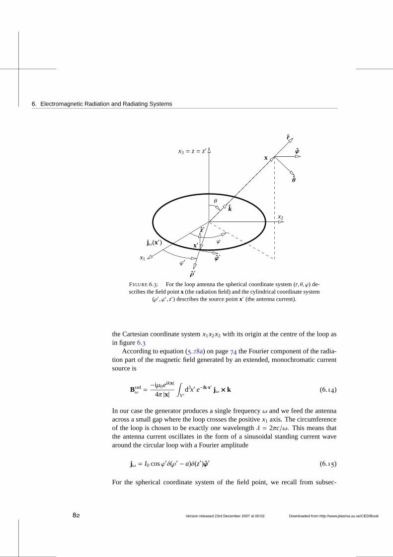
6. Electromagnetic Radiation and Radiating Systems
x2
k
ϕ
ϕ′
jω(x′)
x1
x′
ρ′
ϕ′
θ
θ
ϕx
r
x3 = z= z′
z′
FIGURE 6.3: For the loop antenna the spherical coordinate system (r, θ, ϕ) de-scribes the field pointx (the radiation field) and the cylindrical coordinate system
(ρ′, ϕ′, z′) describes the source pointx′ (the antenna current).
the Cartesian coordinate systemx1x2x3 with its origin at the centre of the loop asin figure6.3
According to equation (5.28a) on page74 the Fourier component of the radia-tion part of the magnetic field generated by an extended, monochromatic currentsource is
Bradω =
−iµ0eik|x|
4π |x|
∫
V′d3x′ e−ik·x′ jω × k (6.14)
In our case the generator produces a single frequencyω and we feed the antennaacross a small gap where the loop crosses the positivex1 axis. The circumferenceof the loop is chosen to be exactly one wavelengthλ = 2πc/ω. This means thatthe antenna current oscillates in the form of a sinusoidal standing current wavearound the circular loop with a Fourier amplitude
jω = I0 cosϕ′δ(ρ′ − a)δ(z′)ϕ′ (6.15)
For the spherical coordinate system of the field point, we recall from subsec-
82 Version released 23rd December 2007 at 00:02. Downloaded from http://www.plasma.uu.se/CED/Book
Radiation from an extended source volume at rest
tion F.4.1 on page176 that the following relations between the base vectors hold:
r = sinθ cosϕx1 + sinθ sinϕx2 + cosθx3
θ = cosθ cosϕx1 + cosθ sinϕx2 − sinθx3
ϕ = − sinϕx1 + cosϕx2
and
x1 = sinθ cosϕr + cosθ cosϕθ − sinϕϕ
x2 = sinθ sinϕr + cosθ sinϕθ + cosϕϕ
x3 = cosθ r − sinθθ
With the use of the above transformations and trigonometricidentities, we obtainfor the cylindrical coordinate system which describes the source:
ρ′ = cosϕ′ x1 + sinϕ′ x2
= sinθ cos(ϕ′ − ϕ)r + cosθ cos(ϕ′ − ϕ)θ + sin(ϕ′ − ϕ)ϕ(6.16)
ϕ′ = − sinϕ′ x1 + cosϕ′ x2
= − sinθ sin(ϕ′ − ϕ)r − cosθ sin(ϕ′ − ϕ)θ + cos(ϕ′ − ϕ)ϕ(6.17)
z′ = x3 = cosθ r − sinθθ (6.18)
This choice of coordinate systems means thatk = kr andx′ = aρ′ so that
k · x′ = kasinθ cos(ϕ′ − ϕ) (6.19)
and
ϕ′ × k = k[cos(ϕ′ − ϕ)θ + cosθ sin(ϕ′ − ϕ)ϕ] (6.20)
With these expressions inserted, recalling that in cylindrical coordinates d3x′ =ρ′dρ′dϕ′dz′, the source integral becomes
∫
V′d3x′ e−ik·x′ jω × k = a
∫ 2π
0dϕ′ e−ikasinθ cos(ϕ′−ϕ)I0 cosϕ′ ϕ′ × k
= I0ak∫ 2π
0e−ikasinθ cos(ϕ′−ϕ) cos(ϕ′ − ϕ) cosϕ′ dϕ′ θ
+ I0ak cosθ∫ 2π
0e−ikasinθ cos(ϕ′−ϕ) sin(ϕ′ − ϕ) cosϕ′ dϕ′ ϕ
(6.21)
Utilising the periodicity of the integrands over the integration interval [0, 2π],introducing the auxiliary integration variableϕ′′ = ϕ′ − ϕ, and utilising standard
Downloaded from http://www.plasma.uu.se/CED/Book Version released 23rd December 2007 at 00:02. 83
6. Electromagnetic Radiation and Radiating Systems
trigonometric identities, the first integral in the RHS of (6.21) can be rewritten∫ 2π
0e−ikasinθ cosϕ′′ cosϕ′′ cos(ϕ′′ + ϕ) dϕ′′
= cosϕ∫ 2π
0e−ikasinθ cosϕ′′ cos2 ϕ′′ dϕ′′ + a vanishing integral
= cosϕ∫ 2π
0e−ikasinθ cosϕ′′
(12+
12
cos 2ϕ′′)
dϕ′′
=12
cosϕ∫ 2π
0e−ikasinθ cosϕ′′ dϕ′′
+12
cosϕ∫ 2π
0e−ikasinθ cosϕ′′ cos(2ϕ′′) dϕ′′
(6.22)
Analogously, the second integral in the RHS of (6.21) can be rewritten∫ 2π
0e−ikasinθ cosϕ′′ sinϕ′′ cos(ϕ′′ + ϕ) dϕ′′
=12
sinϕ∫ 2π
0e−ikasinθ cosϕ′′ dϕ′′
− 12
sinϕ∫ 2π
0e−ikasinθ cosϕ′′ cos 2ϕ′′ dϕ′′
(6.23)
As is well-known from the theory ofBessel functions,
Jn(−ξ) = (−1)nJn(ξ)
Jn(−ξ) =i−n
π
∫ π
0e−iξ cosϕ cosnϕdϕ =
i−n
2π
∫ 2π
0e−iξ cosϕ cosnϕdϕ
(6.24)
which means that∫ 2π
0e−ikasinθ cosϕ′′ dϕ′′ = 2πJ0(kasinθ)
∫ 2π
0e−ikasinθ cosϕ′′ cos 2ϕ′′ dϕ′′ = −2πJ2(kasinθ)
(6.25)
Putting everything together, we find that∫
V′d3x′ e−ik·x′ jω × k = Iθ θ + Iϕ ϕ
= I0akπ cosϕ [J0(kasinθ) − J2(kasinθ)] θ
+ I0akπ cosθ sinϕ [J0(kasinθ) + J2(kasinθ)] ϕ
(6.26)
so that, in spherical coordinates where|x| = r,
Bradω (x) =
−iµ0eikr
4πr
(Iθ θ + Iϕ ϕ
)(6.27)
84 Version released 23rd December 2007 at 00:02. Downloaded from http://www.plasma.uu.se/CED/Book
Radiation from a localised source volume at rest
To obtain the desired physical magnetic field in the radiation (far) zone wemust Fourier transform back tot space and take the real part and evaluate it at theretarded time:
Brad(t, x) = Re
−iµ0e(ikr−ωt′)
4πr
(Iθ θ + Iϕ ϕ
)
=µ0
4πrsin(kr − ωt′)
(Iθ θ + Iϕ ϕ
)
=I0akµ0
4rsin(kr − ωt′)
(
cosϕ [J0(kasinθ) − J2(kasinθ)] θ
+ cosθ sinϕ [J0(kasinθ) + J2(kasinθ)] ϕ
)
(6.28)
From this expression for the radiatedB field, we can obtain the radiatedE fieldwith the help of Maxwell’s equations.
6.2 Radiation from a localised source volume at restIn the general case, and when we are interested in evaluatingthe radiation far froma source at rest and which is localised in a small volume, we can introduce anapproximation which leads to amultipole expansionwhere individual terms canbe evaluated analytically. We shall usethe Hertz methodto obtain this expansion.
6.2.1 The Hertz potentialIn section4.1.1 we introduced the electric polarisationP(t, x) such that the polari-sation charge densityρpol = −∇ ·P. If we adopt the same idea for the ‘true’ chargedensity and introduce a vector fieldπ(t, x) such that
ρtrue = −∇ · π (6.29a)
which means that the associated ‘polarisation current’ becomes
∂π
∂t= j true (6.29b)
As a consequence, the equation of continuity for ‘true’ charges and currents [cf.expression (1.23) on page10] is satisfied:
∂ρtrue(t, x)∂t
+ ∇ · j true(t, x) = − ∂∂t∇ · π + ∇ · ∂π
∂t= 0 (6.30)
Downloaded from http://www.plasma.uu.se/CED/Book Version released 23rd December 2007 at 00:02. 85
6. Electromagnetic Radiation and Radiating Systems
Furthermore, if we compare with the electric polarisation [cf. equation (4.9) onpage55], we see that the quantityπ is indeed related to the ‘true’ charges in thesame way asP is related to polarised charge, namely as a dipole moment density.The quantityπ is referred to as thepolarisation vectorsince, formally, it treatsalso the ‘true’ (free) charges as polarisation charges so that
∇ · E = ρtrue+ ρpol
ε0=−∇ · π − ∇ · P
ε0(6.31)
We introduce a further potentialΠe with the following property
∇ ·Πe = −φ (6.32a)
1c2
∂Πe
∂t= A (6.32b)
whereφ andA are the electromagnetic scalar and vector potentials, respectively.As we see,Πe acts as a ‘super-potential’ in the sense that it is a potential fromwhich we can obtain other potentials. It is called theHertz vectoror polarisationpotential. Requiring that the scalar and vector potentialsφ andA, respectively,fulfil their inhomogeneous wave equations, equations (3.14) on page43, one finds,using (6.29) and (6.32), that the Hertz vector must satisfy the inhomogeneouswave equation
2Π
e =1c2
∂2
∂t2Π
e− ∇2Π
e =π
ε0(6.33)
This equation is of the same type as equation (3.17) on page43, and has there-fore the retarded solution
Πe(t, x) =
14πε0
∫
V′d3x′π(t′ret, x
′)|x − x′| (6.34)
with Fourier components
Πeω(x) =
14πε0
∫
V′d3x′πω(x′)eik|x−x′ |
|x − x′| (6.35)
If we introduce thehelp vectorC such that
C = ∇ ×Πe (6.36)
we see that we can calculate the magnetic and electric fields,respectively, as fol-lows
B =1c2
∂C∂t
(6.37a)
E = ∇ × C (6.37b)
86 Version released 23rd December 2007 at 00:02. Downloaded from http://www.plasma.uu.se/CED/Book
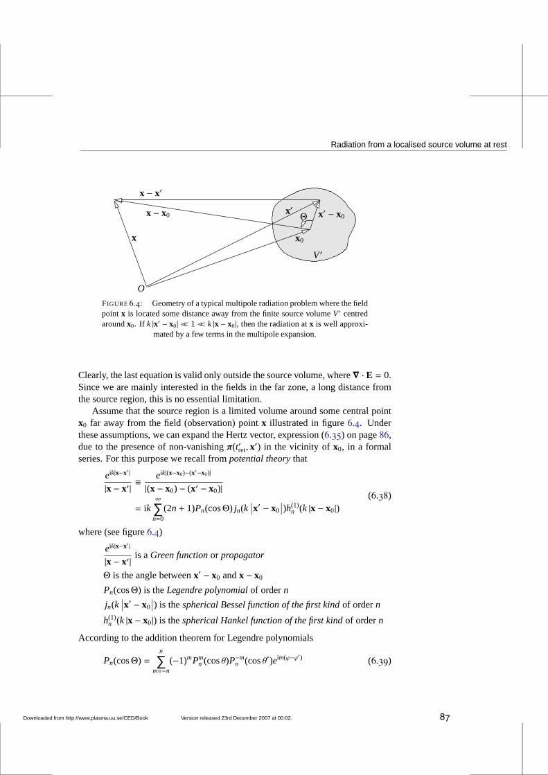
Radiation from a localised source volume at rest
x
x − x0
x0
V′
O
Θx′
x − x′
x′ − x0
FIGURE6.4: Geometry of a typical multipole radiation problem where thefieldpoint x is located some distance away from the finite source volumeV′ centredaroundx0. If k |x′ − x0| ≪ 1≪ k |x − x0|, then the radiation atx is well approxi-
mated by a few terms in the multipole expansion.
Clearly, the last equation is valid only outside the source volume, where∇ · E = 0.Since we are mainly interested in the fields in the far zone, a long distance fromthe source region, this is no essential limitation.
Assume that the source region is a limited volume around somecentral pointx0 far away from the field (observation) pointx illustrated in figure6.4. Underthese assumptions, we can expand the Hertz vector, expression (6.35) on page86,due to the presence of non-vanishingπ(t′ret, x
′) in the vicinity of x0, in a formalseries. For this purpose we recall frompotential theorythat
eik|x−x′ |
|x − x′| ≡eik|(x−x0)−(x′−x0)|
|(x − x0) − (x′ − x0)|
= ik∞
∑n=0
(2n+ 1)Pn(cosΘ) jn(k∣∣x′ − x0
∣∣)h(1)
n (k |x − x0|)(6.38)
where (see figure6.4)
eik|x−x′ |
|x − x′| is aGreen functionor propagator
Θ is the angle betweenx′ − x0 andx − x0
Pn(cosΘ) is theLegendre polynomialof ordern
jn(k∣∣x′ − x0
∣∣) is thespherical Bessel function of the first kindof ordern
h(1)n (k |x − x0|) is thespherical Hankel function of the first kindof ordern
According to the addition theorem for Legendre polynomials
Pn(cosΘ) =n
∑m=−n
(−1)mPmn (cosθ)P−m
n (cosθ′)eim(ϕ−ϕ′) (6.39)
Downloaded from http://www.plasma.uu.se/CED/Book Version released 23rd December 2007 at 00:02. 87
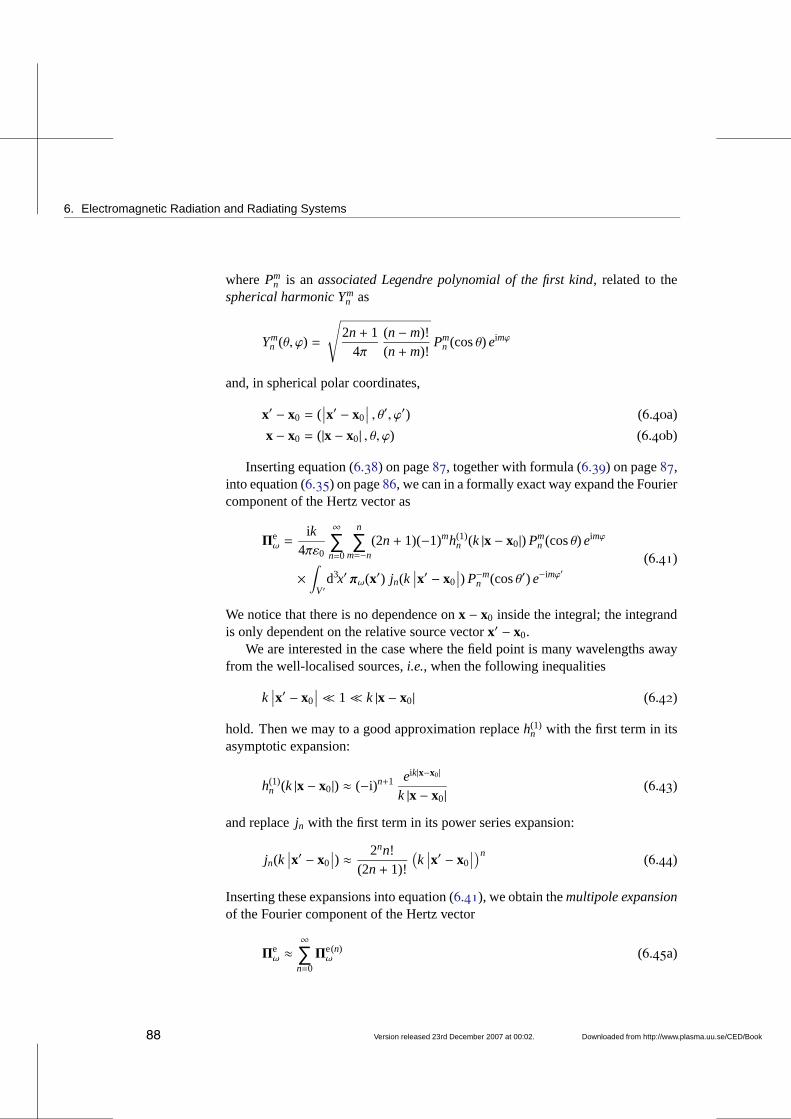
6. Electromagnetic Radiation and Radiating Systems
wherePmn is anassociated Legendre polynomial of the first kind, related to the
spherical harmonic Ymn as
Ymn (θ, ϕ) =
√
2n+ 14π
(n−m)!(n+m)!
Pmn (cosθ) eimϕ
and, in spherical polar coordinates,
x′ − x0 = (∣∣x′ − x0
∣∣ , θ′, ϕ′) (6.40a)
x − x0 = (|x − x0| , θ, ϕ) (6.40b)
Inserting equation (6.38) on page87, together with formula (6.39) on page87,into equation (6.35) on page86, we can in a formally exact way expand the Fouriercomponent of the Hertz vector as
Πeω =
ik4πε0
∞
∑n=0
n
∑m=−n
(2n+ 1)(−1)mh(1)n (k |x − x0|) Pm
n (cosθ) eimϕ
×∫
V′d3x′ πω(x′) jn(k
∣∣x′ − x0
∣∣) P−m
n (cosθ′) e−imϕ′(6.41)
We notice that there is no dependence onx − x0 inside the integral; the integrandis only dependent on the relative source vectorx′ − x0.
We are interested in the case where the field point is many wavelengths awayfrom the well-localised sources,i.e., when the following inequalities
k∣∣x′ − x0
∣∣≪ 1≪ k |x − x0| (6.42)
hold. Then we may to a good approximation replaceh(1)n with the first term in its
asymptotic expansion:
h(1)n (k |x − x0|) ≈ (−i)n+1 eik|x−x0|
k |x − x0|(6.43)
and replacejn with the first term in its power series expansion:
jn(k∣∣x′ − x0
∣∣) ≈ 2nn!
(2n+ 1)!
(k∣∣x′ − x0
∣∣)n
(6.44)
Inserting these expansions into equation (6.41), we obtain themultipole expansionof the Fourier component of the Hertz vector
Πeω ≈
∞
∑n=0
Πeω(n) (6.45a)
88 Version released 23rd December 2007 at 00:02. Downloaded from http://www.plasma.uu.se/CED/Book
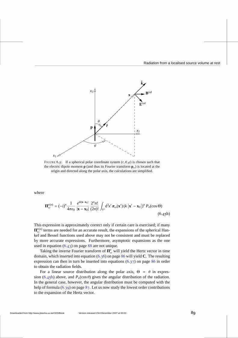
Radiation from a localised source volume at rest
Erad
x2
ϕ
r
x
k
Bradx3
p
x1
θ
FIGURE 6.5: If a spherical polar coordinate system (r, θ, ϕ) is chosen such thatthe electric dipole momentp (and thus its Fourier transformpω) is located at the
origin and directed along the polar axis, the calculations are simplified.
where
Πeω(n) = (−i)n 1
4πε0
eik|x−x0|
|x − x0|2nn!(2n)!
∫
V′d3x′ πω(x′) (k
∣∣x′ − x0
∣∣)n Pn(cosΘ)
(6.45b)
This expression is approximately correct only if certain care is exercised; if manyΠ
eω(n) terms are needed for an accurate result, the expansions of the spherical Han-
kel and Bessel functions used above may not be consistent andmust be replacedby more accurate expressions. Furthermore, asymptotic expansions as the oneused in equation (6.43) on page88 are not unique.
Taking the inverse Fourier transform ofΠeω will yield the Hertz vector in time
domain, which inserted into equation (6.36) on page86will yield C. The resultingexpression can then in turn be inserted into equations (6.37) on page86 in orderto obtain the radiation fields.
For a linear source distribution along the polar axis,Θ = θ in expres-sion (6.45b) above, andPn(cosθ) gives the angular distribution of the radiation.In the general case, however, the angular distribution mustbe computed with thehelp of formula (6.39) on page87. Let us now study the lowest order contributionsto the expansion of the Hertz vector.
Downloaded from http://www.plasma.uu.se/CED/Book Version released 23rd December 2007 at 00:02. 89
6. Electromagnetic Radiation and Radiating Systems
6.2.2 Electric dipole radiationChoosingn = 0 in expression (6.45b) on page89, we obtain
Πeω(0) =
eik|x−x0|
4πε0 |x − x0|
∫
V′d3x′ πω(x′) =
14πε0
eik|x−x0|
|x − x0|pω (6.46)
Sinceπ represents a dipole moment density for the ‘true’ charges (in the samevein asP does so for the polarised charges),pω =
∫
V′d3x′ πω(x′) is, by definition,
the Fourier component of theelectric dipole moment
p(t, x0) =∫
V′d3x′ π(t′, x′) =
∫
V′d3x′ (x′ − x0)ρ(t′, x′) (6.47)
[cf. equation (4.2) on page54 which describes the static dipole moment]. Ifa spherical coordinate system is chosen with its polar axis along pω as in fig-ure6.5 on page89, the components ofΠe
ω(0) are
Πer
def≡ Πeω(0) · r = 1
4πε0
eik|x−x0|
|x − x0|pω cosθ (6.48a)
Πeθ
def≡ Πeω(0) · θ = − 1
4πε0
eik|x−x0|
|x − x0|pω sinθ (6.48b)
Πeϕ
def≡ Πeω(0) · ϕ = 0 (6.48c)
Evaluating formula (6.36) on page86 for the help vectorC, with the spheri-cally polar components (6.48) of Πe
ω(0) inserted, we obtain
Cω = C(0)ω,ϕ ϕ =
14πε0
(1
|x − x0|− ik
)eik|x−x0|
|x − x0|pω sinθ ϕ (6.49)
Applying this to equations (6.37) on page86, we obtain directly the Fourier com-ponents of the fields
Bω = −iωµ0
4π
(1
|x − x0|− ik
)eik|x−x0|
|x − x0|pω sinθ ϕ (6.50a)
Eω =1
4πε0
[
2
(1
|x − x0|2− ik|x − x0|
)
cosθx − x0
|x − x0|
+
(1
|x − x0|2− ik|x − x0|
− k2
)
sinθ θ
]eik|x−x0|
|x − x0|pω
(6.50b)
Keeping only those parts of the fields which dominate at largedistances (theradiation fields) and recalling that the wave vectork = k(x − x0)/ |x − x0| where
90 Version released 23rd December 2007 at 00:02. Downloaded from http://www.plasma.uu.se/CED/Book
Radiation from a localised source volume at rest
k = ω/c, we can now write down the Fourier components of the radiation parts ofthe magnetic and electric fields from the dipole:
Bradω = −
ωµ0
4πeik|x−x0|
|x − x0|pωksinθ ϕ = −ωµ0
4πeik|x−x0|
|x − x0|(pω × k) (6.51a)
Eradω = −
14πε0
eik|x−x0|
|x − x0|pωk2 sinθ θ = − 1
4πε0
eik|x−x0|
|x − x0|[(pω × k) × k] (6.51b)
These fields constitute theelectric dipole radiation, also known asE1 radiation.
6.2.3 Magnetic dipole radiationThe next term in the expression (6.45b) on page89 for the expansion of the Fouriertransform of the Hertz vector is forn = 1:
Πeω(1) = −i
eik|x−x0|
4πε0 |x − x0|
∫
V′d3x′ k
∣∣x′ − x0
∣∣πω(x′) cosΘ
= −ik1
4πε0
eik|x−x0|
|x − x0|2∫
V′d3x′ [(x − x0) · (x′ − x0)] πω(x′)
(6.52)
Here, the term [(x − x0) · (x′ − x0)] πω(x′) can be rewritten
[(x − x0) · (x′ − x0)] πω(x′) = (xi − x0,i)(x′i − x0,i)πω(x′) (6.53)
and introducing
ηi = xi − x0,i (6.54a)
η′i = x′i − x0,i (6.54b)
the jth component of the integrand inΠeω
(1) can be broken up into
[(x − x0) · (x′ − x0)] πω(x′) j =12ηi
(πω, jη
′i + πω,iη
′j
)
+12ηi
(πω, jη
′i − πω,iη′j
)(6.55)
i.e., as the sum of two parts, the first being symmetric and the second antisymmet-ric in the indicesi, j. We note that the antisymmetric part can be written as
12ηi
(πω, jη
′i − πω,iη′j
)=
12
[πω, j(ηiη′i ) − η′j(ηiπω,i)]
=12
[πω(η · η′) − η′(η · πω)] j
=12
(x − x0) × [πω × (x′ − x0)]
j
(6.56)
Downloaded from http://www.plasma.uu.se/CED/Book Version released 23rd December 2007 at 00:02. 91
6. Electromagnetic Radiation and Radiating Systems
The utilisation of equations (6.29) on page85, and the fact that we are consid-ering a single Fourier component,
π(t, x) = πωe−iωt (6.57)
allow us to expressπω in jω as
πω = ijωω
(6.58)
Hence, we can write the antisymmetric part of the integral informula (6.52) onpage91 as
12
(x − x0) ×∫
V′d3x′ πω(x′) × (x′ − x0)
= i1
2ω(x − x0) ×
∫
V′d3x′ jω(x′) × (x′ − x0)
= −i1ω
(x − x0) ×mω
(6.59)
where we introduced the Fourier transform of themagnetic dipole moment
mω =12
∫
V′d3x′ (x′ − x0) × jω(x′) (6.60)
The final result is that the antisymmetric, magnetic dipole,part ofΠeω(1) can be
written
Πe,antisymω
(1)= − k
4πε0ω
eik|x−x0|
|x − x0|2(x − x0) ×mω (6.61)
In analogy with the electric dipole case, we insert this expression into equa-tion (6.36) on page86 to evaluateC, with which equations (6.37) on page86then gives theB andE fields. Discarding, as before, all terms belonging to thenear fields and transition fields and keeping only the terms that dominate at largedistances, we obtain
Bradω (x) = − µ0
4πeik|x−x0|
|x − x0|(mω × k) × k (6.62a)
Eradω (x) =
k4πε0c
eik|x−x0|
|x − x0|mω × k (6.62b)
which are the fields of themagnetic dipole radiation(M1 radiation).
92 Version released 23rd December 2007 at 00:02. Downloaded from http://www.plasma.uu.se/CED/Book
Radiation from a localised charge in arbitrary motion
6.2.4 Electric quadrupole radiation
The symmetric partΠe,symω
(1) of then = 1 contribution in the equation (6.45b) onpage89 for the expansion of the Hertz vector can be expressed in terms of theelectric quadrupole tensor, which is defined in accordance with equation (4.3) onpage54:
Q(t, x0) =∫
V′d3x′ (x′ − x0)(x′ − x0)ρ(t′ret, x
′) (6.63)
Again we use this expression in equation (6.36) on page86 to calculate the fieldsvia equations (6.37) on page86. Tedious, but fairly straightforward algebra (whichwe will not present here), yields the resulting fields. The radiation components ofthe fields in the far field zone (wave zone) are given by
Bradω (x) =
iµ0ω
8πeik|x−x0|
|x − x0|(k ·Qω) × k (6.64a)
Eradω (x) =
i8πε0
eik|x−x0|
|x − x0|[(k ·Qω) × k] × k (6.64b)
This type of radiation is calledelectric quadrupole radiationor E2 radiation.
6.3 Radiation from a localised charge in arbitrary mo-tionThe derivation of the radiation fields for the case of the source moving relativeto the observer is considerably more complicated than the stationary cases stud-ied above. In order to handle this non-stationary situation, we use the retardedpotentials (3.34) on page46 in chapter3
φ(t, x) =1
4πε0
∫
V′d3x′
ρ(t′ret, x
′(t′ret))
∣∣x(t) − x′(t′ret)
∣∣
(6.65a)
A(t, x) =µ0
4π
∫
V′d3x′
j(t′ret, x(t′ret)
)
∣∣x(t) − x′(t′ret)
∣∣
(6.65b)
and consider a source region with such a limited spatial extent that the chargesand currents are well localised. Specifically, we consider achargeq′, for instancean electron, which, classically, can be thought of as a localised, unstructured andrigid ‘charge distribution’ with a small, finite radius. Thepart of this ‘charge dis-tribution’ dq′ which we are considering is located in dV′ = d3x′ in the sphere in
Downloaded from http://www.plasma.uu.se/CED/Book Version released 23rd December 2007 at 00:02. 93
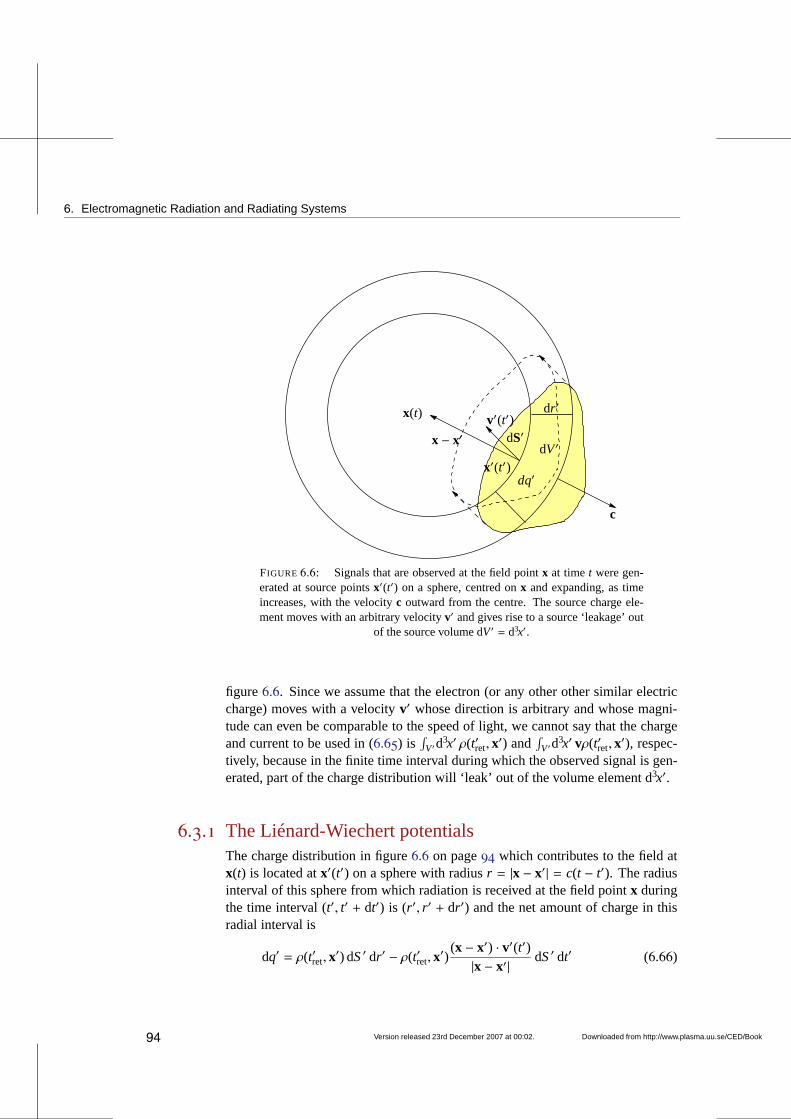
6. Electromagnetic Radiation and Radiating Systems
dq′
x(t)
x′(t′)dV′
dr ′
c
dS′x − x′v′(t′)
FIGURE 6.6: Signals that are observed at the field pointx at timet were gen-erated at source pointsx′(t′) on a sphere, centred onx and expanding, as timeincreases, with the velocityc outward from the centre. The source charge ele-ment moves with an arbitrary velocityv′ and gives rise to a source ‘leakage’ out
of the source volume dV′ = d3x′.
figure6.6. Since we assume that the electron (or any other other similar electriccharge) moves with a velocityv′ whose direction is arbitrary and whose magni-tude can even be comparable to the speed of light, we cannot say that the chargeand current to be used in (6.65) is
∫
V′d3x′ ρ(t′ret, x
′) and∫
V′d3x′ vρ(t′ret, x
′), respec-tively, because in the finite time interval during which the observed signal is gen-erated, part of the charge distribution will ‘leak’ out of the volume element d3x′.
6.3.1 The Liénard-Wiechert potentialsThe charge distribution in figure6.6 on page94 which contributes to the field atx(t) is located atx′(t′) on a sphere with radiusr = |x − x′| = c(t − t′). The radiusinterval of this sphere from which radiation is received at the field pointx duringthe time interval (t′, t′ + dt′) is (r ′, r ′ + dr ′) and the net amount of charge in thisradial interval is
dq′ = ρ(t′ret, x′) dS′ dr ′ − ρ(t′ret, x
′)(x − x′) · v′(t′)|x − x′| dS′ dt′ (6.66)
94 Version released 23rd December 2007 at 00:02. Downloaded from http://www.plasma.uu.se/CED/Book
Radiation from a localised charge in arbitrary motion
where the last term represents the amount of ‘source leakage’ due to the fact thatthe charge distribution moves with velocityv′(t′) = dx′/dt′. Since dt′ = dr ′/c anddS′ dr ′ = d3x′ we can rewrite the expression for the net charge as
dq′ = ρ(t′ret, x′) d3x′ − ρ(t′ret, x
′)(x − x′) · v′
c |x − x′| d3x′
= ρ(t′ret, x′)
(
1− (x − x′) · v′c |x − x′|
)
d3x′(6.67)
or
ρ(t′ret, x′) d3x′ =
dq′
1− (x−x′)·v′c|x−x′ |
(6.68)
which leads to the expression
ρ(t′ret, x′)
|x − x′| d3x′ =dq′
|x − x′| − (x−x′)·v′c
(6.69)
This is the expression to be used in the formulae (6.65) on page93 for the retardedpotentials. The result is (recall thatj = ρv)
φ(t, x) =1
4πε0
∫dq′
|x − x′| − (x−x′)·v′c
(6.70a)
A(t, x) =µ0
4π
∫v′ dq′
|x − x′| − (x−x′)·v′c
(6.70b)
For a sufficiently small and well localised charge distribution we can, assumingthat the integrands do not change sign in the integration volume, use the meanvalue theorem to evaluate these expressions to become
φ(t, x) =1
4πε0
1
|x − x′| − (x−x′)·v′c
∫
V′d3x′ dq′ =
q′
4πε0
1s
(6.71a)
A(t, x) =1
4πε0c2
v′
|x − x′| − (x−x′)·v′c
∫
V′d3x′ dq′ =
q′
4πε0c2
v′
s=
v′
c2φ(t, x)
(6.71b)
where
s= s(t′, x) =∣∣x − x′(t′)
∣∣ − [x − x′(t′)] · v′(t′)
c(6.72a)
=∣∣x − x′(t′)
∣∣
(
1− x − x′(t′)|x − x′(t′)| ·
v′(t′)c
)
(6.72b)
= [x − x′(t′)] ·(
x − x′(t′)|x − x′(t′)| −
v′(t′)c
)
(6.72c)
Downloaded from http://www.plasma.uu.se/CED/Book Version released 23rd December 2007 at 00:02. 95
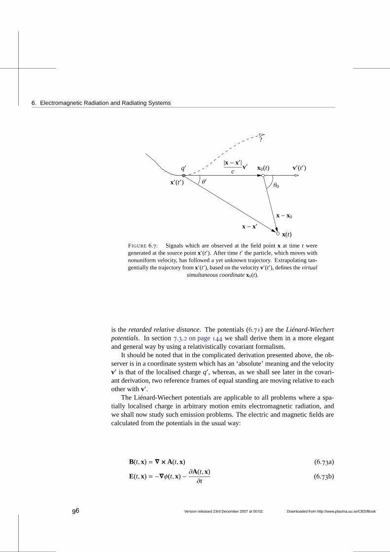
6. Electromagnetic Radiation and Radiating Systems
|x − x′|c
v′
x(t)
v′(t′)x0(t)
x′(t′)
x − x′x − x0
q′
θ′θ0
?
FIGURE 6.7: Signals which are observed at the field pointx at time t weregenerated at the source pointx′(t′). After time t′ the particle, which moves withnonuniform velocity, has followed a yet unknown trajectory. Extrapolating tan-gentially the trajectory fromx′(t′), based on the velocityv′(t′), defines thevirtual
simultaneous coordinatex0(t).
is theretarded relative distance. The potentials (6.71) are theLiénard-Wiechertpotentials. In section7.3.2 on page144 we shall derive them in a more elegantand general way by using a relativistically covariant formalism.
It should be noted that in the complicated derivation presented above, the ob-server is in a coordinate system which has an ‘absolute’ meaning and the velocityv′ is that of the localised chargeq′, whereas, as we shall see later in the covari-ant derivation, two reference frames of equal standing are moving relative to eachother withv′.
The Liénard-Wiechert potentials are applicable to all problems where a spa-tially localised charge in arbitrary motion emits electromagnetic radiation, andwe shall now study such emission problems. The electric and magnetic fields arecalculated from the potentials in the usual way:
B(t, x) = ∇ × A(t, x) (6.73a)
E(t, x) = −∇φ(t, x) − ∂A(t, x)∂t
(6.73b)
96 Version released 23rd December 2007 at 00:02. Downloaded from http://www.plasma.uu.se/CED/Book
Radiation from a localised charge in arbitrary motion
6.3.2 Radiation from an accelerated point chargeConsider a localised chargeq′ and assume that its trajectory is known experimen-tally as a function ofretarded time
x′ = x′(t′) (6.74)
(in the interest of simplifying our notation, we drop the subscript ‘ret’ on t′ fromnow on). This means that we know the trajectory of the chargeq′, i.e., x′, for alltimes up to the timet′ at which a signal was emitted in order to precisely arrive atthe field pointx at timet. Because of the finite speed of propagation of the fields,the trajectory at times later thant′ cannot be known at timet.
The retarded velocity and acceleration at timet′ are given by
v′(t′) =dx′
dt′(6.75a)
a′(t′) = v′(t′) =dv′
dt′=
d2x′
dt′2(6.75b)
As for the charge coordinatex′ itself, we have in general no knowledge of thevelocity and acceleration at times later thant′, and definitely not at the time ofobservationt! If we choose the field pointx as fixed, the application of (6.75) tothe relative vectorx − x′ yields
ddt′
[x − x′(t′)] = −v′(t′) (6.76a)
d2
dt′2[x − x′(t′)] = −v′(t′) (6.76b)
The retarded timet′ can, at least in principle, be calculated from the implicitrelation
t′ = t′(t, x) = t − |x − x′(t′)|c
(6.77)
and we shall see later how this relation can be taken into account in the calcula-tions.
According to formulae (6.73) on page96, the electric and magnetic fields aredetermined via differentiation of the retarded potentials at the observation time tand at the observation pointx. In these formulae the unprimed∇, i.e., the spatialderivative differentiation operator∇ = xi∂/∂xi means that we differentiate withrespect to the coordinatesx = (x1, x2, x3) while keepingt fixed, and the unprimedtime derivative operator∂/∂t means that we differentiate with respect tot whilekeepingx fixed. But the Liénard-Wiechert potentialsφ andA, equations (6.71)on page95, are expressed in the charge velocityv′(t′) given by equation (6.75a)
Downloaded from http://www.plasma.uu.se/CED/Book Version released 23rd December 2007 at 00:02. 97
6. Electromagnetic Radiation and Radiating Systems
on page97 and the retarded relative distances(t′, x) given by equation (6.72) onpage95. This means that the expressions for the potentialsφ andA contain termswhich are expressed explicitly int′, which in turn is expressed implicitly int viaequation (6.77) on page97. Despite this complication it is possible, as we shallsee below, to determine the electric and magnetic fields and associated quantitiesat the time of observationt. To this end, we need to investigate carefully the actionof differentiation on the potentials.
The differential operator method
We introduce the convention that a differential operator embraced by parentheseswith an indexx or t means that the operator in question is applied at constantxandt, respectively. With this convention, we find that
(∂
∂t′
)
x
∣∣x − x′(t′)
∣∣ =
x − x′
|x − x′| ·(∂
∂t′
)
x
(x − x′(t′)
)= − (x − x′) · v′(t′)
|x − x′|(6.78)
Furthermore, by applying the operator (∂/∂t)x to equation (6.77) on page97 wefind that
(∂t′
∂t
)
x= 1−
(∂
∂t
)
x
|x − x′(t′(t, x))|c
= 1−[(
∂
∂t′
)
x
|x − x′|c
](∂t′
∂t
)
x
= 1+(x − x′) · v′(t′)
c |x − x′|
(∂t′
∂t
)
x
(6.79)
This is an algebraic equation in (∂t′/∂t)x which we can solve to obtain(∂t′
∂t
)
x=
|x − x′||x − x′| − (x − x′) · v′(t′)/c =
|x − x′|s
(6.80)
wheres = s(t′, x) is the retarded relative distance given by equation (6.72) onpage95. Making use of equation (6.80) above, we obtain the following usefuloperator identity
(∂
∂t
)
x=
(∂t′
∂t
)
x
(∂
∂t′
)
x=|x − x′|
s
(∂
∂t′
)
x(6.81)
Likewise, by applying (∇)t to equation (6.77) on page97 we obtain
(∇)t t′ = −(∇)t|x − x′(t′(t, x))|
c= − x − x′
c |x − x′| · (∇)t(x − x′)
= − x − x′
c |x − x′| +(x − x′) · v′(t′)
c |x − x′| (∇)t t′(6.82)
98 Version released 23rd December 2007 at 00:02. Downloaded from http://www.plasma.uu.se/CED/Book

Radiation from a localised charge in arbitrary motion
This is an algebraic equation in (∇)t t′ with the solution
(∇)tt′ = −x − x′
cs(6.83)
which gives the following operator relation when (∇)t is acting on an arbitraryfunction oft′ andx:
(∇)t =[(∇)tt
′](∂
∂t′
)
x+ (∇)t′ = −
x − x′
cs
(∂
∂t′
)
x+ (∇)t′ (6.84)
With the help of the rules (6.84) and (6.81) we are now able to replacet by t′ inthe operations which we need to perform. We find, for instance, that
∇φ ≡ (∇φ)t = ∇
(1
4πε0
q′
s
)
= − q′
4πε0s2
[x − x′
|x − x′| −v′(t′)
c− x − x′
cs
(∂s∂t′
)
x
] (6.85a)
∂A∂t≡(∂A∂t
)
x=∂
∂t
(µ0
4πq′v′(t′)
s
)
x
=q′
4πε0c2s3
[∣∣x − x′
∣∣ sv′(t′) −
∣∣x − x′
∣∣ v′(t′)
(∂s∂t′
)
x
] (6.85b)
Utilising these relations in the calculation of theE field from the Liénard-Wiechertpotentials, equations (6.71) on page95, we obtain
E(t, x) = −∇φ(t, x) − ∂
∂tA(t, x)
=q′
4πε0s2(t′, x)
[[x − x′(t′)] − |x − x′(t′)| v′(t′)/c
|x − x′(t′)|
− [x − x′(t′)] − |x − x′(t′)| v′(t′)/ccs(t′, x)
(∂s(t′, x)∂t′
)
x− |x − x′(t′)| v′(t′)
c2
]
(6.86)
Starting from expression (6.72a) on page95 for the retarded relative distances(t′, x), we see that we can evaluate (∂s/∂t′)x in the following way
(∂s∂t′
)
x=
(∂
∂t′
)
x
(∣∣x − x′
∣∣ − (x − x′) · v′(t′)
c
)
=∂
∂t′∣∣x − x′(t′)
∣∣ − 1
c
(∂[x − x′(t′)]
∂t′· v′(t′) + [x − x′(t′)] · ∂v′(t′)
∂t′
)
= − (x − x′(t′)) · v′(t′)|x − x′(t′)| +
v′2(t′)c− (x − x′(t′)) · v′(t′)
c(6.87)
Downloaded from http://www.plasma.uu.se/CED/Book Version released 23rd December 2007 at 00:02. 99
6. Electromagnetic Radiation and Radiating Systems
where equation (6.78) on page98 and equations (6.75) on page97, respectively,were used. Hence, the electric field generated by an arbitrarily moving chargedparticle atx′(t′) is given by the expression
E(t, x) =q′
4πε0s3(t′, x)
(
[x − x′(t′)] − |x − x′(t′)| v′(t′)c
)(
1− v′2(t′)c2
)
︸ ︷︷ ︸
Coulomb field whenv→ 0
+q′
4πε0s3(t′, x)
x − x′(t′)
c2×
[(
[x − x′(t′)] − |x − x′(t′)| v′(t′)c
)
× v′(t′)]
︸ ︷︷ ︸
Radiation (acceleration) field
(6.88)
The first part of the field, thevelocity field, tends to the ordinary Coulomb fieldwhenv′ → 0 and does not contribute to the radiation. The second part ofthe field,theacceleration field, is radiated into the far zone and is therefore also called theradiation field.
From figure6.7 on page96 we see that the position the charged particle wouldhave had if att′ all external forces would have been switched off so that the trajec-tory from then on would have been a straight line in the direction of the tangentatx′(t′) is x0(t), thevirtual simultaneous coordinate. During the arbitrary motion,we interpretx − x0(t) as the coordinate of the field pointx relative to the virtualsimultaneous coordinatex0(t). Since the time it takes for a signal to propagate (inthe assumed vacuum) fromx′(t′) to x is |x − x′| /c, this relative vector is given by
x − x0(t) = x − x′(t′) − |x − x′(t′)| v′(t′)c
(6.89)
This allows us to rewrite equation (6.88) in the following way
E(t, x) =q′
4πε0s3
[(x − x0(t)
)(
1− v′2(t′)c2
)
+(x − x′(t′)
)×
(x − x0(t)
)× v′(t′)
c2
] (6.90)
In a similar manner we can compute the magnetic field:
B(t, x) = ∇ × A(t, x) ≡ (∇)t × A = (∇)t′ × A − x − x′
cs×
(∂
∂t′
)
xA
= − q′
4πε0c2s2
x − x′
|x − x′| × v′ − x − x′
c |x − x′| ×(∂A∂t
)
x
(6.91)
100 Version released 23rd December 2007 at 00:02. Downloaded from http://www.plasma.uu.se/CED/Book
Radiation from a localised charge in arbitrary motion
where we made use of equation (6.71) on page95 and formula (6.81) on page98.But, according to (6.85a),
x − x′
c |x − x′| × (∇)tφ =q′
4πε0c2s2
x − x′
|x − x′| × v′ (6.92)
so that
B(t, x) =x − x′
c |x − x′| ×[
−(∇φ)t −(∂A∂t
)
x
]
=x − x′(t′)
c |x − x′(t′)| × E(t, x)
(6.93)
The radiation part of the electric field is obtained from the acceleration field informula (6.88) on page100 as
Erad(t, x) = lim|x−x′ |→∞
E(t, x)
=q′
4πε0c2s3(x − x′) ×
[(
(x − x′) − |x − x′| v′c
)
× v′]
=q′
4πε0c2s3[x − x′(t′)] × [x − x0(t)] × v′(t′)
(6.94)
where in the last step we again used formula (6.89) on page100. Using thisformula and formula (6.93) above, the radiation part of the magnetic field can bewritten
Brad(t, x) =x − x′(t′)
c |x − x′(t′)| × Erad(t, x) (6.95)
The direct method
An alternative to the differential operator transformation technique just describedis to try to express all quantities in the potentials directly in t andx. An exampleof such a quantity is the retarded relative distances(t′, x). According to equa-tion (6.72) on page95, the square of this retarded relative distance can be written
s2(t′, x) =∣∣x − x′(t′)
∣∣2 − 2
∣∣x − x′(t′)
∣∣
[x − x′(t′)] · v′(t′)c
+
([x − x′(t′)] · v′(t′)
c
)2 (6.96)
Downloaded from http://www.plasma.uu.se/CED/Book Version released 23rd December 2007 at 00:02. 101
6. Electromagnetic Radiation and Radiating Systems
If we use the following handy identity
((x − x′) · v′
c
)2
+
((x − x′) × v′
c
)2
=|x − x′|2 v′2
c2cos2 θ′ +
|x − x′|2 v′2c2
sin2 θ′
=|x − x′|2 v′2
c2(cos2 θ′ + sin2 θ′) =
|x − x′|2 v′2c2
(6.97)
we find that(
(x − x′) · v′c
)2
=|x − x′|2 v′2
c2−(
(x − x′) × v′
c
)2
(6.98)
Furthermore, from equation (6.89) on page100, we obtain the identity
[x − x′(t′)] × v′ = [x − x0(t)] × v′ (6.99)
which, when inserted into equation (6.98), yields the relation
((x − x′) · v′
c
)2
=|x − x′|2 v′2
c2−(
(x − x0) × v′
c
)2
(6.100)
Inserting the above into expression (6.96) on page101 for s2, this expressionbecomes
s2 =∣∣x − x′
∣∣2 − 2
∣∣x − x′
∣∣
(x − x′) · v′c
+|x − x′|2 v′2
c2−(
(x − x0) × v′
c
)2
=
(
(x − x′) − |x − x′| v′c
)2
−(
(x − x0) × v′
c
)2
= (x − x0)2 −(
(x − x0) × v′
c
)2
≡ |x − x0(t)|2 −(
[x − x0(t)] × v′(t′)c
)2
(6.101)
where in the penultimate step we used equation (6.89) on page100.What we have just demonstrated is that if the particle velocity at timet can be
calculated or projected from its value at the retarded timet′, the retarded distances in the Liénard-Wiechert potentials (6.71) can be expressed in terms of the virtualsimultaneous coordinatex0(t), viz., the point at which the particle will have arrivedat time t, i.e., when we obtain the first knowledge of its existence at the source
102 Version released 23rd December 2007 at 00:02. Downloaded from http://www.plasma.uu.se/CED/Book
Radiation from a localised charge in arbitrary motion
point x′ at the retarded timet′, and in the field coordinatex = x(t), where wemake our observations. We have, in other words, shown that all quantities in thedefinition ofs, and hences itself, can, when the motion of the charge is somehowknown, be expressed in terms of the timet alone.I.e., in this special case we areable to express the retarded relative distance ass = s(t, x) and we do not haveto involve the retarded timet′ or any transformed differential operators in ourcalculations.
Taking the square root of both sides of equation (6.101) on page102, we obtainthe following alternative final expressions for the retarded relative distances interms of the charge’s virtual simultaneous coordinatex0(t) and velocityv′(t′):
s(t′, x) =
√
|x − x0(t)|2 −(
[x − x0(t)] × v′(t′)c
)2
(6.102a)
= |x − x0(t)|√
1− v′2(t′)c2
sin2 θ0(t) (6.102b)
=
√
|x − x0(t)|2(
1− v′2(t′)c2
)
+
([x − x0(t)] · v′(t′)
c
)2
(6.102c)
If we know what velocity the particle will have at timet, expression (6.102) for swill not be dependent ont′.
Using equation (6.102c) above and standard vector analytic formulae, we ob-tain
∇s2 = ∇
[
|x − x0|2(
1− v′2
c2
)
+
((x − x0) · v′
c
)2]
= 2
[
(x − x0)
(
1− v′2
c2
)
+v′v′
c2· (x − x0)
]
= 2
[
(x − x0) +v′
c×
(v′
c× (x − x0)
)]
(6.103)
which we shall use in example6.1 on page124 for a uniform, unaccelerated mo-tion of the charge.
Radiation for small velocities
If the charge moves at such low speeds thatv′/c≪ 1, formula (6.72) on page95simplifies to
s=∣∣x − x′
∣∣ − (x − x′) · v′
c≈∣∣x − x′
∣∣ , v′ ≪ c (6.104)
Downloaded from http://www.plasma.uu.se/CED/Book Version released 23rd December 2007 at 00:02. 103
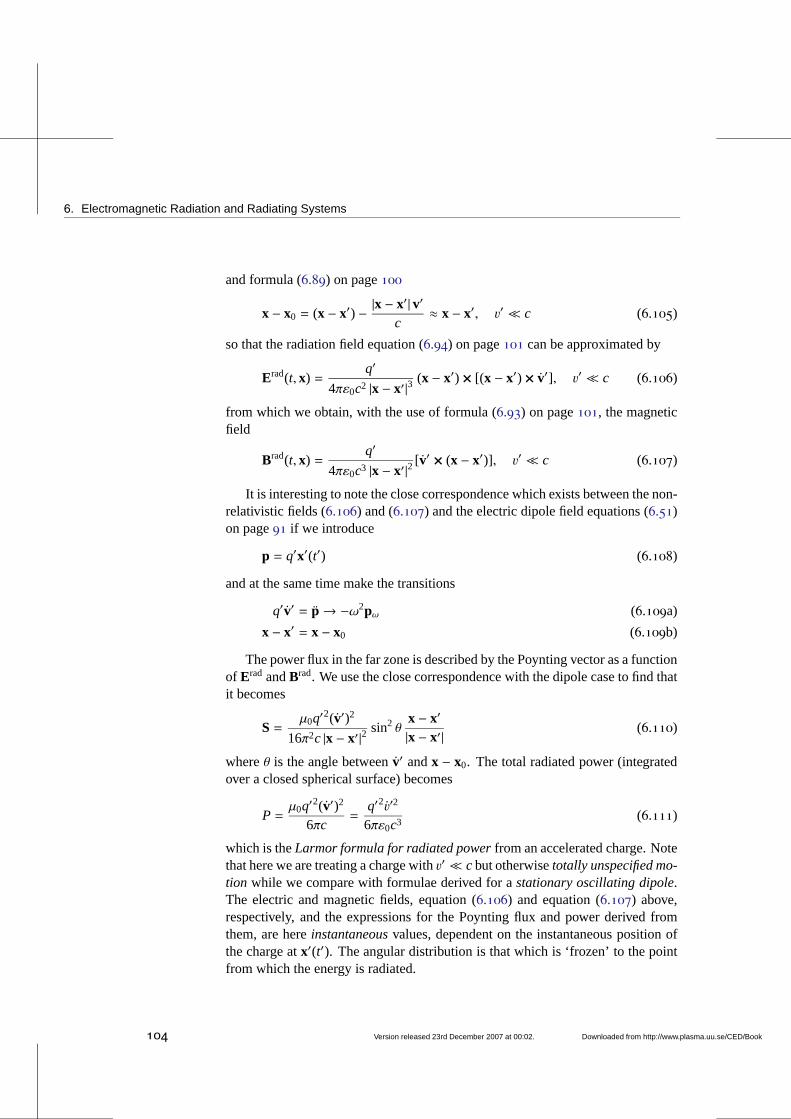
6. Electromagnetic Radiation and Radiating Systems
and formula (6.89) on page100
x − x0 = (x − x′) − |x − x′| v′c
≈ x − x′, v′ ≪ c (6.105)
so that the radiation field equation (6.94) on page101 can be approximated by
Erad(t, x) =q′
4πε0c2 |x − x′|3(x − x′) × [(x − x′) × v′], v′ ≪ c (6.106)
from which we obtain, with the use of formula (6.93) on page101, the magneticfield
Brad(t, x) =q′
4πε0c3 |x − x′|2[v′ × (x − x′)], v′ ≪ c (6.107)
It is interesting to note the close correspondence which exists between the non-relativistic fields (6.106) and (6.107) and the electric dipole field equations (6.51)on page91 if we introduce
p = q′x′(t′) (6.108)
and at the same time make the transitions
q′v′ = p→ −ω2pω (6.109a)
x − x′ = x − x0 (6.109b)
The power flux in the far zone is described by the Poynting vector as a functionof Erad andBrad. We use the close correspondence with the dipole case to find thatit becomes
S=µ0q′
2(v′)2
16π2c |x − x′|2sin2 θ
x − x′
|x − x′| (6.110)
whereθ is the angle betweenv′ andx − x0. The total radiated power (integratedover a closed spherical surface) becomes
P =µ0q′2(v′)2
6πc=
q′2v′2
6πε0c3(6.111)
which is theLarmor formula for radiated powerfrom an accelerated charge. Notethat here we are treating a charge withv′ ≪ c but otherwisetotally unspecified mo-tion while we compare with formulae derived for astationary oscillating dipole.The electric and magnetic fields, equation (6.106) and equation (6.107) above,respectively, and the expressions for the Poynting flux and power derived fromthem, are hereinstantaneousvalues, dependent on the instantaneous position ofthe charge atx′(t′). The angular distribution is that which is ‘frozen’ to the pointfrom which the energy is radiated.
104 Version released 23rd December 2007 at 00:02. Downloaded from http://www.plasma.uu.se/CED/Book
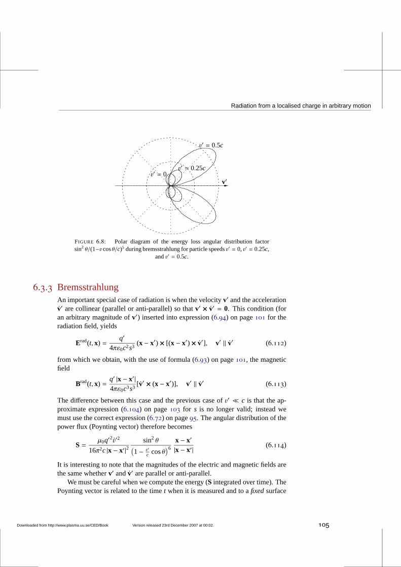
Radiation from a localised charge in arbitrary motion
v′ = 0v′
v′ = 0.5c
v′ = 0.25c
FIGURE 6.8: Polar diagram of the energy loss angular distribution factorsin2 θ/(1−v cosθ/c)5 during bremsstrahlung for particle speedsv′ = 0, v′ = 0.25c,
andv′ = 0.5c.
6.3.3 BremsstrahlungAn important special case of radiation is when the velocityv′ and the accelerationv′ are collinear (parallel or anti-parallel) so thatv′ × v′ = 0. This condition (foran arbitrary magnitude ofv′) inserted into expression (6.94) on page101 for theradiation field, yields
Erad(t, x) =q′
4πε0c2s3(x − x′) × [(x − x′) × v′], v′ ‖ v′ (6.112)
from which we obtain, with the use of formula (6.93) on page101, the magneticfield
Brad(t, x) =q′ |x − x′|4πε0c3s3
[v′ × (x − x′)], v′ ‖ v′ (6.113)
The difference between this case and the previous case ofv′ ≪ c is that the ap-proximate expression (6.104) on page103 for s is no longer valid; instead wemust use the correct expression (6.72) on page95. The angular distribution of thepower flux (Poynting vector) therefore becomes
S=µ0q′2v′2
16π2c |x − x′|2sin2 θ
(1− v′
c cosθ)6
x − x′
|x − x′| (6.114)
It is interesting to note that the magnitudes of the electricand magnetic fields arethe same whetherv′ andv′ are parallel or anti-parallel.
We must be careful when we compute the energy (S integrated over time). ThePoynting vector is related to the timet when it is measured and to afixedsurface
Downloaded from http://www.plasma.uu.se/CED/Book Version released 23rd December 2007 at 00:02. 105
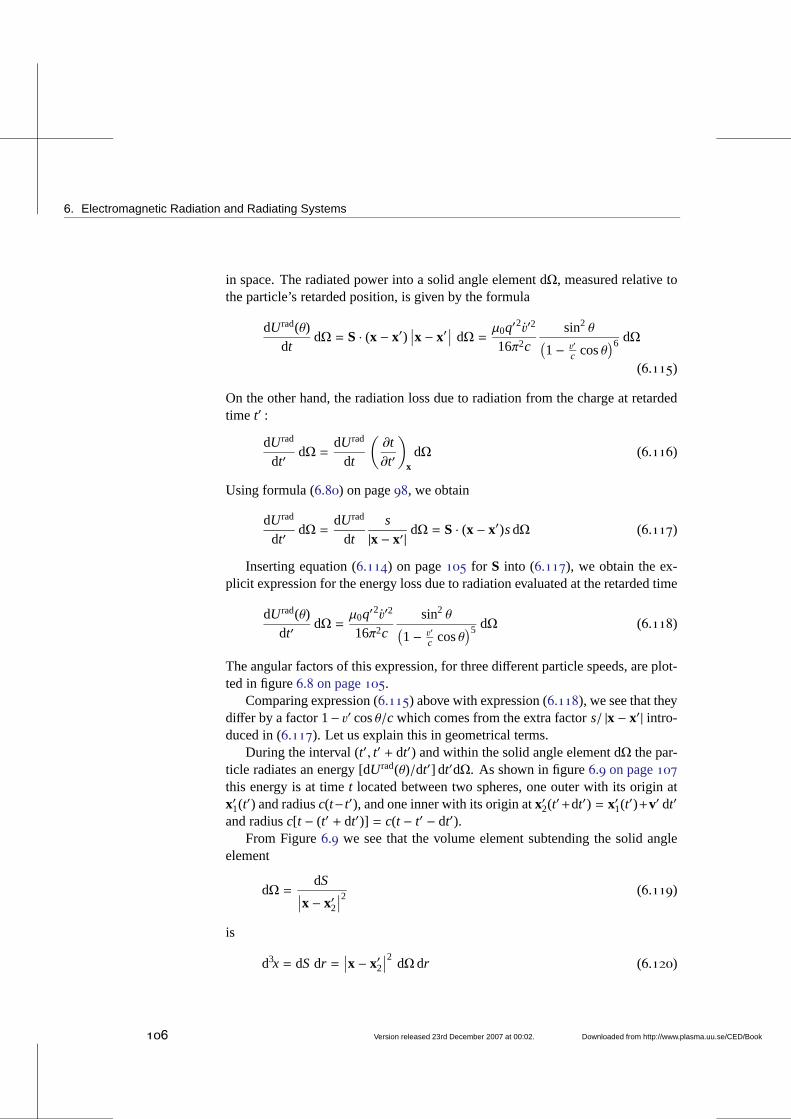
6. Electromagnetic Radiation and Radiating Systems
in space. The radiated power into a solid angle element dΩ, measured relative tothe particle’s retarded position, is given by the formula
dUrad(θ)dt
dΩ = S · (x − x′)∣∣x − x′
∣∣ dΩ =
µ0q′2v′2
16π2csin2 θ
(1− v′
c cosθ)6 dΩ
(6.115)
On the other hand, the radiation loss due to radiation from the charge at retardedtime t′ :
dUrad
dt′dΩ =
dUrad
dt
(∂t∂t′
)
xdΩ (6.116)
Using formula (6.80) on page98, we obtain
dUrad
dt′dΩ =
dUrad
dts
|x − x′| dΩ = S · (x − x′)sdΩ (6.117)
Inserting equation (6.114) on page105 for S into (6.117), we obtain the ex-plicit expression for the energy loss due to radiation evaluated at the retarded time
dUrad(θ)dt′
dΩ =µ0q′2v′2
16π2csin2 θ
(1− v′
c cosθ)5 dΩ (6.118)
The angular factors of this expression, for three different particle speeds, are plot-ted in figure6.8 on page105.
Comparing expression (6.115) above with expression (6.118), we see that theydiffer by a factor 1− v′ cosθ/c which comes from the extra factors/ |x − x′| intro-duced in (6.117). Let us explain this in geometrical terms.
During the interval (t′, t′ + dt′) and within the solid angle element dΩ the par-ticle radiates an energy [dUrad(θ)/dt′] dt′dΩ. As shown in figure6.9 on page107this energy is at timet located between two spheres, one outer with its origin atx′1(t′) and radiusc(t− t′), and one inner with its origin atx′2(t
′+dt′) = x′1(t′)+v′ dt′
and radiusc[t − (t′ + dt′)] = c(t − t′ − dt′).From Figure6.9 we see that the volume element subtending the solid angle
element
dΩ =dS
∣∣x − x′2
∣∣2
(6.119)
is
d3x = dS dr =∣∣x − x′2
∣∣2 dΩ dr (6.120)
106 Version released 23rd December 2007 at 00:02. Downloaded from http://www.plasma.uu.se/CED/Book
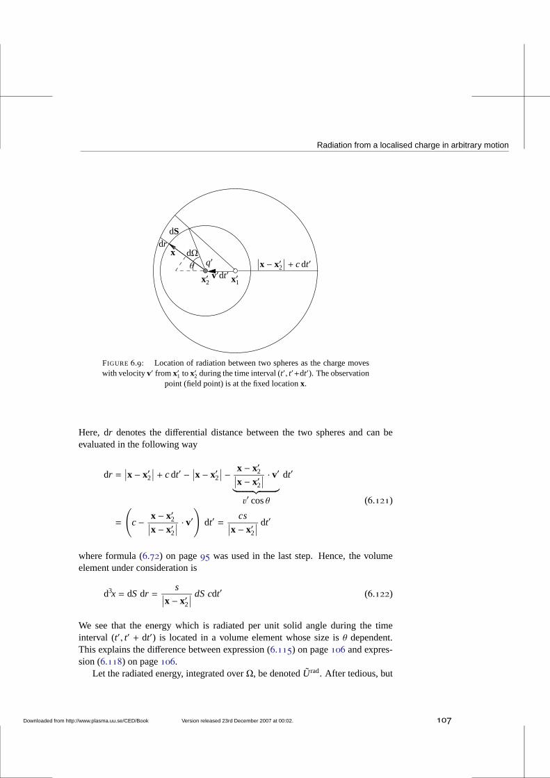
Radiation from a localised charge in arbitrary motion
x′1x′2v′dt′
∣∣x − x′2
∣∣ + cdt′
dSdr
xθ
dΩq′
FIGURE 6.9: Location of radiation between two spheres as the charge moveswith velocityv′ from x′1 to x′2 during the time interval (t′, t′+dt′). The observation
point (field point) is at the fixed locationx.
Here, dr denotes the differential distance between the two spheres and can beevaluated in the following way
dr =∣∣x − x′2
∣∣ + cdt′ −
∣∣x − x′2
∣∣ − x − x′2∣∣x − x′2
∣∣· v′
︸ ︷︷ ︸
v′ cosθ
dt′
=
(
c− x − x′2∣∣x − x′2
∣∣· v′)
dt′ =cs
∣∣x − x′2
∣∣
dt′
(6.121)
where formula (6.72) on page95 was used in the last step. Hence, the volumeelement under consideration is
d3x = dS dr =s
∣∣x − x′2
∣∣
dS cdt′ (6.122)
We see that the energy which is radiated per unit solid angle during the timeinterval (t′, t′ + dt′) is located in a volume element whose size isθ dependent.This explains the difference between expression (6.115) on page106 and expres-sion (6.118) on page106.
Let the radiated energy, integrated overΩ, be denotedUrad. After tedious, but
Downloaded from http://www.plasma.uu.se/CED/Book Version released 23rd December 2007 at 00:02. 107
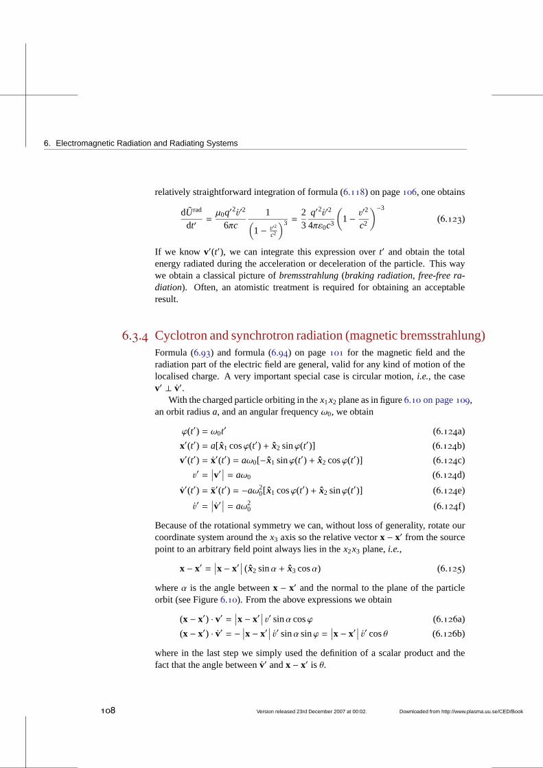
6. Electromagnetic Radiation and Radiating Systems
relatively straightforward integration of formula (6.118) on page106, one obtains
dUrad
dt′=µ0q′2v′2
6πc1
(
1− v′2
c2
)3 =23
q′2v′2
4πε0c3
(
1− v′2
c2
)−3
(6.123)
If we know v′(t′), we can integrate this expression overt′ and obtain the totalenergy radiated during the acceleration or deceleration ofthe particle. This waywe obtain a classical picture ofbremsstrahlung(braking radiation, free-free ra-diation). Often, an atomistic treatment is required for obtaining an acceptableresult.
6.3.4 Cyclotron and synchrotron radiation (magnetic bremsstrahlung)Formula (6.93) and formula (6.94) on page101 for the magnetic field and theradiation part of the electric field are general, valid for any kind of motion of thelocalised charge. A very important special case is circularmotion, i.e., the casev′ ⊥ v′.
With the charged particle orbiting in thex1x2 plane as in figure6.10 on page109,an orbit radiusa, and an angular frequencyω0, we obtain
ϕ(t′) = ω0t′ (6.124a)
x′(t′) = a[ x1 cosϕ(t′) + x2 sinϕ(t′)] (6.124b)
v′(t′) = x′(t′) = aω0[−x1 sinϕ(t′) + x2 cosϕ(t′)] (6.124c)
v′ =∣∣v′∣∣ = aω0 (6.124d)
v′(t′) = x′(t′) = −aω20[ x1 cosϕ(t′) + x2 sinϕ(t′)] (6.124e)
v′ =∣∣v′∣∣ = aω2
0 (6.124f)
Because of the rotational symmetry we can, without loss of generality, rotate ourcoordinate system around thex3 axis so the relative vectorx − x′ from the sourcepoint to an arbitrary field point always lies in thex2x3 plane,i.e.,
x − x′ =∣∣x − x′
∣∣ (x2 sinα + x3 cosα) (6.125)
whereα is the angle betweenx − x′ and the normal to the plane of the particleorbit (see Figure6.10). From the above expressions we obtain
(x − x′) · v′ =∣∣x − x′
∣∣ v′ sinα cosϕ (6.126a)
(x − x′) · v′ = −∣∣x − x′
∣∣ v′ sinα sinϕ =
∣∣x − x′
∣∣ v′ cosθ (6.126b)
where in the last step we simply used the definition of a scalarproduct and thefact that the angle betweenv′ andx − x′ is θ.
108 Version released 23rd December 2007 at 00:02. Downloaded from http://www.plasma.uu.se/CED/Book
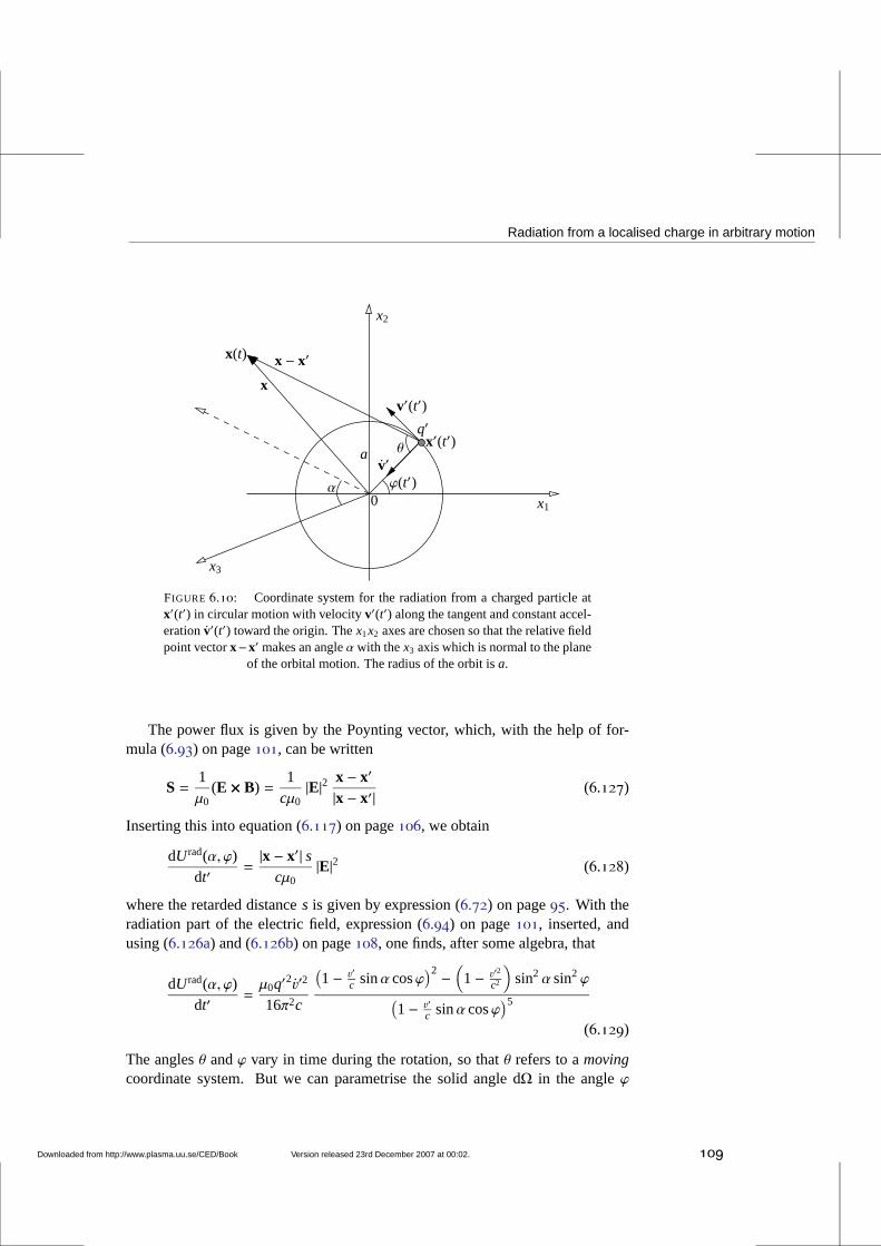
Radiation from a localised charge in arbitrary motion
v′(t′)
x1
x3
x2
ϕ(t′)0
α
av′
x − x′
x
x′(t′)q′
θ
x(t)
FIGURE 6.10: Coordinate system for the radiation from a charged particleatx′(t′) in circular motion with velocityv′(t′) along the tangent and constant accel-erationv′(t′) toward the origin. Thex1x2 axes are chosen so that the relative fieldpoint vectorx−x′ makes an angleα with thex3 axis which is normal to the plane
of the orbital motion. The radius of the orbit isa.
The power flux is given by the Poynting vector, which, with thehelp of for-mula (6.93) on page101, can be written
S=1µ0
(E × B) =1
cµ0|E|2 x − x′
|x − x′| (6.127)
Inserting this into equation (6.117) on page106, we obtain
dUrad(α, ϕ)dt′
=|x − x′| s
cµ0|E|2 (6.128)
where the retarded distances is given by expression (6.72) on page95. With theradiation part of the electric field, expression (6.94) on page101, inserted, andusing (6.126a) and (6.126b) on page108, one finds, after some algebra, that
dUrad(α, ϕ)dt′
=µ0q′2v′2
16π2c
(1− v′
c sinα cosϕ)2 −
(
1− v′2
c2
)
sin2 α sin2 ϕ
(1− v′
c sinα cosϕ)5
(6.129)
The anglesθ andϕ vary in time during the rotation, so thatθ refers to amovingcoordinate system. But we can parametrise the solid angle dΩ in the angleϕ
Downloaded from http://www.plasma.uu.se/CED/Book Version released 23rd December 2007 at 00:02. 109
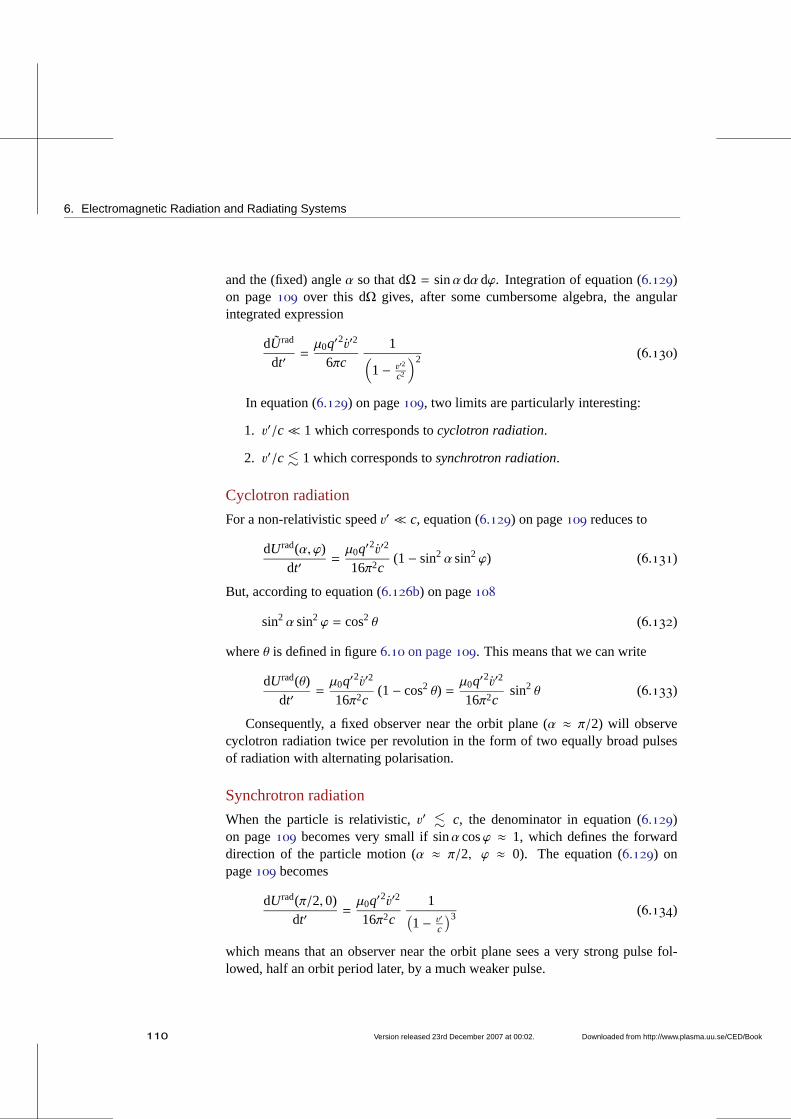
6. Electromagnetic Radiation and Radiating Systems
and the (fixed) angleα so that dΩ = sinαdαdϕ. Integration of equation (6.129)on page109 over this dΩ gives, after some cumbersome algebra, the angularintegrated expression
dUrad
dt′=µ0q′2v′2
6πc1
(
1− v′2
c2
)2 (6.130)
In equation (6.129) on page109, two limits are particularly interesting:
1. v′/c≪ 1 which corresponds tocyclotron radiation.
2. v′/c . 1 which corresponds tosynchrotron radiation.
Cyclotron radiation
For a non-relativistic speedv′ ≪ c, equation (6.129) on page109 reduces to
dUrad(α, ϕ)dt′
=µ0q′
2v′2
16π2c(1− sin2α sin2 ϕ) (6.131)
But, according to equation (6.126b) on page108
sin2 α sin2 ϕ = cos2 θ (6.132)
whereθ is defined in figure6.10 on page109. This means that we can write
dUrad(θ)dt′
=µ0q′2v′2
16π2c(1− cos2 θ) =
µ0q′2v′2
16π2csin2 θ (6.133)
Consequently, a fixed observer near the orbit plane (α ≈ π/2) will observecyclotron radiation twice per revolution in the form of two equally broad pulsesof radiation with alternating polarisation.
Synchrotron radiation
When the particle is relativistic,v′ . c, the denominator in equation (6.129)on page109 becomes very small if sinα cosϕ ≈ 1, which defines the forwarddirection of the particle motion (α ≈ π/2, ϕ ≈ 0). The equation (6.129) onpage109 becomes
dUrad(π/2, 0)dt′
=µ0q′
2v′2
16π2c1
(1− v′
c
)3 (6.134)
which means that an observer near the orbit plane sees a very strong pulse fol-lowed, half an orbit period later, by a much weaker pulse.
110 Version released 23rd December 2007 at 00:02. Downloaded from http://www.plasma.uu.se/CED/Book
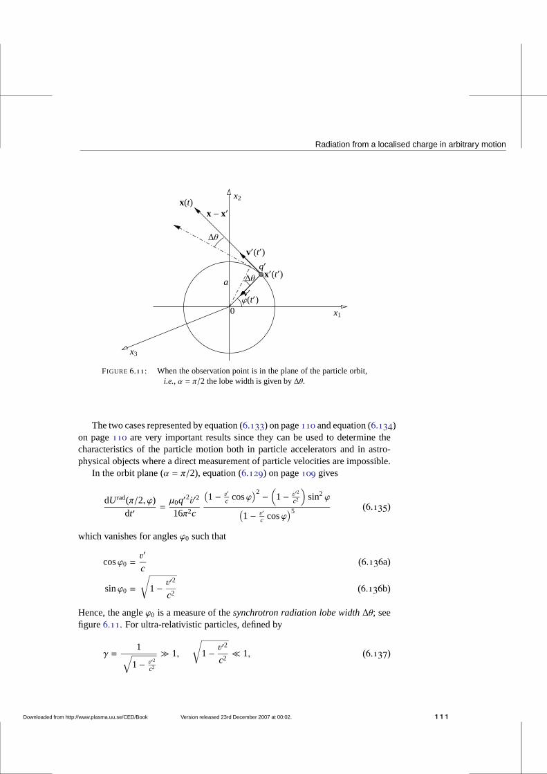
Radiation from a localised charge in arbitrary motion
v′(t′)
x1
x3
x2
ϕ(t′)0
a ∆θ
∆θ
v′
x(t)x − x′
x′(t′)q′
FIGURE 6.11: When the observation point is in the plane of the particle orbit,i.e., α = π/2 the lobe width is given by∆θ.
The two cases represented by equation (6.133) on page110 and equation (6.134)on page110 are very important results since they can be used to determine thecharacteristics of the particle motion both in particle accelerators and in astro-physical objects where a direct measurement of particle velocities are impossible.
In the orbit plane (α = π/2), equation (6.129) on page109 gives
dUrad(π/2, ϕ)dt′
=µ0q′2v′2
16π2c
(1− v′
c cosϕ)2 −
(
1− v′2
c2
)
sin2 ϕ
(1− v′
c cosϕ)5 (6.135)
which vanishes for anglesϕ0 such that
cosϕ0 =v′
c(6.136a)
sinϕ0 =
√
1− v′2
c2(6.136b)
Hence, the angleϕ0 is a measure of thesynchrotron radiation lobe width∆θ; seefigure6.11. For ultra-relativistic particles, defined by
γ =1
√
1− v′2
c2
≫ 1,
√
1− v′2
c2≪ 1, (6.137)
Downloaded from http://www.plasma.uu.se/CED/Book Version released 23rd December 2007 at 00:02. 111
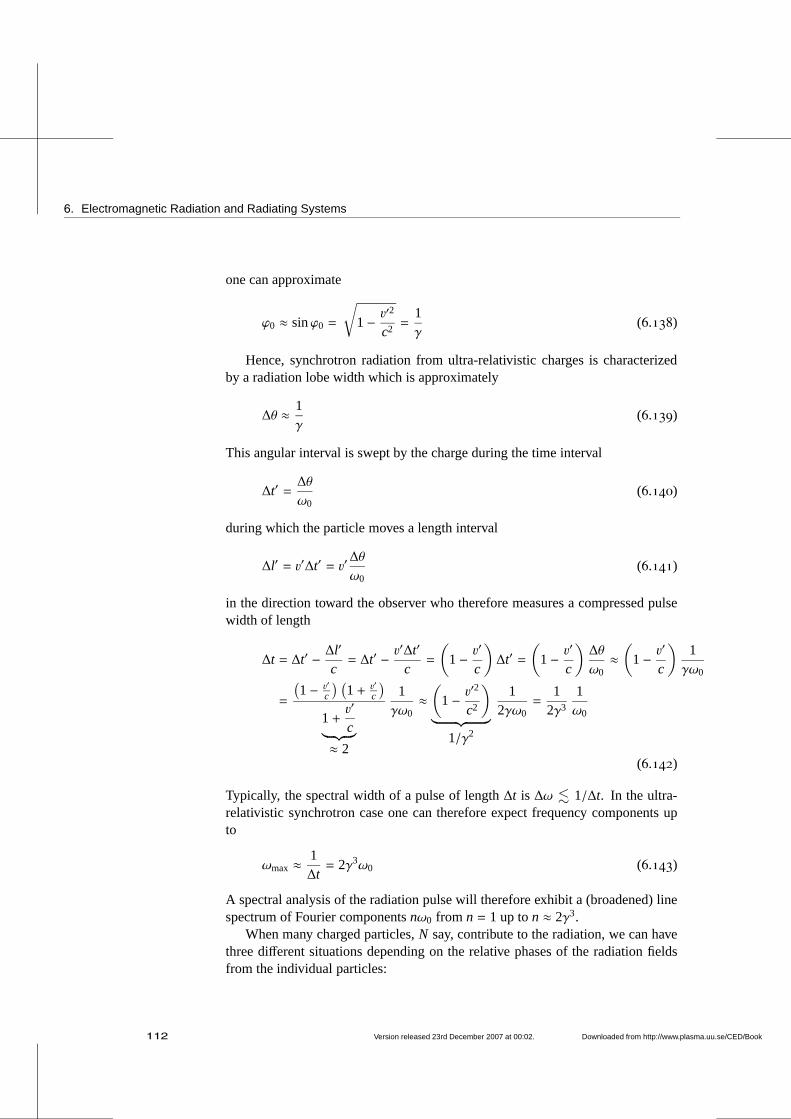
6. Electromagnetic Radiation and Radiating Systems
one can approximate
ϕ0 ≈ sinϕ0 =
√
1− v′2
c2=
1γ
(6.138)
Hence, synchrotron radiation from ultra-relativistic charges is characterizedby a radiation lobe width which is approximately
∆θ ≈ 1γ
(6.139)
This angular interval is swept by the charge during the time interval
∆t′ =∆θ
ω0(6.140)
during which the particle moves a length interval
∆l′ = v′∆t′ = v′∆θ
ω0(6.141)
in the direction toward the observer who therefore measuresa compressed pulsewidth of length
∆t = ∆t′ − ∆l′
c= ∆t′ − v
′∆t′
c=
(
1− v′
c
)
∆t′ =
(
1− v′
c
)∆θ
ω0≈(
1− v′
c
)1γω0
=
(1− v′
c
) (1+ v′
c
)
1+v′
c︸ ︷︷ ︸
≈ 2
1γω0
≈(
1− v′2
c2
)
︸ ︷︷ ︸
1/γ2
12γω0
=1
2γ3
1ω0
(6.142)
Typically, the spectral width of a pulse of length∆t is ∆ω . 1/∆t. In the ultra-relativistic synchrotron case one can therefore expect frequency components upto
ωmax ≈1∆t= 2γ3ω0 (6.143)
A spectral analysis of the radiation pulse will therefore exhibit a (broadened) linespectrum of Fourier componentsnω0 from n = 1 up ton ≈ 2γ3.
When many charged particles,N say, contribute to the radiation, we can havethree different situations depending on the relative phases of the radiation fieldsfrom the individual particles:
112 Version released 23rd December 2007 at 00:02. Downloaded from http://www.plasma.uu.se/CED/Book
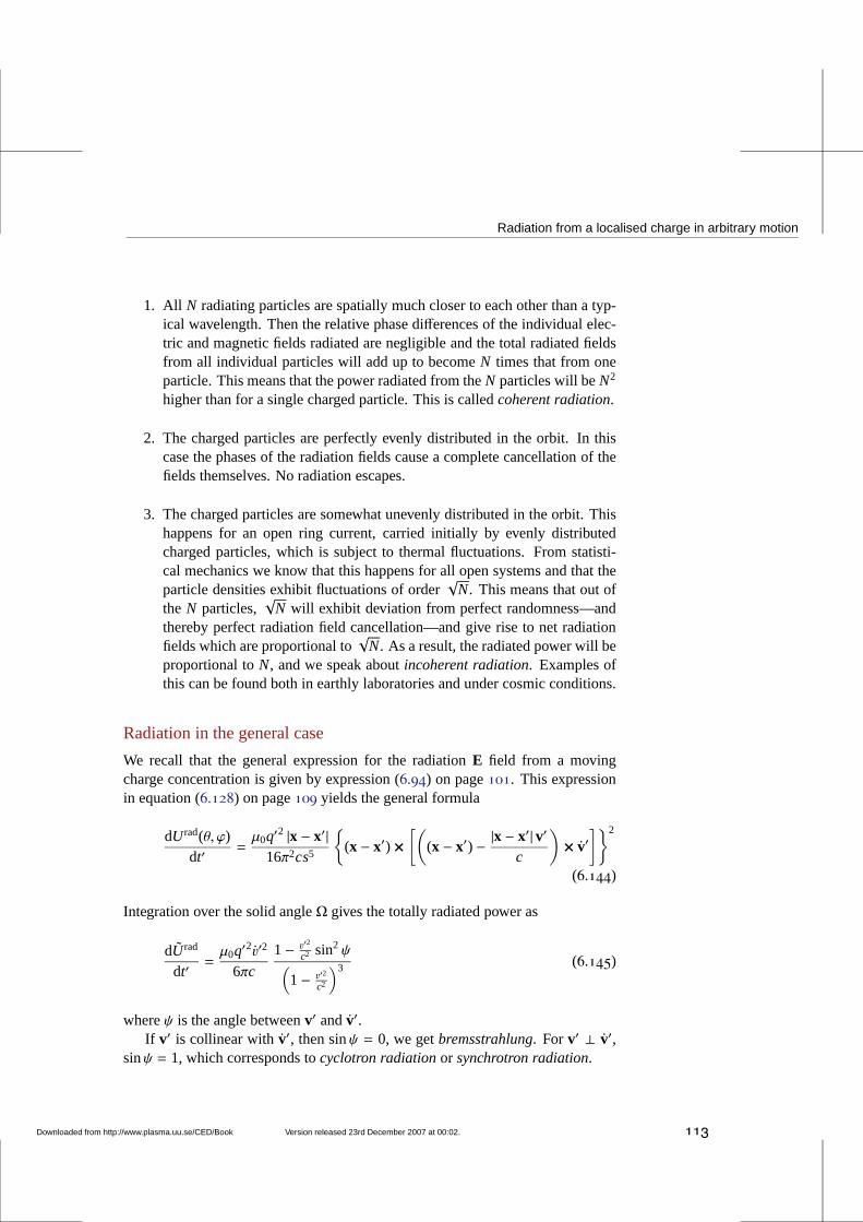
Radiation from a localised charge in arbitrary motion
1. All N radiating particles are spatially much closer to each otherthan a typ-ical wavelength. Then the relative phase differences of the individual elec-tric and magnetic fields radiated are negligible and the total radiated fieldsfrom all individual particles will add up to becomeN times that from oneparticle. This means that the power radiated from theN particles will beN2
higher than for a single charged particle. This is calledcoherent radiation.
2. The charged particles are perfectly evenly distributed in the orbit. In thiscase the phases of the radiation fields cause a complete cancellation of thefields themselves. No radiation escapes.
3. The charged particles are somewhat unevenly distributedin the orbit. Thishappens for an open ring current, carried initially by evenly distributedcharged particles, which is subject to thermal fluctuations. From statisti-cal mechanics we know that this happens for all open systems and that theparticle densities exhibit fluctuations of order
√N. This means that out of
the N particles,√
N will exhibit deviation from perfect randomness—andthereby perfect radiation field cancellation—and give riseto net radiationfields which are proportional to
√N. As a result, the radiated power will be
proportional toN, and we speak aboutincoherent radiation. Examples ofthis can be found both in earthly laboratories and under cosmic conditions.
Radiation in the general case
We recall that the general expression for the radiationE field from a movingcharge concentration is given by expression (6.94) on page101. This expressionin equation (6.128) on page109 yields the general formula
dUrad(θ, ϕ)dt′
=µ0q′2 |x − x′|
16π2cs5
(x − x′) ×[(
(x − x′) − |x − x′| v′c
)
× v′]2
(6.144)
Integration over the solid angleΩ gives the totally radiated power as
dUrad
dt′=µ0q′2v′2
6πc
1− v′2
c2 sin2ψ(
1− v′2
c2
)3 (6.145)
whereψ is the angle betweenv′ andv′.If v′ is collinear withv′, then sinψ = 0, we getbremsstrahlung. For v′ ⊥ v′,
sinψ = 1, which corresponds tocyclotron radiationor synchrotron radiation.
Downloaded from http://www.plasma.uu.se/CED/Book Version released 23rd December 2007 at 00:02. 113
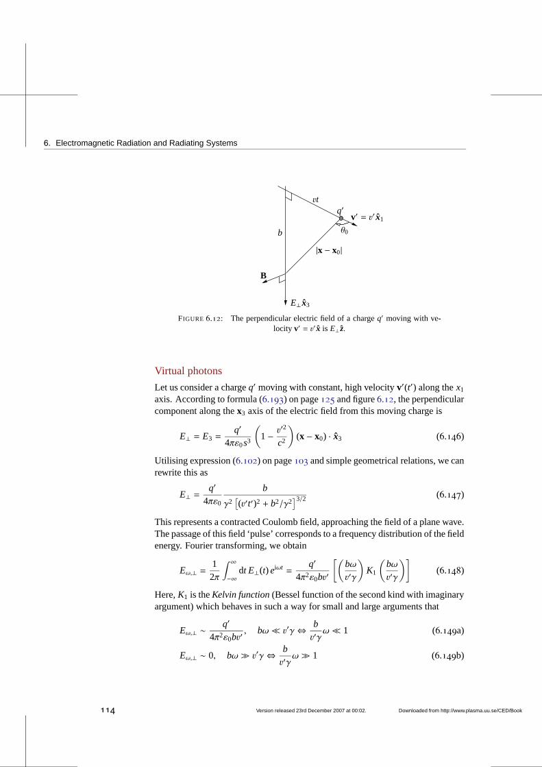
6. Electromagnetic Radiation and Radiating Systems
θ0
vt
b
B
v′ = v′ x1q′
|x − x0|
E⊥ x3
FIGURE 6.12: The perpendicular electric field of a chargeq′ moving with ve-locity v′ = v′ x is E⊥ z.
Virtual photons
Let us consider a chargeq′ moving with constant, high velocityv′(t′) along thex1
axis. According to formula (6.193) on page125 and figure6.12, the perpendicularcomponent along thex3 axis of the electric field from this moving charge is
E⊥ = E3 =q′
4πε0s3
(
1− v′2
c2
)
(x − x0) · x3 (6.146)
Utilising expression (6.102) on page103 and simple geometrical relations, we canrewrite this as
E⊥ =q′
4πε0
b
γ2[(v′t′)2 + b2/γ2
]3/2 (6.147)
This represents a contracted Coulomb field, approaching thefield of a plane wave.The passage of this field ‘pulse’ corresponds to a frequency distribution of the fieldenergy. Fourier transforming, we obtain
Eω,⊥ =12π
∫ ∞
−∞dt E⊥(t) eiωt =
q′
4π2ε0bv′
[(bωv′γ
)
K1
(bωv′γ
)]
(6.148)
Here,K1 is theKelvin function(Bessel function of the second kind with imaginaryargument) which behaves in such a way for small and large arguments that
Eω,⊥ ∼q′
4π2ε0bv′, bω ≪ v′γ ⇔ b
v′γω ≪ 1 (6.149a)
Eω,⊥ ∼ 0, bω ≫ v′γ ⇔ bv′γ
ω ≫ 1 (6.149b)
114 Version released 23rd December 2007 at 00:02. Downloaded from http://www.plasma.uu.se/CED/Book
Radiation from a localised charge in arbitrary motion
showing that the ‘pulse’ length is of the orderb/(v′γ).Due to the equipartitioning of the field energy into the electric and magnetic
fields, the total field energy can be written
U = ε0
∫
Vd3x E2
⊥ = ε0
∫ bmax
bmin
db2πb∫ ∞
−∞dt v′E2
⊥ (6.150)
where the volume integration is over the plane perpendicular to v′. With the useof Parseval’s identityfor Fourier transforms, formula (5.34) on page75, we canrewrite this as
U =∫ ∞
0dω Uω = 4πε0v
′∫ bmax
bmin
db2πb∫ ∞
0dωE2
ω,⊥
≈ q′2
2π2ε0v′
∫ ∞
−∞dω∫ v′γ/ω
bmin
dbb
(6.151)
from which we conclude that
Uω ≈q′2
2π2ε0v′ln
(v′γ
bminω
)
(6.152)
where an explicit value ofbmin can be calculated in quantum theory only.As in the case of bremsstrahlung, it is intriguing to quantise the energy into
photons [cf. equation (6.223) on page129]. Then we find that
Nω dω ≈ 2απ
ln
(cγ
bminω
)dωω
(6.153)
whereα = e2/(4πε0~c) ≈ 1/137 is thefine structure constant.Let us consider the interaction of two (classical) electrons, 1 and 2. The result
of this interaction is that they change their linear momentafrom p1 to p′1 andp2 top′2, respectively. Heisenberg’s uncertainty principle givesbmin ∼ ~/
∣∣p1 − p′1
∣∣ so
that the number of photons exchanged in the process is of the order
Nω dω ≈ 2απ
ln( cγ
~ω
∣∣p1 − p′1
∣∣
) dωω
(6.154)
Since this change in momentum corresponds to a change in energy ~ω = E1 − E′1andE1 = m0γc2, we see that
Nω dω ≈ 2απ
ln
(
E1
m0c2
∣∣cp1 − cp′1
∣∣
E1 − E′1
)
dωω
(6.155)
a formula which gives a reasonable semi-classical account of a photon-inducedelectron-electron interaction process. In quantum theory, including only the low-est order contributions, this process is known asMøller scattering. A diagram-matic representation of (a semi-classical approximation of) this process is givenin figure6.13 on page116.
Downloaded from http://www.plasma.uu.se/CED/Book Version released 23rd December 2007 at 00:02. 115
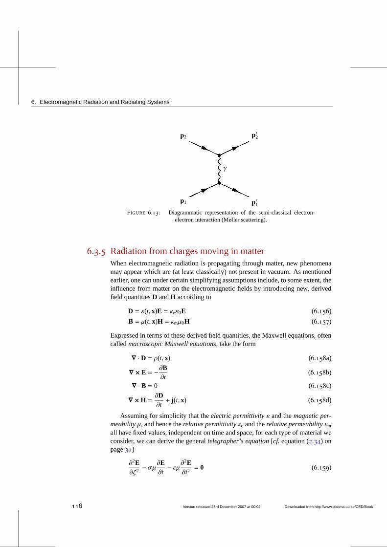
6. Electromagnetic Radiation and Radiating Systems
γ
p1
p2
p′1
p′2
FIGURE 6.13: Diagrammatic representation of the semi-classical electron-electron interaction (Møller scattering).
6.3.5 Radiation from charges moving in matterWhen electromagnetic radiation is propagating through matter, new phenomenamay appear which are (at least classically) not present in vacuum. As mentionedearlier, one can under certain simplifying assumptions include, to some extent, theinfluence from matter on the electromagnetic fields by introducing new, derivedfield quantitiesD andH according to
D = ε(t, x)E = κeε0E (6.156)
B = µ(t, x)H = κmµ0H (6.157)
Expressed in terms of these derived field quantities, the Maxwell equations, oftencalledmacroscopic Maxwell equations, take the form
∇ · D = ρ(t, x) (6.158a)
∇ × E = −∂B∂t
(6.158b)
∇ · B = 0 (6.158c)
∇ × H =∂D∂t+ j (t, x) (6.158d)
Assuming for simplicity that theelectric permittivityε and themagnetic per-meabilityµ, and hence therelative permittivityκe and therelative permeabilityκm
all have fixed values, independent on time and space, for eachtype of material weconsider, we can derive the generaltelegrapher’s equation[cf. equation (2.34) onpage31]
∂2E∂ζ2− σµ∂E
∂t− εµ∂
2E∂t2= 0 (6.159)
116 Version released 23rd December 2007 at 00:02. Downloaded from http://www.plasma.uu.se/CED/Book
Radiation from a localised charge in arbitrary motion
describing (1D) wave propagation in a material medium.In chapter2 we concluded that the existence of a finite conductivity, manifest-
ing itself in acollisional interactionbetween the charge carriers, causes the wavesto decay exponentially with time and space. Let us thereforeassume that in ourmediumσ = 0 so that the wave equation simplifies to
∂2E∂ζ2− εµ∂
2E∂t2= 0 (6.160)
If we introduce thephase velocityin the medium as
vϕ =1√εµ=
1√κeε0κmµ0
=c√κeκm
(6.161)
where, according to equation (1.11) on page6, c = 1/√ε0µ0 is the speed of
light, i.e., the phase speed of electromagnetic waves in vacuum, then the generalsolution to each component of equation (6.160)
Ei = f (ζ − vϕt) + g(ζ + vϕt), i = 1, 2, 3 (6.162)
The ratio of the phase speed in vacuum and in the medium
cvϕ=√κeκm = c
√εµ
def≡ n (6.163)
is called therefractive indexof the medium. In generaln is a function of bothtime and space as are the quantitiesε, µ, κe, andκm themselves. If, in addition,the medium isanisotropicor birefringent, all these quantities are rank-two tensorfields. Under our simplifying assumptions, in each medium weconsidern =Constfor each frequency component of the fields.
Associated with the phase speed of a medium for a wave of a given frequencyω we have awave vector, defined as
kdef≡ kk = kvϕ =
ω
vϕ
vϕvϕ
(6.164)
As in the vacuum case discussed in chapter2, assuming thatE is time-harmonic,i.e., can be represented by a Fourier component proportional to exp−iωt, thesolution of equation (6.160) can be written
E = E0ei(k·x−ωt) (6.165)
where nowk is the wave vectorin the mediumgiven by equation (6.164) above.With these definitions, the vacuum formula for the associated magnetic field,equation (2.41) on page31,
B =√εµ k × E =
1vϕ
k × E =1ω
k × E (6.166)
Downloaded from http://www.plasma.uu.se/CED/Book Version released 23rd December 2007 at 00:02. 117
6. Electromagnetic Radiation and Radiating Systems
is valid also in a material medium (assuming, as mentioned, that n has a fixedconstant scalar value). A consequence of aκe , 1 is that the electric field will, ingeneral, have a longitudinal component.
It is important to notice that depending on the electric and magnetic propertiesof a medium, and, hence, on the value of the refractive indexn, the phase speedin the medium can be smaller or larger than the speed of light:
vϕ =cn=ω
k(6.167)
where, in the last step, we used equation (6.164) on page117.If the medium has a refractive index which, as is usually the case, dependent
on frequencyω, we say that the medium isdispersive. Because in this case alsok(ω) andω(k), so that thegroup velocity
vg =∂ω
∂k(6.168)
has a unique value for each frequency component, and is different fromvϕ. Exceptin regions ofanomalous dispersion, vg is always smaller thanc. In a gas of freecharges, such as aplasma, the refractive index is given by the expression
n2(ω) = 1−ω2
p
ω2(6.169)
where
ω2p =∑
σ
Nσq2σ
ε0mσ
(6.170)
is the square of theplasma frequencyωp. Heremσ andNσ denote the mass andnumber density, respectively, of charged particle speciesσ. In an inhomogeneousplasma,Nσ = Nσ(x) so that the refractive index and also the phase and groupvelocities are space dependent. As can be easily seen, for each given frequency,the phase and group velocities in a plasma are different from each other. If thefrequencyω is such that it coincides withωp at some point in the medium, then atthat pointvϕ → ∞ while vg→ 0 and the wave Fourier component atω is reflectedthere.
Vavilov-Cerenkov radiation
As we saw in subsection6.1, a charge in uniform, rectilinear motionin vacuumdoes not give rise to any radiation; see in particular equation (6.191a) on page124.Let us now consider a charge in uniform, rectilinear motionin a mediumwith elec-tric properties which are different from those of a (classical) vacuum. Specifically,
118 Version released 23rd December 2007 at 00:02. Downloaded from http://www.plasma.uu.se/CED/Book
Radiation from a localised charge in arbitrary motion
consider a medium where
ε = Const> ε0 (6.171a)
µ = µ0 (6.171b)
This implies that in this medium the phase speed is
vϕ =cn=
1√εµ0
< c (6.172)
Hence, in this particular medium, the speed of propagation of (the phase planes of)electromagnetic waves is less than the speed of light in vacuum, which we knowis an absolute limit for the motion of anything, including particles. A mediumof this kind has the interesting property that particles, entering into the mediumat high speeds|v′|, which, of course, are below the phase speedin vacuum, canexperience that the particle speeds arehigher than the phase speedin the medium.This is the basis for theVavilov-Cerenkov radiation, more commonly known asCerenkov radiation, that we shall now study.
If we recall the general derivation, in the vacuum case, of the retarded (and ad-vanced) potentials in chapter3 and the Liénard-Wiechert potentials, equations (6.71)on page95, we realise that we obtain the latter in the medium by a simplefor-mal replacementc → c/n in the expression (6.72) on page95 for s. Hence, theLiénard-Wiechert potentials in a medium characterized by arefractive indexn,are
φ(t, x) =1
4πε0
q′∣∣|x − x′| − n(x−x′)·v′
c
∣∣=
14πε0
q′
s(6.173a)
A(t, x) =1
4πε0c2
q′v′∣∣|x − x′| − n(x−x′)·v′
c
∣∣=
14πε0c2
q′v′
s(6.173b)
where now
s=
∣∣∣∣
∣∣x − x′
∣∣ − n
(x − x′) · v′c
∣∣∣∣
(6.174)
The need for the absolute value of the expression fors is obvious in the casewhenv′/c ≥ 1/n because then the second term can be larger than the first term;if v′/c ≪ 1/n we recover the well-known vacuum case but with modified phasespeed. We also note that the retarded and advanced times in the medium are [cf.equation (3.32) on page46]
t′ret = t′ret(t,∣∣x − x′
∣∣) = t − k |x − x′|
ω= t − |x − x′| n
c(6.175a)
t′adv = t′adv(t,∣∣x − x′
∣∣) = t +
k |x − x′|ω
= t +|x − x′| n
c(6.175b)
Downloaded from http://www.plasma.uu.se/CED/Book Version released 23rd December 2007 at 00:02. 119
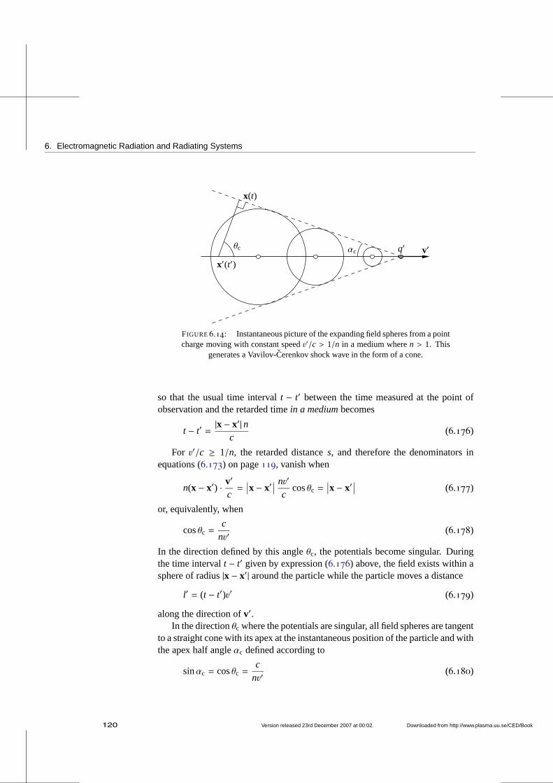
6. Electromagnetic Radiation and Radiating Systems
θc αc v′q′
x′(t′)
x(t)
FIGURE6.14: Instantaneous picture of the expanding field spheres from a pointcharge moving with constant speedv′/c > 1/n in a medium wheren > 1. This
generates a Vavilov-Cerenkov shock wave in the form of a cone.
so that the usual time intervalt − t′ between the time measured at the point ofobservation and the retarded timein a mediumbecomes
t − t′ =|x − x′| n
c(6.176)
For v′/c ≥ 1/n, the retarded distances, and therefore the denominators inequations (6.173) on page119, vanish when
n(x − x′) · v′
c=∣∣x − x′
∣∣
nv′
ccosθc =
∣∣x − x′
∣∣ (6.177)
or, equivalently, when
cosθc =c
nv′(6.178)
In the direction defined by this angleθc, the potentials become singular. Duringthe time intervalt − t′ given by expression (6.176) above, the field exists within asphere of radius|x − x′| around the particle while the particle moves a distance
l′ = (t − t′)v′ (6.179)
along the direction ofv′.In the directionθc where the potentials are singular, all field spheres are tangent
to a straight cone with its apex at the instantaneous position of the particle and withthe apex half angleαc defined according to
sinαc = cosθc =c
nv′(6.180)
120 Version released 23rd December 2007 at 00:02. Downloaded from http://www.plasma.uu.se/CED/Book
Radiation from a localised charge in arbitrary motion
This cone of potential singularities and field sphere circumferences propagateswith speedc/n in the form of ashock front, calledVavilov-Cerenkov radiation.1
TheVavilov-Cerenkov coneis similar in nature to theMach conein acoustics.In order to make some quantitative estimates of this radiation, we note that we
can describe the motion of each charged particleq′ as a current density:
j = q′v′ δ(x′ − v′t′) = q′v′ δ(x′ − v′t′)δ(y′)δ(z′)x1 (6.181)
which has the trivial Fourier transform
jω =q′
2πeiωx′/v′ δ(y′)δ(z′)x1 (6.182)
This Fourier component can be used in the formulae derived for a linear currentin subsection6.1.1 if only we make the replacements
ε0→ ε = n2ε0 (6.183a)
k→ nωc
(6.183b)
In this manner, usingjω from equation (6.182), the resulting Fourier transformsof the Vavilov-Cerenkov magnetic and electric radiation fields can be calculatedfrom the expressions (5.10) on page68) and (5.21) on page70, respectively.
The total energy content is then obtained from equation (5.34) on page75(integrated over a closed sphere at large distances). For a Fourier component oneobtains [cf. equation (5.37) on page76]
Uradω dΩ ≈ 1
4πε0nc
∣∣∣∣
∫
V′d3x′ (jω × k)e−ik·x′
∣∣∣∣
2
dΩ
=q′2nω2
16π3ε0c3
∣∣∣∣
∫ ∞
−∞exp
[
ix′(ω
v′− kcosθ
)]
dx′∣∣∣∣
2
sin2 θ dΩ
(6.184)
1The first systematic exploration of this radiation was made by P. A. Cerenkov in 1934, who was thena post-graduate student in S. I. Vavilov’s research group atthe Lebedev Institute in Moscow. Vavilov wrotea manuscript with the experimental findings, putCerenkov as the author, and submitted it toNature. Inthe manuscript, Vavilov explained the results in terms of radioactive particles creating Compton electronswhich gave rise to the radiation (which was the correct interpretation), but the paper was rejected. Thepaper was then sent toPhysical Reviewand was, after some controversy with the American editors whoclaimed the results to be wrong, eventually published in 1937. In the same year, I. E. Tamm and I. M. Frankpublished the theory for the effect (‘the singing electron’). In fact, predictions of a similar effect had beenmade as early as 1888 by Heaviside, and by Sommerfeld in his 1904 paper ‘Radiating body moving withvelocity of light’. On May 8, 1937, Sommerfeld sent a letter to Tamm via Austria, saying that he wassurprised that his old 1904 ideas were now becoming interesting. Tamm, Frank andCerenkov receivedthe Nobel Prize in 1958 ‘for the discovery and the interpretation of theCerenkov effect’ [V. L. Ginzburg,private communication].The first observation of this type of radiation was reported by Marie Curie in 1910, but she never pursuedthe exploration of it [8].
Downloaded from http://www.plasma.uu.se/CED/Book Version released 23rd December 2007 at 00:02. 121
6. Electromagnetic Radiation and Radiating Systems
whereθ is the angle between the direction of motion,x′1, and the direction to theobserver,k. The integral in (6.184) is singular of a ‘Dirac delta type’. If we limitthe spatial extent of the motion of the particle to the closedinterval [−X,X] on thex′ axis we can evaluate the integral to obtain
Uradω dΩ =
q′2nω2 sin2 θ
4π3ε0c3
sin2[(
1− nv′
c cosθ)
Xωv′
]
[(1− nv′
c cosθ)ωv′
]2 dΩ (6.185)
which has a maximum in the directionθc as expected. The magnitude of thismaximum grows and its width narrows asX → ∞. The integration of (6.185)overΩ therefore picks up the main contributions fromθ ≈ θc. Consequently, wecan set sin2 θ ≈ sin2 θc and the result of the integration is
Uradω = 2π
∫ π
0Uradω (θ) sinθ dθ = ⌈cosθ = −ξ⌋ = 2π
∫ 1
−1Uradω (ξ) dξ
≈ q′2nω2 sin2 θc
2π2ε0c3
∫ 1
−1
sin2[(
1+ nv′ξc
)Xωv′
]
[(1+ nv′ξ
c
)ωv′
]2 dξ
(6.186)
The integrand in (6.186) is strongly peaked nearξ = −c/(nv′), or, equivalently,near cosθc = c/(nv′). This means that the integrand function is practically zerooutside the integration intervalξ ∈ [−1, 1]. Consequently, one may extend theξ integration interval to (−∞,∞) without introducing too much an error. Via yetanother variable substitution we can therefore approximate
sin2 θc
∫ 1
−1
sin2[(
1+ nv′ξc
)Xωv′
]
[(1+ nv′ξ
c
)ωv′
]2 dξ ≈(
1− c2
n2v′2
)cXωn
∫ ∞
−∞
sin2 xx2
dx
=cXπωn
(
1− c2
n2v′2
)
(6.187)
leading to the final approximate result for the total energy loss in the frequencyinterval (ω,ω + dω)
Uradω dω =
q′2X2πε0c2
(
1− c2
n2v′2
)
ωdω (6.188)
As mentioned earlier, the refractive index is usually frequency dependent. Re-alising this, we find that the radiation energy per frequencyunit andper unit lengthis
Uradω dω2X
=q′2ω
4πε0c2
(
1− c2
n2(ω)v′2
)
dω (6.189)
122 Version released 23rd December 2007 at 00:02. Downloaded from http://www.plasma.uu.se/CED/Book
Bibliography
This result was derived under the assumption thatv′/c > 1/n(ω), i.e., under thecondition that the expression inside the parentheses in theright hand side is pos-itive. For all media it is true thatn(ω) → 1 whenω → ∞, so there exist alwaysa highest frequency for which we can obtain Vavilov-Cerenkov radiation from afast charge in a medium. Our derivation above for a fixed valueof n is valid foreach individual Fourier component.
6.4 Bibliography[1] H. ALFVÉN AND N. HERLOFSON, Cosmic radiation and radio stars,Physical Review, 78
(1950), p. 616.
[2] R. BECKER, Electromagnetic Fields and Interactions, Dover Publications, Inc.,New York, NY, 1982, ISBN 0-486-64290-9.
[3] M. BORN AND E. WOLF, Principles of Optics. Electromagnetic Theory of Propaga-tion, Interference and Diffraction of Light, sixth ed., Pergamon Press, Oxford,. . . , 1980,ISBN 0-08-026481-6.
[4] V. L. GINZBURG, Applications of Electrodynamics in Theoretical Physics and Astro-physics, Revised third ed., Gordon and Breach Science Publishers, New York, London,Paris, Montreux, Tokyo and Melbourne, 1989, ISBN 2-88124-719-9.
[5] J. D. JACKSON, Classical Electrodynamics, third ed., John Wiley & Sons, Inc.,New York, NY . . . , 1999, ISBN 0-471-30932-X.
[6] J. B. MARION AND M. A. HEALD, Classical Electromagnetic Radiation, second ed.,Academic Press, Inc. (London) Ltd., Orlando, . . . , 1980, ISBN 0-12-472257-1.
[7] W. K. H. PANOFSKY AND M. PHILLIPS, Classical Electricity and Magnetism, second ed.,Addison-Wesley Publishing Company, Inc., Reading, MA . . . ,1962, ISBN 0-201-05702-6.
[8] J. SCHWINGER, L. L. DERAAD , JR., K. A. M ILTON , AND W. TSAI, Classical Electrody-namics, Perseus Books, Reading, MA, 1998, ISBN 0-7382-0056-5.18, 121
[9] J. A. STRATTON, Electromagnetic Theory, McGraw-Hill Book Company, Inc., NewYork, NY and London, 1953, ISBN 07-062150-0.
[10] J. VANDERLINDE, Classical Electromagnetic Theory, John Wiley & Sons, Inc., NewYork, Chichester, Brisbane, Toronto, and Singapore, 1993,ISBN 0-471-57269-1.
Downloaded from http://www.plasma.uu.se/CED/Book Version released 23rd December 2007 at 00:02. 123
6. Electromagnetic Radiation and Radiating Systems
6.5 Examples
⊲THE FIELDS FROM A UNIFORMLY MOVING CHARGEEXAMPLE 6.1
In the special case of uniform motion, the localised charge moves in a field-free, isolatedspace and we know that it will not be affected by any external forces. It will therefore move uni-formly in a straight line with the constant velocityv′. This gives us the possibility to extrapolateits position at the observation time,x′(t), from its position at the retarded time,x′(t′). Since theparticle is not accelerated,v′ ≡ 0, the virtual simultaneous coordinatex0 will be identical tothe actualsimultaneous coordinateof the particle at timet, i.e., x0(t) = x′(t). As depicted infigure6.7 on page96, the angle betweenx− x0 andv′ is θ0 while then angle betweenx− x′ andv′ is θ′.
We note that in the case of uniform velocityv′, time and space derivatives are closely relatedin the following way when they operate on functions ofx(t) [cf. equation (1.33) on page13]:
∂
∂t→ −v′ · ∇ (6.190)
Hence, theE andB fields can be obtained from formulae (6.73) on page96, with the potentialsgiven by equations (6.71) on page95 as follows:
E = −∇φ − ∂A∂t= −∇φ − 1
c2
∂v′φ∂t= −∇φ − v′
c2
∂φ
∂t
= −∇φ + v′
c
(v′
c· ∇φ
)
= −(
1− v′v′
c2·)
∇φ
=
(v′v′
c2− 1
)
· ∇φ
(6.191a)
B = ∇ × A = ∇ ×(
v′
c2φ
)
= ∇φ ×v′
c2= − v′
c2× ∇φ
=v′
c2×
[(v′
c· ∇φ
)v′
c− ∇φ
]
=v′
c2×
(v′v′
c2− 1
)
· ∇φ
=v′
c2× E
(6.191b)
Here1 = xi xi is the unit dyad and we used the fact thatv′ × v′ ≡ 0. What remains is just toexpress∇φ in quantities evaluated att andx.
From equation (6.71a) on page95 and equation (6.103) on page103 we find that
∇φ =q′
4πε0∇
(1s
)
= − q′
8πε0s3∇s2
= − q′
4πε0s3
[
(x − x0) +v′
c×
(v′
c× (x − x0)
)] (6.192)
When this expression for∇φ is inserted into equation (6.191a) above, the following result
124 Version released 23rd December 2007 at 00:02. Downloaded from http://www.plasma.uu.se/CED/Book
Examples
E(t, x) =
(v′v′
c2− 1
)
· ∇φ = − q′
8πε0s3
(v′v′
c2− 1
)
· ∇s2
=q′
4πε0s3
(x − x0) +v′
c×
(v′
c× (x − x0)
)
− v′
c
(v′
c· (x − x0)
)
− v′v′
c2·[
v′
c×
(v′
c× (x − x0)
)]
=q′
4πε0s3
[
(x − x0) +v′
c
(v′
c· (x − x0)
)
− (x − x0)v′2
c2
− v′
c
(v′
c· (x − x0)
)]
=q′
4πε0s3(x − x0)
(
1− v′2
c2
)
(6.193)
follows. Of course, the same result also follows from equation (6.90) on page100 with v′ ≡ 0inserted.
From equation (6.193) above we conclude thatE is directed along the vector from thesimultaneous coordinatex0(t) to the field (observation) coordinatex(t). In a similar way, themagnetic field can be calculated and one finds that
B(t, x) =µ0q′
4πs3
(
1− v′2
c2
)
v′ × (x − x0) =1c2
v′ × E (6.194)
From these explicit formulae for theE andB fields and formula (6.102b) on page103 for s, wecan discern the following cases:
1. v′ → 0⇒ E goes over into the Coulomb fieldECoulomb
2. v′ → 0⇒ B goes over into the Biot-Savart field
3. v′ → c⇒ E becomes dependent onθ0
4. v′ → c, sinθ0 ≈ 0⇒ E→ (1− v′2/c2)ECoulomb
5. v′ → c, sinθ0 ≈ 1⇒ E→ (1− v′2/c2)−1/2ECoulomb
⊳ END OF EXAMPLE 6.1
⊲THE CONVECTION POTENTIAL AND THE CONVECTION FORCE EXAMPLE 6.2
Let us consider in more detail the treatment of the radiationfrom a uniformly moving rigidcharge distribution.
If we return to the original definition of the potentials and the inhomogeneous wave equa-tion, formula (3.17) on page43, for a generic potential componentΨ(t, x) and a generic sourcecomponentf (t, x),
2Ψ(t, x) =
(1c2
∂2
∂t2− ∇2
)
Ψ(t, x) = f (t, x) (6.195)
Downloaded from http://www.plasma.uu.se/CED/Book Version released 23rd December 2007 at 00:02. 125
6. Electromagnetic Radiation and Radiating Systems
we find that under the assumption thatv′ = v′ x1, this equation can be written(
1− v′2
c2
)∂2Ψ
∂x21
+∂2Ψ
∂x22
+∂2Ψ
∂x23
= − f (x) (6.196)
i.e., in a time-independent form. Transforming
ξ1 =x1√
1− v′2/c2(6.197a)
ξ2 = x2 (6.197b)
ξ3 = x3 (6.197c)
and introducing the vectorial nabla operator inξ space,∇ξ ≡def (∂/∂ξ1, ∂/∂ξ2, ∂/∂ξ3), the time-independent equation (??) reduces to an ordinaryPoisson equation
∇2ξΨ(ξ) = − f (
√
1− v′2/c2 ξ1, ξ2, ξ3) ≡ − f (ξ) (6.198)
in this space. This equation has the well-known Coulomb potential solution
Ψ(ξ) =14π
∫
V
f (ξ′)|ξ − ξ′| d
3ξ′ (6.199)
After inverse transformation back to the original coordinates, this becomes
Ψ(x) =14π
∫
V
f (x′)s
d3x′ (6.200)
where, in the denominator,
s=
[
(x1 − x′1)2 +
(
1− v′2
c2
)
[(x2 − x′2)2 + (x3 − x′3)2]
] 12
(6.201)
Applying this to the explicit scalar and vector potential components, realising that for a rigidcharge distributionρ moving with velocityv′ the current is given byj = ρv′, we obtain
φ(t, x) =1
4πε0
∫
V
ρ(x′)s
d3x′ (6.202a)
A(t, x) =1
4πε0c2
∫
V
v′ρ(x′)s
d3x′ =v′
c2φ(t, x) (6.202b)
For a localised charge where∫
ρ d3x′ = q′, these expressions reduce to
φ(t, x) =q′
4πε0s(6.203a)
A(t, x) =q′v′
4πε0c2s(6.203b)
which we recognise as theLiénard-Wiechert potentials; cf. equations (6.71) on page95. Wenotice, however, that the derivation here, based on a mathematical technique which in fact is aLorentz transformation, is of more general validity than the one leading to equations (6.71) onpage95.
Let us now consider the action of the fields produced from a moving, rigid charge distri-bution represented byq′ moving with velocityv′, on a charged particleq, also moving withvelocityv′. This force is given by theLorentz force
126 Version released 23rd December 2007 at 00:02. Downloaded from http://www.plasma.uu.se/CED/Book
Examples
F = q(E + v′ × B) (6.204)
With the help of equation (6.194) on page125 and equations (6.202) on page126, and thefact that∂t = −v′ ·∇ [cf. formula (6.190) on page124], we can rewrite expression (6.204) aboveas
F = q
[
E + v′ ×(
v′
c2× E)]
= q
[(v′
c· ∇φ
)v′
c− ∇φ − v′
c×
(v′
c× ∇φ
)]
(6.205)
Applying the ‘bac-cab’ rule, formula (F.51) on page176, on the last term yields
v′
c×
(v′
c× ∇φ
)
=
(v′
c· ∇φ
)v′
c− v
′2
c2∇φ (6.206)
which means that we can write
F = −q∇ψ (6.207)
where
ψ =
(
1− v′2
c2
)
φ (6.208)
The scalar functionψ is called theconvection potentialor theHeaviside potential. When therigid charge distribution is well localised so that we can use the potentials (6.203) the convectionpotential becomes
ψ =
(
1− v′2
c2
)q′
4πε0s(6.209)
The convection potential from a point charge is constant on flattened ellipsoids of revolution,defined through equation (6.201) on page126 as
(x1 − x′1√1− v′2/c2
)2
+ (x2 − x′2)2 + (x3 − x′3)2
= γ2(x1 − x′1)2 + (x2 − x′2)2 + (x3 − x′3)2 = Const
(6.210)
These Heaviside ellipsoids are equipotential surfaces, and since the force is proportional to thegradient ofψ, which means that it is perpendicular to the ellipsoid surface, the force betweentwo charges is in generalnotdirected along the line which connects the charges. A consequenceof this is that a system consisting of two co-moving charges connected with a rigid bar, willexperience a torque. This is the idea behind the Trouton-Noble experiment, aimed at measuringthe absolute speedof the earth or the galaxy. The negative outcome of this experiment isexplained by the special theory of relativity which postulates that mechanical laws follow thesame rules as electromagnetic laws, so that a compensating torque appears due to mechanicalstresses within the charge-bar system.
⊳ END OF EXAMPLE 6.2
Downloaded from http://www.plasma.uu.se/CED/Book Version released 23rd December 2007 at 00:02. 127
6. Electromagnetic Radiation and Radiating Systems
⊲BREMSSTRAHLUNG FOR LOW SPEEDS AND SHORT ACCELERATION TIMESEXAMPLE 6.3
Calculate the bremsstrahlung when a charged particle, moving at a non-relativistic speed,is accelerated or decelerated during an infinitely short time interval.
We approximate the velocity change at timet′ = t0 by a delta function:
v′(t′) = ∆v′ δ(t′ − t0) (6.211)
which means that
∆v′(t0) =∫ ∞
−∞dt′ v′ (6.212)
Also, we assumev/c≪ 1 so that, according to formula (6.72) on page95,
s≈ |x − x′| (6.213)
and, according to formula (6.89) on page100,
x − x0 ≈ x − x′ (6.214)
From the general expression (6.93) on page101 we conclude thatE ⊥ B and that it sufficesto considerE ≡
∣∣Erad
∣∣. According to the ‘bremsstrahlung expression’ forErad, equation (6.112)
on page105,
E =q′ sinθ′
4πε0c2 |x − x′|∆v′ δ(t′ − t0) (6.215)
In this simple caseB ≡∣∣Brad
∣∣ is given by
B =Ec
(6.216)
Fourier transforming expression (6.215) for E is trivial, yielding
Eω =q′ sinθ′
8π2ε0c2 |x − x′|∆v′ eiωt0 (6.217)
We note that the magnitude of this Fourier component is independent ofω. This is a conse-quence of the infinitely short ‘impulsive step’δ(t′ − t0) in the time domain which produces aninfinite spectrum in the frequency domain.
The total radiation energy is given by the expression
U rad =
∫ ∞
−∞dt′
dU rad
dt′=
∫ ∞
−∞dt′∮
S′d2x′ n′ ·
(
E ×Bµ0
)
=1µ0
∮
S′d2x′
∫ ∞
−∞dt′ EB=
1µ0c
∮
S′d2x′
∫ ∞
−∞dt′ E2
= ε0c∮
S′d2x′
∫ ∞
−∞dt′ E2
(6.218)
According toParseval’s identity[cf. equation (5.34) on page75] the following equalityholds:
128 Version released 23rd December 2007 at 00:02. Downloaded from http://www.plasma.uu.se/CED/Book
Examples
∫ ∞
−∞dt′ E2 = 4π
∫ ∞
0dω |Eω|2 (6.219)
which means that the radiated energy in the frequency interval (ω,ω + dω) is
U radω dω = 4πε0c
(∮
S′d2x′ |Eω|2
)
dω (6.220)
For our infinite spectrum, equation (6.217) on page128, we obtain
U radω dω =
q′2(∆v′)2
16π3ε0c3
∮
S′d2x′
sin2 θ′
|x − x′|2dω
=q′2(∆v′)2
16π3ε0c3
∫ 2π
0dϕ′
∫ π
0dθ′ sinθ′ sin2 θ′ dω
=q′2
3πε0c
(∆v′
c
)2 dω2π
(6.221)
We see that the energy spectrumU radω is independent of frequencyω. This means that if we
would integrate it over all frequenciesω ∈ [0,∞), a divergent integral would result.
In reality, all spectra have finite widths, with an uppercutoff limit set by the quantumcondition
~ωmax =12
m(v′ + ∆v′)2 − 12
mv′2 (6.222)
which expresses that the highest possible frequencyωmax in the spectrum is that for which allkinetic energy difference has gone into one singlefield quantum(photon) with energy~ωmax.If we adopt the picture that the total energy is quantised in terms ofNω photons radiated duringthe process, we find that
U radω dω~ω
= dNω (6.223)
or, for an electron whereq′ = − |e|, wheree is the elementary charge,
dNω =e2
4πε0~c23π
(∆v′
c
)2 dωω≈ 1
13723π
(∆v′
c
)2 dωω
(6.224)
where we used the value of thefine structure constantα = e2/(4πε0~c) ≈ 1/137.
Even if the number of photons becomes infinite whenω→ 0, these photons have negligibleenergies so that the total radiated energy is still finite.
⊳ END OF EXAMPLE 6.3
Downloaded from http://www.plasma.uu.se/CED/Book Version released 23rd December 2007 at 00:02. 129

Downloaded from http://www.plasma.uu.se/CED/Book Version released 23rd December 2007 at 00:02.
7RELATIVISTIC
ELECTRODYNAMICS
We saw in chapter3 how the derivation of the electrodynamic potentials led, ina most natural way, to the introduction of a characteristic,finite speed of propa-gation in vacuum that equals the speed of lightc = 1/
√ε0µ0 and which can be
considered as a constant of nature. To take this finite speed of propagation ofinformation into account, and to ensure that our laws of physics be independentof any specific coordinate frame, requires a treatment of electrodynamics in a rel-ativistically covariant (coordinate independent) form. This is the object of thischapter.
7.1 The special theory of relativityAn inertial system, or inertial reference frame, is a system of reference, or rigidcoordinate system, in which thelaw of inertia (Galileo’s law, Newton’s first law)holds. In other words, an inertial system is a system in whichfree bodies moveuniformly and do not experience any acceleration. Thespecial theory of relativ-ity1 describes how physical processes are interrelated when observed in different
1The Special Theory of Relativity, by the American physicist and philosopher David Bohm, openswith the following paragraph [4]:
‘The theory of relativity is not merely a scientific development of great importance in itsown right. It is even more significant as the first stage of a radical change in our basicconcepts, which began in physics, and which is spreading into other fields of science,and indeed, even into a great deal of thinking outside of science. For as is well known,
131
7. Relativistic Electrodynamics
inertial systems in uniform, rectilinear motion relative to each other and is basedon two postulates:
Postulate7.1 (Relativity principle; Poincaré, 1905). All laws of physics (exceptthe laws of gravitation) are independent of the uniform translational motion of thesystem on which they operate.
Postulate7.2 (Einstein, 1905). The velocity of light in empty space is independentof the motion of the source that emits the light.
A consequence of the first postulate is that all geometrical objects (vectors,tensors) in an equation describing a physical process must transform in acovariantmanner,i.e., in the same way.
7.1.1 The Lorentz transformationLet us consider two three-dimensional inertial systemsΣ andΣ′ in vacuum whichare in rectilinear motion relative to each other in such a waythatΣ′ moves withconstant velocityv along thex axis of theΣ system. The times and the spatialcoordinates as measured in the two systems aret and (x, y, z), andt′ and (x′, y′, z′),respectively. At timet = t′ = 0 the originsO andO′ and thex andx′ axes of thetwo inertial systems coincide and at a later timet they have the relative locationas depicted in figure7.1 on page133, referred to as thestandard configuration.
For convenience, let us introduce the two quantities
β =v
c(7.1)
γ =1
√
1− β2(7.2)
wherev = |v|. In the following, we shall make frequent use of these shorthandnotations.
As shown by Einstein, the two postulates of special relativity require that thespatial coordinates and times as measured by an observer inΣ andΣ′, respectively,
the modern trend is away from the notion of sure ‘absolute’ truth, (i.e., one which holdsindependently of all conditions, contexts, degrees, and types of approximationetc..) andtoward the idea that a given concept has significance only in relation to suitable broaderforms of reference, within which that concept can be given its full meaning.’
132 Version released 23rd December 2007 at 00:02. Downloaded from http://www.plasma.uu.se/CED/Book
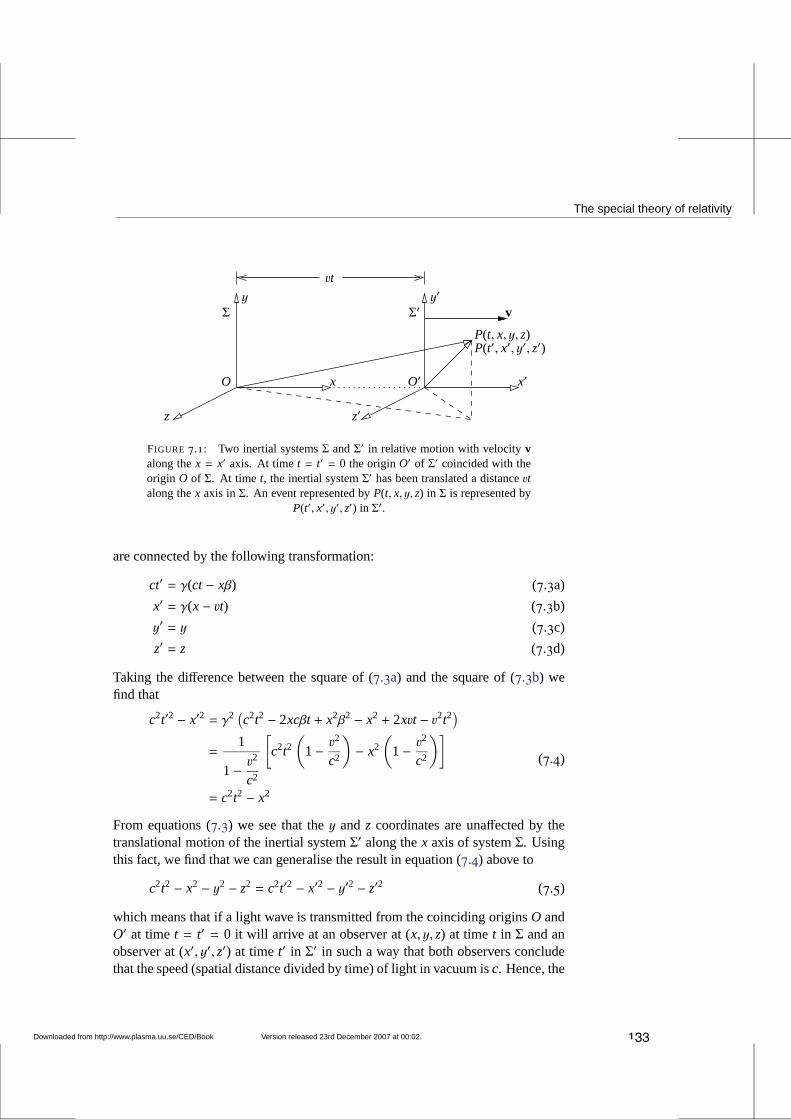
The special theory of relativity
v
P(t′, x′, y′, z′)
vt
P(t, x, y, z)
z′
x x′
z
O O′
Σ Σ′y y′
FIGURE 7.1: Two inertial systemsΣ andΣ′ in relative motion with velocityvalong thex = x′ axis. At timet = t′ = 0 the originO′ of Σ′ coincided with theorigin O of Σ. At time t, the inertial systemΣ′ has been translated a distancevtalong thex axis inΣ. An event represented byP(t, x, y, z) in Σ is represented by
P(t′, x′, y′, z′) in Σ′.
are connected by the following transformation:
ct′ = γ(ct− xβ) (7.3a)
x′ = γ(x− vt) (7.3b)
y′ = y (7.3c)
z′ = z (7.3d)
Taking the difference between the square of (7.3a) and the square of (7.3b) wefind that
c2t′2 − x′2 = γ2(c2t2 − 2xcβt + x2β2 − x2 + 2xvt − v2t2
)
=1
1− v2
c2
[
c2t2(
1− v2
c2
)
− x2
(
1− v2
c2
)]
= c2t2 − x2
(7.4)
From equations (7.3) we see that they andz coordinates are unaffected by thetranslational motion of the inertial systemΣ′ along thex axis of systemΣ. Usingthis fact, we find that we can generalise the result in equation (7.4) above to
c2t2 − x2 − y2 − z2 = c2t′2 − x′2 − y′2 − z′2 (7.5)
which means that if a light wave is transmitted from the coinciding originsO andO′ at timet = t′ = 0 it will arrive at an observer at (x, y, z) at timet in Σ and anobserver at (x′, y′, z′) at timet′ in Σ′ in such a way that both observers concludethat the speed (spatial distance divided by time) of light invacuum isc. Hence, the
Downloaded from http://www.plasma.uu.se/CED/Book Version released 23rd December 2007 at 00:02. 133
7. Relativistic Electrodynamics
speed of light inΣ andΣ′ is the same. A linear coordinate transformation whichhas this property is called a (homogeneous)Lorentz transformation.
7.1.2 Lorentz spaceLet us introduce an ordered quadruple of real numbers, enumerated with the helpof upper indicesµ = 0, 1, 2, 3, where the zeroth component isct (c is the speedof light andt is time), and the remaining components are the components oftheordinaryR3 radius vectorx defined in equation (M.1) on page180:
xµ = (x0, x1, x2, x3) = (ct, x, y, z) ≡ (ct, x) (7.6)
We want to interpret this quadruplexµ as (the component form of) aradius four-vectorin a real, linear,four-dimensional vector space.2 We require that this four-dimensional space be aRiemannian space, i.e., a metric space where a ‘distance’and a scalar product are defined. In this space we therefore define ametric tensor,also known as thefundamental tensor, which we denote bygµν.
Radius four-vector in contravariant and covariant form
The radius four-vectorxµ = (x0, x1, x2, x3) = (ct, x), as defined in equation (7.6)above, is, by definition, the prototype of acontravariant vector(or, more accu-rately, a vector incontravariant component form). To every such vector thereexists adual vector. The vector dual toxµ is thecovariant vector xµ, obtained as
xµ = gµνxν (7.7)
where the upper indexµ in xµ is summed over and is therefore adummy indexand may be replaced by another dummy indexν This summation process is anexample ofindex contractionand is often referred to asindex lowering.
Scalar product and norm
The scalar product ofxµ with itself in a Riemannian space is defined as
gµνxνxµ = xµxµ (7.8)
2The British mathematician and philosopher Alfred North Whitehead writes in his bookThe Conceptof Nature[13]:
‘I regret that it has been necessary for me in this lecture to administer a large dose offour-dimensional geometry. I do not apologise, because I amreally not responsible for thefact that nature in its most fundamental aspect is four-dimensional. Things are what theyare. . . .’
134 Version released 23rd December 2007 at 00:02. Downloaded from http://www.plasma.uu.se/CED/Book
The special theory of relativity
This scalar product acts as an invariant ‘distance’, ornorm, in this space.To describe the physical property of Lorentz transformation invariance, de-
scribed by equation (7.5) on page133, in mathematical language it is convenientto perceive it as the manifestation of the conservation of the norm in a 4D Rieman-nian space. Then the explicit expression for the scalar product of xµ with itself inthis space must be
xµxµ = c2t2 − x2 − y2 − z2 (7.9)
We notice that our space will have anindefinite normwhich means that we dealwith a non-Euclidean space. We call the four-dimensional space (orspace-time)with this propertyLorentz spaceand denote itL4. A corresponding real, linear 4Dspace with apositive definite normwhich is conserved during ordinary rotationsis aEuclidean vector space. We denote such a spaceR4.
Metric tensor
By choosing the metric tensor inL4 as
gµν =
1 if µ = ν = 0
−1 if µ = ν = i = j = 1, 2, 3
0 if µ , ν
(7.10)
or, in matrix notation,
(gµν) =
1 0 0 00 −1 0 00 0 −1 00 0 0 −1
(7.11)
i.e., a matrix with a main diagonal that has the sign sequence, orsignature,+,−,−,−, the index lowering operation in our chosen flat 4D space becomesnearly trivial:
xµ = gµνxν = (ct,−x) (7.12)
Using matrix algebra, this can be written
x0
x1
x2
x3
=
1 0 0 00 −1 0 00 0 −1 00 0 0 −1
x0
x1
x2
x3
=
x0
−x1
−x2
−x3
(7.13)
Hence, if the metric tensor is defined according to expression (7.10) above the co-variant radius four-vectorxµ is obtained from the contravariant radius four-vector
Downloaded from http://www.plasma.uu.se/CED/Book Version released 23rd December 2007 at 00:02. 135
7. Relativistic Electrodynamics
xµ simply by changing the sign of the last three components. These componentsare referred to as thespace components; the zeroth component is referred to as thetime component.
As we see, for this particular choice of metric, the scalar product of xµ withitself becomes
xµxµ = (ct, x) · (ct,−x) = c2t2 − x2 − y2 − z2 (7.14)
which indeed is the desired Lorentz transformation invariance as required by equa-tion (7.9) on page135. Without changing the physics, one can alternatively choosea signature−,+,+,+. The latter has the advantage that the transition from 3Dto 4D becomes smooth, while it will introduce some annoying minus signs in thetheory. In current physics literature, the signature+,−,−,− seems to be the mostcommonly used one.
TheL4 metric tensor equation (7.10) on page135 has a number of interestingproperties: firstly, we see that this tensor has a trace Tr
(gµν)= −2 whereas inR4,
as in any vector space with definite norm, the trace equals thespace dimension-ality. Secondly, we find, after trivial algebra, that the following relations betweenthe contravariant, covariant and mixed forms of the metric tensor hold:
gµν = gνµ (7.15a)
gµν = gµν (7.15b)
gνκgκµ = gµν = δ
µν (7.15c)
gνκgκµ = gνµ = δ
νµ (7.15d)
Here we have introduced the 4D version of the Kronecker deltaδµν , a mixed four-
tensor of rank 2 which fulfils
δµν = δνµ =
1 if µ = ν
0 if µ , ν(7.16)
Invariant line element and proper time
Thedifferential distanceds between the two pointsxµ andxµ + dxµ in L4 can becalculated from theRiemannian metric, given by thequadratic differential form
ds2 = gµνdxνdxµ = dxµdxµ = (dx0)2 − (dx1)2 − (dx2)2 − (dx3)2 (7.17)
where the metric tensor is as in equation (7.10) on page135. As we see, thisform is indefiniteas expected for a non-Euclidean space. The square root of this
136 Version released 23rd December 2007 at 00:02. Downloaded from http://www.plasma.uu.se/CED/Book
The special theory of relativity
expression is theinvariant line element
ds= cdt
√√√√1− 1
c2
[(dxdt
1)2
+
(dxdt
2)2
+
(dxdt
3)2]
= cdt
√
1− 1c2
[(vx)2 + (vy)2 + (vz)2
]= cdt
√
1− v2
c2
= cdt√
1− β2 = cdtγ= cdτ
(7.18)
where we introduced
dτ = dt/γ (7.19)
Since dτ measures the time when no spatial changes are present, it is called theproper time.
Expressing the property of the Lorentz transformation described by equa-tions (7.5) on page133 in terms of the differential interval ds and comparingwith equation (7.17) on page136, we find that
ds2 = c2dt2 − dx2 − dy2 − dz2 (7.20)
is invariant,i.e., remains unchanged, during a Lorentz transformation. Conversely,we may say that every coordinate transformation which preserves this differentialinterval is a Lorentz transformation.
If in some inertial system
dx2 + dy2 + dz2 < c2dt2 (7.21)
ds is atime-like interval, but if
dx2 + dy2 + dz2 > c2dt2 (7.22)
ds is aspace-like interval, whereas
dx2 + dy2 + dz2 = c2dt2 (7.23)
is a light-like interval; we may also say that in this case we are on thelight cone.A vector which has a light-like interval is called anull vector. The time-like,space-like or light-like aspects of an interval ds are invariant under a Lorentztransformation.I.e., it is not possible to change a time-like interval into a space-like one orvice versavia a Lorentz transformation.
Downloaded from http://www.plasma.uu.se/CED/Book Version released 23rd December 2007 at 00:02. 137
7. Relativistic Electrodynamics
Four-vector fields
Any quantity which relative to any coordinate system has a quadruple of realnumbers and transforms in the same way as the radius four-vector xµ does, iscalled afour-vector. In analogy with the notation for the radius four-vector weintroduce the notationaµ = (a0, a) for a generalcontravariant four-vector fieldinL4 and find that the ‘lowering of index’ rule, formula (7.7) on page134, for suchan arbitrary four-vector yields the dualcovariant four-vector field
aµ(xκ) = gµνa
ν(xκ) = (a0(xκ),−a(xκ)) (7.24)
The scalar product between this four-vector field and another onebµ(xκ) is
gµνaν(xκ)bµ(xκ) = (a0,−a) · (b0, b) = a0b0 − a · b (7.25)
which is ascalar field, i.e., an invariant scalar quantityα(xκ) which depends ontime and space, as described byxκ = (ct, x, y, z).
The Lorentz transformation matrix
Introducing the transformation matrix
(Λµν
)=
γ −βγ 0 0−βγ γ 0 0
0 0 1 00 0 0 1
(7.26)
the linear Lorentz transformation (7.3) on page133, i.e., the coordinate transfor-mationxµ → x′µ = x′µ(x0, x1, x2, x3), from one inertial systemΣ to another inertialsystemΣ′ in the standard configuration, can be written
x′µ = Λµνxν (7.27)
The Lorentz group
It is easy to show, by means of direct algebra, that two successive Lorentz transfor-mations of the type in equation (7.27) above, and defined by the speed parametersβ1 andβ2, respectively, correspond to a single transformation withspeed parame-ter
β =β1 + β2
1+ β1β2(7.28)
This means that the nonempty set of Lorentz transformationsconstitutes aclosedalgebraic structurewith a binary operation which isassociative. Furthermore,
138 Version released 23rd December 2007 at 00:02. Downloaded from http://www.plasma.uu.se/CED/Book
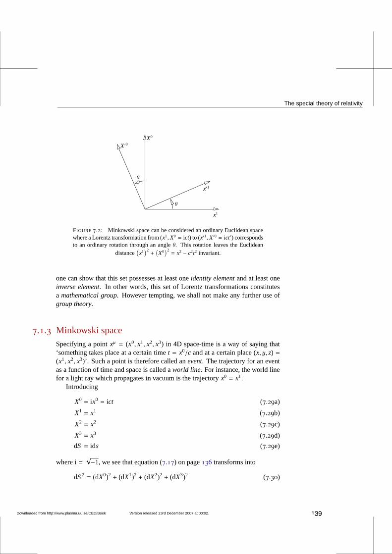
The special theory of relativity
θ
θ
X′0
x′1
x1
X0
FIGURE 7.2: Minkowski space can be considered an ordinary Euclidean spacewhere a Lorentz transformation from (x1,X0 = ict) to (x′1,X′0 = ict′) correspondsto an ordinary rotation through an angleθ. This rotation leaves the Euclidean
distance(x1)2+(X0)2= x2 − c2t2 invariant.
one can show that this set possesses at least oneidentity elementand at least oneinverse element. In other words, this set of Lorentz transformations constitutesa mathematical group. However tempting, we shall not make any further use ofgroup theory.
7.1.3 Minkowski spaceSpecifying a pointxµ = (x0, x1, x2, x3) in 4D space-time is a way of saying that‘something takes place at a certain timet = x0/c and at a certain place (x, y, z) =(x1, x2, x3)’. Such a point is therefore called anevent. The trajectory for an eventas a function of time and space is called aworld line. For instance, the world linefor a light ray which propagates in vacuum is the trajectoryx0 = x1.
Introducing
X0 = ix0 = ict (7.29a)
X1 = x1 (7.29b)
X2 = x2 (7.29c)
X3 = x3 (7.29d)
dS = ids (7.29e)
where i=√−1, we see that equation (7.17) on page136 transforms into
dS2 = (dX0)2 + (dX1)2 + (dX2)2 + (dX3)2 (7.30)
Downloaded from http://www.plasma.uu.se/CED/Book Version released 23rd December 2007 at 00:02. 139
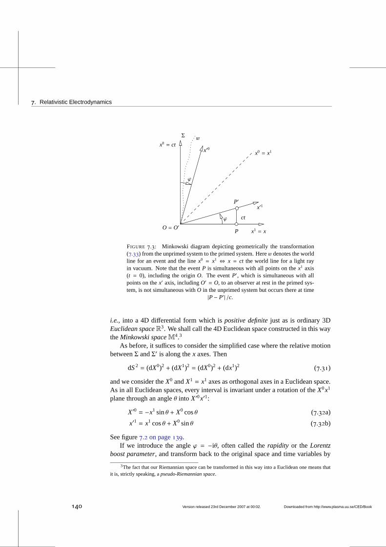
7. Relativistic Electrodynamics
x0 = ct
ct
x′1
x′0
x1 = xO = O′
ϕ
P
P′
ϕ
x0 = x1
wΣ
FIGURE 7.3: Minkowski diagram depicting geometrically the transformation(7.33) from the unprimed system to the primed system. Herew denotes the worldline for an event and the linex0 = x1 ⇔ x = ct the world line for a light rayin vacuum. Note that the eventP is simultaneous with all points on thex1 axis(t = 0), including the originO. The eventP′, which is simultaneous with allpoints on thex′ axis, includingO′ = O, to an observer at rest in the primed sys-tem, is not simultaneous withO in the unprimed system but occurs there at time
|P− P′| /c.
i.e., into a 4D differential form which ispositive definitejust as is ordinary 3DEuclidean spaceR3. We shall call the 4D Euclidean space constructed in this waytheMinkowski spaceM4.3
As before, it suffices to consider the simplified case where the relative motionbetweenΣ andΣ′ is along thex axes. Then
dS2 = (dX0)2 + (dX1)2 = (dX0)2 + (dx1)2 (7.31)
and we consider theX0 andX1 = x1 axes as orthogonal axes in a Euclidean space.As in all Euclidean spaces, every interval is invariant under a rotation of theX0x1
plane through an angleθ into X′0x′1:
X′0 = −x1 sinθ + X0 cosθ (7.32a)
x′1 = x1 cosθ + X0 sinθ (7.32b)
See figure7.2 on page139.If we introduce the angleϕ = −iθ, often called therapidity or the Lorentz
boost parameter, and transform back to the original space and time variablesby
3The fact that our Riemannian space can be transformed in thisway into a Euclidean one means thatit is, strictly speaking, apseudo-Riemannian space.
140 Version released 23rd December 2007 at 00:02. Downloaded from http://www.plasma.uu.se/CED/Book
Covariant classical mechanics
using equation (7.29) on page139 backwards, we obtain
ct′ = −xsinhϕ + ctcoshϕ (7.33a)
x′ = xcoshϕ − ctsinhϕ (7.33b)
which are identical to the transformation equations (7.3) on page133 if we let
sinhϕ = γβ (7.34a)
coshϕ = γ (7.34b)
tanhϕ = β (7.34c)
It is therefore possible to envisage the Lorentz transformation as an ‘ordinary’rotation in the 4D Euclidean spaceM4. Such a rotation inM4 corresponds to acoordinate change inL4 as depicted in figure7.3 on page140. equation (7.28)on page138 for successive Lorentz transformation then corresponds tothe tanhaddition formula
tanh(ϕ1 + ϕ2) =tanhϕ1 + tanhϕ2
1+ tanhϕ1 tanhϕ2(7.35)
The use of ict andM4, which leads to the interpretation of the Lorentz trans-formation as an ‘ordinary’ rotation, may, at best, be illustrative, but is not veryphysical. Besides, if we leave the flatL4 space and enter the curved space ofgeneral relativity, the ‘ict’ trick will turn out to be an impasse. Let us thereforeimmediately return toL4 where all components are real valued.
7.2 Covariant classical mechanicsThe invariance of the differential ‘distance’ ds in L4, and the associated differ-ential proper time dτ [see equation (7.18) on page137] allows us to define thefour-velocity
uµ =dxdτ
µ
= γ(c, v) =
c
√
1− v2
c2
,v
√
1− v2
c2
= (u0, u) (7.36)
which, when multiplied with the scalar invariantm0 yields thefour-momentum
pµ = m0dxdτ
µ
= m0γ(c, v) =
m0c
√
1− v2
c2
,m0v
√
1− v2
c2
= (p0, p) (7.37)
Downloaded from http://www.plasma.uu.se/CED/Book Version released 23rd December 2007 at 00:02. 141
7. Relativistic Electrodynamics
From this we see that we can write
p = mv (7.38)
where
m= γm0 =m0
√
1− v2
c2
(7.39)
We can interpret this such that the Lorentz covariance implies that the mass-liketerm in the ordinary 3D linear momentum is not invariant. A better way to lookat this is thatp = mv = γm0v is the covariantly correct expression for the kineticthree-momentum.
Multiplying the zeroth (time) component of the four-momentum pµ with thescalar invariantc, we obtain
cp0 = γm0c2 =
m0c2
√
1− v2
c2
= mc2 (7.40)
Since this component has the dimension of energy and is the result of a covariantdescription of the motion of a particle with its kinetic momentum described bythe spatial components of the four-momentum, equation (7.37) on page141, weinterpretcp0 as the total energyE. Hence,
cpµ = (cp0, cp) = (E, cp) (7.41)
Scalar multiplying this four-vector with itself, we obtain
cpµcpµ = c2gµνpνpµ = c2[(p0)2 − (p1)2 − (p2)2 − (p3)2]
= (E,−cp) · (E, cp) = E2 − c2p2
=(m0c2)2
1− v2
c2
(
1− v2
c2
)
= (m0c2)2
(7.42)
Since this is an invariant, this equation holds in any inertial frame, particularly inthe frame wherep = 0 and there we have
E = m0c2 (7.43)
This is probably the most famous formula in physics history.
142 Version released 23rd December 2007 at 00:02. Downloaded from http://www.plasma.uu.se/CED/Book
Covariant classical electrodynamics
7.3 Covariant classical electrodynamicsLet us consider a charge density which in its rest inertial system is denoted byρ0.The four-vector (in contravariant component form)
jµ = ρ0dxµ
dτ= ρ0u
µ = ρ0γ(c, v) = (ρc, ρv) (7.44)
where we introduced
ρ = γρ0 (7.45)
is called thefour-current.The contravariant form of the four-del operator∂µ = ∂/∂xµ is defined in
equation (M.37) on page187 and its covariant counterpart∂µ = ∂/∂xµ in equa-tion (M.38) on page187, respectively. As is shown in exampleM.5 on page197,thed’Alembert operatoris the scalar product of the four-del with itself:
2 = ∂µ∂µ = ∂µ∂µ =
1c2
∂2
∂t2− ∇2 (7.46)
Since it has the characteristics of a four-scalar, the d’Alembert operator is invariantand, hence, the homogeneous wave equation2 f (t, x) = 0 is Lorentz covariant.
7.3.1 The four-potentialIf we introduce thefour-potential
Aµ =
(φ
c,A)
(7.47)
whereφ is the scalar potential andA the vector potential, defined in section3.3 on page40,we can write the uncoupled inhomogeneous wave equations, equations (3.16) onpage43, in the following compact (and covariant) way:
2Aµ = µ0 jµ (7.48)
With the help of the above, we can formulate our electrodynamic equationscovariantly. For instance, the covariant form of theequation of continuity, equa-tion (1.23) on page10 is
∂µ jµ = 0 (7.49)
and theLorenz-Lorentz gauge condition, equation (3.15) on page43, can be writ-ten
∂µAµ = 0 (7.50)
Downloaded from http://www.plasma.uu.se/CED/Book Version released 23rd December 2007 at 00:02. 143
7. Relativistic Electrodynamics
The gauge transformations (3.11) on page42 in covariant form are
Aµ 7→ A′µ = Aµ + ∂µΓ(xν) (7.51)
If only one dimension Lorentz contracts (for instance, due to relative motionalong thex direction), a 3D spatial volume element transforms according to
dV = d3x =1γ
dV0 = dV0
√
1− β2 = dV0
√
1− v2
c2(7.52)
where dV0 denotes the volume element as measured in the rest system, then fromequation (7.45) on page143 we see that
ρdV = ρ0dV0 (7.53)
i.e., the charge in a given volume is conserved. We can therefore conclude thatthe elementary charge is a universal constant.
7.3.2 The Liénard-Wiechert potentialsLet us now solve the the inhomogeneous wave equations (3.16) on page43 invacuum for the case of a well-localised chargeq′ at a source point defined by theradius four-vectorx′µ ≡ (x′0 = ct′, x′1, x′2, x′3). The field point (observation point)is denoted by the radius four-vectorxµ = (x0 = ct, x1, x2, x3).
In the rest system we know that the solution is simply
(Aµ)0 =
(φ
c,A)
v=0=
(q′
4πε0
1c |x − x′|0
, 0)
(7.54)
where|x − x′|0 is the usual distance from the source point to the field point,eval-uated in the rest system (signified by the index ‘0’).
Let us introduce the relative radius four-vector between the source point andthe field point:
Rµ = xµ − x′µ = (c(t − t′), x − x′) (7.55)
Scalar multiplying this relative four-vector with itself,we obtain
RµRµ = (c(t − t′), x − x′) · (c(t − t′),−(x − x′)) = c2(t − t′)2 −∣∣x − x′
∣∣2
(7.56)
We know that in vacuum the signal (field) from the chargeq′ at x′µ propagatesto xµ with the speed of lightc so that
∣∣x − x′
∣∣ = c(t − t′) (7.57)
144 Version released 23rd December 2007 at 00:02. Downloaded from http://www.plasma.uu.se/CED/Book
Covariant classical electrodynamics
Inserting this into equation (7.56) on page144, we see that
RµRµ = 0 (7.58)
or that equation (7.55) on page144 can be written
Rµ = (∣∣x − x′
∣∣ , x − x′) (7.59)
Now we want to find the correspondence to the rest system solution, equa-tion (7.54) on page144, in an arbitrary inertial system. We note from equa-tion (7.36) on page141 that in the rest system
(uµ)0 =
c
√
1− v2
c2
,v
√
1− v2
c2
v=0
= (c, 0) (7.60)
and
(Rµ)0 = (∣∣x − x′
∣∣ , x − x′)0 = (
∣∣x − x′
∣∣0 , (x − x′)0) (7.61)
As all scalar products,uµRµ is invariant, which means that we can evaluate itin any inertial system and it will have the same value in all other inertial systems.If we evaluate it in the rest system the result is:
uµRµ =(uµRµ
)
0 = (uµ)0(Rµ)0
= (c, 0) · (∣∣x − x′
∣∣0 ,−(x − x′)0) = c
∣∣x − x′
∣∣0
(7.62)
We therefore see that the expression
Aµ =q′
4πε0
uµ
cuνRν
(7.63)
subject to the conditionRµRµ = 0 has the proper transformation properties (propertensor form) and reduces, in the rest system, to the solutionequation (7.54) onpage144. It is therefore the correct solution, valid in any inertialsystem.
According to equation (7.36) on page141 and equation (7.59)
uνRν = γ(c, v) ·(∣∣x − x′
∣∣ ,−(x − x′)
)= γ
(c∣∣x − x′
∣∣ − v · (x − x′)
)(7.64)
Generalising expression (7.1) on page132 to vector form:
β = β vdef≡ v
c(7.65)
and introducing
sdef≡∣∣x − x′
∣∣ − v · (x − x′)
c≡∣∣x − x′
∣∣ − β · (x − x′) (7.66)
Downloaded from http://www.plasma.uu.se/CED/Book Version released 23rd December 2007 at 00:02. 145
7. Relativistic Electrodynamics
we can write
uνRν = γcs (7.67)
and
uµ
cuνRν
=
(1cs,
vc2s
)
(7.68)
from which we see that the solution (7.63) can be written
Aµ(xκ) =q′
4πε0
(1cs,
vc2s
)
=
(φ
c,A)
(7.69)
where in the last step the definition of the four-potential, equation (7.47) on page143,was used. Writing the solution in the ordinary 3D way, we conclude that for a verylocalised charge volume, moving relative an observer with avelocity v, the scalarand vector potentials are given by the expressions
φ(t, x) =q′
4πε0
1s=
q′
4πε0
1|x − x′| − β · (x − x′)
(7.70a)
A(t, x) =q′
4πε0c2
vs=
q′
4πε0c2
v|x − x′| − β · (x − x′)
(7.70b)
These potentials are theLiénard-Wiechert potentialsthat we derived in a morecomplicated and restricted way in subsection6.3.1 on page94.
7.3.3 The electromagnetic field tensorConsider a vectorial (cross) productc between two ordinary vectorsa andb:
c = a× b = ǫi jkaibj xk
= (a2b3 − a3b2)x1 + (a3b1 − a1b3)x2 + (a1b2 − a2b1)x3(7.71)
We notice that thekth component of the vectorc can be represented as
ck = aibj − ajbi = ci j = −cji , i, j , k (7.72)
In other words, thepseudovectorc = a×b can be considered as anantisymmetrictensorof rank two. The same is true for the curl operator∇× operating on a polarvector. For instance, the Maxwell equation
∇ × E = −∂B∂t
(7.73)
146 Version released 23rd December 2007 at 00:02. Downloaded from http://www.plasma.uu.se/CED/Book
Covariant classical electrodynamics
can in this tensor notation be written
∂E j
∂xi− ∂Ei
∂x j= −∂Bi j
∂t(7.74)
We know from chapter3 that the fields can be derived from the electromag-netic potentials in the following way:
B = ∇ × A (7.75a)
E = −∇φ − ∂A∂t
(7.75b)
In component form, this can be written
Bi j =∂A j
∂xi− ∂Ai
∂x j= ∂iA j − ∂ jAi (7.76a)
Ei = −∂φ
∂xi− ∂Ai
∂t= −∂iφ − ∂tAi (7.76b)
From this, we notice the clear difference between theaxial vector(pseudovector)B and thepolar vector(‘ordinary vector’)E.
Our goal is to express the electric and magnetic fields in a tensor form wherethe components are functions of the covariant form of the four-potential, equa-tion (7.47) on page143:
Aµ =
(φ
c,A)
(7.77)
Inspection of (7.77) and equation (7.76) above makes it natural to define the four-tensor
Fµν =∂Aν
∂xµ− ∂Aµ
∂xν= ∂µAν − ∂νAµ (7.78)
This anti-symmetric (skew-symmetric), four-tensor of rank 2 is called theelectro-magnetic field tensor. In matrix representation, thecontravariant field tensorcanbe written
(Fµν) =
0 −Ex/c −Ey/c −Ez/cEx/c 0 −Bz ByEy/c Bz 0 −Bx
Ez/c −By Bx 0
(7.79)
We note that the field tensor is a sort of four-dimensional curl of the four-potentialvectorAµ.
Downloaded from http://www.plasma.uu.se/CED/Book Version released 23rd December 2007 at 00:02. 147
7. Relativistic Electrodynamics
Thecovariant field tensoris obtained from the contravariant field tensor in theusual manner by index lowering
Fµν = gµκgνλFκλ = ∂µAν − ∂νAµ (7.80)
which in matrix representation becomes
(Fµν
)=
0 Ex/c Ey/c Ez/c−Ex/c 0 −Bz By−Ey/c Bz 0 −Bx
−Ez/c −By Bx 0
(7.81)
Comparing formula (7.81) with formula (7.79) on page147 we see that the co-variant field tensor is obtained from the contravariant one by a transformationE→ −E.
That the two Maxwell source equations can be written
∂µFµν = µ0 jν (7.82)
is immediately observed by explicitly solving this covariant equation. Settingν = 0, corresponding to the first/leftmost column in the matrix representation ofthe covariant component form of the electromagnetic field tensor,Fµν, i.e., equa-tion (7.79) on page147, we see that
∂F00
∂x0+∂F10
∂x1+∂F20
∂x2+∂F30
∂x3= 0+
1c
(∂Ex
∂x+∂Ey
∂y+∂Ez
∂z
)
=1c∇ · E = µ0 j0 = µ0cρ
(7.83)
or, equivalently (recalling thatε0µ0 = 1/c2),
∇ · E = ρ
ε0(7.84)
which we recognise at the Maxwell source equation for the electric field, equa-tion (1.45a) on page15.
Forν = 1 (the second column in equation (7.79) on page147), equation (7.82)above yields
∂F01
∂x0+∂F11
∂x1+∂F21
∂x2+∂F31
∂x3= − 1
c2
∂Ex
∂t+ 0+
∂Bz
∂y− ∂By
∂z= µ0 j1 = µ0ρvx
(7.85)
This result can be rewritten as
∂Bz
∂y− ∂By
∂z− ε0µ0
∂Ex
∂t= µ0 jx (7.86)
148 Version released 23rd December 2007 at 00:02. Downloaded from http://www.plasma.uu.se/CED/Book
Covariant classical electrodynamics
or, equivalently, as
(∇ × B)x = µ0 jx + ε0µ0∂Ex
∂t(7.87)
and similarly forν = 2, 3. In summary, we can write the result in three-vectorform as
∇ × B = µ0j (t, x) + ε0µ0∂E∂t
(7.88)
which we recognise as the Maxwell source equation for the magnetic field, equa-tion (1.45d) on page15.
With the help of the fully antisymmetric rank-4 pseudotensor
ǫµνκλ =
1 if µ, ν, κ, λ is anevenpermutation of 0,1,2,3
0 if at least two ofµ, ν, κ, λ are equal
−1 if µ, ν, κ, λ is anoddpermutation of 0,1,2,3
(7.89)
which can be viewed as a generalisation of the Levi-Civita tensor, formula (M.18)on page183, we can introduce thedual electromagnetic tensor
⋆Fµν = ǫµνκλFκλ (7.90)
In matrix form the dual field tensor is
(⋆Fµν
)=
0 −cBx −cBy −cBz
cBx 0 Ez −Ey
cBy −Ez 0 Ex
cBz Ey −Ex 0
(7.91)
i.e., the dual field tensor is obtained from the ordinary field tensor by thedualitytransformationE→ c2B andB→ −E.
The covariant form of the two Maxwell field equations
∇ × E = −∂B∂t
(7.92)
∇ · B = 0 (7.93)
can then be written
∂µ⋆Fµν = 0 (7.94)
Explicit evaluation shows that this corresponds to (no summation!)
∂κFµν + ∂µFνκ + ∂νFκµ = 0 (7.95)
Downloaded from http://www.plasma.uu.se/CED/Book Version released 23rd December 2007 at 00:02. 149

7. Relativistic Electrodynamics
sometimes referred to as theJacobi identity. Hence, equation (7.82) on page148and equation (7.95) on page149 constitute Maxwell’s equations in four-dimensionalformalism.
It is interesting to note that equation (7.82) on page148 and
∂µ⋆Fµν = µ0 jνm (7.96)
where jm is the magnetic four-current, represent the covariant form of Dirac’ssymmetrised Maxwell equations (1.50) on page16.
7.4 Bibliography[1] J. AHARONI, The Special Theory of Relativity, second, revised ed., Dover Publica-
tions, Inc., New York, 1985, ISBN 0-486-64870-2.
[2] A. O. BARUT, Electrodynamics and Classical Theory of Fields and Particles, Dover Pub-lications, Inc., New York, NY, 1980, ISBN 0-486-64038-8.
[3] R. BECKER, Electromagnetic Fields and Interactions, Dover Publications, Inc.,New York, NY, 1982, ISBN 0-486-64290-9.
[4] D. BOHM, The Special Theory of Relativity, Routledge, New York, NY, 1996, ISBN 0-415-14809-X.131
[5] W. T. GRANDY, Introduction to Electrodynamics and Radiation, Academic Press,New York and London, 1970, ISBN 0-12-295250-2.
[6] L. D. LANDAU AND E. M. LIFSHITZ, The Classical Theory of Fields, fourth revisedEnglish ed., vol. 2 ofCourse of Theoretical Physics, Pergamon Press, Ltd., Oxford . . . ,1975, ISBN 0-08-025072-6.
[7] F. E. LOW, Classical Field Theory, John Wiley & Sons, Inc., New York, NY . . . , 1997,ISBN 0-471-59551-9.
[8] H. MUIRHEAD, The Special Theory of Relativity, The Macmillan Press Ltd., London,Beccles and Colchester, 1973, ISBN 333-12845-1.
[9] C. MØLLER, The Theory of Relativity, second ed., Oxford University Press, Glasgow . . . ,1972.
[10] W. K. H. PANOFSKY AND M. PHILLIPS, Classical Electricity and Magnetism, second ed.,Addison-Wesley Publishing Company, Inc., Reading, MA . . . ,1962, ISBN 0-201-05702-6.
[11] J. J. SAKURAI , Advanced Quantum Mechanics, Addison-Wesley Publishing Com-pany, Inc., Reading, MA . . . , 1967, ISBN 0-201-06710-2.
150 Version released 23rd December 2007 at 00:02. Downloaded from http://www.plasma.uu.se/CED/Book
Bibliography
[12] B. SPAIN, Tensor Calculus, third ed., Oliver and Boyd, Ltd., Edinburgh and London,1965, ISBN 05-001331-9.
[13] A. N. WHITEHEAD, Concept of Nature, Cambridge University Press, Cambridge . . . ,1920, ISBN 0-521-09245-0.134
Downloaded from http://www.plasma.uu.se/CED/Book Version released 23rd December 2007 at 00:02. 151

Downloaded from http://www.plasma.uu.se/CED/Book Version released 23rd December 2007 at 00:02.
8ELECTROMAGNETIC FIELDS AND
PARTICLES
In previous chapters, we calculated the electromagnetic fields and potentials fromarbitrary, but prescribed distributions of charges and currents. In this chapter westudy the general problem of interaction between electric and magnetic fields andelectrically charged particles. The analysis is based on Lagrangian and Hamil-tonian methods, is fully covariant, and yields results which are relativisticallycorrect.
8.1 Charged particles in an electromagnetic fieldWe first establish a relativistically correct theory describing the motion of chargedparticles in prescribed electric and magnetic fields. From these equations we maythen calculate the charged particle dynamics in the most general case.
8.1.1 Covariant equations of motionWe will show that for our problem we can derive the correct equations of mo-tion by using in four-dimensionalL4 a function with similar properties as a La-grange function in 3D and then apply a variational principle. We will also showthat we can find a Hamiltonian-type function in 4D and solve the correspondingHamilton-type equations to obtain the correct covariant formulation of classicalelectrodynamics.
153
8. Electromagnetic Fields and Particles
Lagrangian formalism
Let us now introduce a generalised action
S4 =
∫
L4(xµ, uµ) dτ (8.1)
where dτ is the proper time defined via equation (7.18) on page137, andL4 actsas a kind of generalisation to the common 3D Lagrangian so that the variationalprinciple
δS4 = δ
∫ τ1
τ0
L4(xµ, uµ) dτ = 0 (8.2)
with fixed endpointsτ0, τ1 is fulfilled. We require thatL4 is a scalar invariantwhich does not contain higher than the second power of the four-velocity uµ inorder that the equations of motion be linear.
According to formula (M.48) on page189 the ordinary 3D Lagrangian is thedifference between the kinetic and potential energies. A free particle has onlykinetic energy. If the particle mass ism0 then in 3D the kinetic energy ism0v
2/2.This suggests that in 4D the Lagrangian for a free particle should be
Lfree4 =
12
m0uµuµ (8.3)
For an interaction with the electromagnetic field we can introduce the interactionwith the help of the four-potential given by equation (7.77) on page147 in thefollowing way
L4 =12
m0uµuµ + quµA
µ(xν) (8.4)
We call this thefour-Lagrangianand shall now show how this function, togetherwith the variation principle, formula (8.2) above, yields covariant results whichare physically correct.
The variation principle (8.2) with the 4D Lagrangian (8.4) inserted, leads to
δS4 = δ
∫ τ1
τ0
(m0
2uµuµ + quµAµ(x
ν))
dτ
=
∫ τ1
τ0
[m0
2∂(uµuµ)∂uµ
δuµ + q
(
Aµδuµ + uµ
∂Aµ
∂xνδxν)]
dτ
=
∫ τ1
τ0
[m0uµδu
µ + q(Aµδu
µ + uµ∂νAµδxν)]
dτ = 0
(8.5)
According to equation (7.36) on page141, the four-velocity is
uµ =dxdτ
µ
(8.6)
154 Version released 23rd December 2007 at 00:02. Downloaded from http://www.plasma.uu.se/CED/Book
Charged particles in an electromagnetic field
which means that we can write the variation ofuµ as a total derivative with respectto τ :
δuµ = δ
(dxdτ
µ)
=ddτ
(δxµ) (8.7)
Inserting this into the first two terms in the last integral inequation (8.5) onpage154, we obtain
δS4 =
∫ τ1
τ0
(
m0uµddτ
(δxµ) + qAµddτ
(δxµ) + quµ∂νAµδxν)
dτ (8.8)
Partial integration in the two first terms in the right hand member of (8.8) gives
δS4 =
∫ τ1
τ0
(
−m0duµdτ
δxµ − qdAµ
dτδxµ + quµ∂νAµδxν
)
dτ (8.9)
where the integrated parts do not contribute since the variations at the endpointsvanish. A change of irrelevant summation index fromµ to ν in the first two termsof the right hand member of (8.9) yields, after moving the ensuing common factorδxν outside the parenthesis, the following expression:
δS4 =
∫ τ1
τ0
(
−m0duνdτ− q
dAν
dτ+ quµ∂νAµ
)
δxν dτ (8.10)
Applying well-known rules of differentiation and the expression (7.36) for thefour-velocity, we can express dAν/dτ as follows:
dAν
dτ=∂Aν
∂xµdxµ
dτ= ∂µAνu
µ (8.11)
By inserting this expression (8.11) into the second term in right-hand member ofequation (8.10), and noting the common factorquµ of the resulting term and thelast term, we obtain the final variational principle expression
δS4 =
∫ τ1
τ0
[
−m0duνdτ+ quµ
(∂νAµ − ∂µAν
)]
δxν dτ (8.12)
Since, according to the variational principle, this expression shall vanish andδxν
is arbitrary between the fixed end pointsτ0 andτ1, the expression inside[ ]
in theintegrand in the right hand member of equation (8.12) above must vanish. In otherwords, we have found an equation of motion for a charged particle in a prescribedelectromagnetic field:
m0duνdτ= quµ
(∂νAµ − ∂µAν
)(8.13)
Downloaded from http://www.plasma.uu.se/CED/Book Version released 23rd December 2007 at 00:02. 155
8. Electromagnetic Fields and Particles
With the help of formula (7.80) on page148 for the covariant component form ofthe field tensor, we can express this equation in terms of the electromagnetic fieldtensor in the following way:
m0duνdτ= quµFνµ (8.14)
This is the sought-for covariant equation of motion for a particle in an electro-magnetic field. It is often referred to as theMinkowski equation. As the readercan easily verify, the spatial part of this 4-vector equation is the covariant (rela-tivistically correct) expression for theNewton-Lorentz force equation.
Hamiltonian formalism
The usualHamilton equationsfor a 3D space are given by equation (M.59) onpage190 in appendixM. These six first-order partial differential equations are
∂H∂pi=
dqi
dt(8.15a)
∂H∂qi= −dpi
dt(8.15b)
whereH(pi , qi , t) = pi qi − L(qi , qi , t) is the ordinary 3D Hamiltonian,qi is agen-eralised coordinateandpi is its canonically conjugate momentum.
We seek a similar set of equations in 4D space. To this end we introduce acanonically conjugate four-momentum pµ in an analogous way as the ordinary3D conjugate momentum:
pµ =∂L4
∂uµ(8.16)
and utilise the four-velocityuµ, as given by equation (7.36) on page141, to definethe four-Hamiltonian
H4 = pµuµ − L4 (8.17)
With the help of these, the radius four-vectorxµ, considered as thegeneralisedfour-coordinate, and the invariant line element ds, defined in equation (7.18) onpage137, we introduce the following eight partial differential equations:
∂H4
∂pµ=
dxµdτ
(8.18a)
∂H4
∂xµ= −dpµ
dτ(8.18b)
156 Version released 23rd December 2007 at 00:02. Downloaded from http://www.plasma.uu.se/CED/Book
Charged particles in an electromagnetic field
which form thefour-dimensional Hamilton equations.Our strategy now is to use equation (8.16) on page156 and equations (8.18) on
page156 to derive an explicit algebraic expression for the canonically conjugatemomentum four-vector. According to equation (7.41) on page142, c times a four-momentum has a zeroth (time) component which we can identifywith the totalenergy. Hence we require that the componentp0 of the conjugate four-momentumvector defined according to equation (8.16) on page156 be identical to the ordi-nary 3D HamiltonianH divided byc and hence that thiscp0 solves the Hamiltonequations, equations (8.15) on page156. This later consistency check is left as anexercise to the reader.
Using the definition ofH4, equation (8.17) on page156, and the expressionfor L4, equation (8.4) on page154, we obtain
H4 = pµuµ − L4 = pµuµ −12
m0uµuµ − quµA
µ(xν) (8.19)
Furthermore, from the definition (8.16) of the canonically conjugate four-momentumpµ, we see that
pµ =∂L4
∂uµ=
∂
∂uµ
(12
m0uµuµ + quµA
µ(xν)
)
= m0uµ + qAµ (8.20)
Inserting this into (8.19), we obtain
H4 = m0uµuµ + qAµuµ −
12
m0uµuµ − quµAµ(x
ν) =12
m0uµuµ (8.21)
Since the four-velocity scalar-multiplied by itself isuµuµ = c2, we clearly seefrom equation (8.21) above thatH4 is indeed a scalar invariant, whose value issimply
H4 =m0c2
2(8.22)
However, at the same time (8.20) provides the algebraic relationship
uµ =1
m0(pµ − qAµ) (8.23)
and if this is used in (8.21) to eliminateuµ, one gets
H4 =m0
2
(1
m0(pµ − qAµ)
1m0
(pµ − qAµ
))
=1
2m0(pµ − qAµ)
(pµ − qAµ
)
=1
2m0
(pµpµ − 2qAµpµ + q2AµAµ
)
(8.24)
Downloaded from http://www.plasma.uu.se/CED/Book Version released 23rd December 2007 at 00:02. 157
8. Electromagnetic Fields and Particles
That this four-Hamiltonian yields the correct covariant equation of motion canbe seen by inserting it into the four-dimensional Hamilton’s equations (8.18) andusing the relation (8.23):
∂H4
∂xµ= − q
m0(pν − qAν)
∂Aν
∂xµ
= − qm0
m0uν ∂Aν
∂xµ
= −quν∂Aν
∂xµ
= −dpµdτ= −m0
duµdτ− q
∂Aµ
∂xνuν
(8.25)
where in the last step equation (8.20) on page157 was used. Rearranging terms,and using equation (7.80) on page148, we obtain
m0duµdτ= quν
(∂µAν − ∂νAµ
)= quνFµν (8.26)
which is identical to the covariant equation of motion equation (8.14) on page156.We can then safely conclude that the Hamiltonian in questionis correct.
Recalling expression (7.47) on page143 for the four-potential, and represent-ing the canonically conjugate four-momentum aspµ = (p0, p), we obtain thefollowing scalar products:
pµpµ = (p0)2 − (p)2 (8.27a)
Aµpµ =1cφp0 − (p · A) (8.27b)
AµAµ =1c2φ2 − (A)2 (8.27c)
Inserting these explicit expressions into equation (8.24) on page157, and using thefact that forH4 is equal to the scalar valuem0c2/2, as derived in equation (8.22)on page157, we obtain the equation
m0c2
2=
12m0
[
(p0)2 − (p)2 − 2c
qφp0 + 2q(p · A) +q2
c2φ2 − q2(A)2
]
(8.28)
which is the second order algebraic equation inp0:
(p0)2 − 2qcφp0 −
[(p)2 − 2qp · A + q2(A)2
]
︸ ︷︷ ︸
(p−qA)2
+q2
c2φ2 −m2
0c2 = 0 (8.29)
158 Version released 23rd December 2007 at 00:02. Downloaded from http://www.plasma.uu.se/CED/Book
Covariant field theory
with two possible solutions
p0 =qcφ ±
√
(p − qA)2 +m20c
2 (8.30)
Since the zeroth component (time component)p0 of a four-momentum vectorpµ multiplied by c represents the energy [cf. equation (7.41) on page142], thepositive solution in equation (8.30) above must be identified with the ordinaryHamilton functionH divided byc. Consequently,
H ≡ cp0 = qφ + c√
(p − qA)2 +m20c2 (8.31)
is the ordinary 3D Hamilton function for a charged particle moving in scalar andvector potentials associated with prescribed electric andmagnetic fields.
The ordinary Lagrange and Hamilton functionsL andH are related to eachother by the 3D transformation [cf. the 4D transformation (8.17) betweenL4 andH4]
L = p · v − H (8.32)
Using the explicit expressions (equation (8.31)) and (equation (8.32) above), weobtain the explicit expression for the ordinary 3D Lagrangefunction
L = p · v − qφ − c√
(p − qA)2 +m20c
2 (8.33)
and if we make the identification
p − qA =m0v
√
1− v2
c2
= mv (8.34)
where the quantitymv is the usualkinetic momentum, we can rewrite this expres-sion for the ordinary Lagrangian as follows:
L = qA · v +mv2 − qφ − c√
m2v2 +m20c2
= mv2 − q(φ − A · v) −mc2 = −qφ + qA · v −m0c2
√
1− v2
c2
(8.35)
What we have obtained is the relativistically correct (covariant) expression forthe Lagrangian describing the motion of a charged particle in scalar and vectorpotentials associated with prescribed electric and magnetic fields.
8.2 Covariant field theorySo far, we have considered two classes of problems. Either wehave calculatedthe fields from given, prescribed distributions of charges and currents, or we have
Downloaded from http://www.plasma.uu.se/CED/Book Version released 23rd December 2007 at 00:02. 159
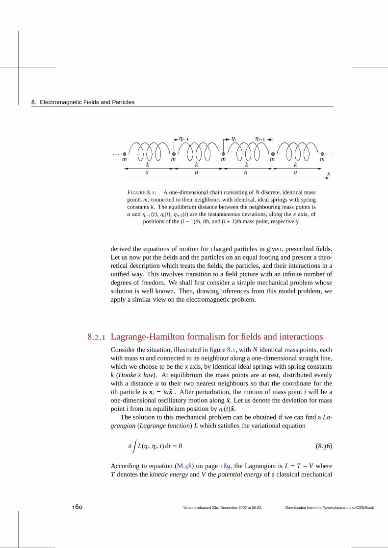
8. Electromagnetic Fields and Particles
a
ηi−1 ηi ηi+1
k k kkm m m m
x
m
a a a
FIGURE8.1: A one-dimensional chain consisting ofN discrete, identical masspointsm, connected to their neighbours with identical, ideal springs with springconstantsk. The equilibrium distance between the neighbouring mass points isa andηi−1(t), ηi(t), ηi+1(t) are the instantaneous deviations, along thex axis, of
positions of the (i − 1)th, ith, and (i + 1)th mass point, respectively.
derived the equations of motion for charged particles in given, prescribed fields.Let us now put the fields and the particles on an equal footing and present a theo-retical description which treats the fields, the particles,and their interactions in aunified way. This involves transition to a field picture with an infinite number ofdegrees of freedom. We shall first consider a simple mechanical problem whosesolution is well known. Then, drawing inferences from this model problem, weapply a similar view on the electromagnetic problem.
8.2.1 Lagrange-Hamilton formalism for fields and interactionsConsider the situation, illustrated in figure8.1, with N identical mass points, eachwith massmand connected to its neighbour along a one-dimensional straight line,which we choose to be thex axis, by identical ideal springs with spring constantsk (Hooke’s law). At equilibrium the mass points are at rest, distributed evenlywith a distancea to their two nearest neighbours so that the coordinate for theith particle isxi = iax . After perturbation, the motion of mass pointi will be aone-dimensional oscillatory motion alongx. Let us denote the deviation for masspoint i from its equilibrium position byηi(t)x.
The solution to this mechanical problem can be obtained if wecan find aLa-grangian(Lagrange function) L which satisfies the variational equation
δ
∫
L(ηi , ηi , t) dt = 0 (8.36)
According to equation (M.48) on page189, the Lagrangian isL = T − V whereT denotes thekinetic energyandV thepotential energyof a classical mechanical
160 Version released 23rd December 2007 at 00:02. Downloaded from http://www.plasma.uu.se/CED/Book
Covariant field theory
system withconservative forces. In our case the Lagrangian is
L =12
N
∑i=1
[mη2
i − k(ηi+1 − ηi)2]
(8.37)
Let us write the Lagrangian, as given by equation (8.37) above, in the follow-ing way:
L =N
∑i=1
aLi (8.38)
Here,
Li =12
[maη2
i − ka(ηi+1 − ηi
a
)2]
(8.39)
is the so called linearLagrange density. If we now let N → ∞ and, at thesame time, let the springs become infinitesimally short according to the followingscheme:
a→ dx (8.40a)
ma→ dm
dx= µ linear mass density (8.40b)
ka→ Y Young’s modulus (8.40c)
ηi+1 − ηi
a→ ∂η
∂x(8.40d)
we obtain
L =∫
L dx (8.41)
where
L
(
η,∂η
∂t,∂η
∂x, t
)
=12
[
µ
(∂η
∂t
)2
− Y
(∂η
∂x
)2]
(8.42)
Notice how we made a transition from a discrete description,in which the masspoints were identified by a discrete integer variablei = 1, 2, . . . ,N, to a continu-ous description, where the infinitesimal mass points were instead identified by acontinuous real parameterx, namely their position alongx.
A consequence of this transition is that the number of degrees of freedom forthe system went from the finite numberN to infinity! Another consequence isthatL has now become dependent also on the partial derivative withrespect to
Downloaded from http://www.plasma.uu.se/CED/Book Version released 23rd December 2007 at 00:02. 161
8. Electromagnetic Fields and Particles
x of the ‘field coordinate’η. But, as we shall see, the transition is well worth thecost because it allows us to treat all fields, be it classical scalar or vectorial fields,or wave functions, spinors and other fields that appear in quantum physics, on anequal footing.
Under the assumption of time independence and fixed endpoints, the variationprinciple (8.36) on page160 yields:
δ
∫
L dt
= δ
∫∫
L
(
η,∂η
∂t,∂η
∂x
)
dxdt
=
∫∫
∂L
∂ηδη +
∂L
∂(∂η
∂t
) δ
(∂η
∂t
)
+∂L
∂(∂η
∂x
) δ
(∂η
∂x
)
dxdt
= 0
(8.43)
The last integral can be integrated by parts. This results inthe expression
∫∫
∂L
∂η− ∂
∂t
∂L
∂(∂η
∂t
)
− ∂
∂x
∂L
∂(∂η
∂x
)
δηdxdt = 0 (8.44)
where the variation is arbitrary (and the endpoints fixed). This means that theintegrand itself must vanish. If we introduce thefunctional derivative
δL
δη=∂L
∂η− ∂
∂x
∂L
∂(∂η
∂x
)
(8.45)
we can express this as
δL
δη− ∂
∂t
∂L
∂(∂η
∂t
)
= 0 (8.46)
which is the one-dimensionalEuler-Lagrange equation.Inserting the linear mass point chain Lagrangian density, equation (8.42) on
page161, into equation (8.46), we obtain the equation of motion for our one-dimensional linear mechanical structure. It is:
µ∂2η
∂t2− Y
∂2η
∂x2=
(µ
Y∂2
∂t2− ∂2
∂x2
)
η = 0 (8.47)
i.e., the one-dimensional wave equation for compression waves which propagatewith phase speedvφ =
√Y/µ along the linear structure.
162 Version released 23rd December 2007 at 00:02. Downloaded from http://www.plasma.uu.se/CED/Book
Covariant field theory
A generalisation of the above 1D results to a three-dimensional continuum isstraightforward. For this 3D case we get the variational principle
δ
∫
L dt = δ∫∫
L d3x dt
= δ
∫
L
(
η,∂η
∂xµ
)
d4x
=
∫∫
∂L
∂η− ∂
∂xµ
∂L
∂(
∂η
∂xµ
)
δηd4x
= 0
(8.48)
where the variationδη is arbitrary and the endpoints are fixed. This means thatthe integrand itself must vanish:
∂L
∂η− ∂
∂xµ
∂L
∂(
∂η
∂xµ
)
= 0 (8.49)
This constitutes the four-dimensionalEuler-Lagrange equations.Introducing thethree-dimensional functional derivative
δL
δη=∂L
∂η− ∂
∂xi
∂L
∂(∂η
∂xi
)
(8.50)
we can express this as
δL
δη− ∂
∂t
∂L
∂(∂η
∂t
)
= 0 (8.51)
In analogy with particle mechanics (finite number of degreesof freedom), wemay introduce thecanonically conjugate momentum density
π(xµ) = π(t, x) =∂L
∂(∂η
∂t
) (8.52)
and define theHamilton density
H
(
π, η,∂η
∂xi; t
)
= π∂η
∂t−L
(
η,∂η
∂t,∂η
∂xi
)
(8.53)
Downloaded from http://www.plasma.uu.se/CED/Book Version released 23rd December 2007 at 00:02. 163
8. Electromagnetic Fields and Particles
If, as usual, we differentiate this expression and identify terms, we obtain thefollowing Hamilton density equations
∂H
∂π=∂η
∂t(8.54a)
δH
δη= −∂π
∂t(8.54b)
The Hamilton density functions are in many ways similar to the ordinary Hamiltonfunctions and lead to similar results.
The electromagnetic field
Above, when we described the mechanical field, we used a scalar field η(t, x).If we want to describe the electromagnetic field in terms of a Lagrange densityL and Euler-Lagrange equations, it comes natural to expressL in terms of thefour-potentialAµ(xκ).
The entire system of particles and fields consists of a mechanical part, a fieldpart and an interaction part. We therefore assume that the total Lagrange densityL tot for this system can be expressed as
Ltot = L
mech+Linter +L
field (8.55)
where the mechanical part has to do with the particle motion (kinetic energy). Itis given byL4/V whereL4 is given by equation (8.3) on page154 andV is thevolume. Expressed in therest mass density0, themechanical Lagrange densitycan be written
Lmech=
120u
µuµ (8.56)
The L inter part describes the interaction between the charged particles andthe external electromagnetic field. A convenient expression for this interactionLagrange densityis
Linter = jµAµ (8.57)
For the field partL field we choose the difference between magnetic and elec-tric energy density (in analogy with the difference between kinetic and potentialenergy in a mechanical field). Using the field tensor, we express thisfield La-grange densityas
Lfield =
14µ0
FµνFµν (8.58)
164 Version released 23rd December 2007 at 00:02. Downloaded from http://www.plasma.uu.se/CED/Book
Covariant field theory
so that the total Lagrangian density can be written
Ltot =
120u
µuµ + jµAµ +1
4µ0FµνFµν (8.59)
From this we can calculate all physical quantities.UsingL tot in the 3D Euler-Lagrange equations, equation (8.49) on page163
(with η replaced byAν), we can derive the dynamics for the whole system. Forinstance, the electromagnetic part of the Lagrangian density
LEM = L
inter +Lfield = jνAν +
14µ0
FµνFµν (8.60)
inserted into the Euler-Lagrange equations, expression (8.49) on page163, yieldstwo of Maxwell’s equations. To see this, we note from equation(8.60) and theresults in Example8.1 that
∂L EM
∂Aν
= jν (8.61)
Furthermore,
∂µ
[∂L EM
∂(∂µAν)
]
=1
4µ0∂µ
[∂
∂(∂µAν)
(FκλFκλ
)]
=1
4µ0∂µ
∂
∂(∂µAν)
[(∂κAλ − ∂λAκ)(∂κAλ − ∂λAκ)
]
=1
4µ0∂µ
∂
∂(∂µAν)
[
∂κAλ∂κAλ − ∂κAλ∂λAκ
− ∂λAκ∂κAλ + ∂λAκ∂λAκ
]
=1
2µ0∂µ
[∂
∂(∂µAν)
(∂κAλ∂κAλ − ∂κAλ∂λAκ
)]
(8.62)
But∂
∂(∂µAν)
(∂κAλ∂κAλ
)= ∂κAλ ∂
∂(∂µAν)∂κAλ + ∂κAλ
∂
∂(∂µAν)∂κAλ
= ∂κAλ ∂
∂(∂µAν)∂κAλ + ∂κAλ
∂
∂(∂µAν)gκα∂αg
λβAβ
= ∂κAλ ∂
∂(∂µAν)∂κAλ + g
καgλβ∂κAλ
∂
∂(∂µAν)∂αAβ
= ∂κAλ ∂
∂(∂µAν)∂κAλ + ∂
αAβ ∂
∂(∂µAν)∂αAβ
= 2∂µAν
(8.63)
Downloaded from http://www.plasma.uu.se/CED/Book Version released 23rd December 2007 at 00:02. 165
8. Electromagnetic Fields and Particles
Similarly,
∂
∂(∂µAν)
(∂κAλ∂λAκ
)= 2∂νAµ (8.64)
so that
∂µ
[∂L EM
∂(∂µAν)
]
=1µ0∂µ (∂µAν − ∂νAµ) =
1µ0∂µF
µν (8.65)
This means that the Euler-Lagrange equations, expression (8.49) on page163,for the Lagrangian densityL EM and withAν as the field quantity become
∂L EM
∂Aν
− ∂µ[∂L EM
∂(∂µAν)
]
= jν − 1µ0∂µF
µν = 0 (8.66)
or
∂µFµν = µ0 jν (8.67)
which, according to equation (7.82) on page148, is the covariant formulation ofMaxwell’s source equations.
Other fields
In general, the dynamic equations for most any fields, and notonly electromag-netic ones, can be derived from a Lagrangian density together with a variationalprinciple (the Euler-Lagrange equations). Both linear andnon-linear fields arestudied with this technique. As a simple example, consider areal, scalar fieldηwhich has the following Lagrange density:
L =12
(∂µη∂
µη −m2η2)
(8.68)
Insertion into the 1D Euler-Lagrange equation, equation (8.46) on page162, yieldsthe dynamic equation
(2 −m2)η = 0 (8.69)
with the solution
η = ei(k·x−ωt) e−m|x|
|x| (8.70)
which describes theYukawa meson fieldfor a scalar meson with massm. With
π =1c2
∂η
∂t(8.71)
166 Version released 23rd December 2007 at 00:02. Downloaded from http://www.plasma.uu.se/CED/Book
Bibliography
we obtain the Hamilton density
H =12
[c2π2 + (∇η)2 +m2η2
](8.72)
which is positive definite.Another Lagrangian density which has attracted quite some interest is the
Proca Lagrangian
LEM = L
inter +Lfield = jνAν +
14µ0
FµνFµν +m2AµAµ (8.73)
which leads to the dynamic equation
∂µFµν −m2Aν = µ0 jν (8.74)
This equation describes an electromagnetic field with a mass, or, in other words,massive photons. If massive photons would exist, large-scale magnetic fields,including those of the earth and galactic spiral arms, wouldbe significantly mod-ified to yield measurable discrepancies from their usual form. Space experimentsof this kind on board satellites have led to stringent upper bounds on the photonmass. If the photon really has a mass, it will have an impact onelectrodynamicsas well as on cosmology and astrophysics.
8.3 Bibliography[1] A. O. BARUT, Electrodynamics and Classical Theory of Fields and Particles, Dover Pub-
lications, Inc., New York, NY, 1980, ISBN 0-486-64038-8.
[2] V. L. GINZBURG, Applications of Electrodynamics in Theoretical Physics and Astro-physics, Revised third ed., Gordon and Breach Science Publishers, New York, London,Paris, Montreux, Tokyo and Melbourne, 1989, ISBN 2-88124-719-9.
[3] H. GOLDSTEIN, Classical Mechanics, second ed., Addison-Wesley Publishing Com-pany, Inc., Reading, MA . . . , 1981, ISBN 0-201-02918-9.
[4] W. T. GRANDY, Introduction to Electrodynamics and Radiation, Academic Press,New York and London, 1970, ISBN 0-12-295250-2.
[5] L. D. LANDAU AND E. M. LIFSHITZ, The Classical Theory of Fields, fourth revised En-glish ed., vol. 2 ofCourse of Theoretical Physics, Pergamon Press, Ltd., Oxford . . . , 1975,ISBN 0-08-025072-6.
[6] W. K. H. PANOFSKY AND M. PHILLIPS, Classical Electricity and Magnetism, second ed.,Addison-Wesley Publishing Company, Inc., Reading, MA . . . ,1962, ISBN 0-201-05702-6.
Downloaded from http://www.plasma.uu.se/CED/Book Version released 23rd December 2007 at 00:02. 167
8. Electromagnetic Fields and Particles
[7] J. J. SAKURAI , Advanced Quantum Mechanics, Addison-Wesley Publishing Com-pany, Inc., Reading, MA . . . , 1967, ISBN 0-201-06710-2.
[8] D. E. SOPER, Classical Field Theory, John Wiley & Sons, Inc., New York, London, Sydneyand Toronto, 1976, ISBN 0-471-81368-0.
168 Version released 23rd December 2007 at 00:02. Downloaded from http://www.plasma.uu.se/CED/Book
Example
8.4 Example
⊲FIELD ENERGY DIFFERENCE EXPRESSED IN THE FIELD TENSOR EXAMPLE 8.1
Show, by explicit calculation, that
14µ0
FµνFµν =12
(B2
µ0− ε0E2
)
(8.75)
i.e., the difference between the magnetic and electric field energy densities.
From formula (7.79) on page147 we recall that
(Fµν) =
0 −Ex/c −Ey/c −Ez/cEx/c 0 −Bz By
Ey/c Bz 0 −Bx
Ez/c −By Bx 0
(8.76)
and from formula (7.81) on page148 that
(Fµν
)=
0 Ex/c Ey/c Ez/c−Ex/c 0 −Bz By
−Ey/c Bz 0 −Bx
−Ez/c −By Bx 0
(8.77)
whereµ denotes the row number andν the column number. Then, Einstein summation anddirect substitution yields
FµνFµν = F00F00 + F01F01 + F02F02 + F03F03
+ F10F10 + F11F11 + F12F12 + F13F13
+ F20F20 + F21F21 + F22F22 + F23F23
+ F30F30 + F31F31 + F32F32 + F33F33
= 0− E2x/c
2 − E2y/c
2 − E2z/c
2
− E2x/c
2 + 0+ B2z + B2
y
− E2y/c
2 + B2z + 0+ B2
x
− E2z/c
2 + B2y + B2
x + 0
= −2E2x/c
2 − 2E2y/c
2 − 2E2z/c
2 + 2B2x + 2B2
y + 2B2z
= −2E2/c2 + 2B2 = 2(B2 − E2/c2)
(8.78)
or
14µ0
FµνFµν =12
(B2
µ0− 1
c2µ0E2
)
=12
(B2
µ0− ε0E2
)
(8.79)
where, in the last step, the identityε0µ0 = 1/c2 was used. QED
⊳ END OF EXAMPLE 8.1
Downloaded from http://www.plasma.uu.se/CED/Book Version released 23rd December 2007 at 00:02. 169

Downloaded from http://www.plasma.uu.se/CED/Book Version released 23rd December 2007 at 00:02.
FFORMULÆ
F.1 The electromagnetic field
F.1.1 Maxwell’s equations
∇ · D = ρ (F.1)
∇ · B = 0 (F.2)
∇ × E = − ∂∂t
B (F.3)
∇ × H = j +∂
∂tD (F.4)
Constitutive relations
D = εE (F.5)
H =Bµ
(F.6)
j = σE (F.7)
P = ε0χE (F.8)
171
F. Formulæ
F.1.2 Fields and potentials
Vector and scalar potentials
B = ∇ × A (F.9)
E = −∇φ − ∂
∂tA (F.10)
The Lorenz-Lorentz gauge condition in vacuum
∇ · A + 1c2
∂
∂tφ = 0 (F.11)
F.1.3 Force and energy
Poynting’s vector
S= E × H (F.12)
Maxwell’s stress tensor
Ti j = EiD j + Hi Bj −12δi j (EkDk + HkBk) (F.13)
F.2 Electromagnetic radiation
F.2.1 Relationship between the field vectors in a plane wave
B =k × E
c(F.14)
F.2.2 The far fields from an extended source distribution
Bradω (x) =
−iµ0
4πeik|x|
|x|
∫
V′d3x′ e−ik·x′ jω × k (F.15)
Eradω (x) =
i4πε0c
eik|x|
|x| x ×∫
V′d3x′ e−ik·x′ jω × k (F.16)
172 Version released 23rd December 2007 at 00:02. Downloaded from http://www.plasma.uu.se/CED/Book
Electromagnetic radiation
F.2.3 The far fields from an electric dipole
Bradω (x) = −ωµ0
4πeik|x|
|x| pω × k (F.17)
Eradω (x) = − 1
4πε0
eik|x|
|x| (pω × k) × k (F.18)
F.2.4 The far fields from a magnetic dipole
Bradω (x) = − µ0
4πeik|x|
|x|(mω × k) × k (F.19)
Eradω (x) =
k4πε0c
eik|x|
|x| mω × k (F.20)
F.2.5 The far fields from an electric quadrupole
Bradω (x) =
iµ0ω
8πeik|x|
|x| (k ·Qω) × k (F.21)
Eradω (x) =
i8πε0
eik|x|
|x| [(k ·Qω) × k] × k (F.22)
F.2.6 The fields from a point charge in arbitrary motion
E(t, x) =q
4πε0s3
[
(x − x0)
(
1− v′2
c2
)
+ (x − x′) ×(x − x0) × v′
c2
]
(F.23)
B(t, x) = (x − x′) ×E(t, x)
c|x − x′| (F.24)
s=∣∣x − x′
∣∣ − (x − x′) · v
′
c(F.25)
x − x0 = (x − x′) − |x − x′|v′
c(F.26)
(∂t′
∂t
)
x=|x − x′|
s(F.27)
Downloaded from http://www.plasma.uu.se/CED/Book Version released 23rd December 2007 at 00:02. 173
F. Formulæ
F.3 Special relativity
F.3.1 Metric tensor
gµν =
1 0 0 00 −1 0 00 0 −1 00 0 0 −1
(F.28)
F.3.2 Covariant and contravariant four-vectors
vµ = gµνvν (F.29)
F.3.3 Lorentz transformation of a four-vector
x′µ = Λµνxν (F.30)
Λµν =
γ −γβ 0 0−γβ γ 0 0
0 0 1 00 0 0 1
(F.31)
γ =1
√
1− β2(F.32)
β =v
c(F.33)
F.3.4 Invariant line element
ds= cdtγ= cdτ (F.34)
F.3.5 Four-velocity
uµ =dxdτ
µ
= γ(c, v) (F.35)
174 Version released 23rd December 2007 at 00:02. Downloaded from http://www.plasma.uu.se/CED/Book
Vector relations
F.3.6 Four-momentum
pµ = m0uµ =
(Ec, p)
(F.36)
F.3.7 Four-current densityjµ = ρ0u
µ (F.37)
F.3.8 Four-potential
Aµ =
(φ
c, A)
(F.38)
F.3.9 Field tensor
Fµν = ∂µAν − ∂νAµ =
0 −Ex/c −Ey/c −Ez/cEx/c 0 −Bz ByEy/c Bz 0 −Bx
Ez/c −By Bx 0
(F.39)
F.4 Vector relationsLet x be the radius vector (coordinate vector) from the origin to the point(x1, x2, x3) ≡ (x, y, z) and let |x| denote the magnitude (‘length’) ofx. Let fur-therα(x), β(x), . . . be arbitrary scalar fields anda(x), b(x), c(x), d(x), . . . arbitraryvector fields.
The differential vector operator∇ is in Cartesian coordinates given by
∇ ≡3
∑i=1
xi∂
∂xi
def≡ xi∂
∂xi
def≡ ∂ (F.40)
where xi , i = 1, 2, 3 is theith unit vector andx1 ≡ x, x2 ≡ y, and x3 ≡ z. Incomponent (tensor) notation∇ can be written
∇i = ∂i =
(∂
∂x1,∂
∂x2,∂
∂x3
)
=
(∂
∂x,∂
∂y,∂
∂z
)
(F.41)
Downloaded from http://www.plasma.uu.se/CED/Book Version released 23rd December 2007 at 00:02. 175

F. Formulæ
F.4.1 Spherical polar coordinates
Base vectors
r = sinθ cosϕx1 + sinθ sinϕx2 + cosθx3 (F.42a)
θ = cosθ cosϕx1 + cosθ sinϕx2 − sinθx3 (F.42b)
ϕ = − sinϕx1 + cosϕx2 (F.42c)
x1 = sinθ cosϕr + cosθ cosϕθ − sinϕϕ (F.43a)
x2 = sinθ sinϕr + cosθ sinϕθ + cosϕϕ (F.43b)
x3 = cosθ r − sinθθ (F.43c)
Directed line element
dx x = dl = dr r + r dθ θ + r sinθ dϕ ϕ (F.44)
Solid angle element
dΩ = sinθ dθ dϕ (F.45)
Directed area element
d2x n = dS= dS r = r2dΩ r (F.46)
Volume element
d3x = dV = dr dS = r2dr dΩ (F.47)
F.4.2 Vector formulae
General vector algebraic identities
a · b = b · a = δi j aibj = abcosθ (F.48)
a× b = −b × a = ǫi jkajbkxi (F.49)
a · (b × c) = (a× b) · c (F.50)
a× (b × c) = b(a · c) − c(a · b) ≡ ba · c− ca · b (F.51)
a× (b × c) + b × (c× a) + c× (a× b) = 0 (F.52)
176 Version released 23rd December 2007 at 00:02. Downloaded from http://www.plasma.uu.se/CED/Book
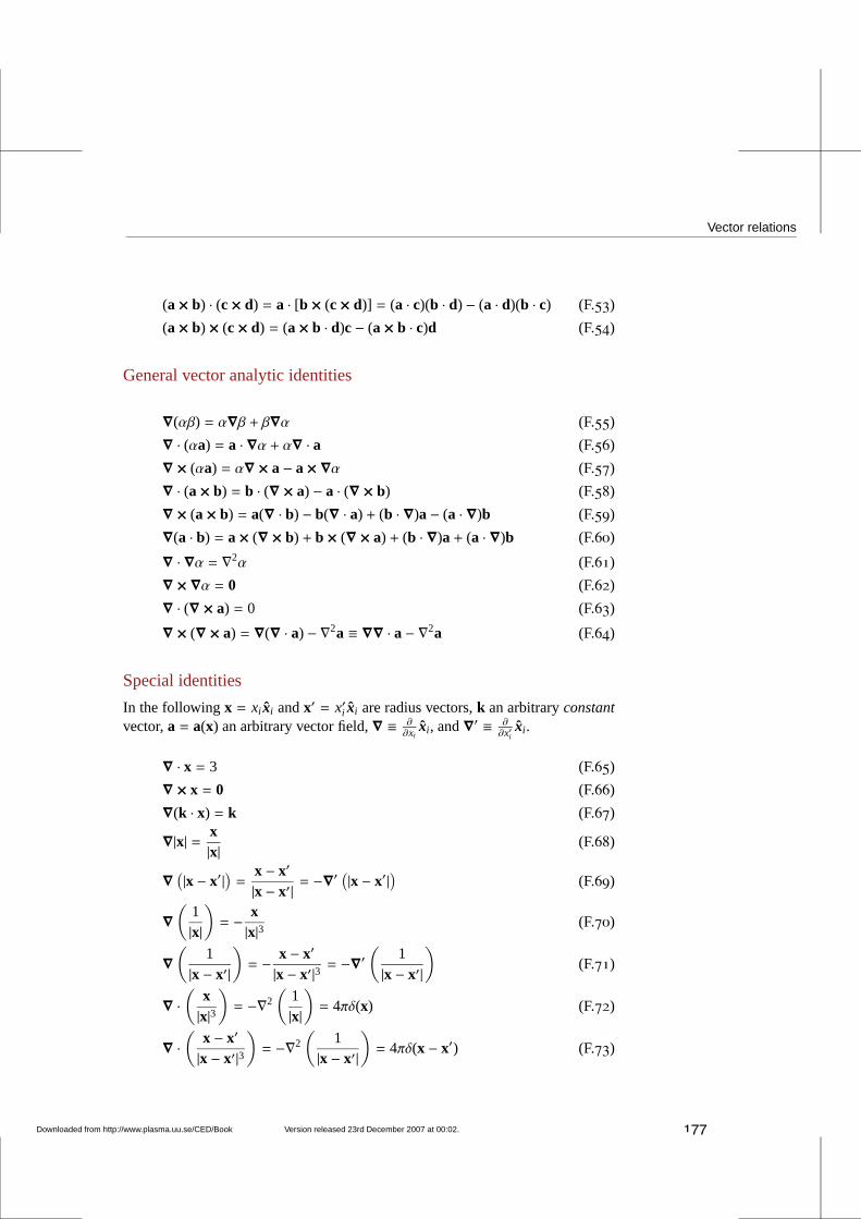
Vector relations
(a× b) · (c× d) = a · [b × (c× d)] = (a · c)(b · d) − (a · d)(b · c) (F.53)
(a× b) × (c× d) = (a× b · d)c− (a× b · c)d (F.54)
General vector analytic identities
∇(αβ) = α∇β + β∇α (F.55)
∇ · (αa) = a · ∇α + α∇ · a (F.56)
∇ × (αa) = α∇ × a− a× ∇α (F.57)
∇ · (a× b) = b · (∇ × a) − a · (∇ × b) (F.58)
∇ × (a× b) = a(∇ · b) − b(∇ · a) + (b · ∇)a− (a · ∇)b (F.59)
∇(a · b) = a× (∇ × b) + b × (∇ × a) + (b · ∇)a+ (a · ∇)b (F.60)
∇ · ∇α = ∇2α (F.61)
∇ × ∇α = 0 (F.62)
∇ · (∇ × a) = 0 (F.63)
∇ × (∇ × a) = ∇(∇ · a) − ∇2a ≡ ∇∇ · a− ∇2a (F.64)
Special identities
In the followingx = xi xi andx′ = x′i xi are radius vectors,k an arbitraryconstantvector,a = a(x) an arbitrary vector field,∇ ≡ ∂
∂xixi , and∇′ ≡ ∂
∂x′ixi .
∇ · x = 3 (F.65)
∇ × x = 0 (F.66)
∇(k · x) = k (F.67)
∇|x| = x|x| (F.68)
∇(|x − x′|
)=
x − x′
|x − x′| = −∇′ (|x − x′|
)(F.69)
∇
(1|x|
)
= − x|x|3 (F.70)
∇
(1
|x − x′|
)
= − x − x′
|x − x′|3 = −∇′(
1|x − x′|
)
(F.71)
∇ ·(
x|x|3
)
= −∇2
(1|x|
)
= 4πδ(x) (F.72)
∇ ·(
x − x′
|x − x′|3
)
= −∇2
(1
|x − x′|
)
= 4πδ(x − x′) (F.73)
Downloaded from http://www.plasma.uu.se/CED/Book Version released 23rd December 2007 at 00:02. 177
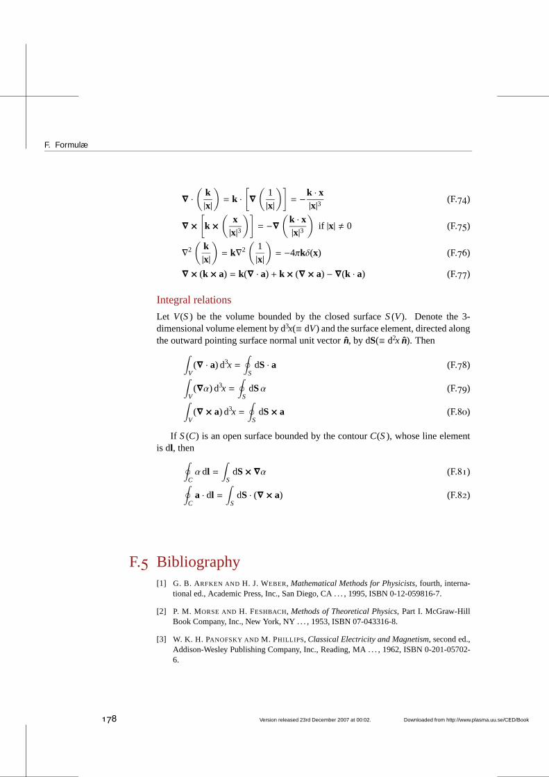
F. Formulæ
∇ ·(
k|x|
)
= k ·[
∇
(1|x|
)]
= −k · x|x|3 (F.74)
∇ ×
[
k ×(
x|x|3
)]
= −∇(
k · x|x|3
)
if |x| , 0 (F.75)
∇2
(k|x|
)
= k∇2
(1|x|
)
= −4πkδ(x) (F.76)
∇ × (k × a) = k(∇ · a) + k × (∇ × a) − ∇(k · a) (F.77)
Integral relations
Let V(S) be the volume bounded by the closed surfaceS(V). Denote the 3-dimensional volume element by d3x(≡ dV) and the surface element, directed alongthe outward pointing surface normal unit vectorn, by dS(≡ d2x n). Then
∫
V(∇ · a) d3x =
∮
SdS · a (F.78)
∫
V(∇α) d3x =
∮
SdSα (F.79)
∫
V(∇ × a) d3x =
∮
SdS× a (F.80)
If S(C) is an open surface bounded by the contourC(S), whose line elementis dl, then
∮
Cαdl =
∫
SdS× ∇α (F.81)
∮
Ca · dl =
∫
SdS · (∇ × a) (F.82)
F.5 Bibliography[1] G. B. ARFKEN AND H. J. WEBER, Mathematical Methods for Physicists, fourth, interna-
tional ed., Academic Press, Inc., San Diego, CA . . . , 1995, ISBN 0-12-059816-7.
[2] P. M. MORSE AND H. FESHBACH, Methods of Theoretical Physics, Part I. McGraw-HillBook Company, Inc., New York, NY . . . , 1953, ISBN 07-043316-8.
[3] W. K. H. PANOFSKY AND M. PHILLIPS, Classical Electricity and Magnetism, second ed.,Addison-Wesley Publishing Company, Inc., Reading, MA . . . ,1962, ISBN 0-201-05702-6.
178 Version released 23rd December 2007 at 00:02. Downloaded from http://www.plasma.uu.se/CED/Book
Downloaded from http://www.plasma.uu.se/CED/Book Version released 23rd December 2007 at 00:02.
MMATHEMATICAL METHODS
M.1 Scalars, vectors and tensors
Every physical observable can be described by a geometric object. We have cho-sen to describe the observables in classical electrodynamics in terms of scalars,pseudoscalars, vectors, pseudovectors, tensors or pseudotensors, all of which obeycertain canonical rules of transformation under a change ofcoordinate systems.We will not exploit differential forms to any significant degree to describe physicalobservables.
A scalardescribes a scalar quantity which may or may not be constant in timeand/or space. Avector describes some kind of physical motion along a curvein space due to vection and atensordescribes the local motion or deformationof a surface or a volume due to some form of tension. However, generalisationsto more abstract notions of these quantities have proved useful and are thereforecommonplace. The difference between a scalar, vector and tensor and apseu-doscalar, pseudovectorand apseudotensoris that the latter behave differentlyunder such coordinate transformations which cannot be reduced to pure rotations.
Throughout we adopt the convention that Latin indicesi, j, k, l, . . . run overthe range 1, 2, 3 to denote vector or tensor components in the real Euclideanthree-dimensional (3D) configuration spaceR3, and Greek indicesµ, ν, κ, λ, . . . , whichare used in four-dimensional (4D) space, run over the range 0, 1, 2, 3.
179
M. Mathematical Methods
M.1.1 Vectors
Radius vector
Mathematically, a vector can be represented in a number of different ways. Onesuitable representation in a real or complex1 vector space of dimensionalityNis in terms of an orderedN-tuple of real or complex numbers, or arow vectorof the components, (a1, a2, . . . , aN), along theN coordinate axes that span thevector space under consideration. Note, however, that there are many orderedN-tuples of numbers that do not comprise a vector,i.e., do not exhibit vectortransformation properties! The most basic vector, and the prototype against whichall other vectors are benchmarked, is theradius vectorwhich is the vector fromthe origin to the point of interest. ItsN-tuple representation simply enumeratesthe coordinates which describe this point. In this sense, the radius vector from theorigin to a point is synonymous with the coordinates of the point itself.
In the 3D Euclidean spaceR3, we haveN = 3 and the radius vector can berepresented by the triplet (x1, x2, x3) of coordinatesxi , i = 1, 2, 3. The coordinatesxi are scalar quantities which describe the position along theunit base vectorsxi
which spanR3. Therefore a representation of the radius vector inR3 is
x =3
∑i=1
xi xidef≡ xi xi (M.1)
where we have introducedEinstein’s summation convention(EΣ) which statesthat a repeated index in a term implies summation over the range of the indexin question. Whenever possible and convenient we shall in the following alwaysassume EΣ and suppress explicit summation in our formulae. Typographically,we represent a vector in 3D Euclidean spaceR3 by a boldface letter or symbolin a Roman font. Moreover, we introduced the symbol≡def which may be read‘is, by definition, to equal in meaning’, or ‘equals by definition’, or, formally,definiendum≡def definiens[4].
Alternatively, we may describe the radius vector incomponent notationasfollows:
xidef≡ (x1, x2, x3) ≡ (x, y, z) (M.2)
This component notation is particularly useful in 4D space where we can rep-
1It is often very convenient to usecomplex notationin physics. This notation can simplify the mathe-matical treatment considerably. But since all physical observables are real, we must in the final step of ourmathematical analysis of a physical problem always ensure that the results to be compared with experimen-tal values are real-valued. In classical physics this is achieved by taking the real (or imaginary) part of themathematical result, whereas in quantum physics one takes the absolute value.
180 Version released 23rd December 2007 at 00:02. Downloaded from http://www.plasma.uu.se/CED/Book
Scalars, vectors and tensors
resent the radius vector either in itscontravariant component form
xµdef≡ (x0, x1, x2, x3) (M.3)
or its covariant component form
xµdef≡ (x0, x1, x2, x3) (M.4)
The relation between the covariant and contravariant formsis determined by themetric tensor(also known as thefundamental tensor) whose actual form is dic-tated by the properties of the vector space in question. The dual representationof vectors in contravariant and covariant forms is most convenient when we workin a non-Euclidean vector space with an indefinitemetric. An example isLorentzspaceL4 which is a 4DRiemannian spaceutilised to formulate the special theoryof relativity.
We note that for a change of coordinatesxµ → x′µ = x′µ(x0, x1, x2, x3), dueto a transformation from a systemΣ to another systemΣ′, the differential radiusvector dxµ transforms as
dx′µ =∂x′µ
∂xνdxν (M.5)
which follows trivially from the rules of differentiation ofx′µ considered as func-tions of four variablesxν.
M.1.2 FieldsA field is a physical entity which depends on one or more continuous parameters.Such a parameter can be viewed as a ‘continuous index’ which enumerates the‘coordinates’ of the field. In particular, in a field which depends on the usualradius vectorx of R3, each point in this space can be considered as one degree offreedom so that a field is a representation of a physical entity which has an infinitenumber of degrees of freedom.
Scalar fields
We denote an arbitraryscalar fieldin R3 by
α(x) = α(x1, x2, x3)def≡ α(xi) (M.6)
This field describes how the scalar quantityα varies continuously in 3DR3 space.In 4D, afour-scalarfield is denoted
α(x0, x1, x2, x3)def≡ α(xµ) (M.7)
Downloaded from http://www.plasma.uu.se/CED/Book Version released 23rd December 2007 at 00:02. 181
M. Mathematical Methods
which indicates that the four-scalarα depends on all four coordinates spanningthis space. Since a four-scalar has the same value at a given point regardless ofcoordinate system, it is also called aninvariant.
Analogous to the transformation rule, equation (M.5) on page181, for thedifferential dxµ, the transformation rule for the differential operator∂/∂xµ under atransformationxµ → x′µ becomes
∂
∂x′µ=∂xν
∂x′µ∂
∂xν(M.8)
which, again, follows trivially from the rules of differentiation.
Vector fields
We can represent an arbitrary vector fielda(x) in R3 as follows:
a(x) = ai(x)xi (M.9)
In component notation this same vector can be represented as
ai(x) = (a1(x), a2(x), a3(x)) = ai(xj) (M.10)
In 4D, an arbitraryfour-vectorfield in contravariant component form can berepresented as
aµ(xν) = (a0(xν), a1(xν), a2(xν), a3(xν)) (M.11)
or, in covariantcomponent form, as
aµ(xν) = (a0(x
ν), a1(xν), a2(x
ν), a3(xν)) (M.12)
wherexν is the radius four-vector. Again, the relation betweenaµ andaµ is deter-mined by the metric of the physical 4D system under consideration.
Whether an arbitraryN-tuple fulfils the requirement of being an (N-dimen-sional) contravariant vector or not, depends on its transformation properties duringa change of coordinates. For instance, in 4D an assemblageyµ = (y0, y1, y2, y3)constitutes acontravariant four-vector(or the contravariant components of a four-vector) if and only if, during a transformation from a systemΣ with coordinatesxµ to a systemΣ′ with coordinatesx′µ, it transforms to the new system accordingto the rule
y′µ =∂x′µ
∂xνyν (M.13)
i.e., in the same way as the differential coordinate element dxµ transforms accord-ing to equation (M.5) on page181.
182 Version released 23rd December 2007 at 00:02. Downloaded from http://www.plasma.uu.se/CED/Book
Scalars, vectors and tensors
The analogous requirement for acovariant four-vectoris that it transforms,during the change fromΣ to Σ′, according to the rule
y′µ =∂xν
∂x′µyν (M.14)
i.e., in the same way as the differential operator∂/∂xµ transforms according toequation (M.8) on page182.
Tensor fields
We denote an arbitrarytensor fieldin R3 by A(x). This tensor field can be repre-sented in a number of ways, for instance in the followingmatrix form:
(Ai j (xk)
) def≡
A11(x) A12(x) A13(x)A21(x) A22(x) A23(x)A31(x) A32(x) A33(x)
(M.15)
Strictly speaking, the tensor field described here is a tensor of rank two.A particularly simple rank-two tensor inR3 is the 3DKronecker deltasymbol
δi j , with the following properties:
δi j =
0 if i , j
1 if i = j(M.16)
The 3D Kronecker delta has the following matrix representation
(δi j ) =
1 0 00 1 00 0 1
(M.17)
Another common and useful tensor is the fully antisymmetrictensor of rank 3,also known as theLevi-Civita tensor
ǫi jk =
1 if i, j, k is anevenpermutation of 1,2,3
0 if at least two ofi, j, k are equal
−1 if i, j, k is anoddpermutation of 1,2,3
(M.18)
with the following further property
ǫi jkǫilm = δ jlδkm− δ jmδkl (M.19)
In fact, tensors may have any rankn. In this picture a scalar is considered tobe a tensor of rankn = 0 and a vector a tensor of rankn = 1. Consequently, the
Downloaded from http://www.plasma.uu.se/CED/Book Version released 23rd December 2007 at 00:02. 183
M. Mathematical Methods
notation where a vector (tensor) is represented in its component form is called thetensor notation. A tensor of rankn = 2 may be represented by a two-dimensionalarray or matrix whereas higher rank tensors are best represented in their compo-nent forms (tensor notation).
In 4D, we have three forms offour-tensor fieldsof rankn. We speak of
• acontravariant four-tensor field, denotedAµ1µ2...µn(xν),
• acovariant four-tensor field, denotedAµ1µ2...µn(xν),
• amixed four-tensor field, denotedAµ1µ2...µkµk+1...µn (xν).
The 4Dmetric tensor(fundamental tensor) mentioned above is a particularlyimportant four-tensor of rank 2. In covariant component form we shall denote itgµν. This metric tensor determines the relation between an arbitrary contravariantfour-vectoraµ and its covariant counterpartaµ according to the following rule:
aµ(xκ)
def≡ gµνaν(xκ) (M.20)
This rule is often calledlowering of index. The raising of indexanalogue of theindex lowering rule is:
aµ(xκ)def≡ gµνaν(x
κ) (M.21)
More generally, the following lowering and raising rules hold for arbitraryrankn mixed tensor fields:
gµkνkAν1ν2...νk−1νkνk+1νk+2...νn
(xκ) = Aν1ν2...νk−1µkνk+1...νn
(xκ) (M.22)
gµkνkAν1ν2...νk−1νkνk+1...νn
(xκ) = Aν1ν2...νk−1µkνk+1νk+2...νn
(xκ) (M.23)
Successive lowering and raising of more than one index is achieved by a repeatedapplication of this rule. For example, a dual application ofthe lowering operationon a rank 2 tensor in contravariant form yields
Aµν = gµκgλνAκλ (M.24)
i.e., the same rank 2 tensor in covariant form. This operation is also known as atensor contraction.
184 Version released 23rd December 2007 at 00:02. Downloaded from http://www.plasma.uu.se/CED/Book
Scalars, vectors and tensors
M.1.3 Vector algebra
Scalar product
Thescalar product(dot product, inner product) of two arbitrary 3D vectorsa andb in ordinaryR3 space is the scalar number
a · b = ai xi · bj x j = xi · x jaibj = δi j aibj = aibi (M.25)
where we used the fact that the scalar productxi · x j is a representation of theKronecker deltaδi j defined in equation (M.16) on page183. In Russian literature,the 3D scalar product is often denoted (ab). The scalar product ofa in R3 withitself is
a · a def≡ (a)2 = |a|2 = (ai)2 = a2 (M.26)
and similarly forb. This allows us to write
a · b = abcosθ (M.27)
whereθ is the angle betweena andb.In 4D space we define the scalar product of two arbitrary four-vectorsaµ and
bµ in the following way
aµbµ = gνµa
νbµ = aνbν = gµνaµbν (M.28)
where we made use of the index lowering and raising rules (M.20) and (M.21).The result is a four-scalar,i.e., an invariant which is independent of in which 4Dcoordinate system it is measured.
Thequadratic differential form
ds2 = gµνdxνdxµ = dxµdxµ (M.29)
i.e., the scalar product of the differential radius four-vector with itself, is an in-variant called themetric. It is also the square of theline elementds which is thedistance between neighbouring points with coordinatesxµ andxµ + dxµ.
Dyadic product
Thedyadic productfield A(x) ≡ a(x)b(x) with two juxtaposed vector fieldsa(x)andb(x) is theouter productof a andb. Operating on this dyad from the rightand from the left with an inner product of an vectorc one obtains
A · c def≡ ab · c def≡ a(b · c) (M.30a)
Downloaded from http://www.plasma.uu.se/CED/Book Version released 23rd December 2007 at 00:02. 185
M. Mathematical Methods
c · A def≡ c · abdef≡ (c · a)b (M.30b)
i.e., new vectors, proportional toa andb, respectively. In mathematics, a dyadicproduct is often calledtensor productand is frequently denoteda⊗ b.
In matrix notation the outer product ofa andb is written
(ab)=(
x1 x2 x3)
a1b1 a1b2 a1b3
a2b1 a2b2 a2b3
a3b1 a3b2 a3b3
x1
x2
x3
(M.31)
which means that we can represent the tensorA(x) in matrix form as
(Ai j (xk)
)=
a1b1 a1b2 a1b3
a2b1 a2b2 a2b3
a3b1 a3b2 a3b3
(M.32)
which we identify with expression (M.15) on page183, viz. a tensor in matrixnotation.
Vector product
Thevector productor cross productof two arbitrary 3D vectorsa andb in ordi-naryR3 space is the vector
c = a× b = ǫi jkajbkxi (M.33)
Hereǫi jk is the Levi-Civita tensor defined in equation (M.18) on page183. Some-times the 3D vector product ofa andb is denoteda ∧ b or, particularly in theRussian literature, [ab]. Alternatively,
a× b = absinθ e (M.34)
whereθ is the angle betweena andb and e is a unit vector perpendicular to theplane spanned bya andb.
A spatial reversal of the coordinate system (x′1, x′2, x′3) = (−x1,−x2,−x3) changes
sign of the components of the vectorsa andb so that in the new coordinate systema′ = −a andb′ = −b, which is to say that the direction of an ordinary vector is notdependent on the choice of directions of the coordinate axes. On the other hand,as is seen from equation (M.33), the cross product vectorc does not change sign.Thereforea (or b) is an example of a ‘true’ vector, orpolar vector, whereasc isan example of anaxial vector, or pseudovector.
A prototype for a pseudovector is the angular momentum vector L = x × pand hence the attribute ‘axial’. Pseudovectors transform as ordinary vectors undertranslations and proper rotations, but reverse their sign relative to ordinary vectors
186 Version released 23rd December 2007 at 00:02. Downloaded from http://www.plasma.uu.se/CED/Book
Scalars, vectors and tensors
for any coordinate change involving reflection. Tensors (ofany rank) which trans-form analogously to pseudovectors are calledpseudotensors. Scalars are tensorsof rank zero, and zero-rank pseudotensors are therefore also calledpseudoscalars,an example being the pseudoscalarxi · (x j × xk). This triple product is a repre-sentation of thei jk component of the Levi-Civita tensorǫi jk which is a rank threepseudotensor.
M.1.4 Vector analysis
Thedeloperator
In R3 thedel operatoris adifferential vector operator, denoted inGibbs’ notationby∇ and defined as
∇def≡ xi
∂
∂xi
def≡ ∂
∂xdef≡ ∂ (M.35)
where xi is the ith unit vector in a Cartesian coordinate system. Since the op-erator in itself has vectorial properties, we denote it witha boldface nab-la. In‘component’ notation we can write
∂i =
(∂
∂x1,∂
∂x2,∂
∂x3
)
(M.36)
In 4D, the contravariant component representation of thefour-del operatorisdefined by
∂µ =
(∂
∂x0,∂
∂x1,∂
∂x2,∂
∂x3
)
(M.37)
whereas the covariant four-del operator is
∂µ =
(∂
∂x0,∂
∂x1,∂
∂x2,∂
∂x3
)
(M.38)
We can use this four-del operator to express the transformation properties(M.13) and (M.14) on page183 as
y′µ =(∂νx′µ) yν (M.39)
and
y′µ =(∂′µxν
)yν (M.40)
respectively.With the help of the del operator we can define the gradient, divergence and
curl of a tensor (in the generalised sense).
Downloaded from http://www.plasma.uu.se/CED/Book Version released 23rd December 2007 at 00:02. 187
M. Mathematical Methods
The gradient
Thegradientof anR3 scalar fieldα(x), denoted∇α(x), is anR3 vector fielda(x):
∇α(x) = ∂α(x) = xi∂iα(x) = a(x) (M.41)
From this we see that the boldface notation for the nabla and del operators is veryhandy as it elucidates the 3D vectorial property of the gradient.
In 4D, thefour-gradientis a covariant vector, formed as a derivative of a four-scalar fieldα(xµ), with the following component form:
∂µα(xν) =∂α(xν)∂xµ
(M.42)
The divergence
We define the 3Ddivergenceof a vector field inR3 as
∇ · a(x) = ∂ · x jaj(x) = δi j∂iaj(x) = ∂iai(x) =∂ai(x)∂xi
= α(x) (M.43)
which, as indicated by the notationα(x), is ascalarfield in R3. We may think ofthe divergence as a scalar product between a vectorial operator and a vector. Asis the case for any scalar product, the result of a divergenceoperation is a scalar.Again we see that the boldface notation for the 3D del operator is very convenient.
Thefour-divergenceof a four-vectoraµ is the following four-scalar:
∂µaµ(xν) = ∂µaµ(x
ν) =∂aµ(xν)∂xµ
(M.44)
The Laplacian
The 3DLaplace operatoror Laplaciancan be described as the divergence of thegradient operator:
∇2 = ∆ = ∇ · ∇ = ∂
∂xixi · x j
∂
∂xj= δi j∂i∂ j = ∂
2i =
∂2
∂x2i
≡3
∑i=1
∂2
∂x2i
(M.45)
The symbol∇2 is sometimes readdel squared. If, for a scalar fieldα(x), ∇2α < 0at some point in 3D space, it is a sign ofconcentrationof α at that point.
The curl
In R3 thecurl of a vector fielda(x), denoted∇ × a(x), is anotherR3 vector fieldb(x) which can be defined in the following way:
∇ × a(x) = ǫi jk xi∂ jak(x) = ǫi jk xi∂ak(x)∂xj
= b(x) (M.46)
188 Version released 23rd December 2007 at 00:02. Downloaded from http://www.plasma.uu.se/CED/Book
Analytical mechanics
where use was made of the Levi-Civita tensor, introduced in equation (M.18) onpage183.
The covariant 4D generalisation of the curl of a four-vectorfield aµ(xν) is theantisymmetric four-tensor field
Gµν(xκ) = ∂µaν(x
κ) − ∂νaµ(xκ) = −Gνµ(xκ) (M.47)
A vector with vanishing curl is said to beirrotational.Numerous vector algebra and vector analysis formulae are given in chapterF.
Those which are not found there can often be easily derived byusing the compo-nent forms of the vectors and tensors, together with the Kronecker and Levi-Civitatensors and their generalisations to higher ranks. A short but very useful referencein this respect is the article by A. Evett [3].
M.2 Analytical mechanics
M.2.1 Lagrange’s equationsAs is well known from elementary analytical mechanics, theLagrange functionor Lagrangian Lis given by
L(qi , qi , t) = L
(
qi ,dqi
dt, t
)
= T − V (M.48)
whereqi is thegeneralised coordinate, T the kinetic energyandV the potentialenergyof a mechanical system, Using the action
S =∫ t2
t1dt L(qi , qi , t) (M.49)
and thevariational principlewith fixed endpointst1 andt2,
δS = 0 (M.50)
one finds that the Lagrangian satisfies theEuler-Lagrange equations
ddt
(∂L∂qi
)
− ∂L∂qi= 0 (M.51)
To the generalised coordinateqi one defines acanonically conjugate momen-tum pi according to
pi =∂L∂qi
(M.52)
Downloaded from http://www.plasma.uu.se/CED/Book Version released 23rd December 2007 at 00:02. 189
M. Mathematical Methods
and note from equation (M.51) on page189 that
∂L∂qi= pi (M.53)
If we introduce an arbitrary, differentiable functionα = α(qi , t) and a newLagrangianL′ related toL in the following way
L′ = L +dαdt= L + qi
∂α
∂qi+∂α
∂t(M.54)
then
∂L′
∂qi=∂L∂qi+∂α
∂q(M.55a)
∂L′
∂qi=∂L∂qi+
ddt∂α
∂q(M.55b)
Or, in other words,
ddt
(∂L′
∂qi
)
− ∂L′
∂qi=
ddt
( ∂L∂qi
)
− ∂L∂qi
(M.56)
where
p′i =∂L′
∂qi=∂L∂qi+∂α
∂qi= pi +
∂α
∂qi(M.57a)
and
q′i = −∂L′
∂pi=∂L∂p= qi (M.57b)
M.2.2 Hamilton’s equationsFromL, theHamiltonian(Hamilton function) H can be defined via theLegendretransformation
H(pi , qi , t) = pi qi − L(qi , qi , t) (M.58)
After differentiating the left and right hand sides of this definition and setting themequal we obtain
∂H∂pi
dpi +∂H∂qi
dqi +∂H∂t
dt = qidpi + pidqi −∂L∂qi
dqi −∂L∂qi
dqi −∂L∂t
dt
(M.59)
190 Version released 23rd December 2007 at 00:02. Downloaded from http://www.plasma.uu.se/CED/Book
Analytical mechanics
According to the definition ofpi , equation (M.52) on page189, the second andfourth terms on the right hand side cancel. Furthermore, noting that accordingto equation (M.53) on page190 the third term on the right hand side of equa-tion (M.59) on page190 is equal to−pidqi and identifying terms, we obtain theHamilton equations:
∂H∂pi= qi =
dqi
dt(M.60a)
∂H∂qi= − pi = −
dpi
dt(M.60b)
Downloaded from http://www.plasma.uu.se/CED/Book Version released 23rd December 2007 at 00:02. 191
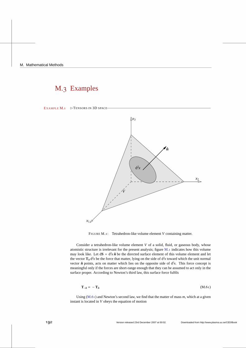
M. Mathematical Methods
M.3 Examples
⊲TENSORS IN3D SPACEEXAMPLE M.1
x1
V
d2x
n
x3
x2
FIGURE M.1: Tetrahedron-like volume elementV containing matter.
Consider a tetrahedron-like volume elementV of a solid, fluid, or gaseous body, whoseatomistic structure is irrelevant for the present analysis; figureM.1 indicates how this volumemay look like. Let dS = d2x n be the directed surface element of this volume element and letthe vectorT n d2x be the force that matter, lying on the side of d2x toward which the unit normalvector n points, acts on matter which lies on the opposite side of d2x. This force concept ismeaningful only if the forces are short-range enough that they can be assumed to act only in thesurface proper. According to Newton’s third law, this surface force fulfils
T−n = − T n (M.61)
Using (M.61) and Newton’s second law, we find that the matter of massm, which at a giveninstant is located inV obeys the equation of motion
192 Version released 23rd December 2007 at 00:02. Downloaded from http://www.plasma.uu.se/CED/Book
Examples
T n d2x− cosθ1T x1 d2x− cosθ2T x2 d2x− cosθ3T x3 d2x+ Fext = ma (M.62)
whereFext is the external force anda is the acceleration of the volume element. In other words
T n = n1T x1 + n2T x2 + n3T x3 +md2x
(
a− Fext
m
)
(M.63)
Since botha andFext/m remain finite whereasm/d2x→ 0 asV → 0, one finds that in this limit
T n =
3
∑i=1
niT xi ≡ niT xi (M.64)
From the above derivation it is clear that equation (M.64) is valid not only in equilibrium butalso when the matter inV is in motion.
Introducing the notation
Ti j =(T xi
)
j(M.65)
for the jth component of the vectorT xi , we can write equation (M.64) above in component formas follows
Tn j = (T n) j =
3
∑i=1
niTi j ≡ niTi j (M.66)
Using equation (M.66), we find that the component of the vectorT n in the direction of anarbitrary unit vectorm is
Tnm = T n · m
=
3
∑j=1
Tn jmj =
3
∑j=1
(3
∑i=1
niTi j
)
mj ≡ niTi j mj = n · T · m(M.67)
Hence, thejth component of the vectorT xi , here denotedTi j , can be interpreted as thei j thcomponent of a tensorT. Note thatTnm is independent of the particular coordinate system usedin the derivation.
We shall now show how one can use the momentum law (force equation) to derive theequation of motion for an arbitrary element of mass in the body. To this end we consider apartV of the body. If the external force density (force per unit volume) is denoted byf and thevelocity for a mass element dm is denoted byv, we obtain
ddt
∫
Vv dm=
∫
Vf d3x+
∫
ST n d2x (M.68)
The jth component of this equation can be written∫
V
ddtv j dm=
∫
Vf j d3x+
∫
STn j d2x =
∫
Vf j d3x+
∫
SniTi j d2x (M.69)
where, in the last step, equation (M.66) above was used. Setting dm = ρ d3x and using thedivergence theorem on the last term, we can rewrite the result as
∫
Vρ
ddtv j d3x =
∫
Vf j d3x+
∫
V
∂Ti j
∂xid3x (M.70)
Downloaded from http://www.plasma.uu.se/CED/Book Version released 23rd December 2007 at 00:02. 193
M. Mathematical Methods
Since this formula is valid for any arbitrary volume, we mustrequire that
ρddtv j − f j −
∂Ti j
∂xi= 0 (M.71)
or, equivalently
ρ∂v j
∂t+ ρv · ∇v j − f j −
∂Ti j
∂xi= 0 (M.72)
Note that∂v j/∂t is the rate of change with time of the velocity componentv j at afixedpointx = (x1, x1, x3).
⊳ END OF EXAMPLE M.1
⊲CONTRAVARIANT AND COVARIANT VECTORS IN FLAT LORENTZ SPACEEXAMPLE M.2
The 4D Lorentz spaceL4 has a simple metric which can be described either by the metrictensor
gµν =
1 if µ = ν = 0
−1 if µ = ν = i = j = 1,2,3
0 if µ , ν
(M.73)
which, in matrix notation, is represented as
(gµν) =
1 0 0 00 −1 0 00 0 −1 00 0 0 −1
(M.74)
i.e., a matrix with a main diagonal that has the sign sequence, orsignature, +,−,−,− or
gµν =
−1 if µ = ν = 0
1 if µ = ν = i = j = 1,2,3
0 if µ , ν
(M.75)
which, in matrix notation, is represented as
(gµν) =
−1 0 0 00 1 0 00 0 1 00 0 0 1
(M.76)
i.e., a matrix with signature−,+,+,+.
Consider an arbitrary contravariant four-vectoraν in this space. In component form it canbe written:
aνdef≡ (a0, a1,a2,a3) = (a0,a) (M.77)
194 Version released 23rd December 2007 at 00:02. Downloaded from http://www.plasma.uu.se/CED/Book
Examples
According to the index lowering rule, equation (M.20) on page184, we obtain the covariantversion of this vector as
aµdef≡ (a0, a1, a2,a3) = gµνa
ν (M.78)
In the+,−,−,−metric we obtain
µ = 0 : a0 = 1 · a0 + 0 · a1 + 0 · a2 + 0 · a3 = a0 (M.79)
µ = 1 : a1 = 0 · a0 − 1 · a1 + 0 · a2 + 0 · a3 = −a1 (M.80)
µ = 2 : a2 = 0 · a0 + 0 · a1 − 1 · a2 + 0 · a3 = −a2 (M.81)
µ = 3 : a3 = 0 · a0 + 0 · a1 + 0 · a2 − 1 · a3 = −a3 (M.82)
or
aµ = (a0,a1, a2, a3) = (a0,−a1,−a2,−a3) = (a0,−a) (M.83)
Radius 4-vector itself inL4 and in this metric is given by
xµ = (x0, x1, x2, x3) = (x0, x, y, z) = (x0, x)
xµ = (x0, x1, x2, x3) = (x0,−x1,−x2,−x3) = (x0,−x)(M.84)
wherex0 = ct.
Analogously, using the−,+,+,+metric we obtain
aµ = (a0,a1, a2, a3) = (−a0,a1,a2,a3) = (−a0,a) (M.85)
⊳ END OF EXAMPLE M.2
⊲INNER PRODUCTS IN COMPLEX VECTOR SPACE EXAMPLE M.3
A 3D complex vectorA is a vector inC3 (or, if we like, in R6), expressed in terms of tworeal vectorsaR andaI in R
3 in the following way
Adef≡ aR + iaI = aRaR + iaI aI
def≡ AA ∈ C3 (M.86)
The inner product ofA with itself may be defined as
A2 def≡ A · A = a2R − a2
I + 2iaR · aIdef≡ A2 ∈ C (M.87)
from which we find that
A =√
a2R − a2
I + 2iaR · aI ∈ C (M.88)
Using this in equation (M.86) above, we see that we can interpret this so that the complex unitvector is
Downloaded from http://www.plasma.uu.se/CED/Book Version released 23rd December 2007 at 00:02. 195
M. Mathematical Methods
A =AA=
aR√
a2R − a2
I + 2iaR · aI
aR + iaI
√
a2R − a2
I + 2iaR · aI
aI
=aR
√
a2R − a2
I − 2iaR · aI
(a2R + a2
I )
√
1− 4a2Ra2
I sin2 θ
(a2R+a2
I )2
aR + iaI
√
a2R − a2
I − 2iaR · aI
(a2R + a2
I )
√
1− 4a2Ra2
I sin2 θ
(a2R+a2
I )2
aI ∈ C3
(M.89)
On the other hand, the definition of the scalar product in terms of the inner product of complexvector with its own complex conjugate yields
|A|2 def≡ A · A∗ = a2R + a2
I = |A|2 (M.90)
with the help of which we can define the unit vector as
A =A|A| =
aR√
a2R + a2
I
aR + iaI
√
a2R + a2
I
aI
=aR
√
a2R + a2
I
a2R + a2
I
aR + iaI
√
a2R + a2
I
a2R + a2
I
aI ∈ C3
(M.91)
⊳ END OF EXAMPLE M.3
⊲SCALAR PRODUCT, NORM AND METRIC IN LORENTZ SPACEEXAMPLE M.4
In L4 the metric tensor attains a simple form [see exampleM.2 on page194] and, hence,the scalar product in equation (M.28) on page185 can be evaluated almost trivially. For the+,−,−,− signature it becomes
aµbµ = (a0,−a) · (b0,b) = a0b
0 − a · b (M.92)
The important scalar product of theL4 radius four-vector with itself becomes
xµxµ = (x0,−x) · (x0, x) = (ct,−x) · (ct, x)
= (ct)2 − (x1)2 − (x2)2 − (x3)2 = s2 (M.93)
which is the indefinite, realnormof L4. TheL4 metric is the quadratic differential form
ds2 = dxµdxµ = c2(dt)2 − (dx1)2 − (dx2)2 − (dx3)2 (M.94)
⊳ END OF EXAMPLE M.4
196 Version released 23rd December 2007 at 00:02. Downloaded from http://www.plasma.uu.se/CED/Book
Examples
⊲THE FOUR-DEL OPERATOR INLORENTZ SPACE EXAMPLE M.5
In L4 the contravariant form of the four-del operator can be represented as
∂µ =
(1c∂
∂t,−∂
)
=
(1c∂
∂t,−∇
)
(M.95)
and the covariant form as
∂µ =
(1c∂
∂t,∂
)
=
(1c∂
∂t,∇
)
(M.96)
Taking the scalar product of these two, one obtains
∂µ∂µ =1c2
∂2
∂t2− ∇2 = 2 (M.97)
which is thed’Alembert operator, sometimes denoted, and sometimes defined with an oppo-site sign convention.
⊳ END OF EXAMPLE M.5
⊲GRADIENTS OF SCALAR FUNCTIONS OF RELATIVE DISTANCES IN3D EXAMPLE M.6
Very often electrodynamic quantities are dependent on the relative distance inR3 betweentwo vectorsx andx′, i.e., on |x − x′|. In analogy with equation (M.35) on page187, we candefine the primed del operator in the following way:
∇′ = xi
∂
∂x′i= ∂′ (M.98)
Using this, the unprimed version, equation (M.35) on page187, and elementary rules of differ-entiation, we obtain the following two very useful results:
∇ (|x − x′|) = xi∂|x − x′|∂xi
=x − x′
|x − x′| = − xi∂|x − x′|∂x′i
= − ∇′ (|x − x′|)(M.99)
and
∇
(1
|x − x′|
)
= − x − x′
|x − x′|3 = − ∇′(
1|x − x′|
)
(M.100)
⊳ END OF EXAMPLE M.6
Downloaded from http://www.plasma.uu.se/CED/Book Version released 23rd December 2007 at 00:02. 197
M. Mathematical Methods
⊲DIVERGENCE IN 3DEXAMPLE M.7
For an arbitraryR3 vector fielda(x′), the following relation holds:
∇′ ·(
a(x′)|x − x′|
)
=∇′ · a(x′)|x − x′| + a(x′) · ∇′
(1
|x − x′|
)
(M.101)
which demonstrates how the primed divergence, defined in terms of the primed del operator inequation (M.98) on page197, works.
⊳ END OF EXAMPLE M.7
⊲THE LAPLACIAN AND THE DIRAC DELTAEXAMPLE M.8
A very useful formula in 3DR3 is
∇ · ∇(
1|x − x′|
)
= ∇2
(1
|x − x′|
)
= − 4πδ(x − x′) (M.102)
whereδ(x − x′) is the 3DDirac delta ‘function’. This formula follows directly from the factthat
∫
Vd3x∇ · ∇
(1
|x − x′|
)
=
∫
Vd3x∇ ·
(
− x − x′
|x − x′|3
)
=
∮
Sd2x n ·
(
− x − x′
|x − x′|3
)
(M.103)
equals−4π if the integration volumeV(S), enclosed by the surfaceS(V), includesx = x′, andequals 0 otherwise.
⊳ END OF EXAMPLE M.8
⊲THE CURL OF A GRADIENTEXAMPLE M.9
Using the definition of theR3 curl, equation (M.46) on page188, and the gradient, equa-tion (M.41) on page188, we see that
∇ × [∇α(x)] = ǫi jk xi∂ j∂kα(x) (M.104)
which, due to the assumed well-behavedness ofα(x), vanishes:
ǫi jk xi∂ j∂kα(x) = ǫi jk∂
∂xj
∂
∂xkα(x)xi
=
(∂2
∂x2∂x3− ∂2
∂x3∂x2
)
α(x)x1
+
(∂2
∂x3∂x1− ∂2
∂x1∂x3
)
α(x)x2
+
(∂2
∂x1∂x2− ∂2
∂x2∂x1
)
α(x)x3
≡ 0
(M.105)
198 Version released 23rd December 2007 at 00:02. Downloaded from http://www.plasma.uu.se/CED/Book
Examples
We thus find that
∇ × [∇α(x)] ≡ 0 (M.106)
for any arbitrary, well-behavedR3 scalar fieldα(x).
In 4D we note that for any well-behaved four-scalar fieldα(xκ)
(∂µ∂ν − ∂ν∂µ)α(xκ) ≡ 0 (M.107)
so that the four-curl of a four-gradient vanishes just as does a curl of a gradient inR3.
Hence, a gradient is always irrotational.
⊳ END OF EXAMPLE M.9
⊲THE DIVERGENCE OF A CURL EXAMPLE M.10
With the use of the definitions of the divergence (M.43) and the curl, equation (M.46) onpage188, we find that
∇ · [∇ × a(x)] = ∂i [∇ × a(x)] i = ǫi jk∂i∂ jak(x) (M.108)
Using the definition for the Levi-Civita symbol, defined by equation (M.18) on page183, wefind that, due to the assumed well-behavedness ofa(x),
∂iǫi jk∂ jak(x) =∂
∂xiǫi jk
∂
∂xjak
=
(∂2
∂x2∂x3− ∂2
∂x3∂x2
)
a1(x)
+
(∂2
∂x3∂x1− ∂2
∂x1∂x3
)
a2(x)
+
(∂2
∂x1∂x2− ∂2
∂x2∂x1
)
a3(x)
≡ 0
(M.109)
i.e., that
∇ · [∇ × a(x)] ≡ 0 (M.110)
for any arbitrary, well-behavedR3 vector fielda(x).
In 4D, the four-divergence of the four-curl isnot zero, for
∂νGµν = ∂µ∂νa
ν(xκ) −2aµ(xκ) , 0 (M.111)
⊳ END OF EXAMPLE M.10
Downloaded from http://www.plasma.uu.se/CED/Book Version released 23rd December 2007 at 00:02. 199
M. Mathematical Methods
M.4 Bibliography[1] G. B. ARFKEN AND H. J. WEBER, Mathematical Methods for Physicists, fourth, interna-
tional ed., Academic Press, Inc., San Diego, CA . . . , 1995, ISBN 0-12-059816-7.
[2] R. A. DEAN, Elements of Abstract Algebra, John Wiley & Sons, Inc., New York, NY . . . ,1967, ISBN 0-471-20452-8.
[3] A. A. EVETT, Permutation symbol approach to elementary vector analysis,American Jour-nal of Physics, 34(1965), pp. 503–507.189
[4] C. G. HEMPEL, Fundamentals of Concept Formation in Empirical Science, University ofChicago Press, Chicago, 1969, Tenth Impression.180
[5] P. M. MORSE AND H. FESHBACH, Methods of Theoretical Physics, Part I. McGraw-HillBook Company, Inc., New York, NY . . . , 1953, ISBN 07-043316-8.
[6] B. SPAIN, Tensor Calculus, third ed., Oliver and Boyd, Ltd., Edinburgh and London, 1965,ISBN 05-001331-9.
[7] W. E. THIRRING, Classical Mathematical Physics, Springer-Verlag, New York, Vienna,1997, ISBN 0-387-94843-0.
200 Version released 23rd December 2007 at 00:02. Downloaded from http://www.plasma.uu.se/CED/Book
Downloaded from http://www.plasma.uu.se/CED/Book Version released 23rd December 2007 at 00:02.
INDEX
acceleration field,100advanced time,46Ampère’s law,6Ampère-turn density,57anisotropic,117anomalous dispersion,118antenna,77antenna current,77antenna feed point,78antisymmetric tensor,146associated Legendre polynomial of the first
kind, 87associative,138axial gauge,49axial vector,147, 186
Bessel functions,84Biot-Savart’s law,8birefringent,117braking radiation,108bremsstrahlung,108, 113
canonically conjugate four-momentum,156canonically conjugate momentum,156, 189canonically conjugate momentum density,
163Cerenkov radiation,119characteristic impedance,29classical electrodynamics,1, 9closed algebraic structure,138coherent radiation,112collisional interaction,116completeα-Lorenz gauge,48complex field six-vector,23complex notation,33, 179complex vector,195component notation,180concentration,188conservative field,12
conservative forces,160constitutive relations,15contravariant component form,134, 180contravariant field tensor,147contravariant four-tensor field,184contravariant four-vector,182contravariant four-vector field,137contravariant vector,134convection potential,127convective derivative,13cosine integral,81Coulomb gauge,47Coulomb’s law,2covariant,132covariant component form,181covariant field tensor,147covariant four-tensor field,184covariant four-vector,182covariant four-vector field,137covariant vector,134cross product,186curl, 188cutoff, 129cyclotron radiation,110, 113
d’Alembert operator,26, 43, 143, 197definiendum,180definiens,180del operator,187del squared,188differential distance,136differential vector operator,187dipole antennas,77Dirac delta,198Dirac’s symmetrised Maxwell equations,16dispersive,118displacement current,11divergence,188
201
Index
dot product,184dual electromagnetic tensor,149dual vector,134duality transformation,17, 149dummy index,134dyadic product,185dyons,17
E1 radiation,91E2 radiation,93Einstein’s summation convention,180electric charge conservation law,10electric charge density,4electric conductivity,11electric current density,8electric dipole moment,90electric dipole moment vector,54electric dipole radiation,91electric displacement,15electric displacement current,21electric displacement vector,53, 55electric field,3electric field energy,59electric monopole moment,53electric permittivity,116electric polarisation,54electric quadrupole moment tensor,54electric quadrupole radiation,93electric quadrupole tensor,92electric susceptibility,55electric volume force,60electricity,2electrodynamic potentials,40electromagnetic field tensor,147electromagnetic scalar potential,41electromagnetic vector potential,40electromagnetism,1electromagnetodynamic equations,16electromagnetodynamics,17electromotive force (EMF),12electrostatic scalar potential,39electrostatics,2electroweak theory,1energy theorem in Maxwell’s theory,59equation of continuity,10, 143equations of classical electrostatics,9equations of classical magnetostatics,9
Euclidean space,139Euclidean vector space,135Euler-Lagrange equation,162Euler-Lagrange equations,163, 189Euler-Mascheroni constant,81event,139
far field,68far zone,71Faraday’s law,12field, 181field Lagrange density,164field point,4field quantum,129fine structure constant,115, 129four-current,143four-del operator,187four-dimensional Hamilton equations,156four-dimensional vector space,134four-divergence,188four-gradient,188four-Hamiltonian,156four-Lagrangian,154four-momentum,141four-potential,143four-scalar,181four-tensor fields,183four-vector,137, 182four-velocity,141Fourier integral,28Fourier series,27Fourier transform,28, 44free-free radiation,108functional derivative,162fundamental tensor,134, 181, 184
Galileo’s law,131gauge fixing,49gauge function,42gauge invariant,42gauge transformation,42Gauss’s law of electrostatics,5general inhomogeneous wave equations,42generalised coordinate,156, 189generalised four-coordinate,156Gibbs’ notation,187gradient,187
202 Version released 23rd December 2007 at 00:02. Downloaded from http://www.plasma.uu.se/CED/Book
Green function,44, 87group theory,138group velocity,118
Hamilton density,163Hamilton density equations,163Hamilton equations,156, 190Hamilton function,190Hamilton gauge,49Hamiltonian,190Heaviside potential,127Heaviside-Larmor-Rainich transformation,
17Helmholtz’ theorem,43help vector,86Hertz vector,86Hodge star operator,17homogeneous wave equation,26Hooke’s law,160Huygen’s principle,44
identity element,138in a medium,119incoherent radiation,113indefinite norm,135index contraction,134index lowering,134induction field,68inertial reference frame,131inertial system,131inhomogeneous Helmholtz equation,44inhomogeneous time-independent wave equa-
tion, 44inhomogeneous wave equation,43inner product,184instantaneous,104interaction Lagrange density,164intermediate field,71invariant,181invariant line element,136inverse element,138inverse Fourier transform,28irrotational,6, 189
Jacobi identity,149
Kelvin function,114kinetic energy,160, 189
kinetic momentum,159Kronecker delta,183
Lagrange density,161Lagrange function,160, 189Lagrangian,160, 189Laplace operator,188Laplacian,188Larmor formula for radiated power,104law of inertia,131Legendre polynomial,87Legendre transformation,190Levi-Civita tensor,183Liénard-Wiechert potentials,95, 126, 146light cone,137light-like interval,137line element,185linear mass density,161longitudinal component,30loop antenna,81Lorentz boost parameter,140Lorentz force,14, 59, 126Lorentz space,135, 181Lorentz transformation,126, 133Lorenz-Lorentz gauge,47Lorenz-Lorentz gauge condition,43, 143lowering of index,184
M1 radiation,92Møller scattering,115Mach cone,120macroscopic Maxwell equations,116magnetic charge density,16magnetic current density,16magnetic dipole moment,56, 92magnetic dipole radiation,92magnetic displacement current,21magnetic field,7magnetic field energy,59magnetic field intensity,57magnetic flux,12magnetic flux density,8magnetic four-current,150magnetic induction,8magnetic monopole equation of continuity,
17magnetic monopoles,16
Downloaded from http://www.plasma.uu.se/CED/Book Version released 23rd December 2007 at 00:02. 203
Index
magnetic permeability,116magnetic susceptibility,57magnetisation,57magnetisation currents,56magnetising field,15, 53, 57magnetostatic vector potential,40magnetostatics,6massive photons,167mathematical group,138matrix form,183Maxwell stress tensor,61Maxwell’s macroscopic equations,16, 58Maxwell’s microscopic equations,15Maxwell-Lorentz equations,15mechanical Lagrange density,164metric,181, 185metric tensor,134, 181, 184Minkowski equation,156Minkowski space,139mixed four-tensor field,184mixing angle,17momentum theorem in Maxwell’s theory,
61monochromatic,65multipole expansion,85, 88
near zone,71Newton’s first law,131Newton-Lorentz force equation,156non-Euclidean space,135non-linear effects,11norm,134, 196null vector,137
observation point,4Ohm’s law,11one-dimensional wave equation,31outer product,185
Parseval’s identity,75, 115, 128phase velocity,117photon,129physical measurable,33plane wave,31plasma,118plasma frequency,118Poincaré gauge,49Poisson equation,126
Poisson’s equation,39polar vector,147, 186polarisation charges,55polarisation currents,56polarisation potential,86polarisation vector,85positive definite,139positive definite norm,135potential energy,160, 189potential theory,87power flux,59Poynting vector,59Poynting’s theorem,59Proca Lagrangian,166propagator,44, 87proper time,137pseudo-Riemannian space,139pseudoscalar,179pseudoscalars,186pseudotensor,179pseudotensors,186pseudovector,146, 179, 186
quadratic differential form,136, 185quantum chromodynamics,1quantum electrodynamics,1, 47quantum mechanical nonlinearity,4
radial gauge,49radiation field,68, 71, 100radiation fields,71radiation resistance,81radius four-vector,134radius vector,179raising of index,184rank,183rapidity,140refractive index,117relative electric permittivity,61relative magnetic permeability,61relative permeability,116relative permittivity,116Relativity principle,132relaxation time,28rest mass density,164retarded Coulomb field,71retarded potentials,46
204 Version released 23rd December 2007 at 00:02. Downloaded from http://www.plasma.uu.se/CED/Book
retarded relative distance,95retarded time,46Riemann-Silberstein vector,23Riemannian metric,136Riemannian space,134, 181row vector,179
scalar,179, 188scalar field,138, 181scalar product,184shock front,120signature,135, 194simultaneous coordinate,124skew-symmetric,147skin depth,33source point,4space components,135space-like interval,137space-time,135special theory of relativity,131spherical Bessel function of the first kind,
87spherical Hankel function of the first kind,
87spherical harmonic,87spherical waves,74standard configuration,132standing wave,78super-potential,86synchrotron radiation,110, 113synchrotron radiation lobe width,111
telegrapher’s equation,31, 116temporal dispersive media,11temporal gauge,49tensor,179tensor contraction,184tensor field,183tensor notation,183tensor product,185the Hertz method,85three-dimensional functional derivative,163time component,135time-dependent Poisson’s equation,47time-harmonic wave,27time-independent diffusion equation,29time-independent telegrapher’s equation,31
time-independent wave equation,29time-like interval,137total charge,53transverse components,30transverse gauge,48
uncoupled inhomogeneous wave equations,43
vacuum permeability,6vacuum permittivity,2vacuum polarisation effects,4vacuum wave number,29variational principle,189Vavilov-Cerenkov cone,120Vavilov-Cerenkov radiation,119, 120vector,179vector product,186velocity field,100velocity gauge condition,48virtual simultaneous coordinate,96, 100
wave equations,25wave vector,31, 117world line,139
Young’s modulus,161Yukawa meson field,166
Downloaded from http://www.plasma.uu.se/CED/Book Version released 23rd December 2007 at 00:02. 205