Electric Quadrupole Transitions Electric Quadrupole Transitions in the Band of in the Band of

Oxygen: a Case StudyOxygen: a Case Study

Iouli E. GordonSamir Kassi

Alain CampargueGeoffrey C. Toon

aa11gg — — X X 33gg-

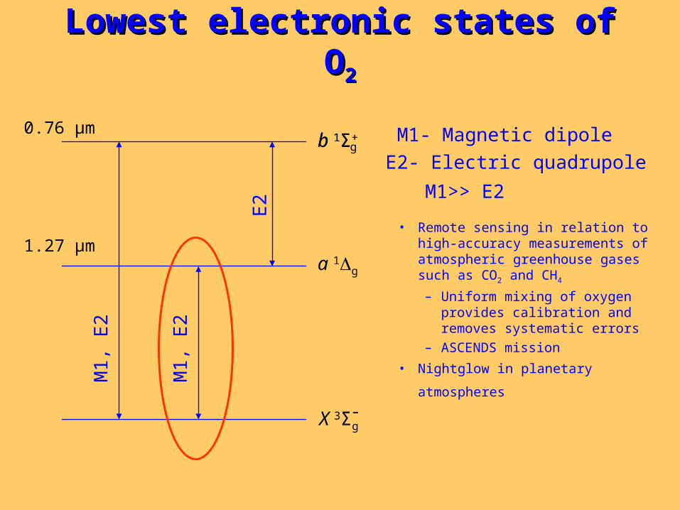
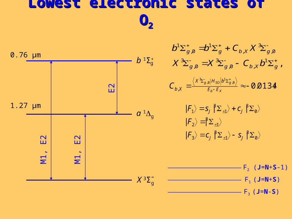
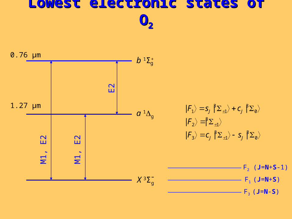
Lowest electronic states of OLowest electronic states of O22

a 1g

X 3Σg-

M1- Magnetic dipole

E2- Electric quadrupole

M1

, E2

M1

, E2

E2

• Remote sensing in relation to high-accuracy measurements of atmospheric greenhouse gases such as CO2 and CH4

– Uniform mixing of oxygen provides calibration and removes systematic errors

– ASCENDS mission

• Nightglow in planetary atmospheres

M1>> E2

1.27 µm

0.76 µmb 1Σ+b 1Σ+

g

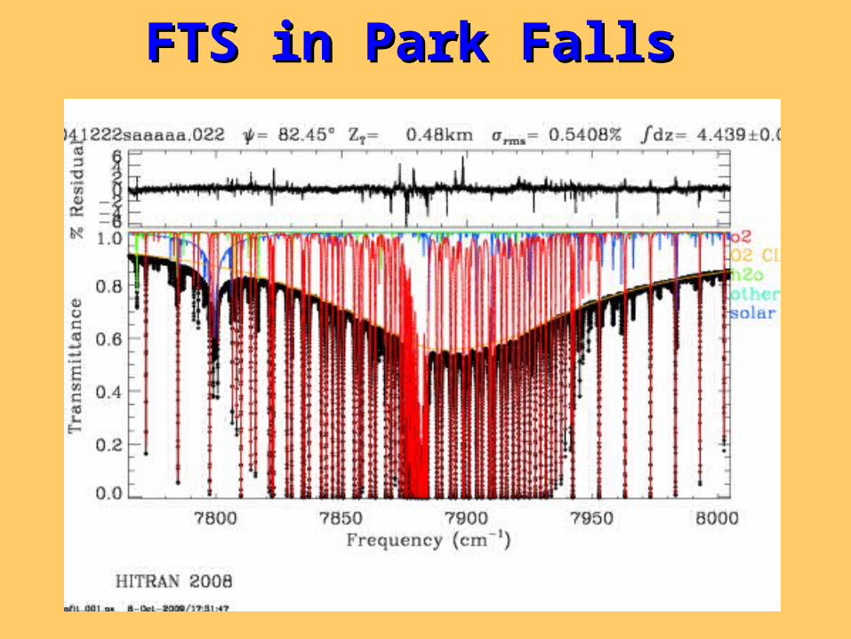
FTS in Park FallsFTS in Park Falls

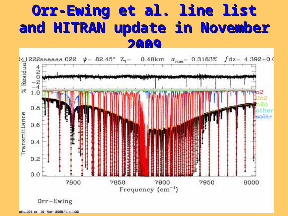
Orr-Ewing et al. line list and HITRAN Orr-Ewing et al. line list and HITRAN update in November 2009update in November 2009

Lowest electronic states of OLowest electronic states of O22

b 1Σ+

a 1g

X 3Σg-

M1

, E2

M1

, E2

E2

F1 (J=N+S)

F2 (J=N+S-1)

F3 (J=N-S)

03

13

3

13

2

03

13

1

|||

||

|||

JJ

JJ

scF

F

csF1.27 µm

0.76 µmg ,1

,0,3

0,3

0,3

,1

0,1

gXbgg

gXbgg

bCXX

XCbb

iCXb

gSOg

EE

bHX

Xb 0134.00,

10,

3

,

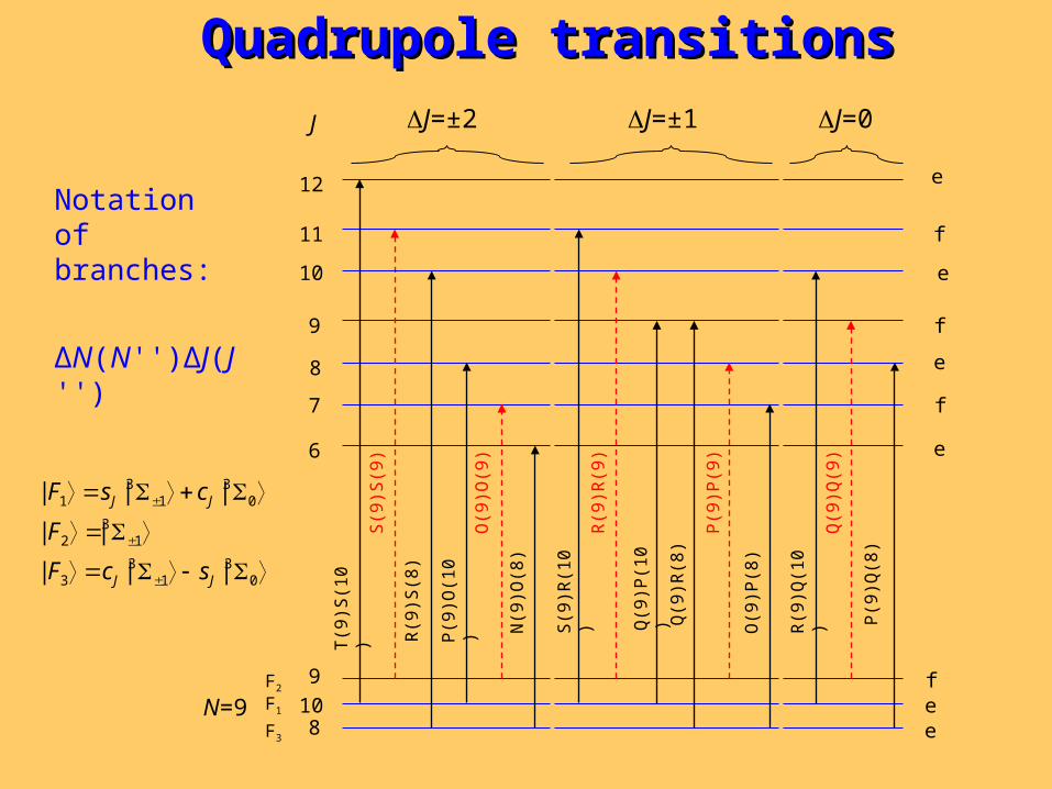
Quadrupole transitionsQuadrupole transitions

8

9

10

8

9

10

11

7

6

12

e

f

e

f

f

e

e

ef

e

J=±2 J=±1 J=0

T(9

)S(1

0)

R(9

)S(8

)

P(9

)O(1

0)

S(9

)S(9

)

O(9

)O(9

)

N(9

)O(8

)

S(9

)R(1

0)

R(9

)R(9

)

P(9

)P(9

)

O(9

)P(8

)

R(9

)Q(1

0)

Q(9

)Q(9

)

P(9

)Q(8

)

J

N=9 F1

F2

F3

Q(9

)R(8

)

Q(9

)P(1

0)

03

13

3

13

2

03

13

1

|||

||

|||

JJ

JJ

scF

F

csF

Notation of branches:

ΔN(N'')ΔJ(J'')

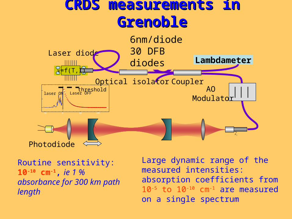
CRDS measurements in GrenobleCRDS measurements in Grenoble

laser ON

-50 0 50 100

Laser diode

Photodiode

Lambdameter

KJ

KJKJKJKJKJ

Optical isolator CouplerAO

ModulatorLaser OFF

threshold

=f(T,I)

6nm/diode30 DFB diodes

Routine sensitivity:10-10 cm-1, ie 1 % absorbance for 300 km path length

Large dynamic range of the measured intensities: absorption coefficients from 10-5 to 10-10 cm-1 are measured on a single spectrum

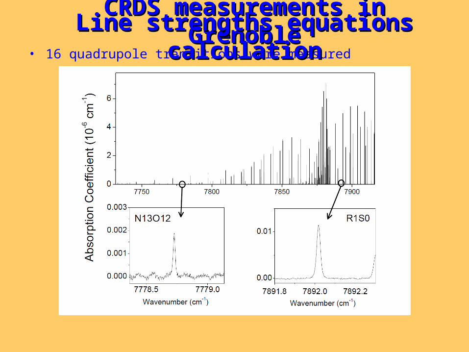
CRDS measurements in GrenobleCRDS measurements in Grenoble• 16 quadrupole transitions were measured

Line strengths equations Line strengths equations calculationcalculation

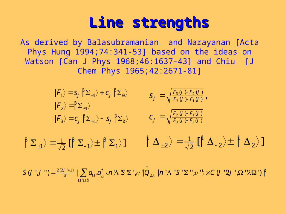
Line strengthsLine strengths

,)()(

)()(

13

23

JFJF

JFJFJs

)()(

)()(

13

12

JFJF

JFJFJc

03

13

3

13

2

03

13

1

|||

||

|||

JJ

JJ

scF

F

csF

]||[| 13

13

21

13

]||[| 21

21

21

21

22

~

'"

*''3

)1''2(2 |)''','2''('',''''''''||',''''|)'','('

JJCSnQSnaaJJS J

As derived by Balasubramanian and Narayanan [Acta Phys Hung 1994;74:341-53] based on the ideas on Watson [Can J Phys 1968;46:1637-43] and Chiu [J Chem Phys 1965;42:2671-81]

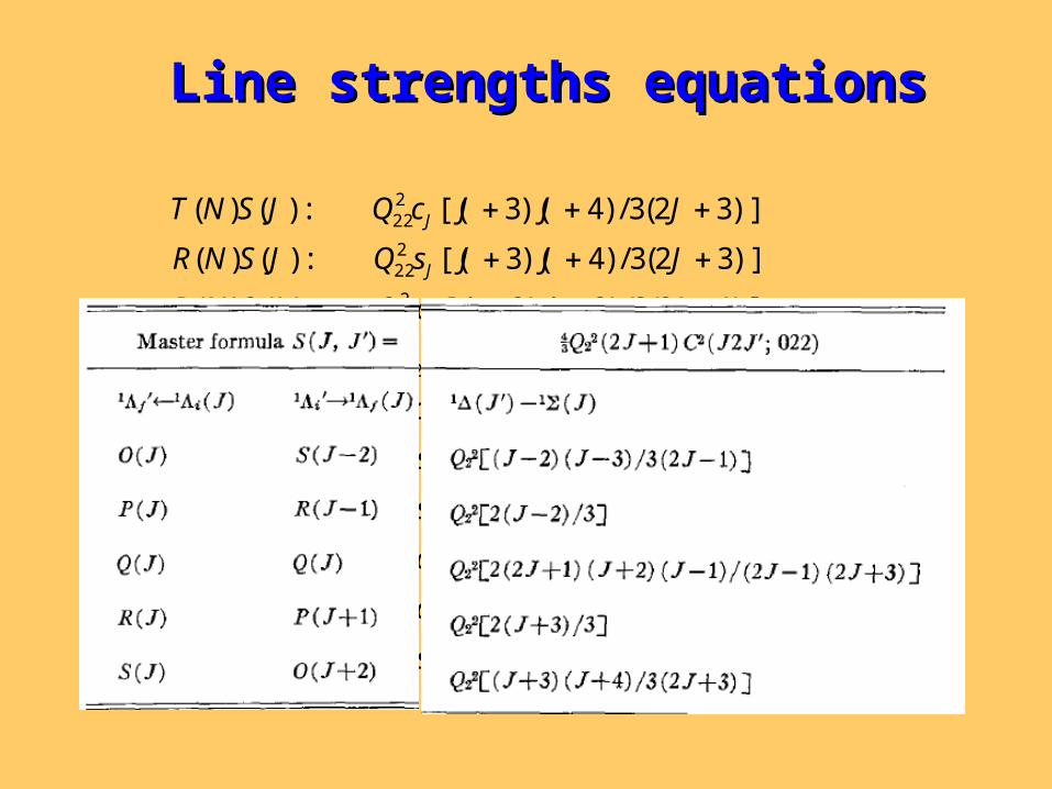
)]32)(12/()1)(2)(12(2[:)()(

)]32)(12/()1)(2)(12(2[:)()(

]3/)2(2[:)()(

]3/)2(2[:)()(

]3/)3(2[:)()(

]3/)3(2[:)()(

)]12(3/)3)(2[(:)()(

)]12(3/)3)(2[(:)()(

)]32(3/)4)(3[(:)()(

)]32(3/)4)(3[(:)()(

222

222

222

222

222

222

222

222

222

222

JJJJJsQJQNP

JJJJJcQJQNR

JcQJPNQ

JsQJPNO

JsQJRNQ

JcQJRNS

JJJsQJONN

JJJcQJONP

JJJsQJSNR

JJJcQJSNT

J

J

J

J

J

J

J

J

J

J

Line strengths equationsLine strengths equations

Quadrupole line list calculationQuadrupole line list calculation

7700 7750 7800 7850 7900 7950 8000 8050 8100

2.0x10-29

4.0x10-29

6.0x10-29

8.0x10-29

1.0x10-28

1.2x10-28

1.4x10-28

1.6x10-28

1.8x10-28

2.0x10-28

N(13)O(12)

P(5)O(6)

R(11)S(10)

T(11)S(12)

R(1)S(0)

Inte

nsi

ty, c

m-1/(

mo

lecu

le c

m-2)

Wavenumber, cm-1

N(N)O(J) P(N)O(J) R(N)S(J) T(N)S(J) Experiment

Details of the calculations are given in Gordon et al (JQSRT 111 (2010) 1174–1183)

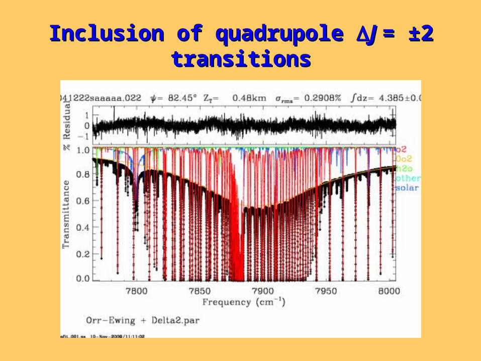
Inclusion of quadrupole Inclusion of quadrupole J J = ±2 = ±2 transitionstransitions

7650 7700 7750 7800 7850 7900 7950 8000 8050 8100 8150

0

1x10-28

2x10-28

3x10-28

4x10-28S

, cm

/mo

lecu

le

Wavenumber, cm-1

J=±2

J=0,±1

JJ=0,±1 and=0,±1 and JJ==±±22

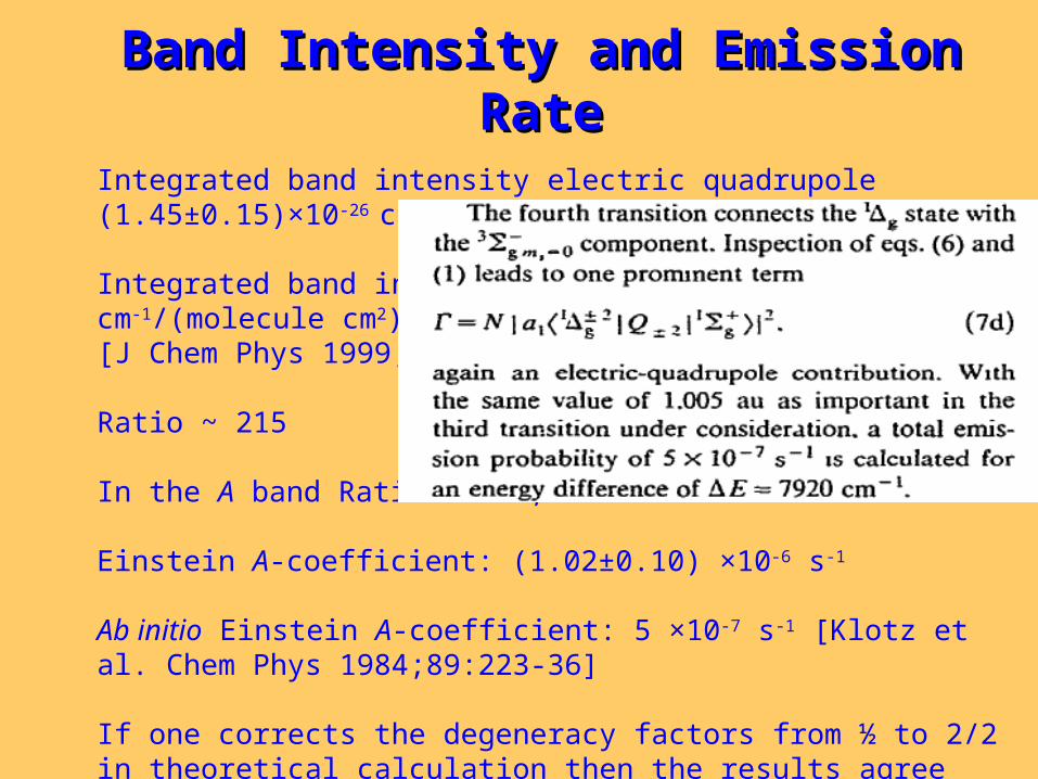
Band Intensity and Emission RateBand Intensity and Emission Rate

Integrated band intensity electric quadrupole (1.45±0.15)×10-26

cm-1/(molecule cm2)

Integrated band intensity (3.10±0.10) ×10-26 cm-1/(molecule cm2)[J Chem Phys 1999;110:10749–57]

Ratio ~ 215

In the A band Ratio ~ 120, 000

Einstein A-coefficient: (1.02±0.10) ×10-6 s-1

Ab initio Einstein A-coefficient: 5 ×10-7 s-1 [Klotz et al. Chem Phys 1984;89:223-36]

If one corrects the degeneracy factors from ½ to 2/2 in theoretical calculation then the results agree very well

Lowest electronic states of OLowest electronic states of O22

b 1Σ+

a 1g

X 3Σg-

M1

, E2

M1

, E2

E2

F1 (J=N+S)

F2 (J=N+S-1)

F3 (J=N-S)

03

13

3

13

2

03

13

1

|||

||

|||

JJ

JJ

scF

F

csF1.27 µm

0.76 µmg

AcknowledgementsAcknowledgements

• J.-F. Blavier, R. Washenfelder, P. Wennberg

• A. Orr-Ewing

• R. W. Field

• S. Yu

• NASA and ANR

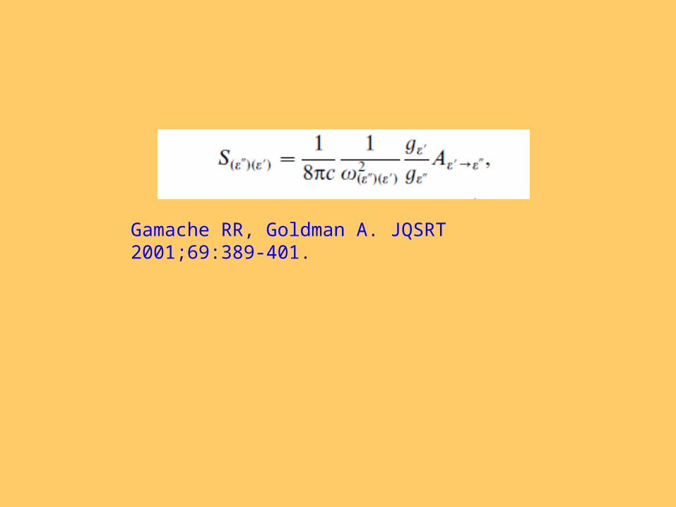
Gamache RR, Goldman A. JQSRT 2001;69:389-401.