Elec4622: Multimedia Signal Processing Chapter 2: Multi ... · °c Taubman, 2003 Elec4622:...

Elec4622: Multimedia Signal ProcessingChapter 2: Multi-Dimensional LSI Filters

Dr. D. S. Taubman

August 22, 2007

1 FIR Filters

1.1 Definition

The unit impulse sequence, δ[n], is defined by

δ[n] =

(1 if n = 0

0 otherwise.

Recall that the boldface n is actually an m-dimensional vector of integer-valued position coordinates. For images, m = 2 so that

n =

µn1n2

¶with n1 the row index and n2 the column index. For video, m = 3, so that

n =

⎛⎝ n1n2n3

⎞⎠with n1 the row index, n2 the column index and n3 the frame (or slice)number.

Let h[n] be the response of a Linear Shift Invariant (LSI) filter δ[n]. Wecall this the filter’s impulse response. By shift invariance, the response to aunit impulse located at k (i.e. the response to the signal, δ[n− k], must bea shifted copy of h[n], i.e. h[n− k]. Now an arbitrary input sequence, x[n],may be represented as a sum of scaled, shifted impulses, i.e.

x[n] =Xk

δ[n− k] · x[k]

1

c°Taubman, 2003 Elec4622: Multi-Dimensional LSI Filters

and so by linearity, the output of the filter, y[n], must be the sum ofweighted, shifted impulse responses, i.e.

y[n] =Xk

h[n− k] · x[k] (1)

The above operation is termed “convolution”. We will often use the conve-nient symbolic notation:

y [n] = (h x) [n]

It is best to avoid expressions like h [n] x [n], which is meaningless if youconsider that h [n] and x [n] are just isolated signal values at a particularlocation n; expressions like that can generate a lot of confusion when thecontext becomes more complex.

By changing the variable of summation, we easily see that convolutionis a symmetric operator, with

y[n] = (x h) [n] =Xk

h[k] · x[n− k] (2)

Accordingly, we may either think of convolving the multi-dimensional signalx [n] with h[n], or convolving the filter’s impulse response with the multi-dimensional signal, x[n]. The distinction between the filter and the signalis immaterial from the perspective of the convolution equation, but not inpractice. In practice, we expect the filter to have a small region of supportin comparison to the signal.

The region of support is the set Rh, of points n, at which the impulseresponse is non-zero, i.e.

h[n] 6= 0⇐⇒ n ∈ Rh

Finite Impulse Response (FIR) filters are those for which the set, Rh, hasfinitely many elements. These are the most simple to understand and imple-ment since the convolution equation (2) may be implemented directly withkRhk additions and multiplications for each output sample.

By contrast, Infinite Impulse Responses (IIR) have infinite regions ofsupport. Nevertheless, there is a limited class of IIR filters which can beimplemented with finite computation — this is the class of filters for whichstable recursive implementations exist. IIR filters are used much less fre-quently for multi-dimensional signal processing applications than in 1-D.One undesirable property of IIR filters that renders them less interestingin multiple dimensions is that they cannot generally have linear phase. As


we shall see in Section 1.5, linear phase is a very important property whenprocessing visual media. For these reasons, we will largely ignore IIR fil-ters during this course, except in a few special circumstances such as splineinterpolation and recursive averaging of video frames.

1.2 Inner Product Notation

The filtering operation (convolution) is often expressed in a different way,which can provide additional insight into what is going on. Consider theset X of all sequences x[n]. This forms an infinite dimensional vector spacewhose analogy with the more familiar finite dimensional vector spaces suchas 2-D and 3-D space is often helpful. Each sequence corresponds to a vector,which we might write as x ∈ X , where x[n] identifies the nth coordinate ofthe vector x. The vectors x satisfy all the usual vector space properties:

• Addition and scalar multiplication are defined point-wise so that wewrite x+y for the sequence whose values are x[n] + y[n] and α ·x forthe sequence whose values are α · x[n].

• The zero vector, 0, is the sequence whose values are all zero.• The inner product between two vectors is written hx,yi and definedby

hx,yi =Xn

x[n]y[n]∗ (3)

where a∗ denotes the complex conjugate of a (no effect on real-valuedsequences).

• The norm (length) of a vector is written kxk and defined by

kxk2 = hx,xi =Xn

kx[n]k2

Note that Cauchy’s inequality holds, i.e. 0 ≤ hx,yi ≤ kxk · kyk andwe define the angle, θ, between two vectors according to

cos(θ) =hx,yikxk · kyk

by analogy with the familiar geometric vector spaces. Two vectors, xand y, are said to be orthogonal if hx,yi = 0. They are said to beorthonormal if they are orthogonal and both have unit length, kxk =kyk = 1.


• We say that a family of vectors, yk, spans the space of all vectors, x, ifeach x may be written as a linear combination of the yk. We say thatthe yk form a basis if this linear combination is unique; equivalently,the vectors, yk, are linearly independent. We say that the yk forman orthonormal basis if hyk1 ,yk2i = 0 for k1 6= k2 (orthogonality) andkykk = 1 for each k. If the yk are an orthonormal basis then eachvectors, x, may be written as a sum of its projections onto the basisvectors, i.e.

x =Xk

yk · hx,yki (4)

Convolution may also be rewritten in terms of inner products, as definedin equation (3). To this end, let h denote the reversed, conjugated sequence,h[n] = h[−n]∗. We will frequently use this notation “conjugate flipping” ofa sequence. Then the convolution formula may be written:

y[n] =Xk

x[k]h[n− k]

=Xk

x[k]h∗[k− n]

= hx, hni (5)

where ad denotes the sequence formed by shifting a by d, so that ad[n] =a[n − d]. In many ways the above formula for convolution is more easilyvisualized. The following steps are involved:

1. Flip the LSI filter’s impulse response, conjugating the terms if neces-sary (only for complex-valued filters).

2. For each location n in the output, determine y[n] by translating theflipped impulse response to location n (think of sliding a mask) andthen take the inner product between the two sequences (think of ap-plying the mask).

This is quite intuitively understood in terms of applying a moving win-dow or mask.

1.3 Separability

The 2-D impulse response, h[n], (or any arbitrary 2-D sequence), is said tobe separable if

h[n] = h1[n1] · h2[n2]


The definition extends in the obvious way to signals in more than two di-mensions. Separable impulse responses are particularly convenient from animplementation standpoint because y[n] may be obtained from a cascade ofone-dimensional filtering steps as follows:

y0[n] =Xk

h1[k] · x[n1 − k, n2]

y[n] =Xk

h2[k] · y0[n1, n2 − k]

To see how this represents a computational advantage, suppose h[n] isa two dimensional PSF with a rectangular region of support, Rh =[A1, B1] × [A2, B2]. The direct implementation of the filter would requireapproximately (B1 − A1 + 1)(B2 − A2 + 1) multiplications and additionsfor each output pixel, whereas the separable implementation requires only(B1 − A1 + 1) + (B2 − A2 + 1). The difference can be very substantial forfilters with large impulse responses.

1.4 Boundaries

Although we will frequently treat images as infinite two-dimensional se-quences of samples, real images have only finite extent. Video sequenceshave finite extent at least in the two spatial dimensions, while volumes havefinite extent in all three dimensions. Since filter impulse responses havespatial extent, the question naturally arises as to how boundaries should betreated. Suppose the real image x[n] is defined over n ∈ [0, N1−1]×[0, n2−1]and that we want the output, y[n], over the same region. The following fourboundary extension techniques cover common practice:

Zero Padding: In this, the simplest case, we simply assume that x[n] = 0for n /∈ [0, N1 − 1] × [0, N2 − 1] when implementing the convolutionequation (2). Although simple, this extension policy has two maindrawbacks:

• Firstly, it should be noted that many image processing operationsare based either explicitly or implicitly on assumptions concern-ing the statistical properties of the image sequence x[n]; the stepedges introduced by setting the sequence to zero everywhere out-side the known region, usually violate these statistical assump-tions, resulting in unpleasant artifacts at image boundaries. Forexample, suppose that we are trying to remove some optical or


motion-induced image blur. The sharpening filter which we con-struct will be based on the assumption that the image is blurredso that sharp transients cannot exist. The zero padding oper-ation will clearly violate this assumption at image boundaries,resulting in unpleasant ringing artifacts near the boundaries.

• Secondly, and perhaps more seriously, the zero padding conven-tion renders the filtering operation sensitive to level shifts. Inmany applications, the impulse response has unit DC gain, i.e.Pn h[n] = 1, so that the operation is insensitive to shifts in the

amplitude level of the input, i.e. y = h x⇐⇒ y+a = h (x+a),where a is an amplitude offset. The zero padding convention de-stroys this property so that level shifts introduce artifacts nearthe image boundaries. This problem can be overcome by replac-ing missing samples beyond the boundary by the image meanamplitude, but the alternative extension policies described beloware preferable to a global solution of this form.

Periodic Extension: In this case, the image is treated as a single periodof a periodic signal with infinite extent, defined by x[n1, n2] = x[n1 +k1N1+k2N2], for all integers, k1 and k2. Clearly, this solves the secondproblem associated with zero padding, in that the policy preserveslevel shifts. However, it generally introduces sharp step edges at theboundaries, with exactly the same consequences as the zero paddingapproach. Even worse, periodic extension brings information fromopposite edges of the image together, so that even filters with smallimpulse responses will mix some information from the right of theimage into the output at the left of the image and vice versa, which ishighly undesirable. Nevertheless, periodic extension can be convenientwhen working with discrete Fourier transforms, as we shall see.

Zero Order Hold: In this case, missing pixels are simply replicated fromthe nearest boundary pixel. So, on the left boundary we havex[−n1, n2] = x[0, n2], n1 > 0; on the right boundary we havex[N1−1+n1, n2] = x[N1−1, n2], n1 > 0; and so on. Pixel replicationavoids many of the problems associated with zero padding, but thestatistical properties of the extended boundary are still significantlydifferent from those of a natural image. The symmetric extension pol-icy described below largely solves this problem.

Symmetric Extension: In this case the missing pixels are obtained bymirroring the image about its boundaries. So, for example, pixels


missing to the left of the image may be set to x[−n1, n2] = x[n1, n2] orx[−n1, n2] = x[n1− 1, n2] for n1 > 0. The former expression is termed“odd” symmetric extension, whereas the latter is termed “even” sym-metric extension. Similarly, at the right hand boundary, the odd andeven extensions are, respectively, x[N1−1+n1, n2] = x[N1−1−n1, n2]and x[N1 − 1 + n1, n2] = x[N1 − n1, n2] for n1 > 0.

It is not hard to show that all these boundary extension policies areseparable, in the sense that they may be applied first in the horizontaldimension, extending each row as far as necessary, and then to the verticaldirection, extending the horizontally extended image rows, or vice versa.

1.5 The Importance of Linear Phase

Recall that the Discrete Space Fourier Transform (DSFT) of the m-dimensional PSF h [n] is defined over the Nyquist volume [−π, π]m by

h (ω) =Xn

h [n] e−jωtn, ω ∈ [−π, π]m

We say that h[n] has zero phase if h(ω) is real-valued, i.e. arg(h(ω)) = 0. Inthe space domain, this is equivalent to requiring the PSF to be symmetricabout the origin, i.e. h[n] = h[−n].

More generally, consider the DSFT h(ω) = h0(ω)e−jstω, where h0[n] is

the PSF of a zero-phase filter and s is a real valued m-dimensional vector(we shall see that it corresponds to a shift). We call this a linear phaseresponse because

arg(h(ω)) = ωts =mXi=1

ωisi

is a linear function of the frequency coordinates ωi. Now let h(x) be the in-verse continuous-space Fourier transform of h(ω), taking the response to bezero outside the region, [−π, π]2, on which the DSFT is defined. We showedin Chapter 1 that h[n] is simply a sampled version of h(x); specifically,

h[n] = h(x)|x=nSimilarly, h0[n] = h0(x)|x=n, where h0(x) is obtained by taking the inversecontinuous-space Fourier transform of the zero-phase filter’s DSFT, h0(ω).But the linear phase term is equivalent to a shift in the continuous-spacedomain so that

h[n] = h(x)|x=n = h0(x− s)|x=n = h0(x)|x=n−s


This shows that the linear phase filter h[n], is just a sampling of the sameunderlying zero-phase continuous signal h0(x) ≡ h0[n]; however, the sam-pling locations are shifted by s (for images, they are shifted down by s1and to the right by s2). To complete our analysis of linear phase filters,we need only recognize that the shifting operation is itself an LSI operator,with Fourier transform e−jωts. Accordingly, a shift in the filter’s impulseresponse is equivalent to shifting the input signal instead. The shift need notbe an integer number of pixels. Thus, a linear phase filter has essentially thesame properties as a zero phase filter, except that it represents an additionalshift by some amount which is generally a fractional number of pixels.

Linear phase filters turn out to be extremely important in image process-ing, because the Human Visual System (HVS) is very sensitive to phase. Asmentioned above, linear phase and zero phase properties have similar impactupon the visual appearance of an image (apart from a shift). Filters withnon-linear phase response, however, tend to introduce very disturbing arti-facts. To see this, suppose that h[n] is an arbitrary non-linear phase filterand let h0[n] be the zero phase filter obtained by setting h0(ω) = kh(ω)k.Then h(ω) = h0(ω)e

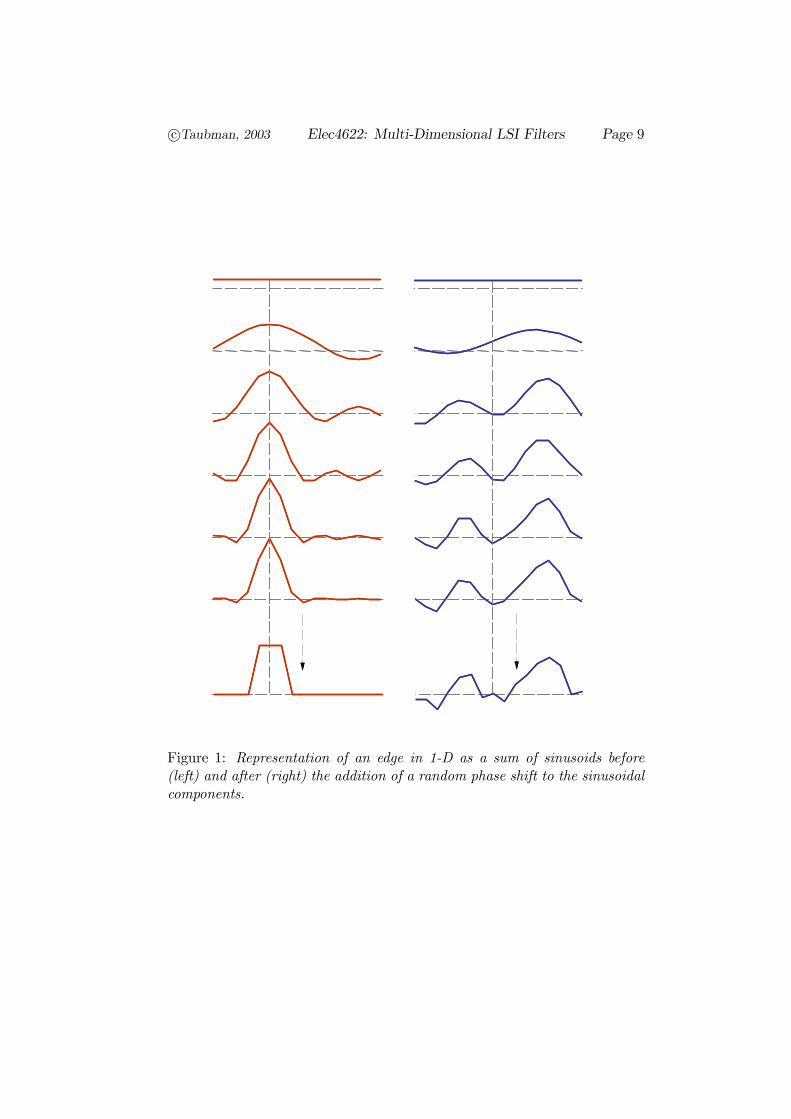
−jφ(ω), where e−jφ(ω) = exp(−j arg(h(ω))) is the non-linear phase term. The effect of the zero-phase component is to selectivelyattenuate different spatial frequencies, whereas the effect of the phase term isto selectively shift different frequency components of the signal. The inverseDSFT represents the original signal as a sum of sinusoids at frequencies ω.If these sinusoids are shifted by different amounts then edges in the imagewill be destroyed. Figure 1 illustrates this effect in one dimension.

2 Filter Implementation

Broadly speaking, we may classify filter implementation strategies into directspatial domain implementations and FFT-based implementations. In thissection, we are concerned only with spatial domain filtering. FFT-basedimplementations are considered in Chapter 4.

2.1 Input and Output Based Approaches

With regard to direct implementation, we can consider two complementaryapproaches. The first approach derives from the convolution equation (1),which recognizes the output signal as a weighted superposition of translatedPSF’s. Writing y as the vector containing all samples of the output sequencefor y [n], h as the vector containing all samples of the filter’s point spreadfunction h [n], and hk for the PSF translated by k (i.e., h [n− k]), the


Figure 1: Representation of an edge in 1-D as a sum of sinusoids before(left) and after (right) the addition of a random phase shift to the sinusoidalcomponents.


convolution equation states that

y =Xk

x [k] · hk

The following algorithm embodies the natural implementation of this equa-tion:

Step 1: Create a block of memory (an array) to hold the output image yand initialize its contents to y = 0.

Step 2: Create a second block of memory (an array) to hold the PSF h. Ina native programming language like "C", you can arrange for this arrayto be represented in your program by a pointer to the element withindex n = 0, in which case your implementation can closely reflect theappearance of the convolution equation.

Step 3: For each location k in the input image, shift h by k, scale its con-tents by the value of the input image at location k (i.e., by x [k]) andadd the result into the output buffer, y. As for practical implemen-tation, we don’t need to physically shift h around in memory, we justneed to adjust our indices so that:

For each location n in the output image, such that n−k falls withinRh, the region of support of the PSF h, we perform the followingassignment:

y [n]← y [n] + x [k] · h [n− k] (6)

We refer to this implementation strategy as “input-based,” since we walkthrough each sample in the input sequence, adding its contribution progres-sively into the evolving output image, y.

The second approach derives from the inner-product formulation of equa-tion (5), which recognizes that each output sample y [n] may be obtaineddirectly as the inner product between the input image x and the mirrorimage of the PSF, h, translated by n. The corresponding algorithm may beexpressed as follows.

Step 1: Create a block of memory (an array) to hold the mirror image PSFh. Again, in a native programming language like "C", you can arrangefor this array to be represented in your program by a pointer to theelement with index n = 0.


Step 2: For each location n in the output image, shift h by n and takethe inner product with x. Again, we don’t need to physically shift haround in memory, we just need to adjust our indices so that

y [n]←Xi∈Rh

h [i] · x [n+ i] (7)

One way to think about this is that y [n] is being formed from a linearcombination of the input samples in the neighbourhood about x [n],where the locations i which lie in the region of support of h are thedisplacements from location n to each sample in this neighbourhood.

We refer to this implementation strategy as “output-based,” since we walkthrough each sample in the output sequence, forming it directly by takinga linear combination of the relevant input samples.

Some reflection should reveal that the input-based and output-basedapproaches ultimately involve exactly the same computations, so that thetotal computational cost is identical. However, the input-based approachrequires additional memory access operations.

• In the output-based approach equation (7) requires exactly °°Rh

°° =kRhk memory reads and one memory write for each location in theoutput sequence.

• In the input-based approach, each location k in the input sequenceinvolves one memory read (to find x [k]) followed by kRhk applicationsof equation (6), each of which involves two reads (for h [n− k] and thecurrent value of y [n]) and a write (for the updated value of y [n]).

In conclusion, the output-based approach is almost always preferable tothe input-based approach. Nevertheless, some exceptions may arise. In theevent that we have a relatively small input sequence, which is understood tobe extended with an infinite number of zeros on all boundaries1, the input-based approach has the potential benefit that computation is bounded bythe number of input samples. Conversely, if we are only interested in asmall region in the output signal, the output-based approach is naturallyfavoured. In most cases, we are ultimately interested in producing filteredsignals with the same dimensions as the original input signals.

1Of course, this happens only in rare applications, since zero padding is one of the leastdesirable boundary extension policies, as discussed in Section 1.4.


output image

input image boundary extension

input window (stripe)

output stripe

h~

output image

input image boundary extension

input window (stripe)

output stripe

h~

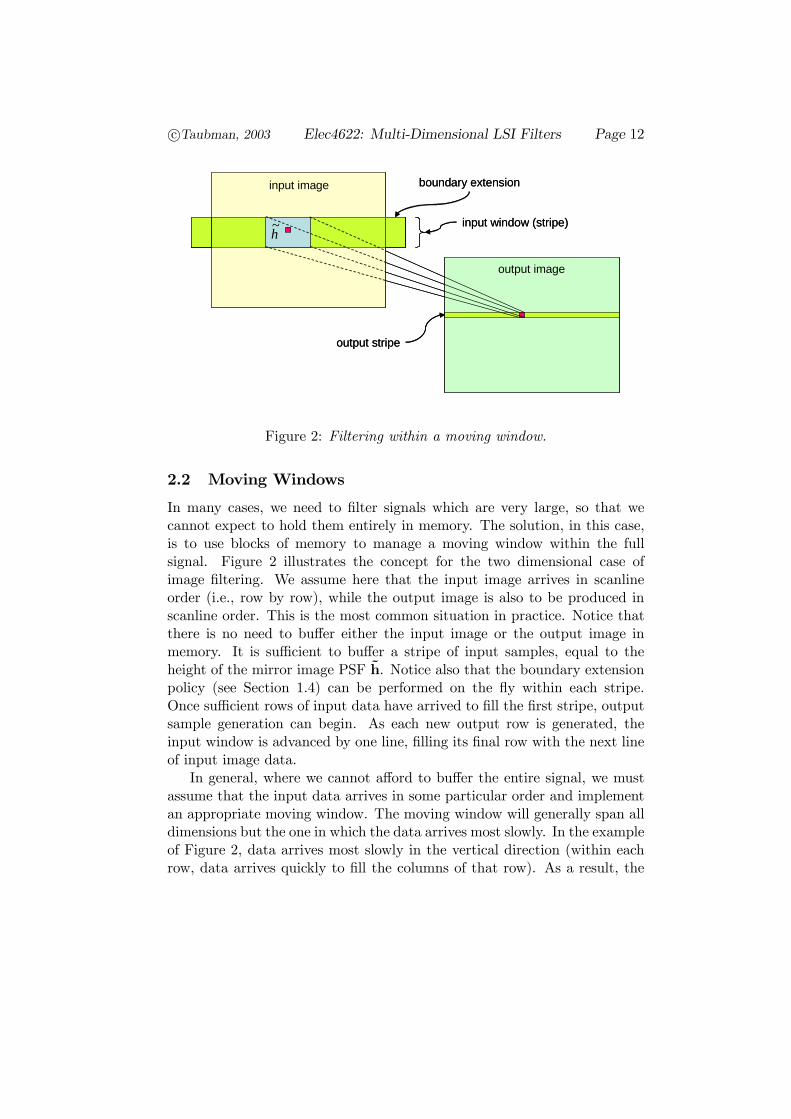
Figure 2: Filtering within a moving window.

2.2 Moving Windows

In many cases, we need to filter signals which are very large, so that wecannot expect to hold them entirely in memory. The solution, in this case,is to use blocks of memory to manage a moving window within the fullsignal. Figure 2 illustrates the concept for the two dimensional case ofimage filtering. We assume here that the input image arrives in scanlineorder (i.e., row by row), while the output image is also to be produced inscanline order. This is the most common situation in practice. Notice thatthere is no need to buffer either the input image or the output image inmemory. It is sufficient to buffer a stripe of input samples, equal to theheight of the mirror image PSF h. Notice also that the boundary extensionpolicy (see Section 1.4) can be performed on the fly within each stripe.Once sufficient rows of input data have arrived to fill the first stripe, outputsample generation can begin. As each new output row is generated, theinput window is advanced by one line, filling its final row with the next lineof input image data.

In general, where we cannot afford to buffer the entire signal, we mustassume that the input data arrives in some particular order and implementan appropriate moving window. The moving window will generally span alldimensions but the one in which the data arrives most slowly. In the exampleof Figure 2, data arrives most slowly in the vertical direction (within eachrow, data arrives quickly to fill the columns of that row). As a result, the


moving window must span the horizontal dimension. In the case of videofiltering, the data normally arrives most slowly in the temporal dimension(i.e., frame by frame), so the moving window must span both the spatialdimensions, having finite support in the temporal direction (i.e., we muststore a finite number of frames).

In Figure 2, we have illustrated the moving window concept for theoutput-based processing paradigm. We could instead adopt the input-basedprocessing paradigm, in which case the moving window would be main-tained within the output signal — see if you can work out how this would beimplemented.

2.3 Separable Filters

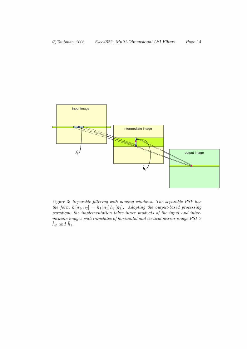
As noted in Section 1.3, separable filters can be implemented as a cascade ofone-dimensional filtering operations, along each of the dimensions in turn.Thus, for images, one filters first in the horizontal direction and then filtersthe result in the vertical direction, or vice-versa. Thus, it is best to thinkabout anm-dimensional filter as a cascade ofm separate filtering operations,withm−1 intermediate results. Each of these individual filtering operationscan then be implemented using the techniques described above.

In order to avoid excessive buffering of intermediate results, the movingwindow strategy of Section 2.2 should be employed, at least at the interme-diate stages. This is illustrated in Figure 3 for the case of separable imagefiltering. In the figure, the horizontal filtering step is performed first, fol-lowed by vertical filtering. Note that there is no need to store the entireintermediate image. Only the vertical processing window need occupy phys-ical memory. As suggested by the figure, the horizontal filter serves to fillthe final row in the intermediate image stripe. Previous rows in this stripebuffer hold results computed previously by the horizontal filtering stage.

2.4 Numerical Representations

Before concluding our introductory treatment of filter implementation, wepause to consider how the sample values should be represented. In the sim-plest case, a floating point representation may be used for each sample value.This is simplest, since the filter coefficients normally have non-integer values.However, floating point numbers typically consume 4 bytes each, whereasthe original sample values might be represented at much lower precision —e.g., as 8-bit numbers. The adoption of a floating point representation incursthe following penalties:


output image

intermediate image

1~h

input image

2~h output image

intermediate image

1~h

input image

2~h

Figure 3: Separable filtering with moving windows. The separable PSF hasthe form h [n1, n2] = h1 [n1]h2 [n2]. Adopting the output-based processingparadigm, the implementation takes inner products of the input and inter-mediate images with translates of horizontal and vertical mirror image PSF’sh2 and h1.


1. More memory is required to implement working buffers. This maybe completely irrelevant for one dimensional signal processing, butremember that moving windows used in multi-dimensional filteringmust fully span all but one of the dimensions.

2. More byte transactions are required between memory and the compu-tational processing engine in order to complete the filtering process.Memory bandwidth is often a more critical resource than the actualamount of memory, since technological advances have seen memorysize advance much more rapidly than memory bandwidth.

3. Conversion between floating point and integer representations can bequite computationally intensive. This is important if the input se-quence originally has an integer representation or the output sequenceis required to have an integer representation, as is often the case.

4. Numerical computation involving floating point quantities is morehardware intensive than the corresponding operations performed usinginteger arithmetic. This is particularly true in the case of additions.Integer addition is trivial, whereas each floating point addition opera-tion must be followed by a potentially tedious renormalization step.

5. Numerical computation with floating point quantities involves round-ing errors which are hard to model mathematically. This can makeit difficult to guarantee the performance of an implementation overall possible input conditions, even though numerical errors are usu-ally smaller with floating point arithmetic than can be achieved withsimilar sized integer representations.

In view of the above considerations, we must be prepared to implementour filters using all integer arithmetic. for simplicity, let us suppose thateach input sample x [n] and each output sample y [n] is to be represented asa B-bit two’s complement signed integer. This means that

−2B−1 ≤ x [n] , y [n] < 2B−1

Since our filter coefficients are typically non-integer valued, we need to firstrecognize that rounding will be involved. Adopting the output-based for-mulation, we can write this as

y [n] =

*Xi∈Rh

h [i]x [n+ i]

+


Here, we are using the notation hi for rounding to the nearest integer. Wecan rewrite this as

y [n] ≈*P

i∈RhH [i]x [n+ i]

2P

+, where H [i] =

D2P · h [i]

E(8)

That is, we first scale all the filter coefficients up by some amount 2P andround them to integers, where P ∈ N is the implementation precision. Wethen implement the filtering operation using all integer arithmetic with theH [i] coefficients. The final result needs then to be divided by 2P androunded to the nearest integer again.

In most cases, increasing P improves the accuracy of the approxima-tion represented by the above equation. On the other hand, as P in-creases, so does the precision of the integer arithmetic used to computePi∈Rh

H [i]x [n+ i]. Interestingly, we do not need to worry about the pos-

sibility of numerical overflow as the intermediate results H [i]x [n+ i] areprogressively accumulated. So long as the final sum is guaranteed to fit intothe integer representation adopted for computation, we can be sure that anytemporary overflow or underflow will cancel — this is a useful property of in-teger arithmetic. To ensure that the final sum fits within the selected inte-ger representation, we normally perform a Bounded-Input-Bounded-Output(BIBO) analysis. Specifically, we compute the number of bits N required toensure that ¯

¯Xi∈Rh

H [i]x [n+ i]

¯¯ < 2N−1

From the triangle inequality, we get¯¯Xi∈Rh

H [i]x [n+ i]

¯¯ ≤ X

i∈Rh

¯H [i]

¯· |x [n+ i]| ≤ 2B−1 · 2P ·

Xi∈Rh

¯h [i]

¯| {z }

GBIBO

where GBIBO is known as the filter’s BIBO gain. It follows that we can pickN = B + P + log2GBIBO.

To complete our implementation, we recognize that equation (8) can berewritten as

y [n] ≈$2P−1 +

Pi∈Rh

H [i]x [n+ i]

2P

%


where bxc denotes the truncation operation, which rounds x down to thenearest integer, no larger than x. Division by 2P followed by truncation isthe mathematical description of what happens when we shift all the bits ofan integer to the right by P . Bit shifting operations like this are very fast; inhardware implementations, bit shifting by a constant amount P is nothingother than a rerouting of the wires which represent the bits — it can be freeof any implementation cost. Our recipe, therefore, is to perform the integercomputation

Pi∈Rh

H [i]x [n+ i] using N-bit arithmetic, add the constant

rounding offset 2P−1, and then discard the least significant P bits of theresult. In software implementations, we normally fix N to be 16 or 32 andadjust P to suit.

3 Filter Design

For many applications, it is natural to specify a filter in the frequency do-main, after which we would like to find the impulse response of an FIR filterwhich matches these specifications as closely as possible. For example, wemight specify a circularly symmetric 2-D low-pass filter by requiring thefollowing specifications to be satisfied by h(ω):(¯

(1− kh(ω)k)¯< δp for kωk < ωp,

kh(ω)k < δs for kωk > ωs.

where ωp < ωs denote the radial frequencies corresponding to the pass- andstop-band respectively, while δp and δs are the required tolerances on thepass- and stop-band magnitude. In addition, we will usually require thatthe filter have zero phase, so that h(ω) = kh(ω)k.

3.1 Windowing

The most natural way to design a 2-D FIR filter is to start with some desiredfrequency response, say hd(ω), which satisfies the requirements imposed bythe application and then to take its inverse Discrete Space Fourier Transform(DSFT). Of course, some numerical approximations will be required in thenumerical integration required to obtain hd[n] from this equation. In general,the result will be a filter with infinite support, so we will need to apply somekind of spatial window function w[n] to obtain

h[n] = w[n] · hd[n]


where the support of the window function Rw is identical to the support ofthe filter we are trying to design, Rh.

Of course, the application of this windowing function modifies the fre-quency domain characteristics and so we will need to check that h(ω) stillsatisfies the original constraints. The relationship between h(ω) and hd(ω)is given by:

h(ω) =1

(2π)2

Z π

−π

Z π

−πdν · w(ν)hd(ω − ν) (9)

That is, the desired frequency response has been convolved with the DSFTof the window function2. Ideally then, the window will have as narrow abandwidth as possible, i.e. kw(ω)k should decay rapidly with increasingkωk. On the other hand, narrow band windows have large spatial supportand vice-versa so we will be constrained by the desired support size, Rh.

Since we are designing a zero phase filter, we will want to use a zerophase window. In this case w(ω) and hd(ω) will both be real-valued and soh(ω) will also be real-valued (zero phase) by equation (9).

Before discussing particular windowing functions, it is sometimes conve-nient to express the window as a spatially continuous function, w(x), wherew[n] = w(x)|x=n. We assume that the window is sufficiently narrow bandthat it is essentially bandlimited to the Nyquist region, ω ∈ [−π, π]2, sothat the spatially continuous Fourier transform of w(x) is identical to theDSFT of w[n]. Thus, we need only be concerned with the properties of thespatially continuous function, w(x).

In the simplest case, the window function is a separable product of 1-Dwindow functions, i.e.

w(t) = w1(x1) · w2(x2)We now give a few examples of 1-D window functions:

Rectangular Window: In this case, we simply set

w(t) =

(1 for |t| < τ ,

0 otherwise.

2Windowing of spatially continuous functions is exactly equivalent to convolution inthe Fourier domain. For the discrete operators here, windowing is equivalent to cir-cular convolution in the Fourier domain. Formally, equation (9) is not valid sincewe have defined w (ω) and h (ω) only over the Nyquist region ω ∈ [−π, π]2. Forcircular convolution, we interpret hd (ω − v) in equation (9) as the wrapped valuehd (mod2π(ω1 − v1),mod2π (ω2 − v2)) where mod2π (x) adds integer multiples of 2π toits argument x until the result lies in [−π, π]. We shall have more to say on frequencywrapping, and Fourier transforms in general, in Chapter 4.


where τ is the parameter which determines the extent of the window.This trivial window is rarely used in practice because its frequencyresponse decays only slowly. Specifically, w(ω) is the sinc function,

w(ω) = 2τsin(ωτ)

ωτ= 2τ sinc(

ωτ

π)

Raised Cosine (or Hanning) Window: In this case we set

w(t) =

(1+cos(πt

τ)

2 for |t| < τ ,

0 otherwise.

It is easy to verify that this function is continuous with all derivativescontinuous. This means that high frequency components are avoided,which minimizes the effective bandwidth of w(ω). It is a useful exercisefor the reader to derive an expression for w(ω).

Hamming Window: This window is a slight modification of the raisedcosine window, obtained by adding a small amount of the rectangularwindow. It has the form:

w(t) =

(0.54 + 0.46 cos(πtτ ) for |t| < τ ,

0 otherwise.(10)

Another 1-D window which is sometimes used is the Kaiser window, butthe Hamming and Hanning windows are used most frequently, except in themost demanding applications.

For some applications, superior results can be obtained by using non-separable windows. For example, when designing a circularly symmetricfilter, a circularly symmetric window function is generally preferable. Inthis case, it is the continuous window function w(x) = w(t)|t=kxk, whichexhibits circular symmetry prior to sampling; circular symmetry makes nosense for sequences. The same 1-D windows mentioned above are typicallyused for w(t) in this formulation.

3.2 Frequency Sampling

The idea behind the frequency sampling technique is to find a finite set offilter tap values, h[n], n ∈ Rh, which minimizes a weighted combination ofthe squared differences between the desired and actual frequency responses,i.e. khd(ω) − h(ω)k, at a finite set of frequency locations (samples), ωk ∈


[−π, π]2, k = 1, 2, . . . ,K. These frequency locations could be distributeduniformly over the Nyquist region [−π, π]2, but we will usually do better toplace more samples in the neighbourhood of critical frequency regions suchas band edges.

We usually want to ensure that the designed filter is zero phase, in whichcase the DSFT at each of our frequency samples may be written as

h(ωk) =Xn∈Rh

h[n]e−jntωk

= h[0] + 2Xn∈R+

h

h [n] cos(ntωk)

Here, R+h is the region of support restricted to the upper half plane, i.e.R+h = {n ∈ Rh|n2 > 0 or (n2 = 0 and n1 > 0)}

Thus Rh = R+h ∪−R+h ∪ {0}.Let h be the (1+kR+h k)-dimensional vector whose elements are h[0] and

h[n] for each n ∈ R+h . We wish to minimize the weighted squared errorexpression

KXk=1

ρ2k

⎛⎜⎝hd(ωk)− h[0]−Xn∈R+

h

h [n] cos(ntωk)

⎞⎟⎠2

=°°°W · hd −W · C · h

°°°2 (11)

Here,

W =

⎛⎜⎜⎜⎝ρ1 0 · · · 00 ρ2 · · · 0...

.... . .

...0 0 · · · ρK

⎞⎟⎟⎟⎠

C =

⎛⎜⎜⎜⎝1 cos

¡nt1ω1

¢ · · · cos¡ntPω1

¢1 cos

¡nt1ω2

¢ · · · cos¡ntPω2

¢...

.... . .

...1 cos

¡nt1ωK

¢ · · · cos¡ntPωK

¢⎞⎟⎟⎟⎠ , with P =

°°R+h °°

h =

⎛⎜⎜⎜⎝h [0]h [n1]...

h [nP ]

⎞⎟⎟⎟⎠ and hd =

⎛⎜⎜⎜⎝h (ω1)

h (ω2)...

h (ωK)

⎞⎟⎟⎟⎠


Minimization of equation (11) is a classic linear algebra problem whosesolution is well known:

h = (CtW 2C)−1CtW 2hd

Note that ρ2k is any positive weight which reflects the relative importanceof matching the desired response at frequency ωk. Doubling the weight atsome frequency sample is equivalent to adding an extra sample at the samefrequency, so it is possible to reduce the density of samples in critical fre-quency regions by increasing the weight associated with a smaller number ofrepresentative samples. This approach can be used judiciously to reduce thedimension of the matrix inverse problem represented by the above equation.

3.3 The Transformation Method

The filter design methods described above have been expressed in terms ofan initial desired frequency response, hd(ω) and so are unable to explicitlycapture the tolerances in the frequency domain constraints that we usuallystart with, as expressed in equation (10). There are a variety of more sophis-ticated techniques which may be used to design filters subject to a particularset of constraints. We only describe one method here, which is known as theFrequency Transformation method. It is also often known as the McClellanTransformation, after the original proposer of the approach.

We start with the assumption that the one-dimensional filter design prob-lem is much easier, which indeed it is. In one dimension, the so-called “Parksand McClellan” design technique, which is based on the “Remez exchange”algorithm, has been known for some time as a method for designing opti-mum 1-D zero phase FIR filters subject to constraints on the tolerances inthe pass- and stop-bands. It is not necessary to understand the details of the1-D design problem to appreciate the Frequency Transformation method.

The idea is to map the 2-D design problem into a 1-D design problemwithout losing the finite impulse response property. The method is relevantonly for zero phase designs. The key observation is that the frequency


response of a 1-D zero phase filter with 2N + 1 taps may be expressed as

h(ω) = h[0] + 2NXn=1

h[n] cos(ωn)

=NXn=0

ancos(ωn)

=NXn=0

bn(cos(ω))n

The last line in this equation is not obvious, but some careful application ofbasic trigonometric properties eventually yields the result. The coefficients,bn, may be found from the an by equating the polynomialsX

n

anCn(x) =Xn

bnxn

where Cn(x) is the sequence of Chebychev polynomials which are foundrecursively from the following:

• C0(x) = 1

• C1(x) = x

• Cn(x) = 2xCn−1(x)−Cn−2(x) for n ≥ 2.Now the 2-D to 1-D mapping of the frequency transform is given by

h(ω) = h(ω)|cosω=μ(ω) =NXn=0

b[n](μ(ω))n

where μ(ω) is the DSFT of a finite support sequence, μ[n], which controlsthe mapping. The designed filter, h[n], must have a finite support becauseit is a sum of the finite support sequences whose DSFT is given by (μ(ω))n;each such sequence is the n-fold convolution of the finite support sequence,μ[n].

The original algorithm proposed by McClellan uses a mapping kernelμ[n], with the following taps:

μ[n] =

⎧⎪⎪⎪⎪⎨⎪⎪⎪⎪⎩−12 if n = 0,14 if n1 = ±1 and n2 = 0,14 if n1 = 0 and n2 = ±1,18 if n1 = ±1 and n2 = ±1.


2ω

1ω

ππ−2ω

1ω

ππ−

Figure 4: Contour plot of ω = cos−1 (μ (ω)) within the Nyquist region,ω ∈ (−π, π)2, for uniformly spaced ω.

whose region of support, Rμ = [−1, 1]2. Suppose for example that we designa 7-tap 1-D filter, so that N = 3. Then the support of h[n] will be [−3, 3]2,i.e. a 7× 7 region. It can easily be seen that μ(ω) is given by

μ(ω) = −12+1

2cosω1 +

1

2cos(ω2) +

1

4cos(ω1 + ω2) +

1

4cos(ω1 − ω2)

= −12+1

2cosω1 +

1

2cosω2 +

1

2cosω1 cosω2

The contours of this mapping are illustrated in Figure 4. The mappingrepresents quite a good approximation to a circularly symmetric function.

In general, the frequency transform method of filter design involves thefollowing steps:

1. Select a transformation kernel, μ[n]. It is possible to design your ownwith specific requirements in mind, but the original McClellan kerneldescribed above is a common choice.

2. Map the 2-D frequency domain specifications on h(ω) back to spec-ification on the 1-D kernel, h(ω). For example, suppose we require|h(ω)k < δs for kωk > ωs, where ωs is the circularly symmetric bound-ary of the stop band for a low-pass filter specification. Then find thelargest value of ω0s such that μ(ω) ≥ cos(ω0s) for all kωk ≥ ωs andthis value of ω0s is the stop band boundary for the 1-D filter design


problem. The tolerances map directly from the 2-D to the 1-D designproblem.

3. Design a suitable 1-D kernel using, for example, the Parks and Mc-Clellan algorithm.

4 Filtering Examples

4.1 Gaussian Filters

A common choice for an image smoothing filter is one whose impulse re-sponse is a Gaussian function, i.e. h[n] = h(s)|s=n, where the spatiallycontinuous impulse response, h(s), is given by

h(s) =1

2πpkGk exp

µ−s

tG−1s2

¶(12)

Here, G is a 2× 2 symmetric positive definite matrix, and kGk is its deter-minant. Thus,

G =

µσ21 σ1,2σ1,2 σ22

¶and

kGk = σ21σ22 − σ21,2 > 0

The normalization in equation (12) is chosen to ensure thatZ Zds · h(s) = 1

so that the spatially continuous impulse response has unit DC gain, whichone would expect from a smoothing filter.

In most cases the off-diagonal term, σ1,2, is zero so that

h(s) =1

2πσ1σ2exp

Ã−12

Ã∙s1σ1

¸2+

∙s2σ2

¸2!!

=1p2πσ21

exp

µ− s212σ21

¶· 1p

2πσ22exp

µ− s222σ22

¶is a separable Gaussian function whose contours have an elliptical cross-section (circular if σ1 = σ2).

However, the σ1,2 term may be used to design arbitrarily rotated ellip-tical cross-sections. To see this, let G0 = diag(σ21, σ

22) be the matrix which


defines an initial impulse response, h0(s), with elliptical cross-section andmajor and minor axes corresponding to the vertical and horizontal axes.Now consider the rotated impulse response, hθ(s), obtained by the coordi-nate transformation, hθ(s) = h0(u)|u=Θs, where

Θ =

µcos(θ) − sin(θ)sin(θ) cos(θ)

¶(13)

It follows that

hθ(s) =1

2πpkG0k exp

µ−s

tΘtG0−1Θs2

¶=

1

2π√Gθ

exp

µ−s

tGθ−1s2

¶where

Gθ = Θ−1G0Θ−t = ΘtG0Θ (14)

Here, we have used the fact that Θ−1 = Θt and kΘk = 1, which are im-portant properties of rotation matrices that we used also in Chapter 1.Expanding equation (14), we see that

Gθ =

µΣ21 Σ1,2Σ1,2 Σ22

¶with

⎧⎨⎩Σ21 = σ21 cos

2 θ + σ22 sin2 θ

Σ22 = σ22 cos2 θ + σ21 sin

2 θΣ1,2 =

¡σ21 − σ22

¢cos θ sin θ

which has the required form.Gaussian filters have the property that their Fourier transform is also a

Gaussian function, i.e.

h(ω) =

Z Zds · e−jstωh(s)

= exp

µ−ω

tGω

2

¶From this expression, it is evident that the continuous impulse response h(s)is not bandlimited, but provided σ21 and σ

22 are sufficiently large, h(ω) should

be very close to zero outside the Nyquist limit, ω ∈ [−π, π]2. In this case,the DSFT of the sampled impulse response, h[n], will be almost identical tothe spatially continuous Fourier transform of h(s). Under these conditions,it is safe to assume that the DSFT of the sampled impulse response isGaussian and also that

Pn h[n] = 1. Similarly, since the spatial impulse


response decays rapidly as knk becomes large, it is safe to simply truncatethe impulse response (i.e. apply a rectangular window) to some suitablylarge region of support.

Gaussian functions have the convenient property that both the spatialand frequency domain representations are real and positive. Also, if weignore the possibility that σ1,2 might not be zero for simplicity, and identifythe horizontal and vertical “spread” of the Gaussian function by σ1 and σ2,respectively, we see that the horizontal and vertical spread in the frequencydomain is given by 1

σ1and 1

σ2, respectively, so that the product of the spatial

and frequency spreads is always exactly equal to 1. These spreads are oftenidentified with resolution or uncertainty, in which case we can say that theproduct of the resolution (uncertainty) in space and frequency is equal to1, regardless of the values of σ1 and σ2. This product plays an analogousrole to the famous “Heisenberg Uncertainty Principle” in Physics. It isfundamental in the sense that there is no other filter for which the productof spatial and frequency resolutions (spreads) is less than 1 — in fact, for allother filters, it is larger than 1.

The Gaussian low-pass filter may be converted to a band-pass filter bymodulating it with a sinusoidal term. For example, modulating by a cosineyields

h(s) =1

2πpkGk cos(stω0) exp

µ−s

tG−1s2

¶and

h(ω) =1

2exp

µ−(ω + ω0)

tG(ω + ω0)t

2

¶+1

2exp

µ−(ω − ω0)

tG(ω − ω0)t2

¶so that the frequency response is the sum of two Gaussian lobes displacedby ω0 and −ω0, respectively. Modulating by a sine function yields a sim-ilar expression, involving the difference between displaced Gaussian lobes.Cosine and sine modulated Gaussians are known as “Gabor functions.”

4.2 Moving Average Filters

When computational demands must be kept to a minimum it is commonto resort to moving average filters for low-pass, high-pass and band-passoperations. The basic moving average filter has the form

h[n] =1

(b1 + 1− a1)(b2 + 1− a2)·(1 for a1 ≤ n1 ≤ b1 and a2 ≤ n2 ≤ b2,

0 otherwise.


This is a low-pass filter, whose frequency response is a sinc function. Thefilter is separable into the row and column filters, h1[n] and h2[n], with

hi[n] =1

b1 + 1− ai·(1 for ai ≤ n ≤ bi,

0 otherwise., for i = 1, 2

The popularity of moving average filters is due to the fact that the compu-tational complexity is independent of the filter’s region of support. Specif-ically, rather than implementing the one-dimensional filters h1[n] and h2[n]directly, the solution can be obtained recursively using the following trivialalgorithm. Let y[n] =

Pk hi[k]x[n − k] be the desired 1-D filter response

and let y0[n] = (bi + 1− ai)y[n]; then it is easy to see that

y0[n+ 1] = y0[n] + x[n+ 1− ai]− x[n− bi]

so that once an initial value from the scaled output sequence has been com-puted directly, each subsequent scaled output value y0[n] requires only twoadditions3. If the filter support bi+1− ai is chosen to be a power of 2 theny[n] may be recovered from y0[n] with the aid of a simple bit-shift operation.For the full two-dimensional filter then, we need to apply the 1-D movingaverage operation separably in the horizontal and vertical directions, so thatthe total computational requirement is 4 additions and one bit-shift opera-tion per sample, regardless of the support of the filter. It should be notedthat the recursive implementation described here may progressively accumu-late round-off errors in floating point implementations — no such problemsarise when the implementation uses integers.

It is possible to construct a high-pass filter by modulating the impulseresponse by (−1)n1 , (−1)n2 or (−1)n1+n2 . It is easy to see that each of theseleads to filters which have the same implementation properties.

A band-pass filter may be constructed either by cascading a low- andhigh-pass moving average filter with appropriate parameters, or by sub-tracting the output from two moving average low-pass filters with differentsupport sizes. Filters of this form with relatively large regions of supporthave been used successfully to band-pass filter frames from a video sequencein order to increase the reliability of subsequent motion estimation opera-tions.

3Actually one addition and one subtraction, but addition and subtraction are consid-ered to be the same operation from a complexity point of view.


4.3 Unsharp Masking

Unsharp masking is perhaps one of the oldest image processing operations.Its origins lie in analogue photographic processing. It is an ad-hoc techniquefor artificially increasing the sharpness of an image x[n] by forming a crudehigh-pass filter. The following steps are involved, at least conceptually, andthese are the steps used in the original photographic processing setting:

Step 1: Form a low-pass filtered version xL[n] by applying the low-passfilter h[n] to x[n], where h[n] has unit DC gain.

Step 2: Form a purely high-pass image by subtracting the low-pass versionfrom the original image, i.e. xH [n] = x[n]− xL[n].

Step 3: Add some amount of the high-pass image back into the originalimage to form an artificially sharpened image, i.e. y[n] = x[n] + α ·xH [n].

It is not hard to see that the above operations are equivalent to theapplication of a single high-pass filter, whose impulse response hs[n] is givenby

hs[n] = δ [n] + α(δ [n]− h[n]) = (1 + α)δ [n]− αh[n]

In practice, unsharp masking may prove computationally attractive whenthe low-pass filter h[n] is particularly simple, e.g. a moving average filter.The sharpening method is parametrized by the value of α which is oftenadjusted interactively. In some adaptive filtering applications, the value ofα is modulated automatically in accordance with some estimate of the localsignal-to-noise ratio, since we would like to sharpen the signal (e.g. edges),but not amplify the noise.

Unsharp masking is still used today, but not always justifiably. Themethod is entirely ad-hoc and neither the low-pass filter h[n], nor the para-meter α, are usually selected based on any specific knowledge of the problem.This is a common characteristic of the methods found in interactive imageediting programs like Adobe Photoshop

R°.

4.4 Temporal Filtering to find a Video Background

We have seen that moving averages allow us to implement filters with verylarge regions of support with almost negligible computation. In two dimen-sions, we can form a moving average over an arbitrary rectangular windowat a cost of only 4 additions per pixel. In video applications, filters with


very large support in time are also sometimes of interest. Perhaps the mostimportant application is that of forming a “background” frame.

Background frames are particularly important in surveillance applica-tions, where the background scene changes only very slowly with time,whereas foreground objects may occasionally transit through the scene. Bysubtracting each successive video frame from a “known” background, it ispossible to identify foreground objects, detect intruders and so forth. Onepossible way of forming a background frame is to use a single image, cap-tured at a time when the scene is known to be free from non-backgroundobjects. The problem with this is that the single fixed background frame isunable to account for the effects of changing lighting conditions and smalldisplacements in the camera.

The next simplest way to form a video background frame is to take amoving average over a long period of time. Following our previous treatmentof moving average filters, we would expect a pure temporal moving averageto have a computational cost of only 2 additions per pixel, while a fullseparable spatio-temporal moving average filter would have a cost of only6 additions per pixel. The problem, however, is that moving average filtersimplemented in this way require the retention of a large number of videoframes in memory — equal to the temporal support of the filter in question.To avoid the high memory cost, it is more common to implement a simplerecursive IIR filter in the temporal direction.

Let xk [n] denote the kth frame in a video sequence, with spatial indicesn ≡ [n1, n2]. Let yk [n] denote the background frame formed at the kth frameinstant. A single-pole recursive filter may be used to form this backgroundframe using

yk [n] = (1− α) · xk [n] + α · yk−1 [n]Using the standard methods of 1D signal processing to analyze this filter,let

Xz [n] =Xk

z−kxk [n] and Yz [n] =Xk

z−kyk [n]

be the temporal Z-transforms of xk [n] and yk [n] respectively and observethat

Yz [n] = (1− α)Xz [n] + αz−1Yz [n]

so that

Yz [n] =(1− α)Xz [n]

1− αz−1= Xz [n]

1− α

1− αz−1| {z }H(z)


This means that the background is formed by applying a single pole filterto the original video content, having a pole at z = α. Substituting z = ejω

we see that the low-pass filter has frequency response

h (ω) = H (z)|z=ejω =1− α

1− αe−jω

The filter has DC gain of 1 and as α approaches 1 (i.e., as the pole approachesthe unit circle), the filter becomes progressively more low-pass in nature. Forα close to 1, it can be shown that the filter’s 3 dB cut-off frequency occursat ω ≈ 1− α.

This recursive filtering approach allows us to achieve arbitrarily largeattenuation of the higher temporal frequency components simply by bringingα close to 1, without increasing the memory storage beyond 2 frames —one frame to hold xk [n] and one to hold the background yk [n], which isupdated in place. One subtle drawback of the approach, however, is thatthe background experiences a large delay. In fact

arg³h (ω)

´= − tan−1

µα sinω

1− α cosω

¶≈ − α

1− αω [for small ω]

≈ 1

1− αω [for α close to 1]

The effective delay, therefore, is approximately 1/ (1− α) frame periods.This means that the background that is being subtracted from a currentframe xk [n] to detect foreground objects may be considerably out of date.To remedy this problem requires the introduction of a large amount of mem-ory, at which point the benefits of IIR filtering over the simple moving av-erage FIR filter are largely lost.

Elec4622: Multimedia Signal Processing Chapter 2: Multi ... · °c Taubman, 2003 Elec4622:...

Documents

Transcript of Elec4622: Multimedia Signal Processing Chapter 2: Multi ... · °c Taubman, 2003 Elec4622:...