Institute of Structural Analysis & Seismic Research

Elastoplastic Constitutive Models

in Finite Element Analysis

Manitaras Theofilos-Ioannis

Supervisor: Professor Manolis Papadrakakis

July 2012

1

NATIONAL TECHNICAL UNIVERSITY ATHENS

SCHOOL OF CIVIL ENGINEERING

Institute of Structural Analysis & Seismic Research

ELASTOPLASTIC CONSTITUTIVE MODELS

IN FINITE ELEMENT ANALYSIS

Manitaras Theofilos-Ioannis

Supervisor: Professor Manolis Papadrakakis

July 2012

Athens

2

3

Εισαγωγή Η εκπόνηση της παρούσας μεταπτυχιακής εργασίας εντάσσεται στα πλαίσια του διεπιστημονικού-

διατμηματικού προγράμματος μεταπτυχιακών σπουδών “Δομοστατικός Σχεδιασμός και Ανάλυση

Κατασκευών” της Σχολής Πολιτικών Μηχανικών του Εθνικού Μετσόβιου Πολυτεχνείου.

Κύριο αντικείμενο της εργασίας είναι η μελέτη, αλλά και εφαρμογή των αριθμητικών μεθόδων, οι

οποίες χρησιμοποιούνται για τη μη γραμμική ανάλυση ελαστοπλαστικών στερεών με πεπερασμένα

στοιχεία στα πλαίσια των μικρών παραμορφώσεων.

Αρχικά παρουσιάζεται μία σύντομη ανασκόπηση της θεωρίας των διανυσμάτων και τανυστών που

χρησιμοποιούνται στη Μηχανική του Συνεχούς Μέσου και υιοθετούνται για την εκπόνηση της

παρούσας εργασίας. Ακολουθεί περιγραφή και ανάλυση της θεωρίας της πλαστικότητας, η οποία

είναι ανεξάρτητη από το ρυθμό επιβολής του φορτίου. Στη συνέχεια μελετάται ο τρόπος με τον οποίο

εκτελείται η μη γραμμική ανάλυση με πεπερασμένα στοιχεία εξαιτίας της μη γραμμικότητας του

υλικού. Παράλληλα, αναλύονται τα διάφορα βήματα που είναι απαραίτητα για την επιτυχή εκτέλεση

της ανάλυσης που προαναφέρθηκε, αλλά και τα απαιτούμενα στοιχεία για την ενσωμάτωση ενός

ελαστοπλαστικού καταστατικού νόμου υλικού σε έναν κώδικα πεπερασμένων στοιχείων. Επίσης,

περιγράφονται τα καταστατικά μοντέλα υλικού von Mises και Drucker-Prager, ενώ ιδιαίτερη έμφαση

δίδεται στον τρόπο με τον οποίο εκτελείται η ολοκλήρωση των τάσεων και η παραγωγή των

εφαπτομενικών καταστατικών μητρώων. Τέλος, πραγματοποιούνται αναλύσεις με τη χρήση

πεπερασμένων στοιχείων, όπου εφαρμόζονται όσα αναφέρθηκαν παραπάνω, αλλά ακολουθεί και

σύγκριση με αναλυτικές λύσεις και με δημοσιευμένα αποτελέσματα, τα οποία επικυρώσουν την

αποτελεσματικότητα των αριθμητικών μεθόδων που χρησιμοποιήθηκαν.

Ο προγραμματισμός των αριθμητικών τεχνικών που αποτελούν το κεντρικό θέμα της εργασίας

πραγματοποιήθηκε στη γλώσσα προγραμματισμού Java. Για την επίτευξη της εφαρμογής των

μεθόδων που περιγράφονται στη συνέχεια προηγήθηκε η ενσωμάτωση των μη γραμμικών

ελαστοπλαστικών μοντέλων υλικού στον κώδικα πεπερασμένων στοιχείων Solverize. Ο κώδικας

αυτός προέκυψε από την επέκταση και τον εμπλουτισμό του προγράμματος AnalyzerSharp, το οποίο

αναπτύχθηκε από τον υποψήφιο διδάκτορα κ. Γεώργιο Σταυρουλάκη στα πλαίσια της διδακτορικής

του διατριβής.

Στο σημείο αυτό οφείλω να ευχαριστήσω τον καθηγητή μου κ. Μανόλη Παπαδρακάκη, επιβλέποντα

της παρούσας μεταπτυχιακής εργασίας, η καθοδήγηση του οποίου καθ’ όλη τη διάρκεια εκπόνησής

της υπήρξε πραγματικά πολύτιμη.

Επιπλέον, θεωρώ καθήκον μου να ευχαριστήσω και τον κ. Αλέξανδρο Καραταράκη, επίσης

υποψήφιο διδάκτορα της Σχολής Πολιτικών Μηχανικών, η συνεργασία με τον οποίο έπαιξε

καταλυτικό ρόλο στην επιτυχή περάτωση της παρούσας εργασίας. Η αξιόλογη εμπειρία του στον

προγραμματισμό βοήθησε σημαντικά στην κατανόηση και υιοθέτηση των βέλτιστων

προγραμματιστικών τεχνικών για την οριστική ενσωμάτωση των απαιτούμενων στοιχείων στον

κώδικα Solverize.

4

Introduction The elaboration of the following master thesis was conducted on the basis of the master program

“Analysis and Design of Earthquake Resistant Structures” organized by the School of Civil

Engineering of the National Technical University of Athens.

The main subject of the current thesis focuses on the study and application of the numerical

procedures used in nonlinear analysis of elastoplastic solids subjected to small strains and simulated

with the finite element method.

Initially, a brief review introduces the reader to the theory of vectors and tensors mainly used in

Continuum Mechanics, which are adopted throughout the thesis. Secondly, the theory of rate-

independent plasticity is extensively described and analyzed, while studying the nonlinear analysis

with finite elements due to material non-linearity. All the required steps for carrying out the

aforementioned analysis successfully are furtherly examined, along with the essential components for

incorporating an elastoplastic constitutive model into a finite element code. In addition, the

constitutive models of von Mises and Drucker-Prager are described, emphasizing on the integration of

stresses and the construction of the consistent tangent moduli. Finally, nonlinear finite element

analyses taking into account the elastoplastic material response are executed followed by comparisons

to analytical solutions and results available in international bibliography which validate the

effectiveness and accuracy of the methods used.

The Java programming language has been chosen for the programming of the numerical procedures

constituting the main subject of the current thesis. Application of the nonlinear procedures required

the incorporation of the elastoplastic constitutive models mentioned above into the finite element code

Solverize. This particular code has been the fruit of previous research as well as the extension of the

AnalyzerSharp program, developed by George Stavroulakis for solving finite element problems

during his PhD research.

At this point I would like to thank my professor Mr. Manolis Papadrakakis, supervisor of the current

thesis, whose guidance and support has been indeed valuable throughout the whole study.

Additionally, it’s my duty to thank Mr. Alexander Karatarakis, who is also a PhD candidate at the

School of Civil Engineering of NTUA, the collaboration with whom has played a crucial role to the

successful completion of the thesis. His programming experience was of utter importance during the

programming procedure and especially the incorporation of the required elements into the Solverize

code.

5

Contents Εισαγωγή................................................................................................................................................. 3

Introduction ............................................................................................................................................ 4

Chapter 1: Review of Vectors and Tensors ............................................................................................. 9

1.1. Vectors and Scalars ...................................................................................................................... 9

1.1.1. Inner Product, Norm and Orthogonality ............................................................................... 9

1.1.2. Orthonormal Bases and Cartesian Components ................................................................. 10

1.2. Second-order Tensors ................................................................................................................ 11

1.2.1. Tensor Product .................................................................................................................... 11

1.2.2. The Transpose, Symmetric and Skew Tensors .................................................................... 12

1.2.3. Trace, Contraction, Inner Product and Euclidean Norm ..................................................... 13

1.2.4. Inverse of a Tensor, Tensor Determinant and Positive Definiteness .................................. 14

1.2.5. Orthogonal Tensors and Changes of Basis .......................................................................... 15

1.2.6. Spectral Decomposition – Principal Invariants ................................................................... 16

1.3. Higher-Order Tensors ................................................................................................................ 17

1.3.1. Fourth-Order Tensors and Symmetry ................................................................................. 17

1.3.2. Change of Basis for Fourth-Order Tensors .......................................................................... 18

1.4. Isotropic Tensors ........................................................................................................................ 18

Chapter 2: Theory of Rate-Independent Plasticity – Classical Yield Criteria ........................................ 21

The Mathematical Theory of Plasticity ............................................................................................. 21

2.1. Phenomenological Aspects ........................................................................................................ 21

2.2. One-dimensional Constitutive Model ........................................................................................ 23

2.2.1. Elastoplastic Decomposition of the Axial Strain ................................................................. 24

2.2.2. The Elastic Uniaxial Constitutive Law .................................................................................. 25

2.2.3. The Yield Function and the Yield Criterion ......................................................................... 25

2.2.4. The Plastic Flow Rule. Loading/Unloading Conditions ........................................................ 26

2.2.5. The Hardening Law ............................................................................................................. 27

2.2.6. Determination of the Plastic Multiplier .............................................................................. 28

2.2.7. The Elastoplastic Tangent Modulus .................................................................................... 29

2.3. General Elastoplastic Constitutive Model .................................................................................. 30

2.3.1. Additive Decomposition of the Strain Tensor ..................................................................... 30

2.3.2. The Free Energy Potential and the Elastic Law ................................................................... 30

2.3.3. Yield Criterion and Yield Surface ......................................................................................... 32

2.3.4. Plastic Flow Rule and Hardening Law ................................................................................. 32

6

2.3.5. Flow Rules Defined from a Flow Potential .......................................................................... 33

2.3.6. The Plastic Multiplier .......................................................................................................... 33

2.3.7. Rate Form and the Elastoplastic Tangent Operator ........................................................... 34

2.4. Classical Yield Criteria ................................................................................................................ 35

2.4.1. Von Mises Yield-Criterion ................................................................................................... 35

2.4.2. Drucker-Prager Yield-Criterion ............................................................................................ 37

Chapter 3: Numerical Solution of the Elastoplastic Constitutive Initial Value Problem with the Finite

Element Method ................................................................................................................................... 41

3.1. The Incremental Finite Element Solution for Path-Dependent Materials ................................. 41

3.1.1. The Incremental Constitutive Function .............................................................................. 41

3.1.2. The Incremental Boundary Value Problem ......................................................................... 42

3.1.3. The Nonlinear Incremental Finite Element Equation ......................................................... 42

3.1.4. Nonlinear Solution. The Newton-Raphson Scheme ............................................................ 43

3.1.5. The Consistent Tangent Modulus ....................................................................................... 44

3.2. Preliminary Implementation Aspects for the Elastoplastic Constitutive Initial Value Problem

...................................................................................................................................................... 45

3.2.1 The Elastoplastic Constitutive Initial Value Problem ........................................................... 46

3.2.2. Euler Discretization: The Incremental Constitutive Problem.............................................. 46

3.2.3. Solution of the incremental problem.................................................................................. 47

3.2.4. The Elastic Predictor/Plastic Corrector Algorithm .............................................................. 48

Chapter 4:Numerical Implementation of Classical Elastoplastic Models ............................................. 51

4.1. The von Mises Plasticity Model ................................................................................................. 51

4.1.1 The Implicit Elastic Predictor/Return Mapping Scheme ...................................................... 52

4.1.2. Single-equation return-mapping ......................................................................................... 53

4.1.3. Linear Isotropic Hardening and Perfect Plasticity: The Closed-Form Return Mapping ...... 55

4.1.4. The Elastoplastic Consistent Tangent for the Von Mises Model with Isotropic Hardening 56

4.2. The Drucker-Prager Model......................................................................................................... 58

4.2.1. The Drucker-Prager constitutive equations ........................................................................ 58

4.2.2. Integration Algorithm for the Drucker-Prager model ......................................................... 59

4.2.3. Return to the smooth portion of the cone ......................................................................... 59

4.2.4. Return to the apex .............................................................................................................. 60

4.2.5. Selection of the appropriate return-mapping .................................................................... 62

4.2.6. Consistent Tangent Operator for the Drucker-Prager Model ............................................. 63

4.3. The Plane Stress-Projected von Mises Model ............................................................................ 66

7

4.3.1 The plane stress-projected equations ................................................................................. 67

4.3.2. Matrix Notation ................................................................................................................... 68

4.3.3. The Plane Stress-Projected Integration Algorithm ............................................................. 69

4.3.4. The plane stress-projected return mapping ....................................................................... 70

4.3.5. Newton-Raphson return-mapping solution ........................................................................ 71

4.3.6. The Elastoplastic Consistent Tangent Operator.................................................................. 73

Chapter 5: Applications ......................................................................................................................... 77

5.1. Internally pressurized thick-walled cylinder .............................................................................. 77

5.2. Collapse of an End-Loaded Cantilever ....................................................................................... 80

5.3. Strip-Footing Collapse ................................................................................................................ 83

5.3.1. Results for the von Mises material model .......................................................................... 85

5.3.2. Results for the Drucker-Prager material model .................................................................. 87

References ............................................................................................................................................ 89

8

9

Chapter 1: Review of Vectors and Tensors

1.1. Vectors and Scalars

A physical quantity that can be completely described by a single real number is called a

scalar. It is designated by , , . . . Quantities such as temperature, density, mass, work are

scalars. Comparison between scalar quantities is possible only if they have the same physical

dimensions.

However there are cases when someone must deal with quantities, called vectors whose

specification requires a direction as well as a numerical value. Displacement, velocity,

acceleration, force, moment are typical quantities that can be adequately described by using

vectors. Vectors are designated by , , , . . .

The notion of a vector can be generalized for n-dimensions for an Euclidean space . Then

by letting be the space of n-dimensional vectors associated to , points of and vectors

must satisfy the basic rules of vector algebra.

1.1.1. Inner Product, Norm and Orthogonality

The expression:

denotes the inner product or scalar product between two arbitrary vectors of space .

The vector is said to be orthogonal or perpendicular to another vector if their inner

product is zero:

The Euclidean norm of simply norm of a vector is defined as:

‖ ‖ √

and is said to be a unit vector if its norm is equal to unity:

‖ ‖

The zero vector o is a vector that has zero norm:

‖ ‖

10

1.1.2. Orthonormal Bases and Cartesian Components

An orthonormal basis for is defined as a set { } { } of mutually orthogonal

unit vectors. They satisfy the following:

Where is the Krönecker delta:

{

Then any vector can be represented as:

∑

where:

are the Cartesian components of relative to the basis { }. Any vector can be

uniquely defined by its Cartesian components relative to a given basis. This allows us to

represent any vector as a single column matrix denoted by [ ]:

[ ] [

]

At this point, it is essential to introduce the summation convention (Einstein convention)

which is going to be used throughout the text. According to the summation convention, when

an index appears twice in the same product, summation over the repeated index is applied

unless otherwise stated. The summation convention allows us to express relations including

vectors and tensors in a more compact and efficient way. The following example will make

things clearer so that the use and application of the summation convention is completely

understood:

∑

By making use of the summation convention, it is easy to express the inner product of two

vectors , in terms of their vector components relative to a Cartesian basis:

11

Note that in the above expression, the value of the inner product does not depend on the

particular letter chosen for an index of summation. For this reason, indices of summation are

often called “dummy” indices.

1.2. Second-order Tensors

Second-order tensors (or simply tensors) denoted by bold capital italic letters are linear

transformations (mappings) which transform any vector into another vector. We can write

this by using mathematical symbols for a second order tensor and the vector space :

Let , be second order tensors and , two vectors. Then due to the fact that is a linear

transformation:

( )

( )

( )

where and is a scalar and is another vector.

The product of two tensors and is the tensor defined by:

( )

In general:

1.2.1. Tensor Product

The tensor product or the dyad or dyadic product of two vectors , is denoted by:

and is a second order tensor which transforms a vector to another vector with the direction

of vector according to the following relation:

( ) ( ) ( )

The dyadic product, is very important to second-order tensors in general, because any

second-order tensor can be expressed as a linear combination of dyads formed by the

Cartesian basis { }:

12

where:

A tensor resolved along basis vectors that are orthonormal is called a Cartesian tensor of

order two. The components of this Cartesian tensor with respect to the n-dimensional

basis { }, are represented as above by and form the entries of a matrix:

[

]

The above relation is known as the matrix notation of tensor . The Cartesian components of

the identity tensor which reads:

are written in matrix form:

[ ] [

]

It is also very useful to show the relation which provides the Cartesian components of a

vector which is the result of the transformation of another vector u via the second order

tensor :

[ ( ) ] ( )( )

Thus is clear that column vector of Cartesian components of is obtained from the matrix-

vector multiplication:

[

] [

] [

]

1.2.2. The Transpose, Symmetric and Skew Tensors

The transpose of a second-order tensor , is the unique tensor governed by the following

identity:

13

The second order tensor is said to be symmetric if the following relation holds:

and skew symmetric if:

Any tensor can be decomposed as the sum of a symmetric tensor here denoted by and a

skew symmetric (antisymmetric) tensor here denoted by W. Hence:

( ) ( )

( )

( )

( )

( )

There are many useful properties involving the transpose of a tensor, symmetric and skew

symmetric tensors. The most important are the following:

a) ( ) α

b) ( )

c) ( ) ( )

d) ( )

where , are second-order tensors, , are vectors and , are scalars.

1.2.3. Trace, Contraction, Inner Product and Euclidean Norm

The trace of a tensor is a scalar denoted as . For a second order tensor, the trace is

calculated by summing up the diagonal terms of its matrix representation relative to a

Cartesian basis. The trace of the dyadic product between two vectors and gives their

inner product:

( )

For a generic second order tensor which can be expressed as a linear combination of dyads

formed by the Cartesian basis { }

( )

14

In index notation, contraction means to identify two indices and to apply summation over

them by using them as dummy indices. Between two second-order tensors and a double

contraction is denoted as:

and yields a scalar. It is also known as inner product between and and in Cartesian

component form, it defined as:

( )

The Euclidean norm of a second-order tensor is defined easily by using the double

contraction:

‖ ‖ √ √

1.2.4. Inverse of a Tensor, Tensor Determinant and Positive Definiteness

A tensor is said to be invertible if there exists a tensor which is denoted which

satisfies:

This tensor is the inverse of tensor T and if it exists it is unique.

Let [ ] be the matrix representation of the Cartesian components of tensor relative to a

basis { }. Then the determinant of the matrix [ ] is called the determinant of tensor T. A

tensor is invertible if and only if is determinant is non-zero:

A tensor is said to be positive definite if:

Any positive definite tensor is also invertible.

The basic relations that hold for matrix determinants and inverse matrices are also valid for

tensors. Let and be tensors:

a) ( ) ( ) ( )

b) ( ) ( )

c) ( )

d) ( ) ( )

15

1.2.5. Orthogonal Tensors and Changes of Basis

Generally, the inner product between two vectors , is not preserved under a

transformation by a tensor. A tensor which preserves the inner product of two vectors

under the transformation:

is called an orthogonal tensor. A tensor is orthogonal if and only if:

The determinant of an orthogonal tensor has a value of either +1 or -1. An orthogonal tensor

is called proper orthogonal if the value of its determinant is equal to 1. A proper orthogonal

tensor is also called a rotation.

Now that we have defined proper orthogonal tensors (or rotations), we can introduce the key

property of tensors, which is the transformation law of its components, i.e., the way its

components in one coordinate system are related to its components in another coordinate

system.

Let { } and { } be two orthonormal bases of . These two bases are related via a proper

orthogonal tensor (a rotation) by the following relation:

Let and be respectively a tensor and a vector. The matrix representations of their

components relative to basis { } are [ ] and [ ]. The transformation law, states that the

matrix representation of tensor T and u relative to the second basis { } can be calculated via

the following relations:

[ ] [ ] [ ][ ]

[ ] [ ] [ ]

The above relations can be equivalently written in component form:

Finally, the matrix representation of the rotation tensor can be calculated by:

[ ]

[

]

or, in component form:

16

1.2.6. Spectral Decomposition – Principal Invariants

Let be a second-order tensor. A non-zero vector , is called an eigenvector of if there is a

scalar say such that the following relation holds:

Then is called the eigenvalue of corresponding to the eigenvector . The previous

relation defines a set of n homogeneous equations which has non-trivial solutions for if and

only if:

( )

This is called the characteristic equation for and can be also written in terms of Cartesian

components as:

( ) .

Let be a symmetric second-order tensor. Then can be represented as:

∑

where { } is an orthonormal basis for consisting exclusively of eigenvectors of and

are the corresponding eigenvalues. The above is called the spectral representation or spectral

decomposition of tensor .

Next we consider the case of the three dimensional space and study the characteristic

equation of a tensor . In this case, the characteristic equation has the following

representation:

( )

Where , and are three principal invariants of the tensor and are defined as follows:

( )

( )

[( ) ( )]

( )

( )

[( ) ( ) ( ) ( )]

17

1.3. Higher-Order Tensors

Up to this point, we have studied operations and relations involving scalars that can be

considered as zero-order tensors, vectors classed as first-order tensors and also second-order

tensors which are linear operators on vectors. In continuum mechanics and especially in

constitutive stress-strain relations, linear operators of higher order are employed. These

operators are called higher-order tensors. Here we introduce some basic definitions and

operations involving higher order tensor.

A very useful third-order tensor that is thoroughly used is the alternating tensor. It is a linear

operator that maps vectors into skew symmetric tensors. It can be represented as:

With components:

{

{ } { }

{ } { }

The tensor product of three vectors, is defined as the operator that satisfies:

( ) ( )( )

for arbitrary vectors , , , .

The multiplication of the alternating tensor by a vector yields the skew-symmetric second-

order tensor also written in component form:

1.3.1. Fourth-Order Tensors and Symmetry

A general fourth-order tensor , is a linear transformation that maps second-order tensors

into second-order tensors. It also maps vectors into third-order tensors and third-order tensors

into vectors. It can be represented as:

where the tensor product between four vectors , , , satisfies:

( ) ( )( )

Any fourth-order tensor which satisfies the following:

( )

18

for any second-order tensors and is called symmetric. In component form, the major

symmetries are satisfied:

Other symmetries are also possible when considering fourth-order tensors. If symmetry

occurs in the last two indices:

Then the following relation holds for any second-order tensor :

( )

while symmetry in the first two indices i.e. :

implies:

( )

1.3.2. Change of Basis for Fourth-Order Tensors

As in the case of second-order tensors, if we consider the two Cartesian orthonormal bases

{ } and {

} of which are related via a proper orthogonal tensor (a rotation) by:

Then, the components of a fourth-order tensor relative to the basis { } are given by:

Where are the components of relative to the first basis { }

1.4. Isotropic Tensors

A tensor is said to be isotropic, if its components remain unchanged under any arbitrary

transformation of Cartesian basis (subject to right-handedness being maintained).

A second-order tensor if the matrix of its components relative to a Cartesian basis, remain

unchanged under any rotation :

[ ] [ ][ ][ ]

The only isotropic second-order tensors, are scalar multiples of the identity second-order

tensor and are called spherical tensors:

19

As in the case of second-order tensors a fourth-order tensor if its components remain

unchanged under any rotation:

Any isotropic fourth-order tensor can be represented as a linear combination of three basic

isotropic fourth order tensors:

( )

where , , are scalars and the fourth order tensors included above are special fourth-order

tensors and are explained in the following.

The tensor is called the fourth-order identity, and its components are given by:

For any fourth-order tensor , the following relation involving the fourth-order identity holds:

Whereas for any second-order tensor :

The tensor is the transposition vector. It is a fourth-order tensor which through contraction,

it maps any second-order tensor to its transpose:

and its components are given by:

( )

Finally the tensor is a fourth-order tensors which when multiplied with any second order

tensor gives:

( ) ( )

and has components:

( )

Another very important identity that is going to be used in subsequent chapters is the tensor

defined as:

( )

20

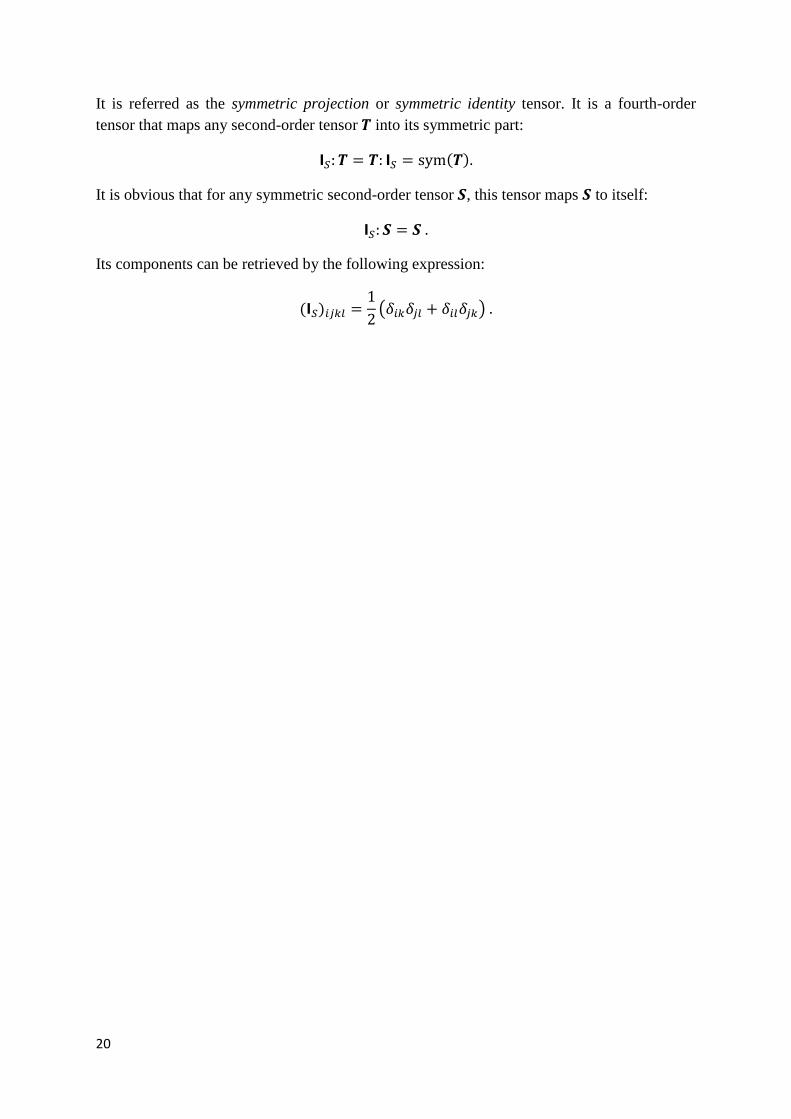
It is referred as the symmetric projection or symmetric identity tensor. It is a fourth-order

tensor that maps any second-order tensor into its symmetric part:

( )

It is obvious that for any symmetric second-order tensor , this tensor maps to itself:

Its components can be retrieved by the following expression:

( )

( )

21

Chapter 2: Theory of Rate-Independent Plasticity – Classical Yield

Criteria

The Mathematical Theory of Plasticity

The term inelasticity, is used to describe any constitutive behaviour other than elastic.

Generally, the inelastic behaviour includes viscoelastic, viscoplastic and elastoplastic

behaviour.

Throughout this thesis, only the elastoplastic behaviour is studied. In particular the theory of

plasticity is concerned with solids which when subjected to a loading program, may sustain

permanent deformations when completely unloaded. The assumption that these permanent

(plastic) deformations do not depend on the rate of the application of loads, leads to the

theory of rate-independent plasticity. The materials that can be adequately described by this

theory are called plastic or rate-independent plastic.

The adjective “plastic” comes from the Greek work “πλάσσειν”, meaning “to shape”. A large

number of engineering materials such as metals, soils, rocks can be modeled as plastic in a

wide range of applications. This is true despite the materials’ different nature and

constitution.

In this chapter, the mathematical theory of rate-independent plasticity is introduced. Plasticity

theory is a very large topic and clearly cannot be covered in a single chapter of a master

thesis. Thus, this brief review is restricted to infinitesimal deformations and aims to provide a

solid basis for the numerical simulation of elastoplastic solids.

2.1. Phenomenological Aspects

As already mentioned, in spite of their qualitatively distinct mechanical characteristics,

materials as contrasting as metals and soils share some common features of their

phenomenological behaviour that make them amenable to modeling by means of the theory

of plasticity. To illustrate all those common features, we begin by discussing a uniaxial

tension experiment of a metallic bar. The uniaxial tension test although it may appear simple,

it introduces some very important aspects of the plasticity theory.

“Of all mechanical tests for structural materials, the tension test is the most common. This is

true primarily because it is a relatively rapid test and requires simple apparatus. It is not as

simple to interpret the data it gives, however, as might appear at first sight.” J.J Gilman

[1969].

The immediate result of a tension test is a relation between the axial force and either the

change in length (elongation) of a gage portion of the specimen or a representative value of

longitudinal strain as measured by one or more strain gages. This relation is usually changed

to one between the stress (force F divided by cross-sectional area) and the strain (elongation

divided by gage length or strain-gage output) and is plotted as the stress-strain diagram.

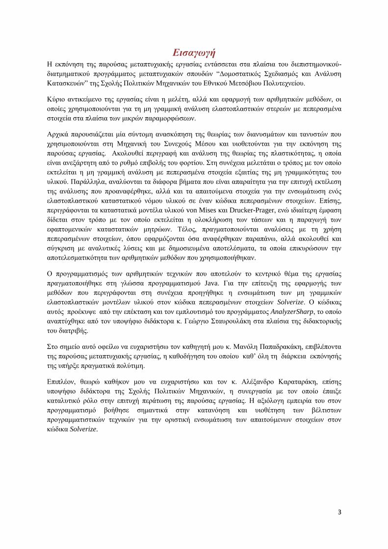
Uniaxial tension tests of ductile metals, produce stress-strain curves of the type illustrated in

the following figure.

22

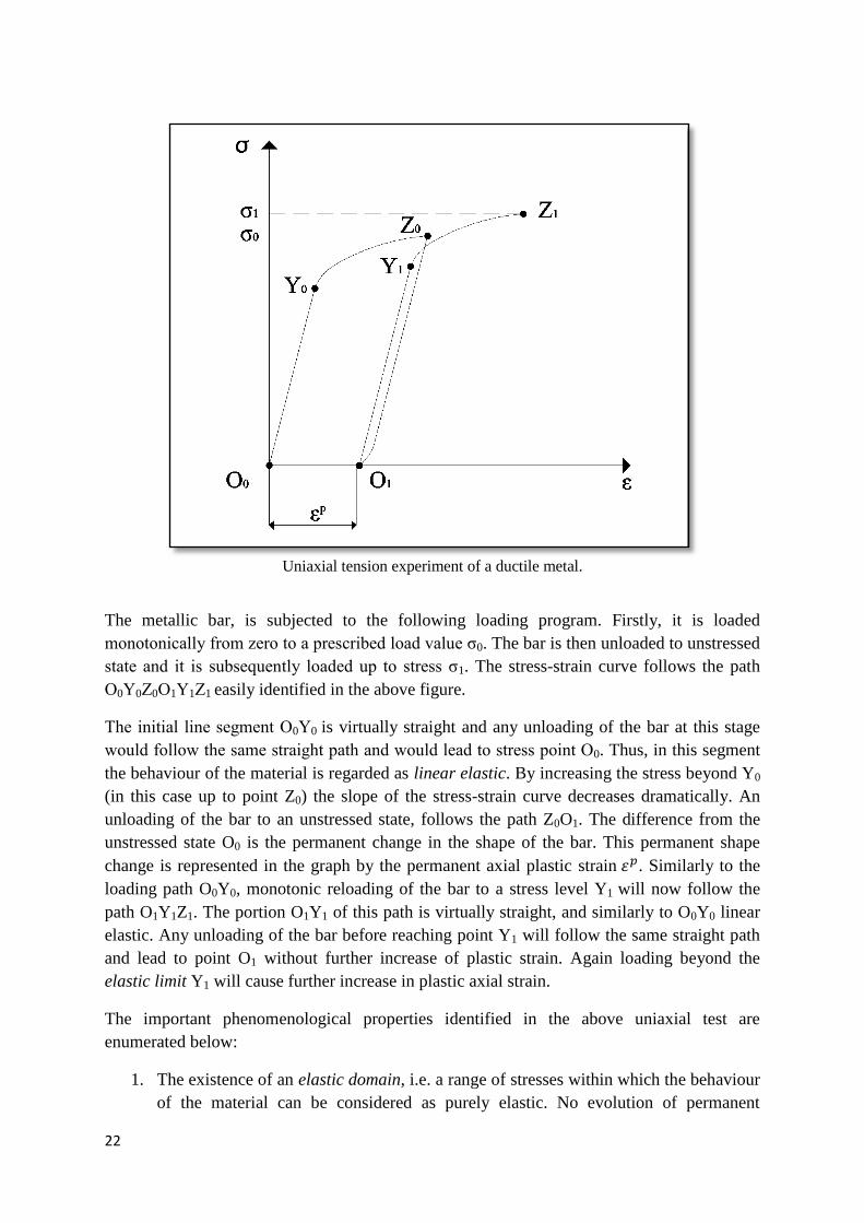
Uniaxial tension experiment of a ductile metal.

The metallic bar, is subjected to the following loading program. Firstly, it is loaded

monotonically from zero to a prescribed load value σ0. The bar is then unloaded to unstressed

state and it is subsequently loaded up to stress σ1. The stress-strain curve follows the path

Ο0Υ0Ζ0Ο1Υ1Ζ1 easily identified in the above figure.

The initial line segment Ο0Υ0 is virtually straight and any unloading of the bar at this stage

would follow the same straight path and would lead to stress point Ο0. Thus, in this segment

the behaviour of the material is regarded as linear elastic. By increasing the stress beyond Y0

(in this case up to point Z0) the slope of the stress-strain curve decreases dramatically. An

unloading of the bar to an unstressed state, follows the path Z0O1. The difference from the

unstressed state O0 is the permanent change in the shape of the bar. This permanent shape

change is represented in the graph by the permanent axial plastic strain . Similarly to the

loading path O0Y0, monotonic reloading of the bar to a stress level Y1 will now follow the

path O1Y1Z1. The portion O1Y1 of this path is virtually straight, and similarly to O0Y0 linear

elastic. Any unloading of the bar before reaching point Y1 will follow the same straight path

and lead to point O1 without further increase of plastic strain. Again loading beyond the

elastic limit Y1 will cause further increase in plastic axial strain.

The important phenomenological properties identified in the above uniaxial test are

enumerated below:

1. The existence of an elastic domain, i.e. a range of stresses within which the behaviour

of the material can be considered as purely elastic. No evolution of permanent

23

deformation (axial strain in this case) is possible when the material is subjected to

stresses lying within the elastic domain. This domain is delimited by the so-called

yield stress which in the uniaxial experiment, correspond to points Y0 and Y1 for

segments O0Y0 and O1Y1 respectively.

2. If the material is further loaded at the yield stress, then plastic yielding also denoted as

plastic flow takes place which leads to evolution of plastic strains.

3. The evolution of plastic strain during plastic flow is accompanied by the evolution of

the yield stress as well. This phenomenon known as hardening, can be identified by

the different yield stresses corresponding to points Y0 and Y1 of the stress-strain

curve.

It is emphasized that the properties identified above, can be observed not only in metals but

also in a wide variety of materials such as concrete, rocks, soils and many others. The

underlying mechanisms that give rise to these phenomenological characteristics can be

completely distinct and different for each type of material. It is also crucial to understand that

materials such as soils need other experimental procedures in order to verify their distinct

properties. A typical example is the triaxial shear test which is widely used when dealing

with materials such as soils which typically cannot resist tensile stresses.

The object of plasticity theory is to provide continuum constitutive models capable of

describe this kind of phenomenological behaviour for a variety of different materials that

possess the characteristics described and identified in the uniaxial tension test.

2.2. One-dimensional Constitutive Model

A simple mathematical model of the uniaxial tension experiment studied in the previous

section is formulated in what follows. As mentioned previously, the uniaxial experiment,

despite its simplicity, contains all the essential features that form the basis of the

mathematical theory of plasticity.

The uniaxial stress-strain curve illustrated in the previous section is approximated by an

idealized version shown in a following figure. The assumptions involved in the

approximation, are summarized as follows:

1. The difference between unloading and reloading curves (segments Z0O1 and O1Y1

respectively in the stress-strain curve of the uniaxial experiment) is ignored and points

Z0 and Y1, which correspond to the beginning of unloading and the beginning of the

plastic yielding of subsequent reloading coincide.

2. The transition between the elastic region and the elastoplastic region is now clearly

marked by a non-smooth change of slope (points Y0 and Y1).

24

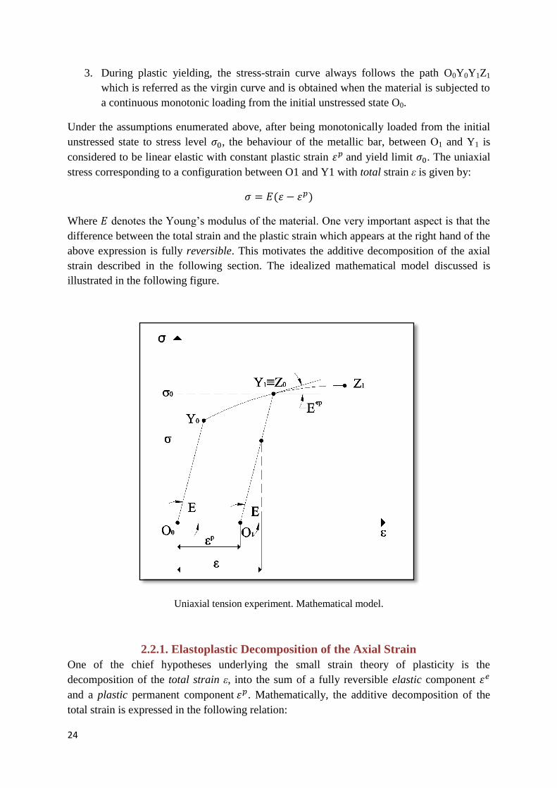
3. During plastic yielding, the stress-strain curve always follows the path O0Y0Y1Z1

which is referred as the virgin curve and is obtained when the material is subjected to

a continuous monotonic loading from the initial unstressed state O0.

Under the assumptions enumerated above, after being monotonically loaded from the initial

unstressed state to stress level , the behaviour of the metallic bar, between Ο1 and Y1 is

considered to be linear elastic with constant plastic strain and yield limit . The uniaxial

stress corresponding to a configuration between O1 and Y1 with total strain ε is given by:

( )

Where denotes the Young’s modulus of the material. One very important aspect is that the

difference between the total strain and the plastic strain which appears at the right hand of the

above expression is fully reversible. This motivates the additive decomposition of the axial

strain described in the following section. The idealized mathematical model discussed is

illustrated in the following figure.

Uniaxial tension experiment. Mathematical model.

2.2.1. Elastoplastic Decomposition of the Axial Strain

One of the chief hypotheses underlying the small strain theory of plasticity is the

decomposition of the total strain ε, into the sum of a fully reversible elastic component

and a plastic permanent component . Mathematically, the additive decomposition of the

total strain is expressed in the following relation:

25

where the elastic component is defined as:

2.2.2. The Elastic Uniaxial Constitutive Law

The definition of the elastic axial strain was given above. The constitutive law which relates

the elastic axial strain with the axial stress can be expresses as:

The next step in the definition of the axial constitutive law is to derive formulae that express

mathematically the three phenomenological aspects which were enumerated for the one-

dimensional constitutive model. A yield criterion as well as a plastic flow rule must be

formulated, combined with a hardening law which describes the evolution of the yield limit.

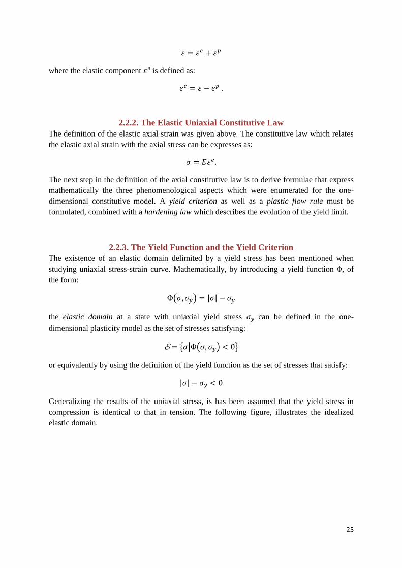
2.2.3. The Yield Function and the Yield Criterion

The existence of an elastic domain delimited by a yield stress has been mentioned when

studying uniaxial stress-strain curve. Mathematically, by introducing a yield function , of

the form:

( ) | |

the elastic domain at a state with uniaxial yield stress can be defined in the one-

dimensional plasticity model as the set of stresses satisfying:

{ | ( ) }

or equivalently by using the definition of the yield function as the set of stresses that satisfy:

| |

Generalizing the results of the uniaxial stress, is has been assumed that the yield stress in

compression is identical to that in tension. The following figure, illustrates the idealized

elastic domain.

26

Idealized elastic domain for the uniaxial model.

It should be noted that, at any stage, no stress level is allowed to exceed the current yield

stress. The so-called plastically admissible stresses lie either within the elastic domain or on

its boundary (the yield limit). In yield function terms, any plastically admissible stress must

satisfy:

( )

For stresses within the elastic domain, only elastic straining may occur whereas on its

boundary, either plastic yielding (plastic loading) or elastic unloading takes place. This yield

criterion can be expressed in terms of yield function and plastic strain rate (denoted by a dot

above the strain symbol):

( )

( ) {

2.2.4. The Plastic Flow Rule. Loading/Unloading Conditions

The above expressions define a criterion for plastic yielding. Upon plastic loading, the plastic

strain rate is positive under tension and negative under compression. Thus the plastic flow

rule can be mathematically established as:

( )

27

where sign is the signum function defined as:

( ) {

for any scalar and the other scalar is the plastic multiplier. The plastic multiplier is non-

negative:

and satisfies the complementarity condition:

All the above constitutive equations imply that the plastic strain rate vanishes within the

elastic domain:

and plastic flow occurs only when the stress level coincides with the elastic domain boundary

i.e. the current yield stress:

| | σ

Summarizing, the set of the following constraints, define the so-called loading/unloading

conditions of the elastoplastic model and establish when plastic flow may occur:

2.2.5. The Hardening Law

In order to completely characterize the uniaxial model, an additional component must be

introduced. By observing the uniaxial experiment, an evolution of the yield stress during

plastic yielding can be easily identified. This phenomenon is known as hardening. The

corresponding hardening law describes the relation between the evolution of the yield stress

and the accompanying plastic strain. The hardening phenomenon can be easily incorporated

to the uniaxial model by assuming that the yield stress is a given function:

( )

Where is the accumulated plastic strain. It is defined as:

∫ | |

The absolute value, ensure that both tensile and compressive plastic strains contribute to the

accumulated plastic strain. The curve defined by the hardening function introduced above is

usually referred as the hardening curve and it’s illustrated in the following figure.

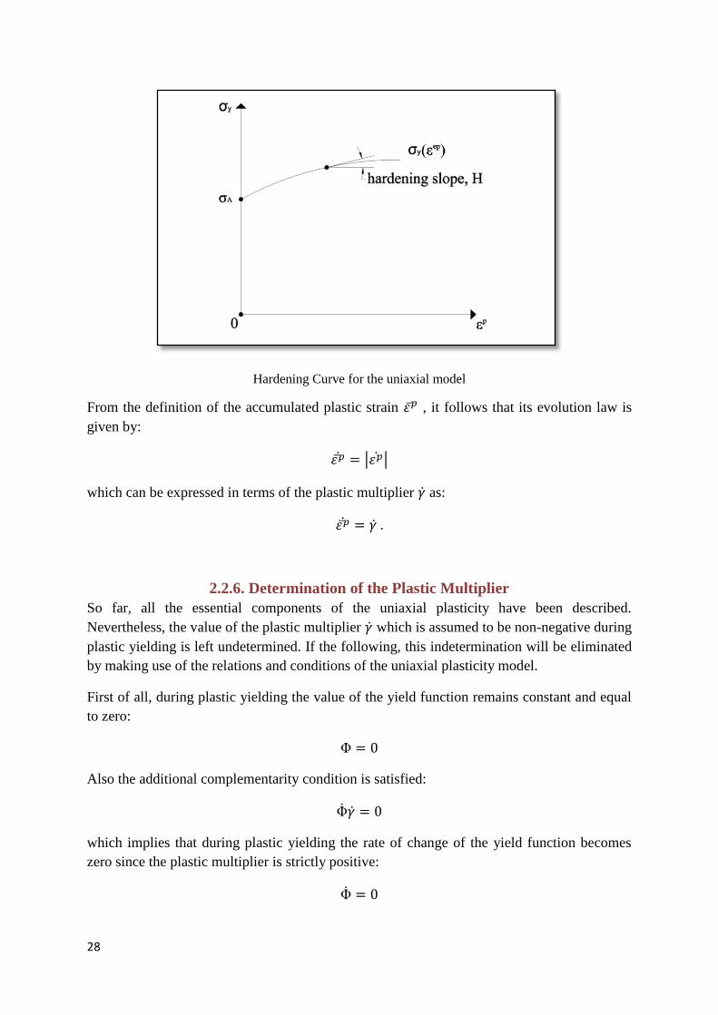
28

Hardening Curve for the uniaxial model

From the definition of the accumulated plastic strain , it follows that its evolution law is

given by:

| |

which can be expressed in terms of the plastic multiplier as:

2.2.6. Determination of the Plastic Multiplier

So far, all the essential components of the uniaxial plasticity have been described.

Nevertheless, the value of the plastic multiplier which is assumed to be non-negative during

plastic yielding is left undetermined. If the following, this indetermination will be eliminated

by making use of the relations and conditions of the uniaxial plasticity model.

First of all, during plastic yielding the value of the yield function remains constant and equal

to zero:

Also the additional complementarity condition is satisfied:

which implies that during plastic yielding the rate of change of the yield function becomes

zero since the plastic multiplier is strictly positive:

29

while the rate can take any value during elastic straining. The above condition, is called

the consistency condition. Now, by taking the time derivative of the yield function, we obtain

the following relation:

( ) | | ( )

where is the hardening modulus or hardening slope. The hardening modulus is tangent to

the hardening curve and is defined as:

As mentioned earlier, during plastic yielding, the rate of the yield function vanishes, so:

( )

From the elastic law and the decomposition of the strain, it follows:

( )

Finally, by combining the two previous relations, the plastic multiplier can be uniquely

determined:

( )

| |

2.2.7. The Elastoplastic Tangent Modulus

The final crucial component of the uniaxial model is the tangent relation between strain and

stress during plastic flow at a generic yield limit. This relation, can be established by making

use of the elastoplacstic tangent modulus as follows:

The elastoplastic tangent modulus can be calculated by the following relation which is

obtained by combining the flow rule, the above relation and the elastic law:

The hardening modulus can be expressed by the above relation as:

30

2.3. General Elastoplastic Constitutive Model

In the previous section the mathematical model of a uniaxial experiment with a ductile metal

has been presented and analyzed. This model contains all the essential components needed to

describe a general elastoplastic constitutive model. In this section, the generalization of the

concepts of the theory of plasticity will be described for two- and three-dimensional cases.

2.3.1. Additive Decomposition of the Strain Tensor

In the uniaxial case we have seen that axial strain can be decomposed into two parts i.e the

elastic and the plastic components. This holds for the multidimensional case as well but now

the corresponding decomposition is obtained by splitting the strain tensor into the sum of

an elastic component and a plastic component . That is:

The above tensors are known as the elastic strain tensor and the plastic strain tensor

respectively and the above relation can be written in rate form:

2.3.2. The Free Energy Potential and the Elastic Law

The starting assumption for the plasticity theory treated in this thesis, is that the free energy,

, is a function:

( )

of the total strain tensor, the plastic strain tensor which is considered as an internal variable

and a set of internal variables, associated with the phenomenon of hardening. By taking

into account the additive decomposition of the stain tensor, the free energy can be split as:

( ) ( ) ( )

( ) ( )

which is the sum of an elastic contribution, , which depends only one the elastic strain and

a contribution due to hardening, .

Now the Clausius-Duhem inequality reads:

(

)

where

31

is the hardening thermodynamical force and the symbol indicates the appropriate product

between and . The above inequality implies a general elastic law of the form:

so the requirements for non-negative dissipation can be reduced to:

( )

where is called the plastic dissipation function and it is defined by:

( )

In this thesis, the elastic behaviour of the materials treated is assumed to be linear and

isotropic. In this case, the elastic contribution to the free energy is given by the following

relation:

( )

( )

As a result, the elastic law between the elastic strain tensor and the corresponding stress

tensor can be described via the following relation:

where and are the shear and bulk moduli. The tensor is the deviatoric component of

the elastic strain tensor and the scalar ( ) is the volumetric elastic strain. Finally

is the standard fourth-order isotropic elasticity tensor which has the general format:

(

)

where for three-dimensional, plane strain and axisymmetric analyses, whereas in plane

stress:

32

2.3.3. Yield Criterion and Yield Surface

In the uniaxial yield criterion discussed previously in this section, it is clear that plastic flow

may occur when the uniaxial stress reaches a critical value, the uniaxial yield stress. This

principle was expressed by the use of a yield function whose value is negative when the stress

lies in the elastic region and becomes zero during plastic flow. This concept of yield function

can be extended for two and three-dimensional cases. The scalar yield function is now a

function of the stress tensor σ and a set A of hardening thermodynamical forces. Analogously

to the uniaxial case the elastic domain is defined as the set satisfying:

{ | ( ) }

Plastic yielding is impossible when the stress tensor of the material is in the elastic domain.

Again, the set of plastically admissible stresses is a set that includes the stresses lying in the

elastic domain or on its boundary:

{ | ( ) }

The set of stresses which is termed as yield locus and for which plastic flow may occur is the

boundary of the elastic domain, where the value of the yield function becomes zero. This

yield locus can be represented by a hypersurface in the space of stresses which is known as

yield surface. The graphical representation of the yield surface is possible only in the

principal stress space.

2.3.4. Plastic Flow Rule and Hardening Law

The next step for a characterization of a plasticity model requires the definition of the

evolution laws for the internal variables which are associated with the dissipative phenomena.

In this case, the internal variables consist of the plastic strain tensor and the set of

hardening variables. The following plastic flow rule and hardening law are then postulated:

where the tensor:

( )

is termed the flow vector in plasticity and the function:

( )

is the generalized hardening modulus which is the generalization of the hardening modulus

defined in the uniaxial case. It defines the evolution of the hardening variables.

Finally, the loading/unloading conditions defined for the uniaxial model hold in the general

case as well:

33

and define when evolution of plastic strains and internal variables may occur.

2.3.5. Flow Rules Defined from a Flow Potential

In multidimensional plasticity models, it is convenient to define the flow rule in terms of a

flow potential (the term plastic potential is also used). This approach begins by postulating a

flow potential with general form:

( )

from which the flow vector N can be obtained by differentiation by:

If the hardening rule is assumed to be derived from the same potential, then we have in

addition:

The plastic potential, is required to be a non-negative convex function of both and which

is zero-valued at the origin:

( )

In many plasticity models, the yield function can be used itself as a flow potential:

Such models are called associative or associated plasticity models. When this is not the case

the models are called non-associative. In this thesis, only associative plasticity models are

studied.

2.3.6. The Plastic Multiplier

As in the uniaxial case the procedure for determination of the plastic multiplier begins by

taking into consideration the complementarity condition:

which implies the consistency condition:

during plastic yielding. By differentiating the yield function with respect to time, the

following expression can be obtained:

34

Now by taking into account the additive decomposition of the strain tensor, the elastic law

and the flow rule, we substitute into the above expression and we obtain:

( ) ( )

By using the definition of the hardening thermodynamical force in terms of the free energy

potential which was derived in an earlier section and also by taking into consideration the

evolution law:

the rate of the yield function can be written in the form:

( )

( )

From the above and the consistency conditions which says that the rate of the yield function

during plastic yielding becomes zero, the plastic multiplier can be obtained by the

following formula:

( )

2.3.7. Rate Form and the Elastoplastic Tangent Operator

In the elastic region, the rate constitutive equation reads:

while during plastic flow the corresponding equation reads:

where is the elastoplastic tangent modulus given by:

( ) (

)

The elastoplastic tangent modulus is a fourth-order tensor and it is the multidimensional

equivalent of the elastoplastic scalar modulus introduced for the uniaxial model.

35

If the flow rule is associative, then is symmetric, while form models with non-associative

plastic flow is generally unsymmetric.

2.4. Classical Yield Criteria

In this section, some of the most common yield criteria used in engineering applications are

described in detail. Namely the von Mises, Mohr-Coulomb and Drucker-Prager criteria are

examined. Their basic characteristics are presented and various representations of the

according yield functions are established. In addition, the graphical representation of each

criterion in three dimensional principal stress space is shown.

2.4.1. Von Mises Yield-Criterion

The von Mises yield criterion was proposed by von Mises (1913) in order to describe plastic

yielding in metals. One of its main advantages is the absence of singularities in the yield

function which when present as in the case of the Tresca yield criterion, cause problems when

analytical solutions to simple boundary problems are sought. In addition it offers a number of

attractive features with respect to numerical integration of rate equations. Finally the von

Mises criterion due to its lack of corners in its graphical representation allows the simple

calculation of the differentials of the yield and plastic potential functions required in order to

obtain the elastoplastic modulus.

According to the von Mises criterion, plastic yielding begins when the stress deviator

invariant reaches a critical value. The yield surface constitutes of an infinite circular cylinder

in principal stress space with the principal diagonal (hydrostatic axis) as center axis. It is

easily understood that only the deviatoric stress tensor takes part in the definition of the von

Mises criterion. The pressure component of the stress tensor does not influence the plastic

yielding and that’s the reason why this criterion is characterized as a pressure-independent.

Mathematically, the yield function can be expresses in a number of ways:

( ) √ ( ( ))

( ) ( )

In the above relation, is used to describe the yield function, is the uniaxial yield stress

and q is the so-called von Mises effective or equivalent stress. The von Mises effective stress

is calculated from the expression:

( ) √ ( ( ))

where denotes the stress deviator. In terms of principal deviatoric stresses , the above

relation can be written as:

36

( )

( )

Additionally, the yield function can be expressed in terms of a shear yield stress τy :

( ) √ ( ( ))

The shear yield stress and the uniaxial yield stress for the von Mises yield criterion are related

via the following relation:

√

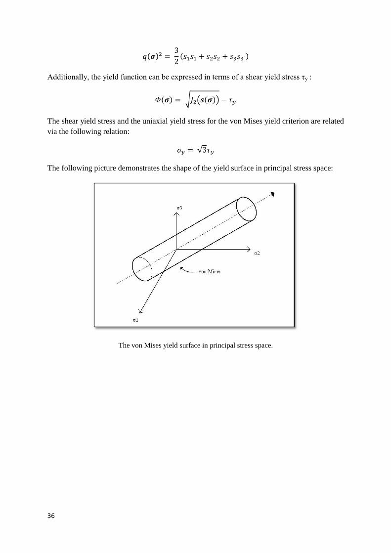
The following picture demonstrates the shape of the yield surface in principal stress space:

The von Mises yield surface in principal stress space.

37

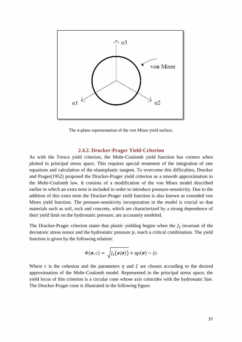
The π-plane representation of the von Mises yield surface.

2.4.2. Drucker-Prager Yield-Criterion

As with the Tresca yield criterion, the Mohr-Coulomb yield function has corners when

plotted in principal stress space. This requires special treatment of the integration of rate

equations and calculation of the elastoplastic tangent. To overcome this difficulties, Drucker

and Prager(1952) proposed the Drucker-Prager yield criterion as a smooth approximation to

the Mohr-Coulomb law. It consists of a modification of the von Mises model described

earlier in which an extra term is included in order to introduce pressure-sensitivity. Due to the

addition of this extra term the Drucker-Prager yield function is also known as extended von

Mises yield function. The pressure-sensitivity incorporation in the model is crucial so that

materials such as soil, rock and concrete, which are characterized by a strong dependence of

their yield limit on the hydrostatic pressure, are accurately modeled.

The Drucker-Prager criterion states that plastic yielding begins when the invariant of the

deviatoric stress tensor and the hydrostatic pressure , reach a critical combination. The yield

function is given by the following relation:

( ) √ ( ( )) ( )

Where c is the cohesion and the parameters and are chosen according to the desired

approximation of the Mohr-Coulomb model. Represented in the principal stress space, the

yield locus of this criterion is a circular cone whose axis coincides with the hydrostatic line.

The Drucker-Prager cone is illustrated in the following figure:

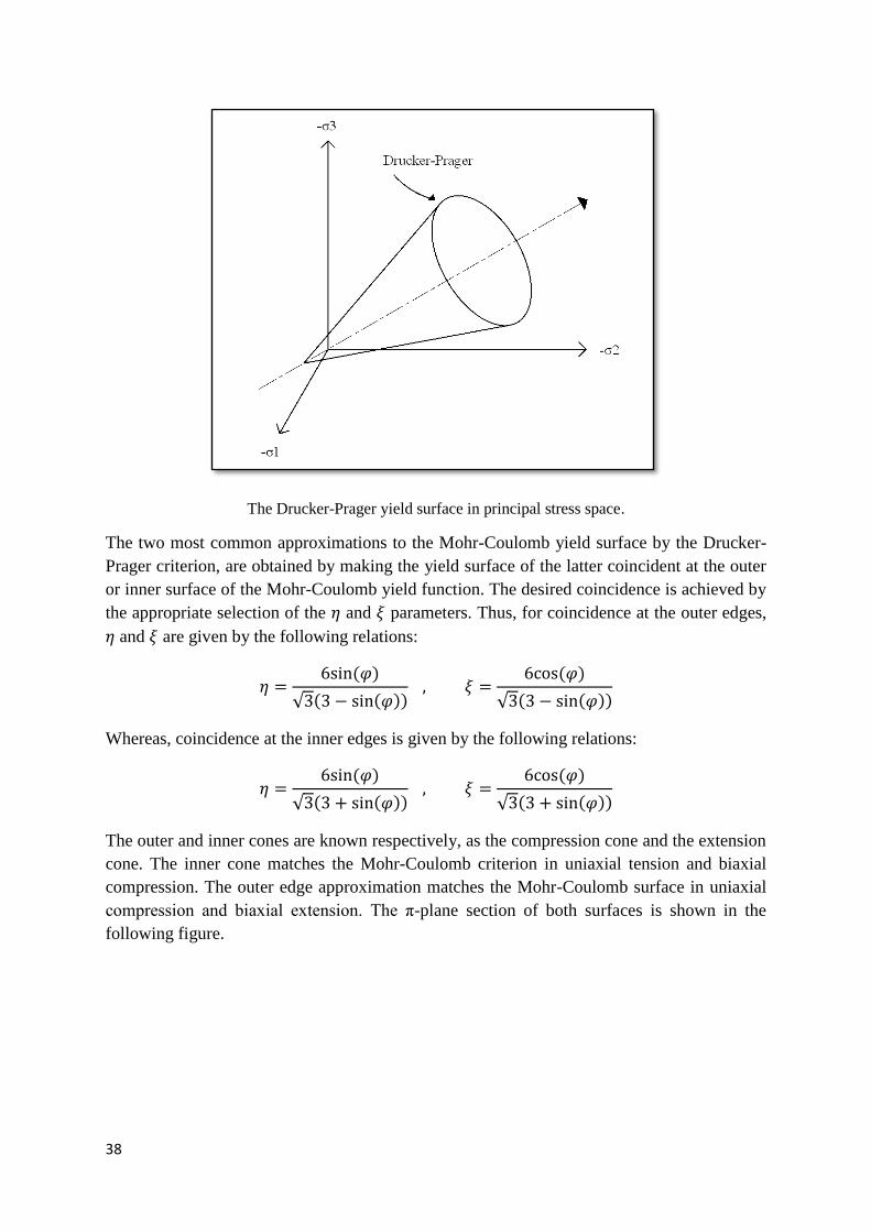
38

The Drucker-Prager yield surface in principal stress space.

The two most common approximations to the Mohr-Coulomb yield surface by the Drucker-

Prager criterion, are obtained by making the yield surface of the latter coincident at the outer

or inner surface of the Mohr-Coulomb yield function. The desired coincidence is achieved by

the appropriate selection of the and parameters. Thus, for coincidence at the outer edges,

and are given by the following relations:

( )

√ ( ( ))

( )

√ ( ( ))

Whereas, coincidence at the inner edges is given by the following relations:

( )

√ ( ( ))

( )

√ ( ( ))

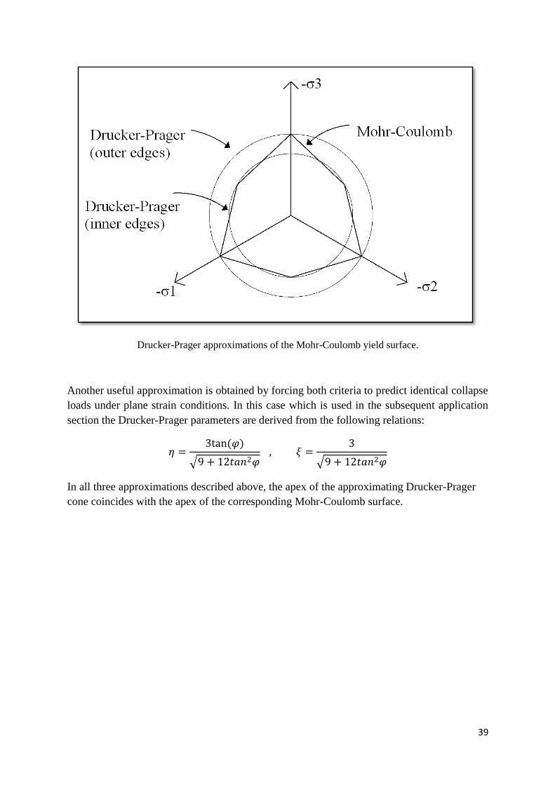
The outer and inner cones are known respectively, as the compression cone and the extension

cone. The inner cone matches the Mohr-Coulomb criterion in uniaxial tension and biaxial

compression. The outer edge approximation matches the Mohr-Coulomb surface in uniaxial

compression and biaxial extension. The π-plane section of both surfaces is shown in the

following figure.

39

Drucker-Prager approximations of the Mohr-Coulomb yield surface.

Another useful approximation is obtained by forcing both criteria to predict identical collapse

loads under plane strain conditions. In this case which is used in the subsequent application

section the Drucker-Prager parameters are derived from the following relations:

( )

√

√

In all three approximations described above, the apex of the approximating Drucker-Prager

cone coincides with the apex of the corresponding Mohr-Coulomb surface.

40

41

Chapter 3: Numerical Solution of the Elastoplastic Constitutive

Initial Value Problem with the Finite Element Method

3.1. The Incremental Finite Element Solution for Path-Dependent

Materials

When dealing with elastoplastic materials, the constitutive equations are path-dependent. This

means that the stress tensor cannot be calculated from the instantaneous value of the

infinitesimal strain tensor only. The whole history of strains to which the solid of interest has

been subjected needs to be known. The stress tensor is the solution of the constitutive initial

value problem whose general form is the following:

Given the initial values of the internal variables ( ) and the history of the infinitesimal

strain tensor,

( ) [ ]

find the functions ( ) and ( ) , for the stress tensor and the set of internal variables, such

that the constitutive equations

( )

|

( ) ( ( ) ( ))

are satisfied for every [ ].

3.1.1. The Incremental Constitutive Function

For a generic path-dependent material model, the solution of the above constitutive initial

value problem for a given set of initial conditions is usually not known for complex strain

paths ( ). Therefore, the use of an appropriate numerical algorithm for integration of the

rate constitutive equations is an essential requirement in the finite element simulations of

models including path-dependent materials. The choice of the particular integration technique

depends on the characteristics and of each specific material model. In general, some kind of

time or pseudo-time discretization is adopted along with some hypothesis on the deformation

path between adjacent time stations. Within the context of purely mechanical theory,

considering the time increment [ ] and by having the set of internal variables at

time , then the strain tensor at time must uniquely determine the strain tensor

through the integration algorithm. An approximate incremental constitutive function

for the stress tensor is defined:

( )

42

whose outcome , is expected to converge to the actual solution of the evolution problem

as the strain increments are reduced.

The numerical constitutive law is generally nonlinear and is path-dependent within one

increment. Within each increment is a function of alone. The integration algorithm

also defines a similar incremental constitutive function for the internal variables of the model:

( )

In the context of elastoplasticity the procedure of elastic predictor/return-mapping algorithms

is the numerical integration scheme which is going to be used in this thesis.

3.1.2. The Incremental Boundary Value Problem

Having defined the generic incremental constitutive law in the previous section, we can now

state the incremental or time-discrete version of the initial boundary problem:

Given the set of the internal variables at time , find a displacement field

such that

∫[ ( )

]

∫

for any , where and are the body forces and surface traction fields

prescribed at time . The set is defined as:

{ | }

where are the prescribed boundary displacements at .

3.1.3. The Nonlinear Incremental Finite Element Equation

After the standard finite element discretization of the incremental boundary value problem

introduced in the previous section, the problem is reduced to the following.

Find the nodal displacement vector at time such that the incremental finite element

equilibrium equation

( ) ( )

is satisfied, where ( ) and are assembled from the element vectors

( ) ∫

( ) ( ( ))

( ) ∫

( ) ∫

( )

43

The equilibrium equation is generally nonlinear. The source of nonlinearity is the

nonlinearity of the incremental constitutive function that takes part in the definition of the

element internal force vector.

In our case the use of proportional loading is used in the incremental finite element scheme.

Proportional loading is characterized by body force and surface traction fields given at an

arbitrary time instant , by:

where is the prescribed load factor at and , are prescribed, constant in time

fields. In this case, the global external force vector reduces to

where is computed only once at the beginning of the incremental procedure as the

assembly of element vectors

( ) ∫

( ) ∫

( )

3.1.4. Nonlinear Solution. The Newton-Raphson Scheme

The Newton-Raphson algorithm is particularly attractive for the solution of the nonlinear

incremental equilibrium equation. Due to the quadratic rates of asymptotic convergence it

offers, the Newton-Raphson method produces relatively robust and efficient incremental

nonlinear finite element schemes and is adopted in our case.

Each iteration of the Newton-Raphson scheme, comprises the solution of the linearized

version of the discretized incremental equilibrium equation.

At a state defined by the global displacement vector ( )

, the typical iteration ( ) of the

Newton-Raphson scheme, consists of solving the linear system of equations

( ) ( )

for ( ) , where we have defined the residual or out-of balance force vector

( ) ( ( ))

and is the global tangent stiffness matrix:

∫ ( )

| ( )

44

With the solution ( ) at hand, we apply the Newton correction to the global displacement

( ) ( ) ( )

or in terms of displacement increments,

( )

( )

where ( ) is the incremental displacement vector:

( ) ( ) ( )

The Newton-Rapshon iterations are repeated until after some iteration ( ), the following

convergence criterion is satisfied:

| ( )|

| |

where is a sufficiently small specified equilibrium convergence tolerance.The

corresponding displacement vector, ( )

, is then accepted as sufficiently small to the

solution of the incremental equilibrium equation:

( )

At the start of the Newton-Raphson iterations, we need an initial guess, ( )

. This initial

guess is usually taken as the converged equilibrium displacement vector of the previous

increment,

( ) or

( )

3.1.5. The Consistent Tangent Modulus

The global tangent stiffness is the assembly of the element tangent stiffness matrices:

( ) ∫

( )

where is the consistent tangent matrix – the matrix form of the fourth-order consistent

tangent operator

| ( )

This tensor possesses the symmetries:

45

The consistent tangent operator is the derivative of the incremental constitutive function .

This generally implicit function is typically defined by some numerical algorithm for

integration of the rate constitutive equations of the model. The derivation of this operator

consistent with the numerical integration used for the material model, is discussed thoroughly

in a following section in the context of elastoplasticity.

3.2. Preliminary Implementation Aspects for the Elastoplastic Constitutive Initial

Value Problem

The numerical procedure necessary for the implicit finite element solution of small strain

plasticity problems within the finite element framework presented in the previous sections

can be summarized into two most fundamental operations specific for every material model.

1. The state update procedure which, in the case of elastoplastic materials, requires the

formulation of a scheme for numerical integration of the rate elastoplastic evolution

equations. Within a pseudo-time increment [ ] , the state update procedure

gives the stresses and the internal variables at the end of the increment as a

function of the internal variables at the beginning of the increment and the strains

at the end of the increment:

( )

( )

The incremental constitutive functions and are defined by the integration

algorithm adopted and the stress delivered by is used to assemble the internal force

vector

∑

|

2. The computation of the associated consistent tangent modulus

to be used for the evaluation of a new tangent stiffness matrix whenever the Newton-

Raphson scheme requires for solution of the nonlinear finite element equilibrium

equations. The element tangent stiffness matrix is computed as

( ) ∑

46

3.2.1 The Elastoplastic Constitutive Initial Value Problem

Let us consider a point of a solid body with constitutive behaviour described by the

general elastoplastic model. Assume that at a given pseudo-time the elastic strain ( ),

the plastic strain tensor ( ) and all the elements of the set ( ) of hardening internal

variables are known at point . Furthermore, let the motion of be prescribed between

and a subsequent instant, . The prescribed motion, defines the history of the strain tensor,

( ), at the material point of interest between the time instants and . The basic

elastoplastic constitutive initial value problem at point is stated as follows.

Given the initial values ( ) and ( ) and the given history of the strain tensor, ( ),

[ ], find the functions ( ), ( ) and ( ) for the elastic strain tensor, hardening

internal variables set and plastic multiplier respectively that satisfy the reduced general

elastoplastic constitutive equations

( ) ( ) ( ) ( ( ) ( ))

( ) ( ) ( ( ) ( ))

( ) ( ( ) ( )) ( ) ( ( ) ( ))

for each instant [ ] , with

( )

| ( )

|

The above system of equation is reduced because the plastic flow equation has been

incorporated into the additive strain rate decomposition. Therefore the plastic strain tensor

does not appear explicitly in the above equations. The only unknowns are the elastic strain

tensor, the set of hardening variables and the plastic multiplier. With the solution ( ) at

hand, we can easily determine the history of the plastic strain tensor from the trivial relation

( ) ( ) ( )

As already mentioned, the solution of the above problem is generally unknown for complex

strain paths. Therefore the adoption of a numerical technique to find an approximate solution

becomes absolutely essential. A general framework for the above constitutive initial value

problem of elastoplasticity is described in the following section.

3.2.2. Euler Discretization: The Incremental Constitutive Problem

The starting point here is the adoption of an Euler scheme to discretize the equations of the

elastoplastic constitutive initial value problem. Here the backward or fully implicit Euler

scheme is chosen. Accordingly for integration within a generic pseudo-time interval

[ ], we replace all the rate quantities with corresponding incremental values within the

considered time interval and the functions , and with their values at the end of the time

47

interval, . The resulting discrete version of the elastoplastic constitutive problem is

states as follows.

Given the values and of the elastic strain tensor and the internal variables set at the

beginning of the pseudo-time interval [ ] and given the prescribed incremental strain

for this interval, solve the following system of algebraic equations

( )

( )

for the unknowns , and , subjected to the constraints

( ) ( )

where

|

|

In the above, we have adopted the notation

( ) ( ) ( )

with ( ) and ( ) denoting the value of ( ) respectively at times and . The

increment is called the incremental plastic multiplier. Once the solution has been

obtained, the plastic strain tensor at can be calculated as

so that all variables of the model are known at the end of the interval [ ] .

3.2.3. Solution of the incremental problem

Due to the presence of the complementarity condition

( ) ( )

the solution of the incremental elastoplastic problem presented in the previous section, does

not follow directly the conventional procedure for standard initial value problems. The

complementarity condition, gives rise to a two-step algorithm derived in the following.

First of all, it must be noted that the constraint , allows only for two mutually

exclusive possibilities enumerated below:

1. Null incremental plastic multiplier,

48

In this case there is no plastic flow or evolution of internal variables within the

considered time interval [ ] and the process is purely elastic. The third

constrain of the complementarity condition is automatically satisfied and ,

are given by:

In addition, the constraint

( )

must hold, where and are functions of and are defined through the

potential relations

|

|

2. Strictly positive plastic multiplier,

In this case, , and satisfy

( )

( )

and the second and third equations of the complementarity condition combined, result

in the constraint

( )

Finally the procedure which selects which one of the above cases holds and solves the

required equations is described in the next section.

3.2.4. The Elastic Predictor/Plastic Corrector Algorithm

The nature of the above problem motivates the establishment of a two-step algorithm in

which the two possible sets of equations are employed sequentially and the final solution is

selected as the only valid one. The strategy adopted is the following:

a) The Elastic Trial Step.

Firstly we assume that the null incremental plastic multiplier situation ( )

occurs. In other words, we assume that the step [ ] is purely elastic. This

49

solution which is not necessarily the actual solution of the problem is called the

elastic trial solution. According to the elastic trial solution:

The corresponding stress and hardening force are called the elastic trial stress and the

elastic trial hardening force and are given by the known potential relations:

|

|

The above variables are collectively called the elastic trial state. If the elastic trial

state is indeed the solution of the problem, then it must also satisfy the constraint:

(

)

which means that the elastic trial stress state, lies within the elastic domain or on its

boundary which is the yield surface. Therefore, if the constraint is satisfied the state

variables are updated as:

( ) ( )

and the algorithm is terminated. Otherwise the elastic trial state is not plastically

admissible and the solution must be obtained from the plastic corrector step described

next.

b) The Plastic Corrector Step or Return-Mapping Algorithm.

Since this step is applied only if the elastic trial step is not plastically admissible, the

only option left is to solve the system of algebraic equations:

( )

( )

( )

which are of course complemented with the potential relations

|

|

The solution of the above system must satisfy

50

51

Chapter 4:Numerical Implementation of Classical Elastoplastic

Models

4.1. The von Mises Plasticity Model

Firstly, the basic points of the implemented von Mises plasticity model are summarized

below. The model that we are going to analyze adopts the fully implicit algorithm and

comprises:

1. A linear elastic law

where is the standard isotropic elasticity tensor.

2. A yield function of the form

( ) √ ( ( ))

where

( )

is the uniaxial yield stress – a function of the accumulated plastic strain, .

3. A standard associative flow rule

with the (Prandtl-Reuss) flow vector, , explicitly given by

√

‖ ‖

4. An associative hardening rule, with the evolution for the hardening internal variable

given by

√

‖ ‖

52

4.1.1 The Implicit Elastic Predictor/Return Mapping Scheme

Given the strain increment

Δ

corresponding to a typical pseudo-time increment [ ] , and given the state variables

{ } at , the elastic trial strain and trial accumulated plastic strain are given by

Δ

The corresponding trial stress is computed as:

or, equivalently, by applying the hydrostatic/deviatoric decomposition

Where and , denote, respectively, the deviatoric and hydrostatic stresses, and are,

respectively, the shear and bulk moduli and the subscripts and in the elastic trial strain

denote, respectively, the deviatoric and volumetric components. The trial yield stress is

simply

(

)

Having computed the elastic trial state, the next step in the algorithm is to check whether

lies inside or outside of the trial yield surface:

If lies inside the yield surface, i.e. if

( )

then the process within the interval [ ] is purely elastic and the elastic trial

state itself is valid and itself is the solution to the integration problem. In this case,

is updated.

53

Otherwise, the process is elastoplastic within the interval [ ] and the return-

mapping procedure which is going to be described in the following section has to be

applied.

The fully implicit return-mapping equations for the von Mises model consists of the

following set of nonlinear equations:

Δ √

‖ ‖

Δ

√ ( ) ( )

which has to be solved for ,

and Δ and where

( ) [

]

After the solution of the above system, the plastic strain tensor can be updated according

to the following formula:

Δ √

‖ ‖

4.1.2. Single-equation return-mapping

The above system can be substantially simplified. In fact, it can be reduced to a single

nonlinear equation that has the incremental plastic multiplier Δ as the only unknown. For

this simplification to be achieved, it should be noted firstly that the von Mises flow vector is

purely deviatoric so that the deviatoric/volumetric split gives:

Δ √

‖ ‖

Equivalently, in stresses terms we have:

54

Δ √

‖ ‖

which means that the return-mapping affects only the deviatoric stress component. The

hydrostatic pressure , has its value computed at the predictor state and can, therefore, be

eliminated from the system of eqiuations. Rearranging of the deviatoric stress-update formula

gives:

( √

Δ

‖ ‖)

From the above relation, it becomes clear that the trial and the updated deviatoric stresses are

co-linear. This implies that

‖ ‖

‖ ‖

Substitution of the above identity into the deviatoric stress-update formula gives

( √

Δ

‖ ‖)

( Δ

)

where

√ (

)

is the elastic trial von Mises effective stress. It is important to note that as is a constant

tensor during the return-mapping procedure, the updated deviatoric stress tensor is a

linear function of Δ only. Also the fully implicit return-mapping derived above, implies that

the updated deviatoric stress tensor is obtained by scaling down the trial deviatoric stress by

the factor ( Δ ). Finally, substitution of the above relation in the plastic

consistency condition produces the generally nonlinear scalar equation, having Δ as the

only unknown:

(Δ ) Δ (

Δ )

55

With the solution of the above equation and Δ at hand, the state variables are updated as

follows:

( Δ

)

[ ]

Δ

4.1.3. Linear Isotropic Hardening and Perfect Plasticity: The Closed-Form

Return Mapping

It should be noted that the main source of nonlinearity in the von Mises return-mapping

equation is the hardening curve, defined by the given function ( ). For linear

hardening materials, this function is linear and is expressed as:

where is the initial yield stress and is the constant hardening modulus. In such cases, the

plastic consistency condition reads:

(Δ ) Δ [ (

Δ ) ]

and the incremental plastic multiplier can be obtained in closed form a

Δ

and the Newton-Raphson algorithm is not needed. In the case of perfect plasticity the

above expression reads:

Δ

In this case, the updated stress is simply the projection of the elastic trail stress onto the fixed

yield surface along its radial direction. It is the closest point projection of the trial stress onto

the yield surface. The return mapping for this case is illustrated in the following figure.

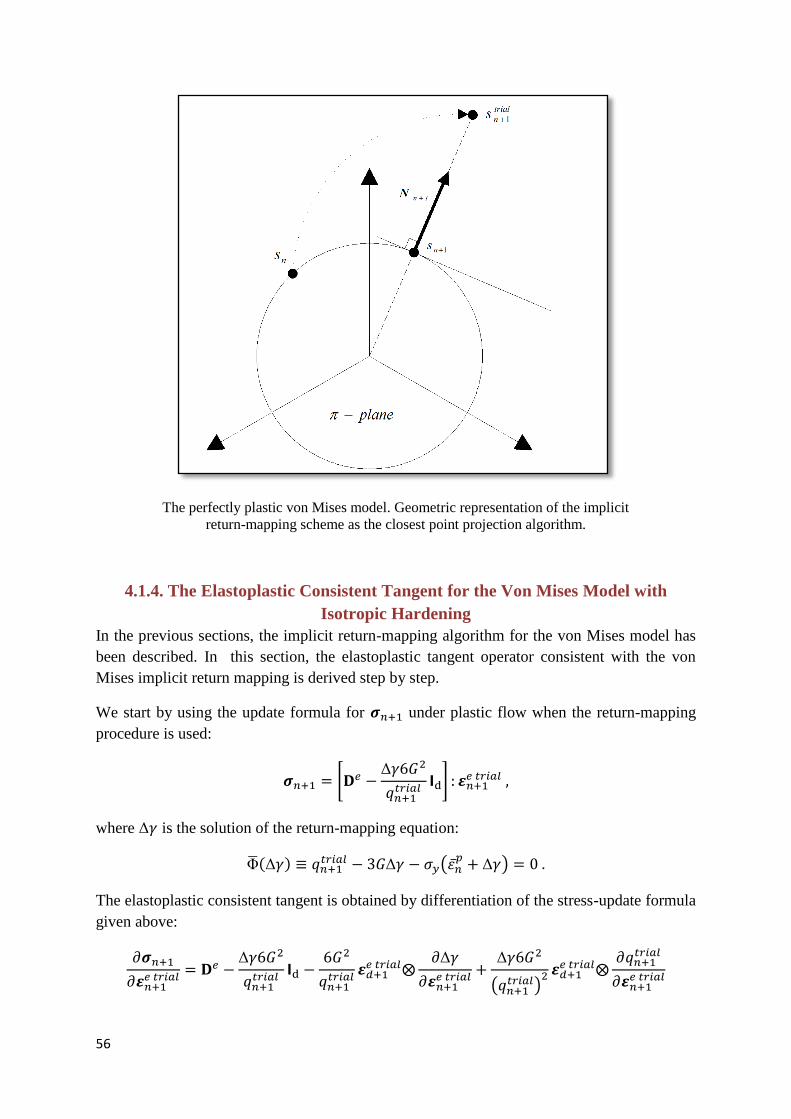
56

The perfectly plastic von Mises model. Geometric representation of the implicit

return-mapping scheme as the closest point projection algorithm.

4.1.4. The Elastoplastic Consistent Tangent for the Von Mises Model with

Isotropic Hardening

In the previous sections, the implicit return-mapping algorithm for the von Mises model has

been described. In this section, the elastoplastic tangent operator consistent with the von

Mises implicit return mapping is derived step by step.

We start by using the update formula for under plastic flow when the return-mapping

procedure is used:

[

Δ

]

where Δ is the solution of the return-mapping equation:

(Δ ) Δ (

Δ )

The elastoplastic consistent tangent is obtained by differentiation of the stress-update formula

given above:

Δ

Δ

Δ

( )

57

By the definition of and using some tensor calculus, we obtain:

√

where the unit flow vector is defined as:

√

‖ ‖

‖ ‖

In addition, the differentiation of the implicit return mapping equation gives:

Δ

√

where is the slope of the hardening curve:

| Δ

By combining all the above expressions, the following implicit expression for the

elastoplastic tangent operator consistent with the implicit return-mapping for the isotropically

hardening von Mises model is obtained:

Δ

(Δ

)

( Δ

)

(Δ

)

Finally, it should be noted that the operator in the present case and for this particular

model and numerical integration algorithm is symmetric.

58

4.2. The Drucker-Prager Model

In this section, we focus on the implementation of the Drucker-Prager model with isotropic

hardening

4.2.1. The Drucker-Prager constitutive equations

The Drucker-Prager yield surface is defined by means of the yield function:

( ) √ ( ( )) ( )

where:

( )

[ ]

In the above relations is the hydrostatic pressure and is the cohesion. The constants and

are calculated according to the required approximation to the Mohr-Coulomb criterion.

The general non-associative flow rule will be adopted but only the associative case will be

studied. The flow potential for the non-associative model is:

( ) √ ( ( )) ( )

where the constant depends on the dilatancy angle and is calculated according to the

required approximation to the Mohr-Coulomb law by replacing the frictional angle with

in the relations that give and where given in an earlier chapter. The flow rule reads:

where for the smooth portion of the yield surface, the flow vector is given by:

√ ( )

while at the cone apex the flow vector is a subgradient of .

A general associative isotropic strain hardening is adopted for the Drucker-Prager model. The

associative evolution equation for the accumulated plastic strain is:

while at the apex of the Drucker-Prager cone:

59

4.2.2. Integration Algorithm for the Drucker-Prager model

The Drucker-Prager material model has two main features. Firstly, only one singularity exists

on the yield surface, at the apex of the cone. Secondly, the Drucker-Prager yield surface as

well as the resulting flow vector field resulting from the generally non-associative flow

potential, are fully symmetric about the hydrostatic axis.

For materials with linear elastic law, the general return-mapping update formula for the stress

tensor is:

Δ

where Δ is the return vector. As a consequence of the symmetry about the

hydrostatic axis, whenever the above formula is applied, regardless of whether lies on

the smooth portion of the cone or on its apex, the return vector is always parallel to the plane

that contains and the hydrostatic axis. Thus the return-mapping algorithm can be

completely formulated in such a plane of stress space. Since the corresponding flow vector

differs for the smooth portion of the cone and its apex, two possible explicit forms exist

for the return-mapping algorithm. They are treated separately in the following section.

4.2.3. Return to the smooth portion of the cone

In a previous section, the flow vector for the smooth portion of the cone was defined by:

√ ( )

The corresponding increment of plastic strain reads:

Δ Δ Δ (

√ ( )

)

The corresponding stress-update formula is:

Δ [ ( ) ( ) ]

Δ (

√ ( )

)

Simplification of the above expression can be obtained by noting that, due to the definition of

, the following identity holds:

( )

( )

Substitution of the above identity into the stress-update formula, gives:

60

Δ

(

√ ( )

)

which can be equivalently written in terms of deviatoric and hydrostatic components:

(

Δ

√ ( ))

Δ

The consistency condition in the present case is given by:

( ) ( )

The updated accumulated plastic strain is obtained from:

Δ

with

Δ Δ

Finally, the substitution of the two above expressions in the consistency condition, results in

the following (generally nonlinear) equation for the incremental plastic multiplier Δ

(Δ ) √ ( ) Δ (

Δ ) ( Δ )

4.2.4. Return to the apex

At the apex, the return vector must be contained is the complementary cone of the yield

surface. The consistency condition in this case is reduced to:

( Δ )

Δ

By introducing the discretised form of the accumulated plastic strain the final return-mapping

equation for the Druckker-Prager apex is obtained:

(Δ ) (

Δ )

Δ

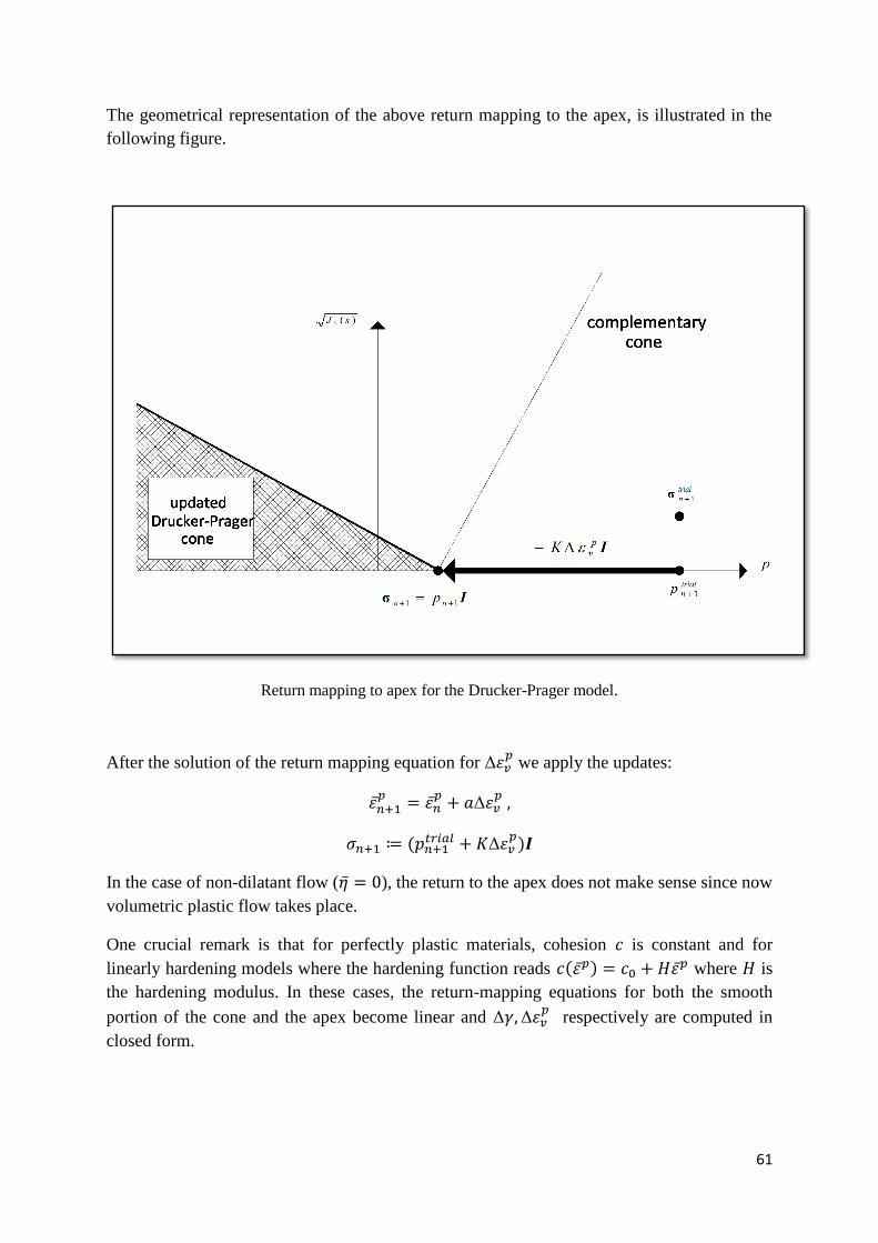
61

The geometrical representation of the above return mapping to the apex, is illustrated in the

following figure.

Return mapping to apex for the Drucker-Prager model.

After the solution of the return mapping equation for Δ we apply the updates:

Δ

( Δ

)

In the case of non-dilatant flow ( ), the return to the apex does not make sense since now

volumetric plastic flow takes place.

One crucial remark is that for perfectly plastic materials, cohesion is constant and for

linearly hardening models where the hardening function reads ( ) where is

the hardening modulus. In these cases, the return-mapping equations for both the smooth

portion of the cone and the apex become linear and Δ Δ respectively are computed in

closed form.

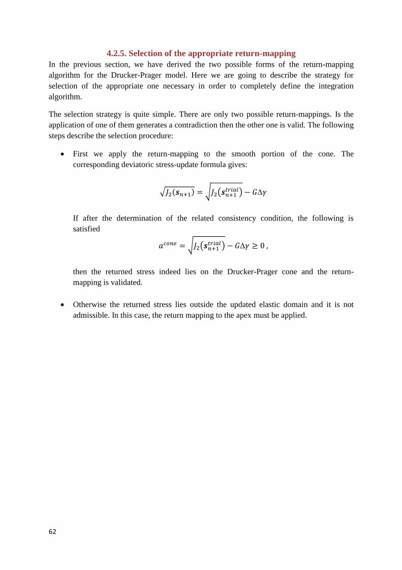
62

4.2.5. Selection of the appropriate return-mapping

In the previous section, we have derived the two possible forms of the return-mapping

algorithm for the Drucker-Prager model. Here we are going to describe the strategy for

selection of the appropriate one necessary in order to completely define the integration

algorithm.

The selection strategy is quite simple. There are only two possible return-mappings. Is the

application of one of them generates a contradiction then the other one is valid. The following

steps describe the selection procedure:

First we apply the return-mapping to the smooth portion of the cone. The

corresponding deviatoric stress-update formula gives:

√ ( ) √ ( ) Δ

If after the determination of the related consistency condition, the following is

satisfied

√ ( ) Δ

then the returned stress indeed lies on the Drucker-Prager cone and the return-

mapping is validated.

Otherwise the returned stress lies outside the updated elastic domain and it is not

admissible. In this case, the return mapping to the apex must be applied.

63

The following figure illustrates the above procedure

Selection of the appropriate return-mapping for the Drucker-Prager model.

4.2.6. Consistent Tangent Operator for the Drucker-Prager Model

The final step for the Drucker-Prager model, is the calculation of the elastoplastic tangent

associated with the integration algorithm described in the previous sections. The difference

between the Drucker-Prager model and the von Mises model described earlier is that there are

two possible return-mapping schemes i.e. the return-mapping to the smooth portion of cone

and the return-mapping to the apex. As a result two explicit forms of the elastoplastic tangent

exist. The actual elastoplastic tangent chosen in order to assemble the tangent stiffness matrix

is the one consistent with the last application of the return-mapping procedure at each Gauss

point.

64

4.2.6.1. Tangent consistent with the smooth portion return

Firstly, we have the deviatoric stress-update formula of the return-mapping to the smooth part

of the cone:

( Δ

√ ( )) (

Δ

√ ‖ ‖

)

By differentiating the above expression:

[( Δ

√ ‖ ‖

)

Δ

√ ‖ ‖

√ Δ ]

where the second-order tensor is the unit tensor parallel to :

‖ ‖

Next we have the update formula form the hydrostatic pressure:

Δ (

Δ )

Differentiation gives:

( Δ )

Now by linearizing the consistency conditions and using the elastic relation, we can obtain

the expression relating Δ and the differentials of trial strains:

√

( ) Δ

which results in the identity:

Δ

(√

)

Finally by substitution of the above relation to the differentiated version of the stress-update

expression, and by using the identity:

the explicit expression for the elastoplastic tangent consistent with the one-vector return is

obtained after some manipulation as:

( Δ

√ ‖ ‖

) (Δ

√ ‖ ‖

)

√ ( ) ( )

65

where is the deviatoric projection vector and is defined as:

4.2.6.2. Tangent consistent with the return-mapping to the apex

The key point in this case is that the stress deviator vanishes. The differential of the

updated stress is simply:

The associated elastoplastic tangent modulus is given by:

Now, recalling the hydrostatic pressure update formula:

Δ

we can differentiate and obtain:

Δ

Differentiating the residual equation of the return-mapping to the apex it is possible to obtain

the explicit expression that gives Δ :

( ) Δ

Δ (

)

Finally, substituting the formula into the hydrostatic pressure update expression and also

making use of the elastoplastic tangent modulus identity we obtain the explicit expression for

the tangent operator consistent with the return to the apex return-mapping:

(

)

which vanishes if the hardening modulus .

66

4.3. The Plane Stress-Projected von Mises Model

First of all, it is convenient to explain the meaning of plane stress-projected models. A plane

stress-projected plasticity model, is defined by a set of evolution equations that:

Involve only in-plane stress and strain components

Are equivalent to the three-dimensional model with the added plane stress constraints

defined for plane stress-conditions.

As a result, the in-plane stress/strain components are the primary variables which are

determined by the solution of the rate evolution equations. The out of plain strain component

is a dependent variable and can be calculated as a function of the in-plane strain components.

In the situation of linear elasticity being studied, the plane stress-projected elastic constitutive

equation can be written in complete analogy to the plane stress linear elasticity. So we can

write the stress-strain relations in matrix-vector form as follows:

{

}

[

] {

}

The out-of-plane axial strain can be calculated by:

( )

Obviously plane stress conditions require:

The general three-dimensional von Mises model with isotropic hardening is defined by the

following set of equations rewritten for consistency:

√ ( ) ( )

√

‖ ‖

Whereas in plane stress conditions the following constraints are added:

67

( ) (

) ( ) (

) ( )

4.3.1 The plane stress-projected equations

In order to obtain the plane stress-projected von Mises equations, firstly we need to derive

explicit expressions which relate the dependent out-of-plane elastic and plastic strain

components to the in-plane components. We start by taking into considerations that, as the

elastic behaviour is linear and isotropic, the plane stress constraints for the out-of-stress

components are equivalent to:

(

)

In addition, the plastic incompressibility that follows from the flow rule, gives:

(

)

Moreover, as the out of plane components of the stress deviator vanish under plane stress

conditions, it also follows from the flow rule that:

Summarizing, the history of the out-of-plane strain components is automatically prescribed

as:

( ) ( ) ( )

( )

( ) ( ) ( )

( )

( ) [

( ( )

( )) ( )

( )]

With the history of the out-of-plane strain components completely prescribed, we can now

eliminate them from the original set of equations of the general von Mises plasticity model.

This results in the plane stress-projected set of equations which, in component form, is given

by:

ε

√

( ) (

)

√

√ ( )

68

where denote the components of the plane stress elasticity tensor.

In order to derive the third and fourth equations above, we have made use of the identity:

‖ ‖ √

( )

which is obtained by introducing the plane stress constraints into the definition of the

deviatoric stress tensor and the Euclidean norm of a tensor:

[ ] ‖ ‖ √

4.3.2. Matrix Notation

A compact representation of tensor quantities involved in plane stress-projected equations for

the von Mises model can be obtained by making use of the following matrix and vector

notations:

[ ] [ ]

[ ] [

]

[

]

Also we introduce a special matrix denoted by which gives the deviatoric stress vector

when multiplied by the stress vector:

and it has the components:

[

]

With the above matrix/vector notation and by using matrix , the plane stress-projected

equations can be written in compact form:

69

√

(

)

√

√

where now, denotes the plane stress elasticity matrix. In the following section we are

deriving the integration algorithm. In order to accomplish it, the squared form of the yield

function will be introduced. The third, fourth and fifth equations above are written in squared

form:

( )

√

4.3.3. The Plane Stress-Projected Integration Algorithm

Within the framework of general elastic predictor/return-mapping schemes described in the

previous chapter and taking [ ] as the underlying pseudo-time interval, we start by

computing the predictor state:

Δ

ε ε

where Δ is the vector of in-plane incremental strains within the considered interval

[ ] :

Δ

The next step is to check for plastic admissibility of the elastic trial state. We then compute

the (using the squared form of the yield function):

( )

(ε )

70

If the trial state is admissible, i.e. if:

then the process is elastic within the time interval [ ] and we update:

( ) ( )

Otherwise, the return mapping algorithm must be applied and is described in the following

section.

4.3.4. The plane stress-projected return mapping

The implicit return mapping in the present case consists of solving the following system of

algebraic equations:

Δ

ε ε

Δ √

( )

( )

(ε )

for ε

and Δ where is a function of defined by the elastic law.

In complete analogy to the three-dimensional von Mises model, the number of unknowns of

the plane stress-projected return-mapping equations can be reduced. So the above set of

equations can be reduced to a single equation having the incremental plastic multiplier Δ as

the only unknown. This can be achieved by substituting the second equation to the third and

by rearranging the first equation, using the inverse of the elastic law:

[ Δ ]

( )

(ε

Δ √

( ) )

where the unknowns now are the stress vector, and the incremental plastic multiplier Δ

and is the inverse of the elastic matrix:

( )

Finally, by substituting the first equation to the second equations which represents the

consistency condition, the return-mapping for the plane stress-projected von Mises plasticity

model is reduced to the following scalar nonlinear equation having the incremental plastic

multiplier Δ as the only unknown:

71

(Δ )

(Δ )

(ε

Δ √

(Δ ))

In order to keep the notation as compact as possible, we have conveniently defined:

(Δ ) ( )

(Δ ) (Δ )

Where matrix (Δ ) is defined as:

(Δ ) [ Δ ]

Thus the return mapping is carried out as follows. Firstly we solve the consistency condition

using the Newton-Raphson algorithm. Then with the incremental plastic multiplier Δ

known, we update the other variables:

(Δ )

ε ε

Δ √

(Δ )

The in-plane plastic stresses can also be updated if necessary by:

Δ

One very crucial remark regarding the plane stress-projected return-mapping algorithm of the

von Mises plasticity model, is that is always nonlinear in Δ , regardless of the prescribed

function .This is in contrast with its three-dimensional counterpart whose main source of

nonlinearity is the hardening curve and which becomes linear for perfectly plastic and

linearly hardening models.

4.3.5. Newton-Raphson return-mapping solution

In the present case where the elastic behaviour is isotropic the explicit expression for the

solution of the consistency condition, as well as the calculation of matrix (Δ ) can be

significantly simplified. The key point is the fact that matrices and share the same

eigenvectors so that they both have a diagonal representation on the same basis. The same

fact holds for matrices and . So by applying the orthogonal transformation :

[

√

√

√

√

]

72

to and we obtain their diagonal representations:

[

]

[

]

On the same basis, the matrix (Δ ) has the diagonal representation:

(Δ ) [ Δ ]

[ ( )

( ) Δ

Δ

Δ ]

Where [ ] . The corresponding representation of the elastic trial stress vector is:

[

√ (

)

√ (

)

]

With all the transformed variables at hand, the expression that gives (Δ ) can be written in

the simpler form:

(Δ ) ( )

(Δ ) (Δ )

( )

( (Δ ))

(

)

[ Δ ( )

]

(

) (

)

( Δ )

Finally, using the orthogonal transformation we can calculate the matrix (Δ ) which takes

part in the stress update formula:

73

(Δ ) (Δ )

which leads to the explicit form:

(Δ )

[

(

)

(

)

(

)

(

)

]

with ,

, representing the diagonal terms of matrix (the diagonal representation

of which are given here for consistency:

( )

( ) Δ

Δ

4.3.6. The Elastoplastic Consistent Tangent Operator

With the matrix/vector notation adopter throughout the preceding derivations, the

elastoplastic tangent matrix is defined as:

The explicit expression for the elastoplastic tangent matrix is derived in the same way as its

three-dimensional counterpart. We start by combining the following equations:

[ ]

Beginning with the first equation:

[ ] [ ]

[ ]

[ ]

where the matrix is defined as:

[ ]

We continue by differentiating the derived equation:

[ ]

The plastic consistency condition is:

74

( )

( )

(

√

( ))

So by differentiating it we obtain the following:

√

( √

√ )

(

)

In the above, we have used the identity √

, which holds during plastic flow. From the

above equation, solving with respect to we have:

(

)

By making use of the elastic law, can now be defined in terms of matrix as:

( )

At this point, we can remind the useful relation which gives the differential of the inverse of a

matrix:

( )

for any invertible matrix .

By using the above relation, we can calculate the differential of the matrix :

[ ] ([ ] ) [ ] ( )[ ]

Direct differentiation of the expression between and the matrix , gives:

( )

( )

(

)

It has been proved that:

(

)

(

) (

)

75

Solving with respect to and substituting in the following:

[ ]

results to the following relation:

[ ( ) ( )]

where the scalar is defined as:

Finally we can write the explicit expression for the calculation of the elastoplastic consistent

tangent operator:

( ) ( )

The same procedure used to calculate matrix used for the update of the stress vector, can be

used in order to derive an explicit formula for matrix . So we arrive at the following:

( )

[

(

)

(

)

(

)

(

)

]

with:

( )

76

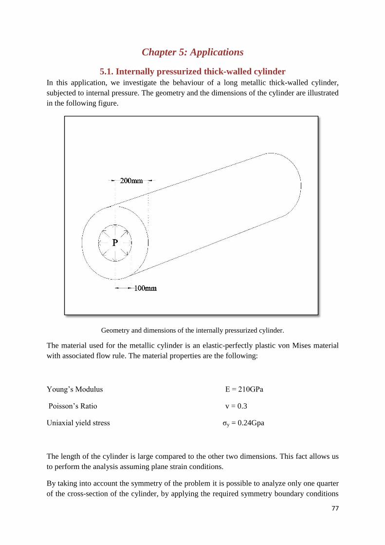
77

Chapter 5: Applications

5.1. Internally pressurized thick-walled cylinder

In this application, we investigate the behaviour of a long metallic thick-walled cylinder,

subjected to internal pressure. The geometry and the dimensions of the cylinder are illustrated

in the following figure.

Geometry and dimensions of the internally pressurized cylinder.

The material used for the metallic cylinder is an elastic-perfectly plastic von Mises material

with associated flow rule. The material properties are the following:

Young’s Modulus E = 210GPa

Poisson’s Ratio v = 0.3

Uniaxial yield stress σy = 0.24Gpa

The length of the cylinder is large compared to the other two dimensions. This fact allows us

to perform the analysis assuming plane strain conditions.

By taking into account the symmetry of the problem it is possible to analyze only one quarter

of the cross-section of the cylinder, by applying the required symmetry boundary conditions

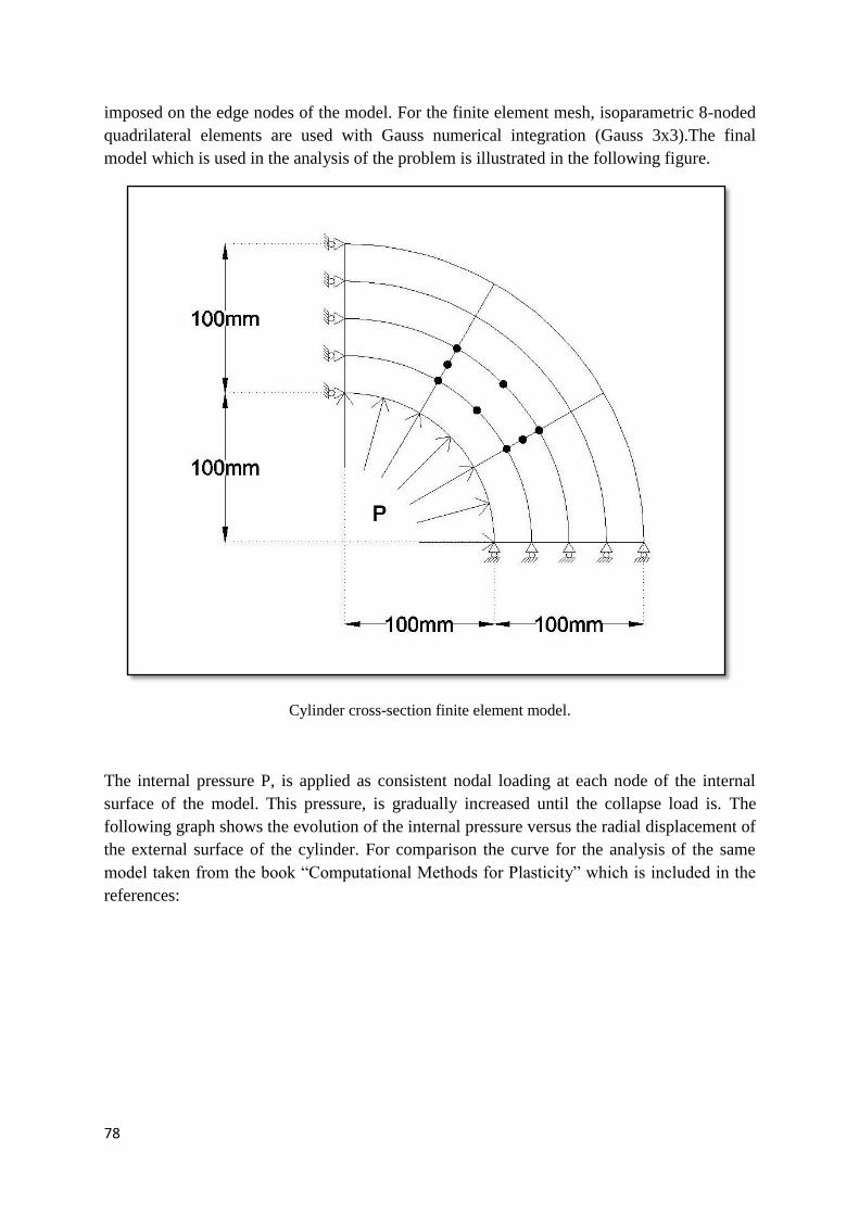
78

imposed on the edge nodes of the model. For the finite element mesh, isoparametric 8-noded

quadrilateral elements are used with Gauss numerical integration (Gauss 3x3).The final

model which is used in the analysis of the problem is illustrated in the following figure.

Cylinder cross-section finite element model.

The internal pressure P, is applied as consistent nodal loading at each node of the internal

surface of the model. This pressure, is gradually increased until the collapse load is. The

following graph shows the evolution of the internal pressure versus the radial displacement of

the external surface of the cylinder. For comparison the curve for the analysis of the same

model taken from the book “Computational Methods for Plasticity” which is included in the

references:

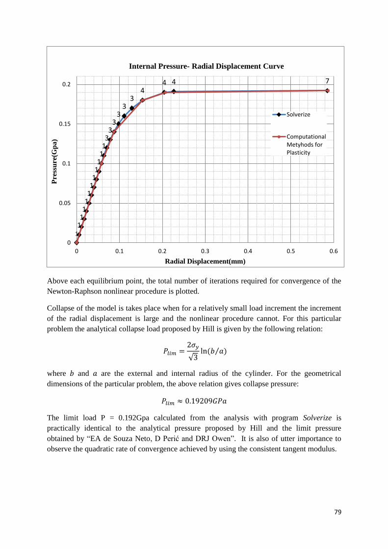
79

Above each equilibrium point, the total number of iterations required for convergence of the

Newton-Raphson nonlinear procedure is plotted.

Collapse of the model is takes place when for a relatively small load increment the increment

of the radial displacement is large and the nonlinear procedure cannot. For this particular

problem the analytical collapse load proposed by Hill is given by the following relation:

√ ( ⁄ )

where and are the external and internal radius of the cylinder. For the geometrical

dimensions of the particular problem, the above relation gives collapse pressure:

The limit load P = 0.192Gpa calculated from the analysis with program Solverize is

practically identical to the analytical pressure proposed by Hill and the limit pressure

obtained by “EA de Souza Neto, D Perić and DRJ Owen”. It is also of utter importance to

observe the quadratic rate of convergence achieved by using the consistent tangent modulus.

1

1 1 1 1 1 1 1 1 1 1 1 3 3

3 3

3 3

4 4 4 7

0

0.05

0.1

0.15

0.2

0 0.1 0.2 0.3 0.4 0.5 0.6

Pre

ssu

re(G

pa

)

Radial Displacement(mm)

Internal Pressure- Radial Displacement Curve

Solverize

ComputationalMetyhods forPlasticity

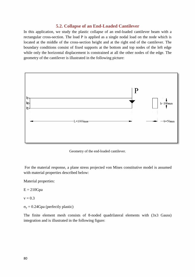
80

5.2. Collapse of an End-Loaded Cantilever

In this application, we study the plastic collapse of an end-loaded cantilever beam with a

rectangular cross-section. The load P is applied as a single nodal load on the node which is

located at the middle of the cross-section height and at the right end of the cantilever. The

boundary conditions consist of fixed supports at the bottom and top nodes of the left edge

while only the horizontal displacement is constrained at all the other nodes of the edge. The

geometry of the cantilever is illustrated in the following picture:

Geometry of the end-loaded cantilever.

For the material response, a plane stress projected von Mises constitutive model is assumed

with material properties described below:

Material properties:

E = 210Gpa

v = 0.3

σy = 0.24Gpa (perfectly plastic)

The finite element mesh consists of 8-noded quadrilateral elements with (3x3 Gauss)

integration and is illustrated in the following figure:

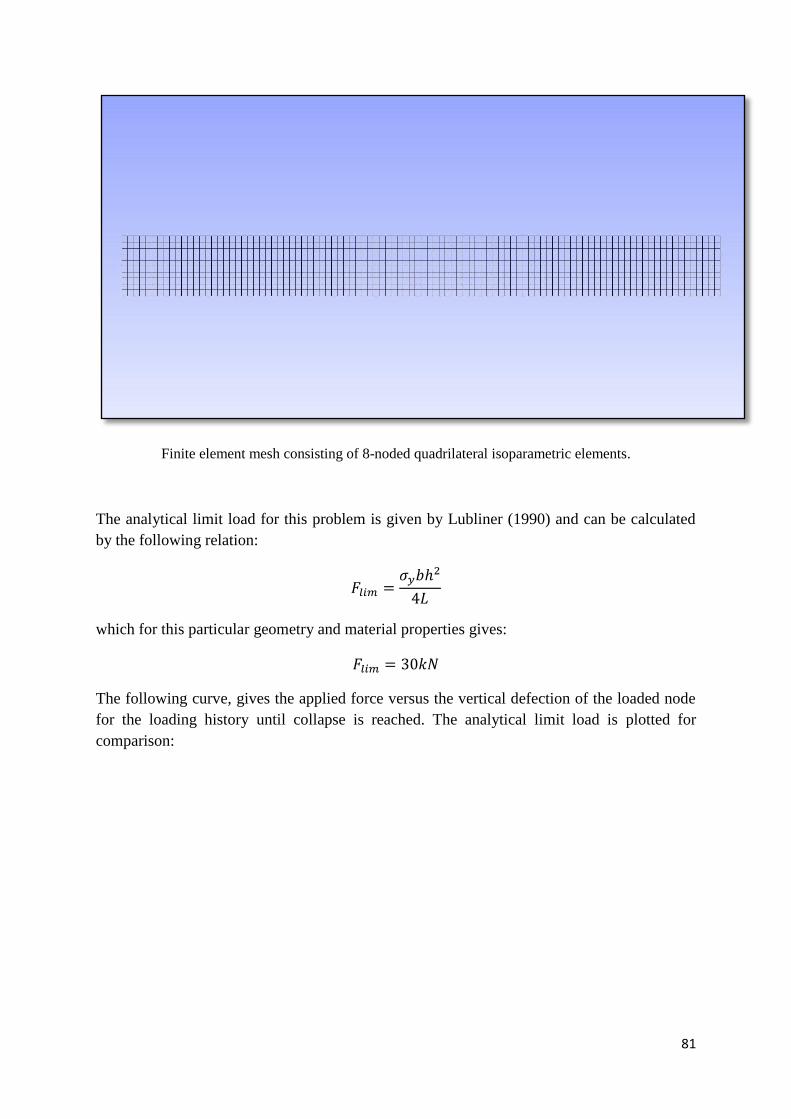
81

Finite element mesh consisting of 8-noded quadrilateral isoparametric elements.

The analytical limit load for this problem is given by Lubliner (1990) and can be calculated

by the following relation:

which for this particular geometry and material properties gives:

The following curve, gives the applied force versus the vertical defection of the loaded node

for the loading history until collapse is reached. The analytical limit load is plotted for

comparison:

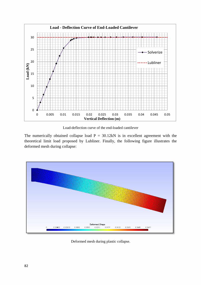
82

Load-deflection curve of the end-loaded cantilever

The numerically obtained collapse load P = 30.12kN is in excellent agreement with the

theoretical limit load proposed by Lubliner. Finally, the following figure illustrates the

deformed mesh during collapse:

Deformed mesh during plastic collapse.

0

5

10

15

20

25

30

0 0.005 0.01 0.015 0.02 0.025 0.03 0.035 0.04 0.045 0.05

Lo

ad

(k

N)

Vertical Deflection (m)

Load - Deflection Curve of End-Loaded Cantilever

Solverize

Lubliner

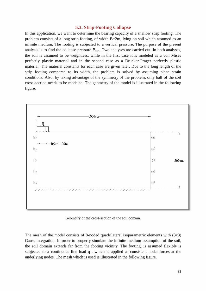
83

5.3. Strip-Footing Collapse

In this application, we want to determine the bearing capacity of a shallow strip footing. The

problem consists of a long strip footing, of width B=2m, lying on soil which assumed as an

infinite medium. The footing is subjected to a vertical pressure. The purpose of the present

analysis is to find the collapse pressure Two analyses are carried out. In both analyses,

the soil is assumed to be weightless, while in the first case it is modeled as a von Mises

perfectly plastic material and in the second case as a Drucker-Prager perfectly plastic

material. The material constants for each case are given later. Due to the long length of the

strip footing compared to its width, the problem is solved by assuming plane strain

conditions. Also, by taking advantage of the symmetry of the problem, only half of the soil

cross-section needs to be modeled. The geometry of the model is illustrated in the following

figure.

Geometry of the cross-section of the soil domain.

The mesh of the model consists of 8-noded quadrilateral isoparametric elements with (3x3)

Gauss integration. In order to properly simulate the infinite medium assumption of the soil,

the soil domain extends far from the footing vicinity. The footing, is assumed flexible is

subjected to a continuous line load q , which is applied as consistent nodal forces at the

underlying nodes. The mesh which is used is illustrated in the following figure.

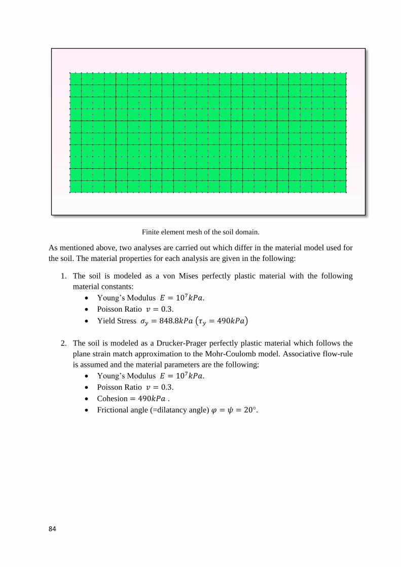
84

Finite element mesh of the soil domain.

As mentioned above, two analyses are carried out which differ in the material model used for

the soil. The material properties for each analysis are given in the following:

1. The soil is modeled as a von Mises perfectly plastic material with the following

material constants:

Young’s Modulus .

Poisson Ratio .

Yield Stress ( )

2. The soil is modeled as a Drucker-Prager perfectly plastic material which follows the

plane strain match approximation to the Mohr-Coulomb model. Associative flow-rule

is assumed and the material parameters are the following:

Young’s Modulus .

Poisson Ratio .

Cohesion .

Frictional angle (=dilatancy angle) .

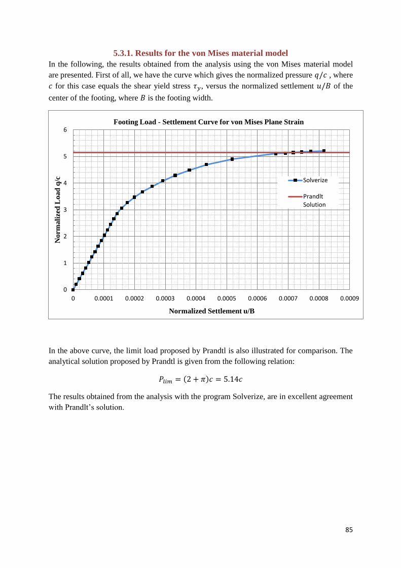
85

5.3.1. Results for the von Mises material model

In the following, the results obtained from the analysis using the von Mises material model

are presented. First of all, we have the curve which gives the normalized pressure , where

for this case equals the shear yield stress , versus the normalized settlement of the

center of the footing, where is the footing width.

In the above curve, the limit load proposed by Prandtl is also illustrated for comparison. The

analytical solution proposed by Prandtl is given from the following relation:

( )

The results obtained from the analysis with the program Solverize, are in excellent agreement

with Prandlt’s solution.

0

1

2

3

4

5

6

0 0.0001 0.0002 0.0003 0.0004 0.0005 0.0006 0.0007 0.0008 0.0009

Norm

ali

zed

Lo

ad

q/c

Normalized Settlement u/B

Footing Load - Settlement Curve for von Mises Plane Strain

Solverize

PrandltSolution

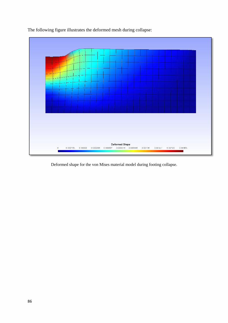
86

The following figure illustrates the deformed mesh during collapse:

Deformed shape for the von Mises material model during footing collapse.

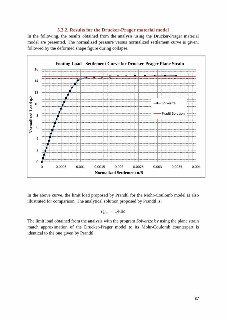
87

5.3.2. Results for the Drucker-Prager material model

In the following, the results obtained from the analysis using the Drucker-Prager material

model are presented. The normalized pressure versus normalized settlement curve is given,

followed by the deformed shape figure during collapse.

In the above curve, the limit load proposed by Prandtl for the Mohr-Coulomb model is also

illustrated for comparison. The analytical solution proposed by Prandtl is:

The limit load obtained from the analysis with the program Solverize by using the plane strain

match approximation of the Drucker-Prager model to its Mohr-Coulomb counterpart is

identical to the one given by Prandtl.

0

2

4

6

8

10

12

14

16

0 0.0005 0.001 0.0015 0.002 0.0025 0.003 0.0035 0.004

Norm

ali

zed

Lo

ad

q/c

Normalized Settlement u/B

Footing Load - Settlement Curve for Drucker-Prager Plane Strain

Solverize

Pradtl Solution

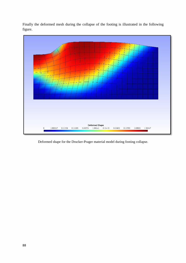
88

Finally the deformed mesh during the collapse of the footing is illustrated in the following

figure.

Deformed shape for the Drucker-Prager material model during footing collapse.

89

References 1. Μ. Παπαδρακάκης. 2001. Ανάλυση Φορέων με τη Μέθοδο των Πεπερασμένων Στοιχείων.

Εκδόσεις Παπασωτηρίου.

2. EA de Souza Neto, D. Perić, DRJ Owen. 2008. Computational Methods for Plasticity:

Theory and Applications. John Wiley & Sons Ltd.

3. Klaus-Jürgen Bathe. 2006. Finite Element Procedures. Klaus-Jürgen Bathe.

4. M. A. Crisfield. 1991. Non-linear Finite Element Analysis of Solids and Structures,

Volume 1: Essentials. John Wiley & Sons Ltd.

5. W. Michael Lai, David Rubin, Erhard Krempl. 2010. Introduction to Continuum

Mechanics, Fourth Edition. Elsevier Ltd.

6. Gerhard A. Hopzapfel. 2000. Nonlinear Solid Mechanics: A Continuum Approach for

Engineering. John Wiley & Sons Ltd.

7. I. M. Smith, D. V. Griffiths. 2004. Programming the Finite Element Method. John Wiley

& Sons Ltd.

8. Gene H. Golub, Charles F. Van Loan. 1996. Matrix Computations. The Johns Hopkins

University Press.

9. Fridtjov Irgens. 2008. Continuum Mechanics. Springer-Verlag Berlin Heidelberg.

10. David M. Potts, Lidija Zdravkovic. 1999. Finite Element Analysis in Geotechnical

Engineering: Theory. Thomas Telford Publishing.

11. A. J. M. Spencer. 1980. Continuum Mechanics. Dover Publications, Inc.

12. A.I. Borisenko, I.E. Tarapov, translated by Richard A. Silverman.1968. Vector and Tensor

Analysis with Applications. Dover Publications, Inc.

13. R. W. Ogden. 1984. Non-Linear Elastic Deformations. Dover Publications, Inc.

14. Helbert Schildt. 2011. Java: The Complete Reference, Eighth Edition. McGraw-Hill.

15. Joshua Bloch. 2008. Effective Java, Second Edition. Addison-Wesley.