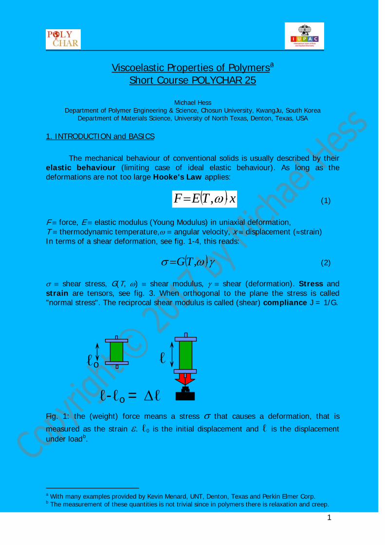
1

Viscoelastic Properties of Polymersa

( ) xTEF ⋅= ω,

Short Course POLYCHAR 25

Michael Hess

Department of Polymer Engineering & Science, Chosun University, KwangJu, South Korea Department of Materials Science, University of North Texas, Denton, Texas, USA

1. INTRODUCTION and BASICS The mechanical behaviour of conventional solids is usually described by their elastic behaviour (limiting case of ideal elastic behaviour). As long as the deformations are not too large Hooke's Law applies:

(1)

F ≡ force, E ≡ elastic modulus (Young Modulus) in uniaxial deformation, T ≡ thermodynamic temperature,ω ≡ angular velocity, x ≡ displacement (≈strain) In terms of a shear deformation, see fig. 1-4, this reads:

( )γωσ ⋅= ,TG (2)

σ ≡ shear stress, G(T, ω) ≡ shear modulus, γ ≡ shear (deformation). Stress and strain are tensors, see fig. 3. When orthogonal to the plane the stress is called "normal stress". The reciprocal shear modulus is called (shear) compliance J = 1/G. Fig. 1: the (weight) force means a stress σ that causes a deformation, that is

measured as the strain ε. ℓ0 is the initial displacement and ℓ is the displacement under loadb

a With many examples provided by Kevin Menard, UNT, Denton, Texas and Perkin Elmer Corp. b The measurement of these quantities is not trivial since in polymers there is relaxation and creep.

.

ℓo

ℓ-ℓo = ∆ℓ

ℓ

2

( ) εσ

λε

⋅=≡→−=

−=−

≡−=∆=

EFEF

x

00

0

00 1,

(3a-d)

There are different types of polymeric materials such as hard viscoelastic

solids orsoft viscoelastic solids and highly viscous liquids (such as pitch) that appear to be a solid on the first glance but that show a very slow flow (creep). Also, the specimen come in a particular shape that should probably not be changed. Consequently, there are different types of stresses and deformations, more or less complex, all of them delivering a corresponding modulus. Examples are extension, compression, shear, torsion, bending (3-point, 4-point), flexing, etc. These mechanical values, however, are correlated. For details see the books of Ferry, or Read and Dean or Menard in "further reading".

Soft materials – the shear modulus is about 107…108 Pa – allow more degrees of freedom in the choice of sample geometry. The Poisson ratio is close to 0.5 so that all extensional viscoelastic functions are correlated with the shear function by the factor 3 (see below).

Hard viscoelastic materials – the shear modulus is about 108…1011 Pa – can principally be investigated with the same kind of equipment, however, some different features may have to be considered when stiffness increases by some orders of magnitude. The stiffness is not only depending on the material and temperature but also on the shape (plate vs. t-bar, for example). The accuracy of a modulus from an experiment can be significantly influenced by the accuracy of the measurement of the shape of the sample. In particular at high values of the modulus care has to be taken that the sample modulus is still much lower than the modulus of structural parts of the measuring equipment, in particular in dynamic experiments.

3

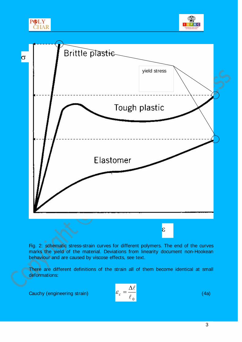
Fig. 2: schematic stress-strain curves for different polymers. The end of the curves marks the yield of the material. Deviations from linearity document non-Hookean behaviour and are caused by viscose effects, see text. There are different definitions of the strain all of them become identical at small deformations:

Cauchy (engineering strain) 0

∆=cε (4a)

σ

ε

yield stress

4

Hencky (true strain) 0

ln

∆=hε (4b)

Kinetic theory of rubber elasticity

−=

2

0031

kε (4c)

Kirchoff strain

−

= 1

21

2

0

Kε (4d)

Murnaghan strain

−=

2

0

121

Mε (4e)

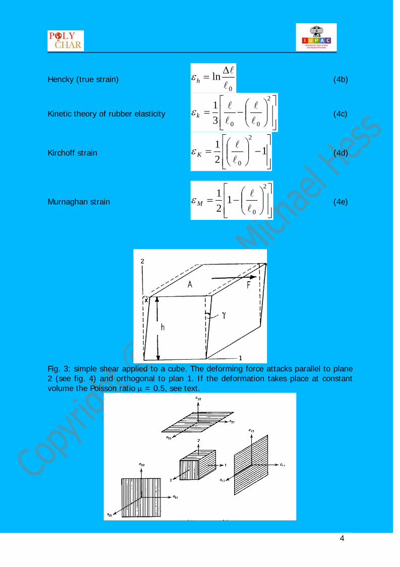
Fig. 3: simple shear applied to a cube. The deforming force attacks parallel to plane 2 (see fig. 4) and orthogonal to plan 1. If the deformation takes place at constant volume the Poisson ratio µ = 0.5, see text.

5

Fig. 4: components of the stress tensor which represent the forces acting from different direction on different faces of a cubical element.

Simple shear is a homogeneous deformation, such that a mass point of the solid with co-ordinates X1, X2, X3 in the undeformed state moves to a point with co-ordinate x1, x2, x3 in the deformed state, with

x1 = X1 + gX2

x2 = X2

x3 = X3

where g is a constant. For the definitions of the non-ultimate mechanical properties of polymers see A. Kaye, R. F. T. Stepto, W. J. Work, J. V. Alemán, A. Ya. Malkin1

γγγ ≈= tan21

. The (simple) shear γ21 that results after application of the stress σ21is given by the quotient x/h, see fig. 3 and fig. 4, and for small deformation angles γ there is:

(5)

The individual stress (respectively deformation) components combine to the total stress σij (strain γij) and can be expressed by the matrix:

=

333231

232221

131211

σσσσσσσσσ

σ ij (6)

In fig. 2 plane 1/3 slides in direction 1 (as indicated in fig. 2) and stress and strain are:

=

−−

−=

0000000

,00

00

21

12

21

12

γγ

γσσ

σ ijij

pp

p

(7a, b)

since only a displacement in strain components the planes 1 and 2 occurs. -p

is an isotropic compressive pressure that occurs on application of the shear stress, and γ12 = γ21.

Dimensional changes caused by longitudinal deformation usually come with changes of the cross section. This is described by the Poisson ratio µ. The Poisson ratio correlates the Young modulus with the shear modulus, respectively the bulk modulus B:

( ) ( )µµ 21312 −=+= BGE (8)

6

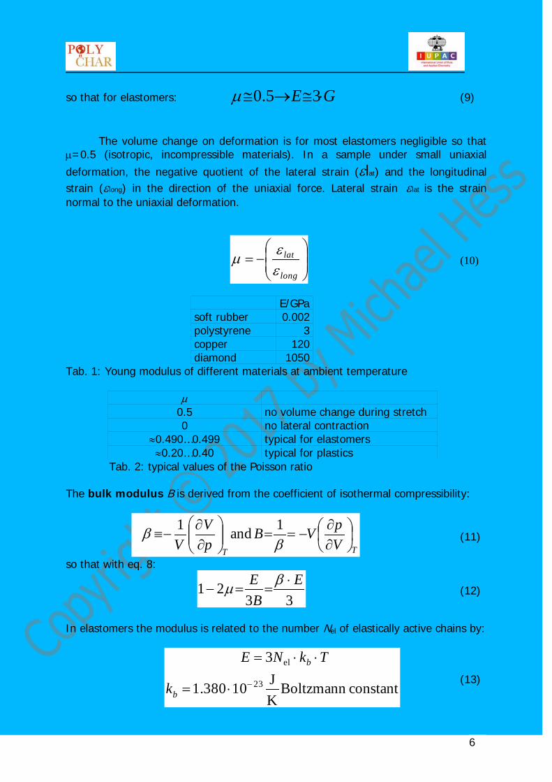
so that for elastomers: GE ⋅≅→≅ 35.0µ (9) The volume change on deformation is for most elastomers negligible so that µ=0.5 (isotropic, incompressible materials). In a sample under small uniaxial deformation, the negative quotient of the lateral strain (εlat) and the longitudinal strain (εlong) in the direction of the uniaxial force. Lateral strain εlat is the strain normal to the uniaxial deformation.

−=

long

lat

εεµ (10)

E/GPa soft rubber 0.002 polystyrene 3 copper 120 diamond 1050

Tab. 1: Young modulus of different materials at ambient temperature

µ 0.5 no volume change during stretch 0 no lateral contraction

≈0.490…0.499 typical for elastomers ≈0.20…0.40 typical for plastics

Tab. 2: typical values of the Poisson ratio The bulk modulus B is derived from the coefficient of isothermal compressibility:

TT VpVB

pV

V

∂∂

−==

∂∂

−≡β

β 1and1 (11)

so that with eq. 8:

3321 E

BE ⋅

==−βµ (12)

In elastomers the modulus is related to the number Nel of elastically active chains by:

constantBoltzmann KJ10380.1

3

23

el

−⋅=

⋅⋅=

b

b

k

TkNE (13)

7

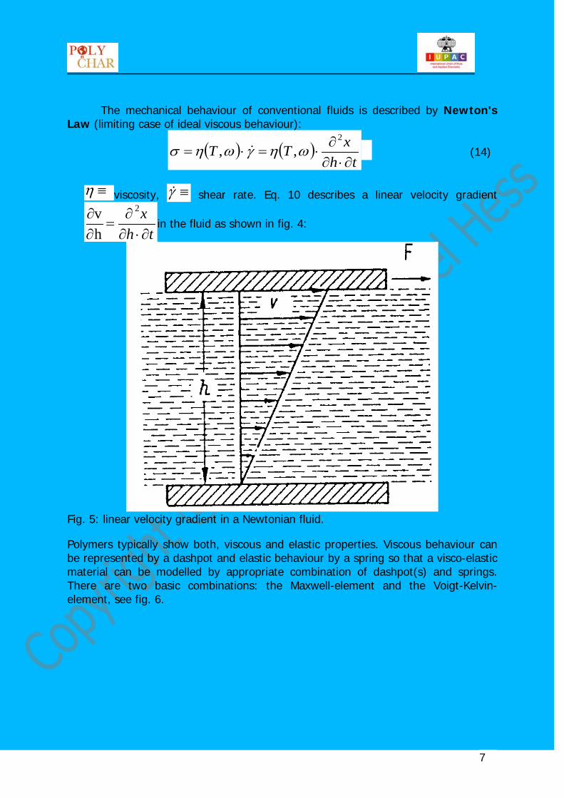
The mechanical behaviour of conventional fluids is described by Newton's

Law (limiting case of ideal viscous behaviour):

( ) ( )th

xTT∂⋅∂

∂⋅=⋅=

2

,, ωηγωησ (14)

≡η viscosity, ≡γ shear rate. Eq. 10 describes a linear velocity gradient

thx∂⋅∂

∂=

∂∂ 2

hv

in the fluid as shown in fig. 4:

Fig. 5: linear velocity gradient in a Newtonian fluid. Polymers typically show both, viscous and elastic properties. Viscous behaviour can be represented by a dashpot and elastic behaviour by a spring so that a visco-elastic material can be modelled by appropriate combination of dashpot(s) and springs. There are two basic combinations: the Maxwell-element and the Voigt-Kelvin-element, see fig. 6.

8

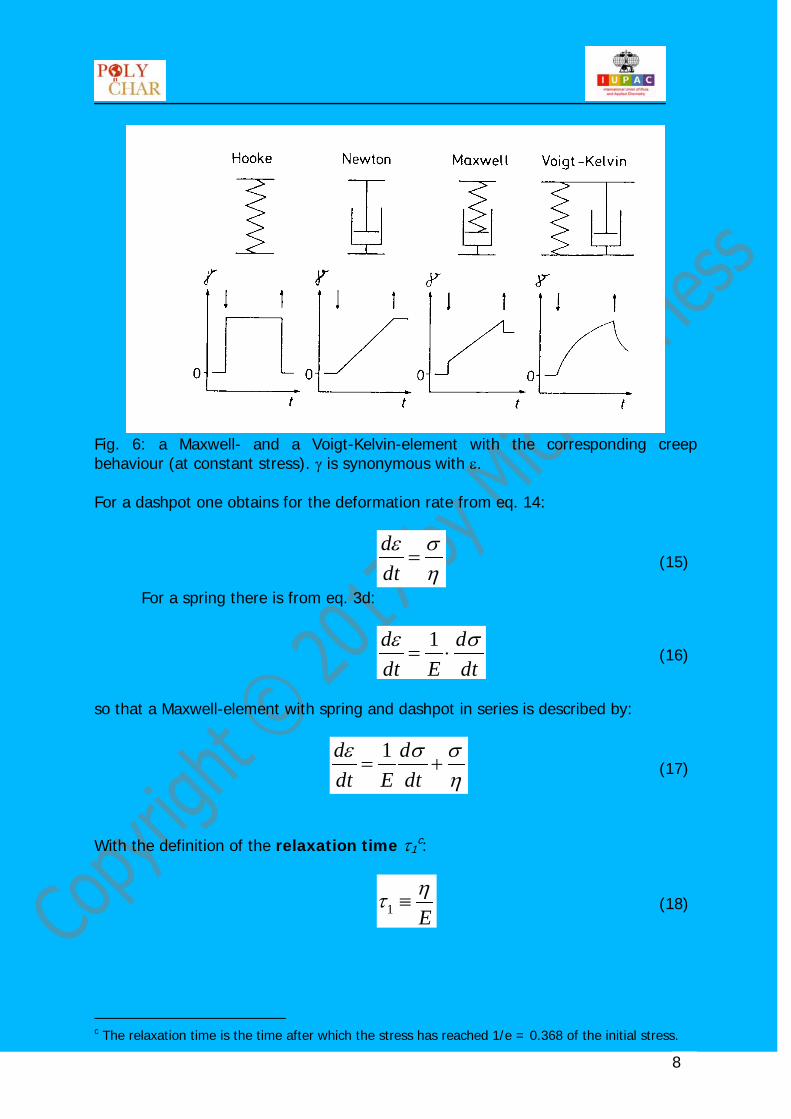
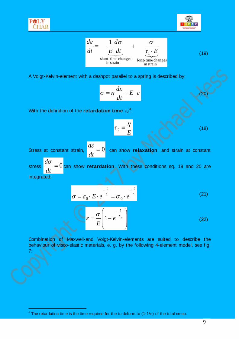
Fig. 6: a Maxwell- and a Voigt-Kelvin-element with the corresponding creep behaviour (at constant stress). γ is synonymous with ε. For a dashpot one obtains for the deformation rate from eq. 14:

ησε

=dtd

(15)

For a spring there is from eq. 3d:

dtd

Edtd σε

⋅=1

(16)

so that a Maxwell-element with spring and dashpot in series is described by:

ησσε

+=dtd

Edtd 1

(17)

With the definition of the relaxation time τ1

c

Eητ ≡1

:

(18)

c The relaxation time is the time after which the stress has reached 1/e = 0.368 of the initial stress.

9

strainin changes time-long

1

strainin changes time-short

1Edt

dEdt

d⋅

+=τ

σσε

(19)

A Voigt-Kelvin-element with a dashpot parallel to a spring is described by:

εεησ ⋅+= Edtd

(20)

With the definition of the retardation time τ2

d

Eητ ≡2

:

(18)

Stress at constant strain, 0=dtdε

, can show relaxation, and strain at constant

stress 0=dtdσ

can show retardation. With these conditions eq. 19 and 20 are

integrated:

11

00ττ σεσtt

eeE−−

⋅=⋅⋅= (21)

−=

−21 τσεt

eE

(22)

Combination of Maxwell-and Voigt-Kelvin-elements are suited to describe the behaviour of visco-elastic materials, e. g. by the following 4-element model, see fig. 7:

d The retardation time is the time required for the to deform to (1-1/e) of the total creep.

10

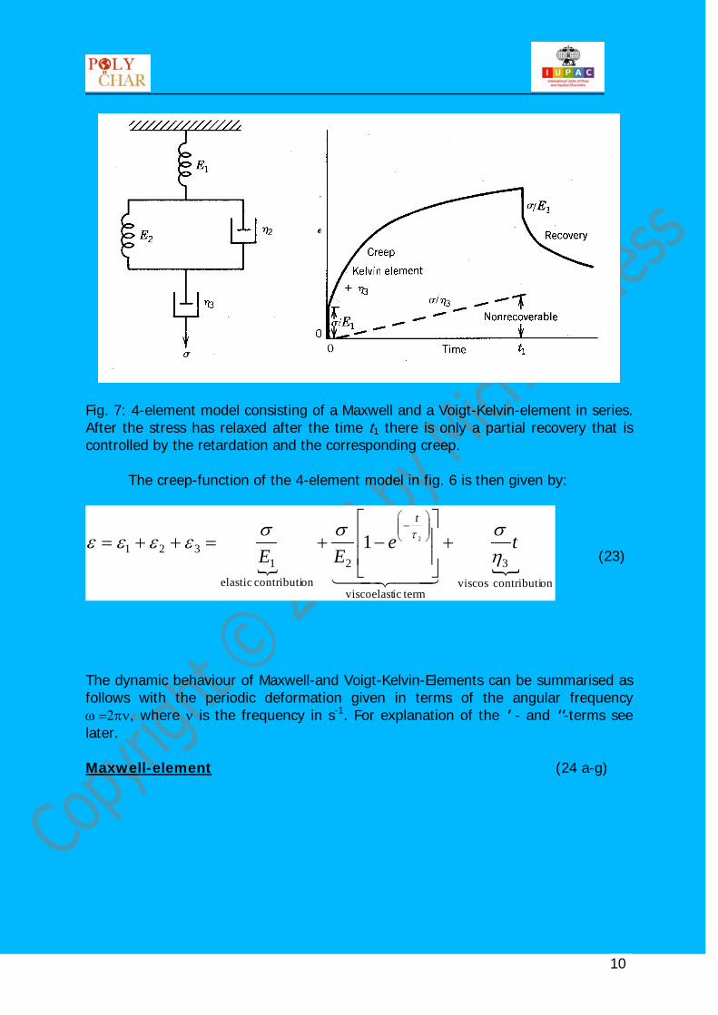
Fig. 7: 4-element model consisting of a Maxwell and a Voigt-Kelvin-element in series. After the stress has relaxed after the time t1 there is only a partial recovery that is controlled by the retardation and the corresponding creep. The creep-function of the 4-element model in fig. 6 is then given by:

oncontributi viscos

3

termicviscoelast

2oncontributi elastic

1321

21 teEE

t

ησσσ

εεεε τ +

−+=++=

−

(23)

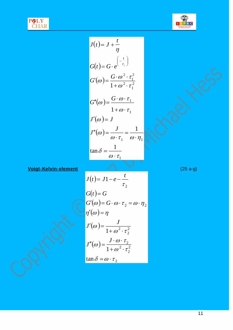
The dynamic behaviour of Maxwell-and Voigt-Kelvin-Elements can be summarised as follows with the periodic deformation given in terms of the angular frequency ω =2πν, where ν is the frequency in s-1. For explanation of the ' - and ''-terms see later. Maxwell-element (24 a-g)

11

( )

( )

( )

( )

( )

( )

1

11

1

1

21

2

21

2

1tan

1

1

1

1

τωδ

ηωτωω

ωτω

τωω

τωτωω

η

τ

⋅=

⋅=

⋅=′′

=′⋅+

⋅⋅=′′

⋅+⋅⋅

=′

⋅=

+=

−

JJ

JJ

GG

GG

eGtG

tJtJ

t

Voigt-Kelvin-element (25 a-g)

( )

( )( )( )

( )

( )

2

22

22

22

2

22

2

tan1

1

1

τωδτωτω

ω

τωω

ηωηηωτωω

τ

⋅=

⋅+⋅⋅

=′′

⋅+=′

=′⋅=⋅⋅=′

=

−−=

JJ

JJ

GGGtG

teJtJ

12

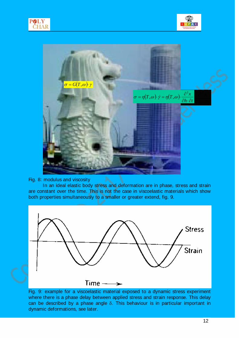
Fig. 8: modulus and viscosity

In an ideal elastic body stress and deformation are in phase, stress and strain are constant over the time. This is not the case in viscoelastic materials which show both properties simultaneously to a smaller or greater extend, fig. 9.

Fig. 9: example for a viscoelastic material exposed to a dynamic stress experiment where there is a phase delay between applied stress and strain response. This delay can be described by a phase angle δ. This behaviour is in particular important in dynamic deformations, see later.

( ) ( )th

xTT∂⋅∂

∂⋅=⋅=

2

,, ωηγωησ

( ) γωσ ⋅= ,TG

( ) ( )th

xTT∂⋅∂

∂⋅=⋅=

2

,, ωηγωησ

( ) γωσ ⋅= ,TG

13

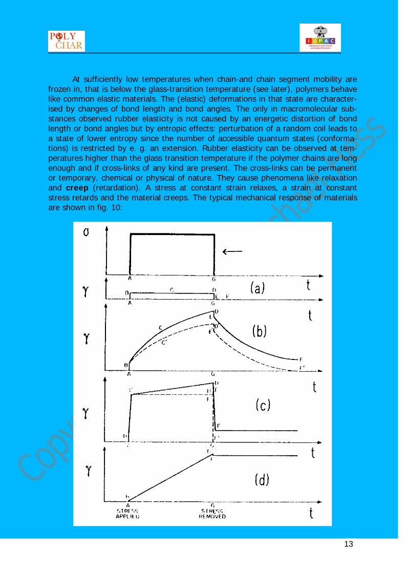
At sufficiently low temperatures when chain-and chain segment mobility are frozen in, that is below the glass-transition temperature (see later), polymers behave like common elastic materials. The (elastic) deformations in that state are character-ised by changes of bond length and bond angles. The only in macromolecular sub-stances observed rubber elasticity is not caused by an energetic distortion of bond length or bond angles but by entropic effects: perturbation of a random coil leads to a state of lower entropy since the number of accessible quantum states (conforma-tions) is restricted by e. g. an extension. Rubber elasticity can be observed at tem-peratures higher than the glass transition temperature if the polymer chains are long enough and if cross-links of any kind are present. The cross-links can be permanent or temporary, chemical or physical of nature. They cause phenomena like relaxation and creep (retardation). A stress at constant strain relaxes, a strain at constant stress retards and the material creeps. The typical mechanical response of materials are shown in fig. 10:

14

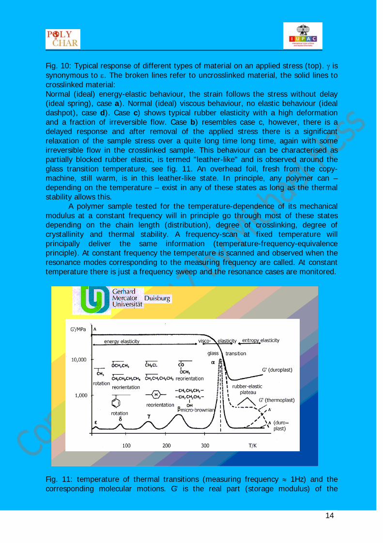
Fig. 10: Typical response of different types of material on an applied stress (top). γ is synonymous to ε. The broken lines refer to uncrosslinked material, the solid lines to crosslinked material: Normal (ideal) energy-elastic behaviour, the strain follows the stress without delay (ideal spring), case a). Normal (ideal) viscous behaviour, no elastic behaviour (ideal dashpot), case d). Case c) shows typical rubber elasticity with a high deformation and a fraction of irreversible flow. Case b) resembles case c, however, there is a delayed response and after removal of the applied stress there is a significant relaxation of the sample stress over a quite long time long time, again with some irreversible flow in the crosslinked sample. This behaviour can be characterised as partially blocked rubber elastic, is termed "leather-like" and is observed around the glass transition temperature, see fig. 11. An overhead foil, fresh from the copy-machine, still warm, is in this leather-like state. In principle, any polymer can – depending on the temperature – exist in any of these states as long as the thermal stability allows this. A polymer sample tested for the temperature-dependence of its mechanical modulus at a constant frequency will in principle go through most of these states depending on the chain length (distribution), degree of crosslinking, degree of crystallinity and thermal stability. A frequency-scan at fixed temperature will principally deliver the same information (temperature-frequency-equivalence principle). At constant frequency the temperature is scanned and observed when the resonance modes corresponding to the measuring frequency are called. At constant temperature there is just a frequency sweep and the resonance cases are monitored.

Fig. 11: temperature of thermal transitions (measuring frequency ≈ 1Hz) and the corresponding molecular motions. G' is the real part (storage modulus) of the

15

complex shear modulus, Λ is the logarithmic decrement. For explanation see text and fig. 18-20.

There is a direct relation of the viscoelastic properties of a polymer and

molecular motions, in particular cooperative motions. This is caused by the fact that each deformation of a polymer chain changes its equilibrium conformation, hence giving rise to an entropy-driven tendency to restore the initial state. There are always four parts in the temperature-modulus curve of an amorphous polymer: the metastable glassy solid (frozen liquid) at low temperatures followed by the glass-rubber (or brittle-tough-) transition, the more or less pronounced rubber-elastic plateau, and finally the terminal flow range. The first transition in fig. 8 coming down from high temperatures is termed α transition. In semi-crystalline polymers this is the crystallisation/melting process. In amorphous polymers – such as in fig.8 – the glass transition temperature is the strongest transition (α-relaxation). These transitions are also called relaxations since – coming from low temperatures – they describe the onset of the molecular motion as indicated in fig. 8. In particular the glass transition indicates the onset of cooperative chain-segment motions (about 5 chain segments) and is a continuous transition leading from a solid-like state to a liquid-like state (or vice versa). The glass transition is not an equilibrium transition, see below. As a matter of fact there is no "the" glass transition temperature since there is an infinite number of glass states (hence glas transition temperatures) depending on the thermal history. Annealing changes the physical properties of a glass.

The relaxation behaviour can be monitored at a fixed temperature with a frequency sweep or it can be monitored at a fixed frequency but with a temperature sweep. In the first case resonance is observed when the applied frequency matches a corresponding molecular motion at this temperature, in the second case resonance is observed when the energy provided by the applied temperature fits in with a molecular motion that matches with the chosen frequency. This reflects a time-temperature relation – Boltzmann's time-temperature superposition principle (TTS), see fig. XXX – this, however, is not generally valid, only if all relaxation processes are affected by the temperature in the same way. Only in these cases time and temperature are equivalent. There are numerous examples where there are deviations from TTS, see fig. 13.

The temperature-dependence of the relaxation processes mentioned above can be described by the Williams-Landel-Ferry equation (WLF)2 as long as the restriction mentioned does not apply. The (semi-empirical) WLF equation can be derived using the free volume theory, and a quantitative description is frequently possible in the melt in a temperature range from Tg to Tg+100 K. The derivation goes back to the early work of Doolittle3 on the viscosity of non-associated pure liquids. The importance of a relation like the WLF equation becomes clear recalling the fact that the experimental techniques usually only cover a rather narrow time slot, e. g. 100s…105 s ( corresponding to a frequency range). The time-temperature superposition principle allows an estimate of the relaxation behaviour and related properties of polymers – such as the melt viscosity – over a wide temperature range (e.g. 10-14 hrs…102 hrs) with the WLF-equation and the shift factor.

16

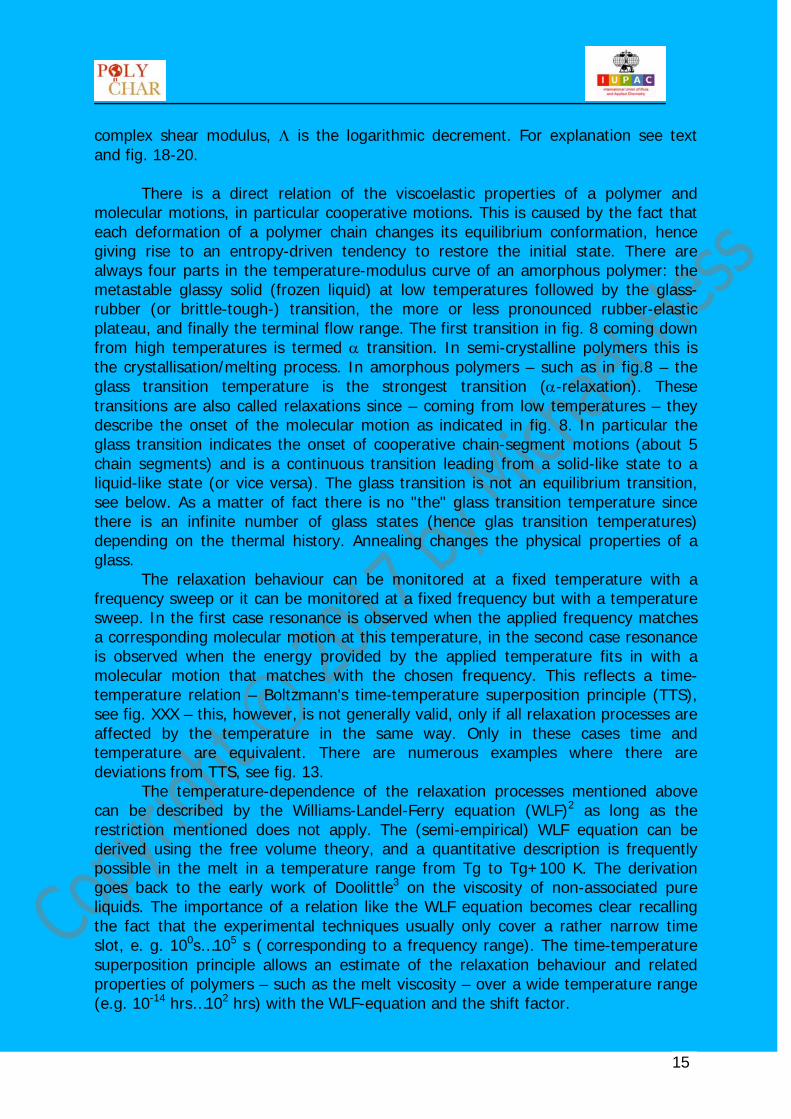
Fig. 12: TTS: superposition of the individual relaxation curves at different temperatures as indicated on the left to one master curve at 25°C on the right. The insert shows the temperature-dependence of the shift parameter that is required to make all curves fit into one master curve.

Considered a certain generalised transition temperature T0 (frequently the glass transition temperature), AT is called the reduced variables shift factor, where t0 is the time required for the transition and η0 the corresponding viscosity. The other values are then valid for a different state.

==

00

lnlnlnttATη

η (26)

AT is not only related with the viscosity but with many other time-dpendent quantities at the transition temperature respectively another temperature, see below.

17

( )

( )TsT

TsTAtt

TgTTgT

Att

tss

C

C

tgg

−+−

−==

=

−+−

−==

=

6.10186.8lglglg

:lyrespective

6.5144.17

lglglg

2

1

ηη

ηη

(27a, b)

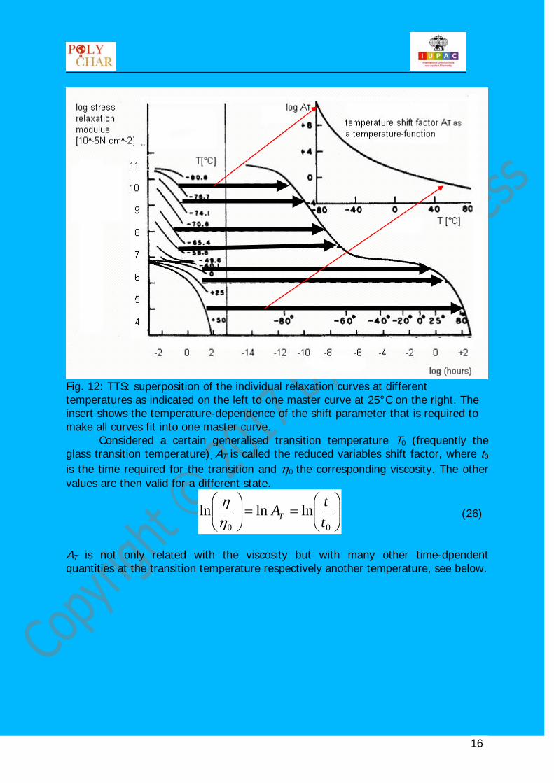
Ts [K]= (Tg + 50) The index s indicates the situation at an arbitrary temperature up to 50 K above Tg. The numerical constants are empirical and valid for a number of linear amorphous polymers more or less independent of their chemical nature. The constants C1 and C2 depend on the polymer. The "universal" constants are C1=17.44 and C2=51.6 and give good results for many polymers. Some examples were listed by Aklonis and McKnight4:

C1 C2 Tg/K polyisbutylene 16.6 104 202 Natural rubber 16.7 53.6 200 Polyurethane (elastomer) 15.6 32.6 238 polystyrene 14.5 50.4 373 Poly(ethyl methacrylate) 17.6 65.5 335

Tab. 3: WLF-constants and Tg from Aklonis and McKnight In this way, the WLF-equation enables a determination of the frequency dependence of a determination of a physical entity of polymers that depends on the free volume, such as the glass transition temperature, the determination of which is frequency dependent. For example an increase of the measuring frequency by a factor 10 (or a decrease of the time frame by a factor of 10) near Tg the glass-transition temperature is found about 3 K higher: From eq. 27a one obtains:

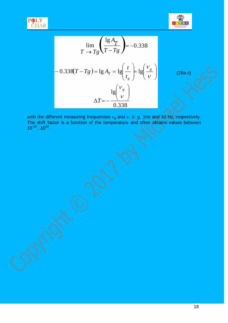
18

( )( )

338.0

lg

lglglg338.0

338.0lg

lim

−=∆

=

==−−

−=−→

νν

νν

g

g

gT

T

ttATgT

TgTTA

TgT

(28a-c)

with the different measuring frequencies νg and ν, e. g. 1Hz and 10 Hz, respectively. The shift factor is a function of the temperature and often obtains values between 10-10…1010.

19

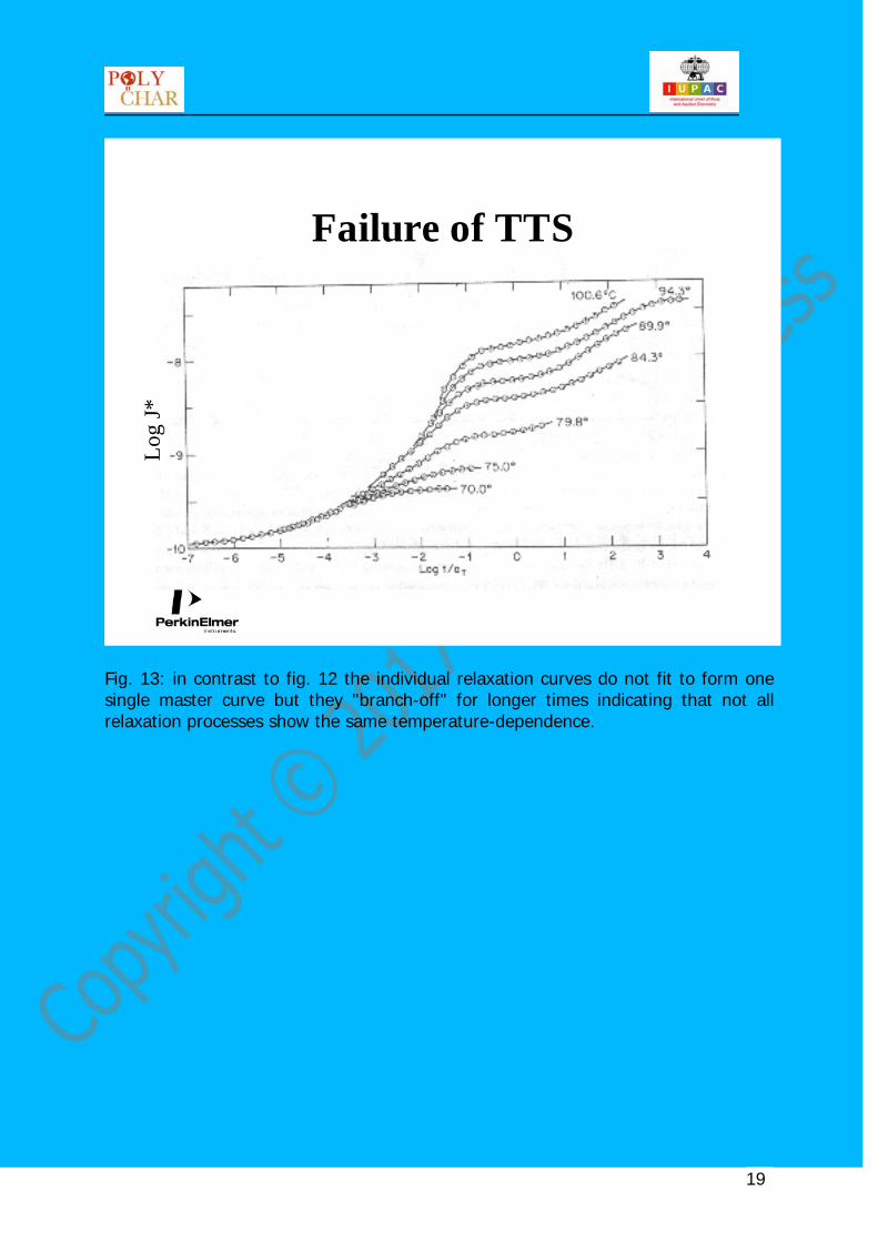
Failure of TTS

Log

J*

Fig. 13: in contrast to fig. 12 the individual relaxation curves do not fit to form one single master curve but they "branch-off" for longer times indicating that not all relaxation processes show the same temperature-dependence.

20

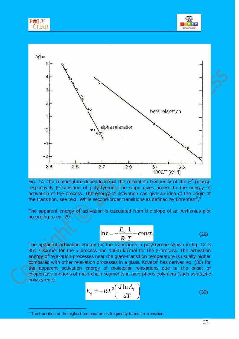
Fig. 14: the temperature-dependence of the relaxation frequency of the αe

.1ln constTR

Et a +−=

-(glass), respectively β-transition of polystyrene. The slope gives access to the energy of activation of the process. The energy of activation can give an idea of the origin of the transition, see text. While second-order transitions as defined by Ehrenfest5,6 The apparent energy of activation is calculated from the slope of an Arrhenius plot according to eq. 29:

(29)

The apparent activation energy for the transitions in polystyrene shown in fig. 13 is 351.7 kJ/mol for the α-process and 146.5 kJ/mol for the β-process. The activation energy of relaxation processes near the glass-transition temperature is usually higher compared with other relaxation processes in a glass. Kovacs7 has derived eq. (30) for the apparent activation energy of molecular relaxations due to the onset of cooperative motions of main-chain segments in amorphous polymers (such as atactic polystyrene):

−=

dTAd

RTE Ta

ln2 (30)

e The transition at the highest temperature is frequently termed α-transition

21

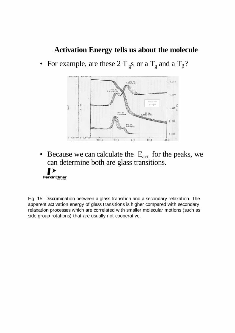
Activation Energy tells us about the molecule

• For example, are these 2 T gs or a Tg and a Tβ?

• Because we can calculate the Eact for the peaks, we can determine both are glass transitions.

Elastomer Sa mple

Fig. 15: Discrimination between a glass transition and a secondary relaxation. The apparent activation energy of glass transitions is higher compared with secondary relaxation processes which are correlated with smaller molecular motions (such as side group rotations) that are usually not cooperative.

22

The melting transition – a first order transition – is not frequency depending. In cases where it is difficult to measure a sample beyond its melting transition because the sample shape disintegrates because of the melt flow, torsional braid-analysis or a comparable technique might be used to determine the transition temperature. This technique analyses the mechanical properties of the polymer supported by an inert material. This can be a textile material soaked with the sample, a thin metal foil metal (transitions in lacquer layers or polymer surface layers of a few micrometer thickness can be analysed) or braids of glass threads or fabric can be used. However, care has to be taken because interactions of the substrate with the support can influence the transition (temperature, strength, etc.). The glass-transition temperature is said to be the temperature at which the motion of groups of segments (such as a few repetition units) freeze in a cooperative way, where the viscosity diverges etc.. There are three very different theories approaching the phenomenon of the glass transition. These are summarised in tab. 4 with their advantages and disadvantages. The criteria for a second order transition according to Ehrenfest are usually not fulfilled and there is a strong evidence for its kinetic character.

advantages disadvantages thermodynamic theory8 Variation of Tg with

molecular mass, plasticizer and cross-link density are predicted with some accuracy

A true second order transition is predicted but poorly defined Infinite time scale required for measurements

kinetic theory2, 3 Frequency-dependence of Tg are well predicted Heat capacities can be determined

No Tg predicted for infinite time scale

Free-volume theory9,10,11 Time-temperature super-position principle Expansivity (below and above) can be related with Tg

The actual molecular motions are poorly defined

Fox and Flory10 have shown that the (number-average) molar mass of a

polymer significantly influences the glass transition temperature, so that polymerization and cross-linking processe (gelation) are reflected by Tg, e. g. during the curing process of a thermoset.

ngg M

KTT −= ∞ (31)

23

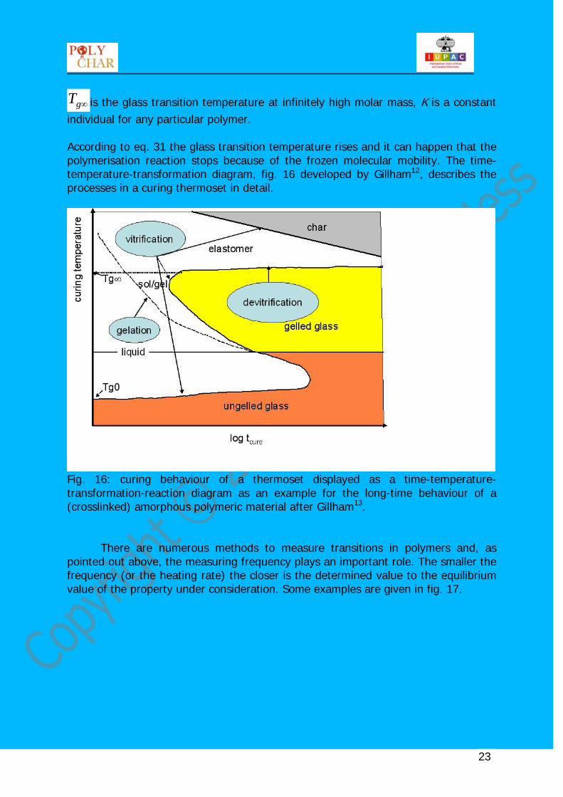
∞gT is the glass transition temperature at infinitely high molar mass, K is a constant individual for any particular polymer. According to eq. 31 the glass transition temperature rises and it can happen that the polymerisation reaction stops because of the frozen molecular mobility. The time-temperature-transformation diagram, fig. 16 developed by Gillham12, describes the processes in a curing thermoset in detail.

Fig. 16: curing behaviour of a thermoset displayed as a time-temperature-transformation-reaction diagram as an example for the long-time behaviour of a (crosslinked) amorphous polymeric material after Gillham13. There are numerous methods to measure transitions in polymers and, as pointed out above, the measuring frequency plays an important role. The smaller the frequency (or the heating rate) the closer is the determined value to the equilibrium value of the property under consideration. Some examples are given in fig. 17.

24

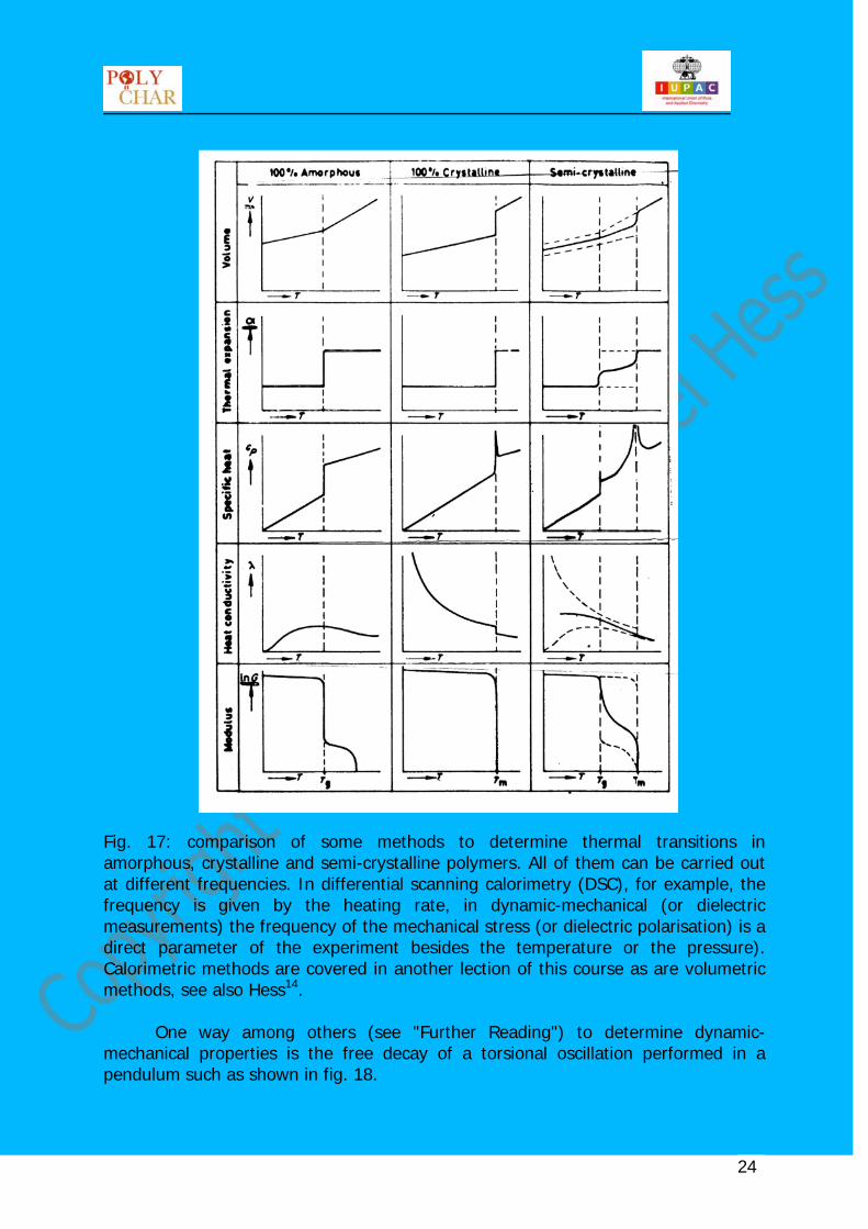
Fig. 17: comparison of some methods to determine thermal transitions in amorphous, crystalline and semi-crystalline polymers. All of them can be carried out at different frequencies. In differential scanning calorimetry (DSC), for example, the frequency is given by the heating rate, in dynamic-mechanical (or dielectric measurements) the frequency of the mechanical stress (or dielectric polarisation) is a direct parameter of the experiment besides the temperature or the pressure). Calorimetric methods are covered in another lection of this course as are volumetric methods, see also Hess14. One way among others (see "Further Reading") to determine dynamic-mechanical properties is the free decay of a torsional oscillation performed in a pendulum such as shown in fig. 18.

25

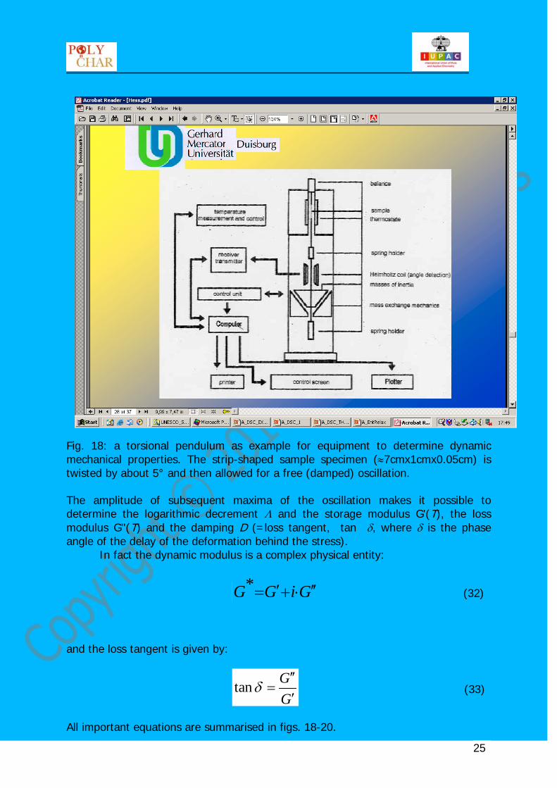
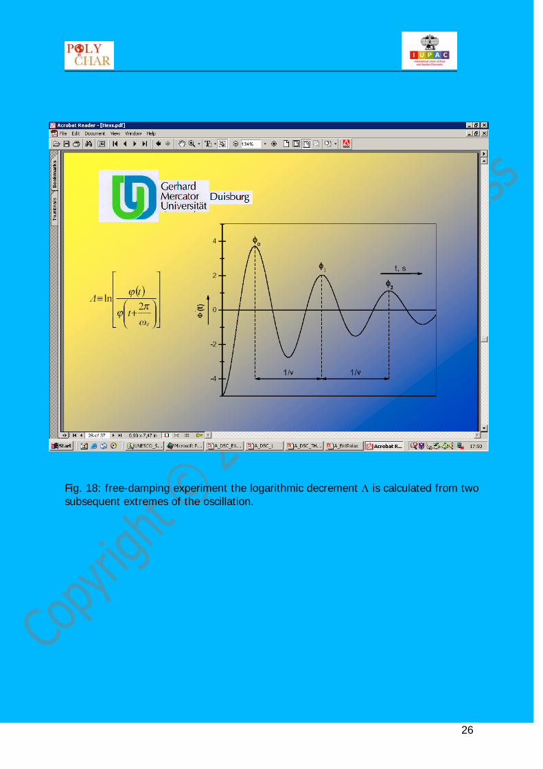
Fig. 18: a torsional pendulum as example for equipment to determine dynamic mechanical properties. The strip-shaped sample specimen (≈7cmx1cmx0.05cm) is twisted by about 5° and then allowed for a free (damped) oscillation. The amplitude of subsequent maxima of the oscillation makes it possible to determine the logarithmic decrement Λ and the storage modulus G'(T), the loss modulus G''(T) and the damping D (=loss tangent, tan δ, where δ is the phase angle of the delay of the deformation behind the stress). In fact the dynamic modulus is a complex physical entity:

GiGG ′′⋅+′=* GiGG ′′⋅+′=* (32)

and the loss tangent is given by:

GG

′′′

=δtan (33)

All important equations are summarised in figs. 18-20.

26

Fig. 18: free-damping experiment the logarithmic decrement Λ is calculated from two subsequent extremes of the oscillation.

27

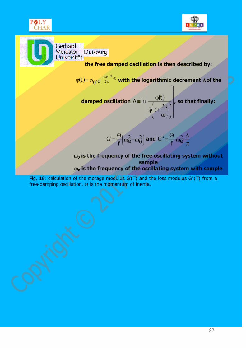
Fig. 19: calculation of the storage modulus G'(T) and the loss modulus G''(T) from a free-damping oscillation. Θ is the momentum of inertia.

28

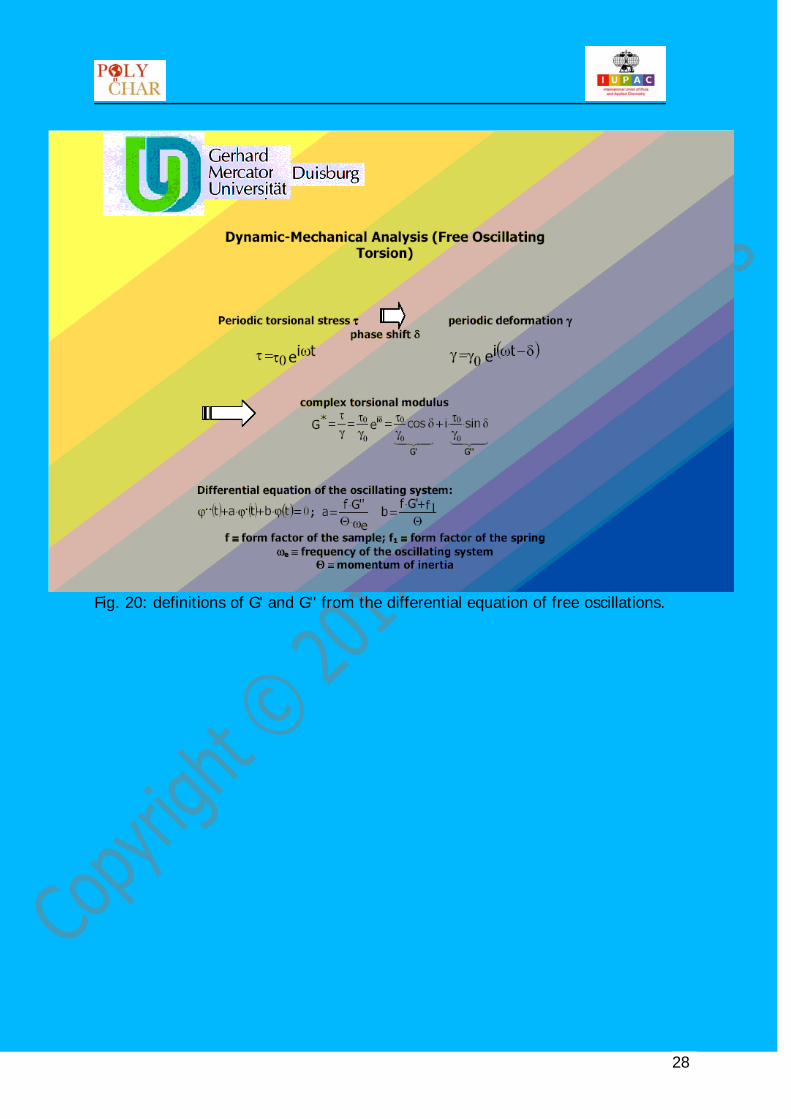
Fig. 20: definitions of G' and G'' from the differential equation of free oscillations.

29

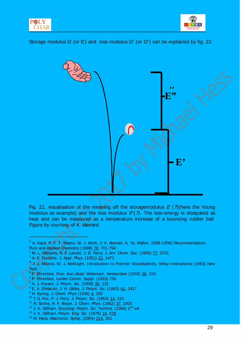
Storage modulus G' (or E') and loss modulus G'' (or G'') can be explained by fig. 21: Fig. 21: visualisation of the meaning off the storagemodulus E' (T)(here the Young modulus as example) and the loss modulus E''(T). The loss-energy is dissipated as heat and can be measured as a temperature increase of a bouncing rubber ball. Figure by courtesy of K. Menard. 1 A. Kaye, R. F. T. Stepto, W. J. Work, J. V. Alemán, A. Ya. Malkin, 1998 IUPAC Recommendation, Pure and Applied Chemistry (1998) 70, 701-754 2 M. L. Williams, R. F. Landel, J. D. Ferry, J. Am. Chem. Soc. (1955) 77, 3701 3 A. K. Doolittle, J. Appl. Phys. (1951) 22, 1471 4 J. J. Aklonis, W. J. McKnight, Introduction to Polymer Viscoelasticity, Wiley-Interscience (1983) New York 5 P. Ehrenfest, Proc. Kon.Akad. Wetensch. Amsterdam (1933) 36, 153 6 P. Ehrenfest, Leiden Comm. Suppl. (1933) 756 7 A. J. Kovacs, J. Polym. Sci. (1958) 30, 131 8 E. A. DiMarzio, J. H. Gibbs, J. Polym. Sci. (1963) A1, 1417 9 H. Eyring, J. Chem. Phys (1936) 4, 283 10 T.G. Fox, P. J. Flory, J. Polym. Sci. (1954) 14, 315 11 R. Simha, R. F. Boyer, J. Chem. Phys. (1962) 37, 1003 12 J. K. Gillham, Encyclop. Polym. Sci. Technol. (1986) 2nd ed. 13 J. K. Gillham, Polym. Eng. Sci. (1979) 19, 676 14 M. Hess, Macromol. Symp. (2004) 214, 361

E”

E’

,,

31

FURTHER READING Kevin P. Menard, Dynamic-Mechanical Analysis, CRC-Press (1999) Boca Raton W. Brostow, Performance of Plastics, Carl Hanser Verlag (2000) Munich I. M. Ward, Mechanical Properties of Solid Polymers, Wiley (1983) New York J. J. Aklonis, W. J. McKnight, Introduction to Polymer Viscoelasticity, Wiley-Interscience (1983) New York N. W. Tschloegl, The Theory of Viscoelastic Behaviour, Acad. Press (1981) New York D. Ferry, Viscoelastic Properties of Polymers, Wiley (1980) New York B. E. Read, G. D. Dean, the Determination of Dynamic Properties of Polymers and Composites, Hilger (1978) Bristol L. E. Nielsen, Polymer Rheology, Dekker (1977) New York L. E. Nielsen, Mechanical Properties of Polymers, Dekker (1974) New York L. E. Nielsen, Mechanical Properties of Polymers and Composites Vol. I & II, Dekker (1974) New York A. V. Tobolsky, Properties and Structure of Polymers, Wiley (1960) New York