Eigenvalues and eigenvectors of a matrix - Dublin …dmackey/lectures/Eigenvals.pdfEigenvalues and...

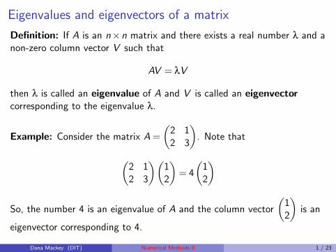
Eigenvalues and eigenvectors of a matrix

Definition: If A is an n×n matrix and there exists a real number λ and anon-zero column vector V such that

AV = λV

then λ is called an eigenvalue of A and V is called an eigenvectorcorresponding to the eigenvalue λ.

Example: Consider the matrix A =

(2 12 3

). Note that

(2 12 3

)(12

)= 4

(12

)

So, the number 4 is an eigenvalue of A and the column vector

(12

)is an

eigenvector corresponding to 4.

Dana Mackey (DIT) Numerical Methods II 1 / 23

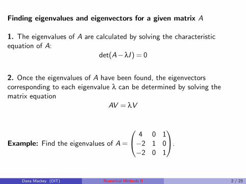
Finding eigenvalues and eigenvectors for a given matrix A

1. The eigenvalues of A are calculated by solving the characteristicequation of A:

det(A−λI ) = 0

2. Once the eigenvalues of A have been found, the eigenvectorscorresponding to each eigenvalue λ can be determined by solving thematrix equation

AV = λV

Example: Find the eigenvalues of A =

4 0 1−2 1 0−2 0 1

.


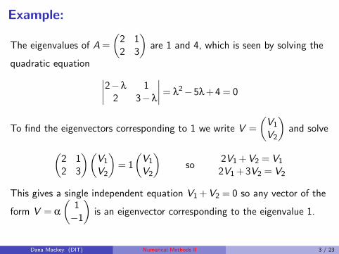
Example:

The eigenvalues of A =

(2 12 3

)are 1 and 4, which is seen by solving the

quadratic equation ∣∣∣∣2−λ 12 3−λ

∣∣∣∣= λ2−5λ + 4 = 0

To find the eigenvectors corresponding to 1 we write V =

(V1

V2

)and solve

(2 12 3

)(V1

V2

)= 1

(V1

V2

)so

2V1 +V2 = V1

2V1 + 3V2 = V2

This gives a single independent equation V1 +V2 = 0 so any vector of the

form V = α

(1−1

)is an eigenvector corresponding to the eigenvalue 1.


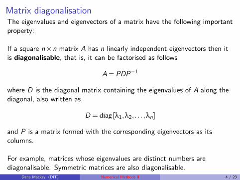
Matrix diagonalisationThe eigenvalues and eigenvectors of a matrix have the following importantproperty:

If a square n×n matrix A has n linearly independent eigenvectors then itis diagonalisable, that is, it can be factorised as follows

A = PDP−1

where D is the diagonal matrix containing the eigenvalues of A along thediagonal, also written as

D = diag [λ1,λ2, . . . ,λn]

and P is a matrix formed with the corresponding eigenvectors as itscolumns.

For example, matrices whose eigenvalues are distinct numbers arediagonalisable. Symmetric matrices are also diagonalisable.


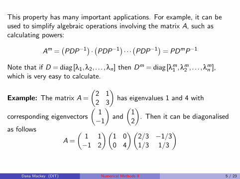
This property has many important applications. For example, it can beused to simplify algebraic operations involving the matrix A, such ascalculating powers:

Am =(PDP−1

)·(PDP−1

)· · ·(PDP−1

)= PDmP−1

Note that if D = diag [λ1,λ2, . . . ,λn] then Dm = diag [λm1 ,λ

m2 , . . . ,λ

mn ],

which is very easy to calculate.

Example: The matrix A =

(2 12 3

)has eigenvalues 1 and 4 with

corresponding eigenvectors

(1−1

)and

(12

). Then it can be diagonalised

as follows

A =

(1 1−1 2

)(1 00 4

)(2/3 −1/31/3 1/3

)


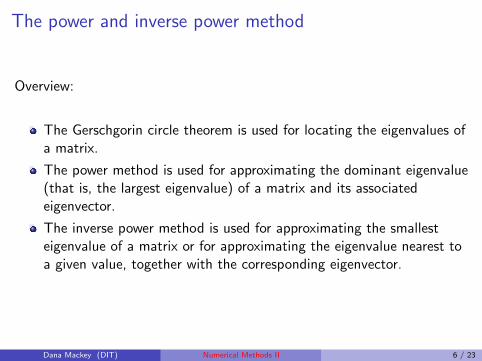
The power and inverse power method

Overview:

The Gerschgorin circle theorem is used for locating the eigenvalues ofa matrix.

The power method is used for approximating the dominant eigenvalue(that is, the largest eigenvalue) of a matrix and its associatedeigenvector.

The inverse power method is used for approximating the smallesteigenvalue of a matrix or for approximating the eigenvalue nearest toa given value, together with the corresponding eigenvector.


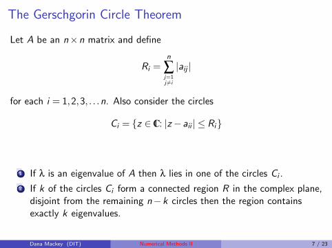
The Gerschgorin Circle Theorem

Let A be an n×n matrix and define

Ri =n

∑j=1j 6=i

|aij |

for each i = 1,2,3, . . .n. Also consider the circles

Ci = {z ∈ Cl : |z−aii | ≤ Ri}

1 If λ is an eigenvalue of A then λ lies in one of the circles Ci .

2 If k of the circles Ci form a connected region R in the complex plane,disjoint from the remaining n−k circles then the region containsexactly k eigenvalues.


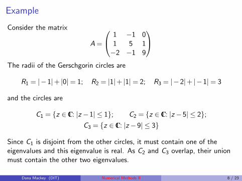
Example

Consider the matrix

A =

1 −1 01 5 1−2 −1 9

The radii of the Gerschgorin circles are

R1 = |−1|+ |0|= 1; R2 = |1|+ |1|= 2; R3 = |−2|+ |−1|= 3

and the circles are

C1 = {z ∈ Cl : |z−1| ≤ 1}; C2 = {z ∈ Cl : |z−5| ≤ 2};C3 = {z ∈ Cl : |z−9| ≤ 3}

Since C1 is disjoint from the other circles, it must contain one of theeigenvalues and this eigenvalue is real. As C2 and C3 overlap, their unionmust contain the other two eigenvalues.


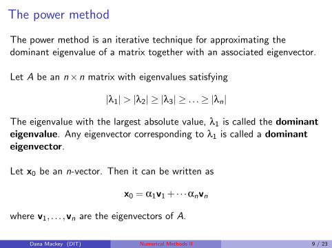
The power method

The power method is an iterative technique for approximating thedominant eigenvalue of a matrix together with an associated eigenvector.

Let A be an n×n matrix with eigenvalues satisfying

|λ1|> |λ2| ≥ |λ3| ≥ . . .≥ |λn|

The eigenvalue with the largest absolute value, λ1 is called the dominanteigenvalue. Any eigenvector corresponding to λ1 is called a dominanteigenvector.

Let x0 be an n-vector. Then it can be written as

x0 = α1v1 + · · ·αnvn

where v1, . . . ,vn are the eigenvectors of A.


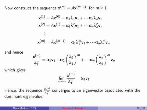
Now construct the sequence x(m) = Ax(m−1), for m ≥ 1.

x(1) = Ax(0) = α1λ1v1 + · · ·αnλnvn

x(2) = Ax(1) = α1λ21v1 + · · ·αnλ

2nvn

...

x(m) = Ax(m−1) = α1λm1 v1 + · · ·αnλ

mn vn

and hencex(m)

λm1

= α1v1 + α2

(λ2

λ1

)m

+ · · ·αn

(λn

λ1

)m

vn

which gives

limm→∞

x(m)

λm1

= α1v1

Hence, the sequence x(m)

λm1

converges to an eigenvector associated with the

dominant eigenvalue.


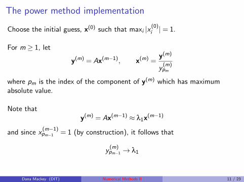
The power method implementation

Choose the initial guess, x(0) such that maxi |x(0)i |= 1.

For m ≥ 1, let

y(m) = Ax(m−1), x(m) =y(m)

y(m)pm

where pm is the index of the component of y(m) which has maximumabsolute value.

Note thaty(m) = Ax(m−1) ≈ λ1x(m−1)

and since x(m−1)pm−1 = 1 (by construction), it follows that

y(m)pm−1 → λ1


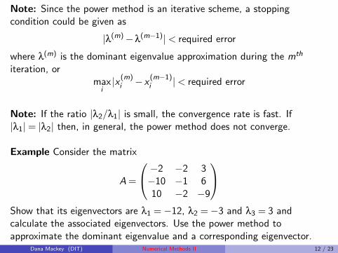
Note: Since the power method is an iterative scheme, a stoppingcondition could be given as

|λ(m)−λ(m−1)|< required error

where λ(m) is the dominant eigenvalue approximation during the mth

iteration, ormax

i|x (m)

i −x(m−1)i |< required error

Note: If the ratio |λ2/λ1| is small, the convergence rate is fast. If|λ1|= |λ2| then, in general, the power method does not converge.

Example Consider the matrix

A =

−2 −2 3−10 −1 610 −2 −9

Show that its eigenvectors are λ1 =−12, λ2 =−3 and λ3 = 3 andcalculate the associated eigenvectors. Use the power method toapproximate the dominant eigenvalue and a corresponding eigenvector.


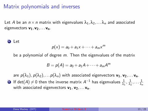
Matrix polynomials and inverses

Let A be an n×n matrix with eigenvalues λ1,λ2, . . .λn and associatedeigenvectors v1,v2, . . .vn.

1 Letp(x) = a0 +a1x + · · ·+amx

m

be a polynomial of degree m. Then the eigenvalues of the matrix

B = p(A) = a0 +a1A+ · · ·+amAm

are p(λ1), p(λ2), . . .p(λn) with associated eigenvectors v1, v2, . . .vn.

2 If det(A) 6= 0 then the inverse matrix A−1 has eigenvalues 1λ1, 1

λ2, . . . 1

λn

with associated eigenvectors v1, v2, . . .vn.


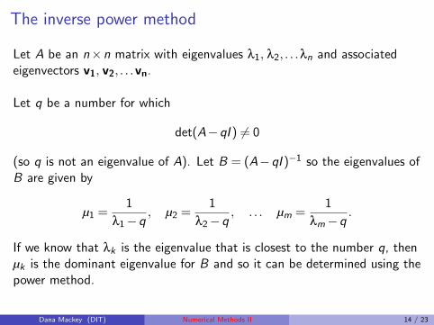
The inverse power method

Let A be an n×n matrix with eigenvalues λ1, λ2, . . .λn and associatedeigenvectors v1, v2, . . .vn.

Let q be a number for which

det(A−qI ) 6= 0

(so q is not an eigenvalue of A). Let B = (A−qI )−1 so the eigenvalues ofB are given by

µ1 =1

λ1−q, µ2 =

1

λ2−q, . . . µm =

1

λm−q.

If we know that λk is the eigenvalue that is closest to the number q, thenµk is the dominant eigenvalue for B and so it can be determined using thepower method.


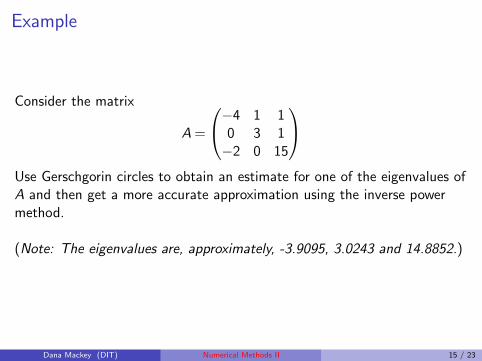
Example

Consider the matrix

A =

−4 1 10 3 1−2 0 15

Use Gerschgorin circles to obtain an estimate for one of the eigenvalues ofA and then get a more accurate approximation using the inverse powermethod.

(Note: The eigenvalues are, approximately, -3.9095, 3.0243 and 14.8852.)


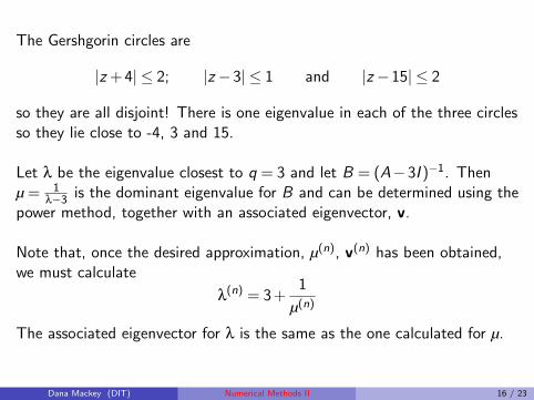
The Gershgorin circles are

|z + 4| ≤ 2; |z−3| ≤ 1 and |z−15| ≤ 2

so they are all disjoint! There is one eigenvalue in each of the three circlesso they lie close to -4, 3 and 15.

Let λ be the eigenvalue closest to q = 3 and let B = (A−3I )−1. Thenµ = 1

λ−3 is the dominant eigenvalue for B and can be determined using thepower method, together with an associated eigenvector, v.

Note that, once the desired approximation, µ(n), v(n) has been obtained,we must calculate

λ(n) = 3 +

1

µ(n)

The associated eigenvector for λ is the same as the one calculated for µ.


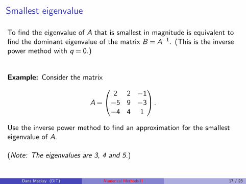
Smallest eigenvalue

To find the eigenvalue of A that is smallest in magnitude is equivalent tofind the dominant eigenvalue of the matrix B = A−1. (This is the inversepower method with q = 0.)

Example: Consider the matrix

A =

2 2 −1−5 9 −3−4 4 1

.

Use the inverse power method to find an approximation for the smallesteigenvalue of A.

(Note: The eigenvalues are 3, 4 and 5.)


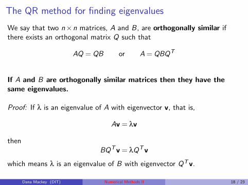
The QR method for finding eigenvalues

We say that two n×n matrices, A and B, are orthogonally similar ifthere exists an orthogonal matrix Q such that

AQ = QB or A = QBQT

If A and B are orthogonally similar matrices then they have thesame eigenvalues.

Proof: If λ is an eigenvalue of A with eigenvector v, that is,

Av = λv

thenBQTv = λQTv

which means λ is an eigenvalue of B with eigenvector QTv.


To find the eigenvalues of a matrix A using the QR algorithm, we generatea sequence of matrices A(m) which are orthogonally similar to A (and sohave the same eigenvalues), and which converge to a matrix whoseeigenvalues are easily found.

If the matrix A is symmetric and tridiagonal then the sequence of QRiterations converges to a diagonal matrix, so its eigenvalues can easily beread from the main diagonal.


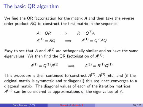
The basic QR algorithm

We find the QR factorisation for the matrix A and then take the reverseorder product RQ to construct the first matrix in the sequence.

A = QR =⇒ R = QTA

A(1) = RQ =⇒ A(1) = QTAQ

Easy to see that A and A(1) are orthogonally similar and so have the sameeigenvalues. We then find the QR factorisation of A(1):

A(1) = Q(1)R(1) =⇒ A(2) = R(1)Q(1)

This procedure is then continued to construct A(2), A(3), etc. and (if theoriginal matrix is symmetric and tridiagonal) this sequence converges to adiagonal matrix. The diagonal values of each of the iteration matricesA(m) can be considered as approximations of the eigenvalues of A.


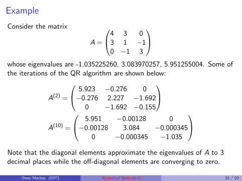
Example

Consider the matrix

A =

4 3 03 1 −10 −1 3

whose eigenvalues are -1.035225260, 3.083970257, 5.951255004. Some ofthe iterations of the QR algorithm are shown below:

A(2) =

5.923 −0.276 0−0.276 2.227 −1.692

0 −1.692 −0.155

A(10) =

5.951 −0.00128 0−0.00128 3.084 −0.000345

0 −0.000345 −1.035

Note that the diagonal elements approximate the eigenvalues of A to 3decimal places while the off-diagonal elements are converging to zero.


Remarks

1 Since the rate of convergence of the QR algorithm is quite slow(especially when the eigenvalues are closely spaced in magnitude)there are a number of variations of this algorithm (not discussed here)which can accelerate convergence.

2 The QR algorithm can be used for finding eigenvectors as well but wewill not cover this technique now

Exercise: Calculate the first iteration of the QR algorithm for the matrixon the previous slide.


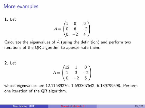
More examples

1. Let

A =

1 0 00 6 −20 −2 4

Calculate the eigenvalues of A (using the definition) and perform twoiterations of the QR algorithm to approximate them.

2. Let

A =

12 1 01 3 −20 −2 5

whose eigenvalues are 12.11689276, 1.693307642, 6.189799598. Performone iteration of the QR algorithm.


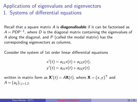
Applications of eigenvalues and eigenvectors1. Systems of differential equations

Recall that a square matrix A is diagonalisable if it can be factorised asA = PDP−1, where D is the diagonal matrix containing the eigenvalues ofA along the diagonal, and P (called the modal matrix) has thecorresponding eigenvectors as columns.

Consider the system of 1st order linear differential equations

x ′(t) = a11x(t) +a12y(t),

y ′(t) = a21x(t) +a22y(t)

written in matrix form as X′(t) = AX(t), where X = (x ,y)T andA = (aij)i .j=1,2.


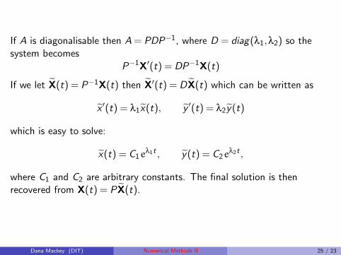
If A is diagonalisable then A = PDP−1, where D = diag(λ1,λ2) so thesystem becomes

P−1X′(t) = DP−1X(t)

If we let X(t) = P−1X(t) then X′(t) = DX(t) which can be written as

x ′(t) = λ1x(t), y ′(t) = λ2y(t)

which is easy to solve:

x(t) = C1 eλ1t , y(t) = C2 eλ2t ,

where C1 and C2 are arbitrary constants. The final solution is thenrecovered from X(t) = PX(t).


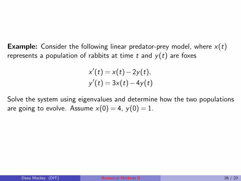
Example: Consider the following linear predator-prey model, where x(t)represents a population of rabbits at time t and y(t) are foxes

x ′(t) = x(t)−2y(t),

y ′(t) = 3x(t)−4y(t)

Solve the system using eigenvalues and determine how the two populationsare going to evolve. Assume x(0) = 4, y(0) = 1.


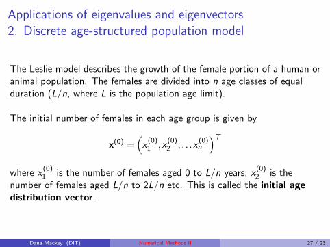
Applications of eigenvalues and eigenvectors2. Discrete age-structured population model

The Leslie model describes the growth of the female portion of a human oranimal population. The females are divided into n age classes of equalduration (L/n, where L is the population age limit).

The initial number of females in each age group is given by

x(0) =(x(0)1 ,x

(0)2 , . . .x

(0)n

)Twhere x

(0)1 is the number of females aged 0 to L/n years, x

(0)2 is the

number of females aged L/n to 2L/n etc. This is called the initial agedistribution vector.


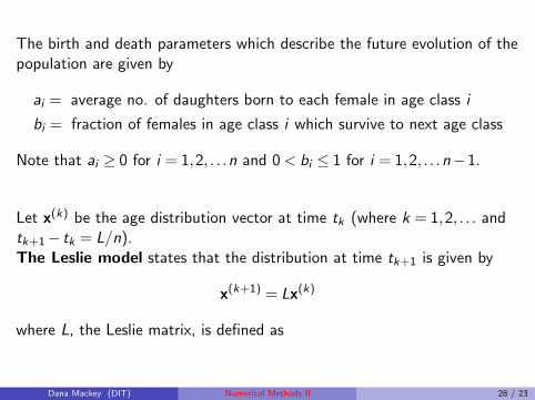
The birth and death parameters which describe the future evolution of thepopulation are given by

ai = average no. of daughters born to each female in age class i

bi = fraction of females in age class i which survive to next age class

Note that ai ≥ 0 for i = 1,2, . . .n and 0 < bi ≤ 1 for i = 1,2, . . .n−1.

Let x(k) be the age distribution vector at time tk (where k = 1,2, . . . andtk+1− tk = L/n).The Leslie model states that the distribution at time tk+1 is given by

x(k+1) = Lx(k)

where L, the Leslie matrix, is defined as


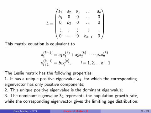
L =

a1 a2 a3 . . . anb1 0 0 . . . 00 b2 0 . . . 0...

......

......

0 . . . 0 bn−1 0

This matrix equation is equivalent to

x(k+1)1 = a1x

(k)1 +a2x

(k)2 + · · ·anx

(k)n

x(k+1)i+1 = bix

(k)i , i = 1,2, . . .n−1

The Leslie matrix has the following properties:1. It has a unique positive eigenvalue λ1, for which the correspondingeigenvector has only positive components;2. This unique positive eigenvalue is the dominant eigenvalue;3. The dominant eigenvalue λ1 represents the population growth rate,while the corresponding eigenvector gives the limiting age distribution.


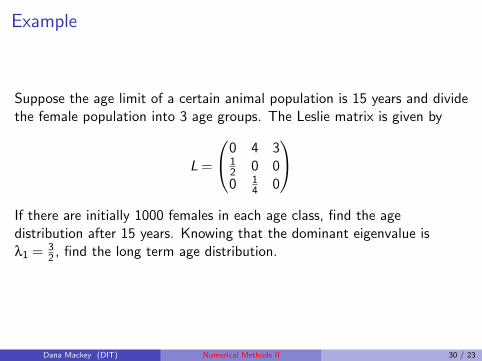
Example

Suppose the age limit of a certain animal population is 15 years and dividethe female population into 3 age groups. The Leslie matrix is given by

L =

0 4 312 0 00 1

4 0

If there are initially 1000 females in each age class, find the agedistribution after 15 years. Knowing that the dominant eigenvalue isλ1 = 3

2 , find the long term age distribution.


Eigenvalues and eigenvectors of a matrix - Dublin …dmackey/lectures/Eigenvals.pdfEigenvalues and...

Documents

Transcript of Eigenvalues and eigenvectors of a matrix - Dublin …dmackey/lectures/Eigenvals.pdfEigenvalues and...