Eigenvalues and Eigenvectors - Peoplepeople.sc.fsu.edu/~jpeterson/Eigen.pdf · Eigenvalues and...
82
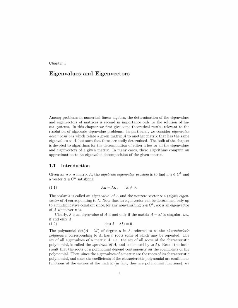
Chapter 1 Eigenvalues and Eigenvectors Among problems in numerical linear algebra, the determination of the eigenvalues and eigenvectors of matrices is second in importance only to the solution of lin- ear systems. In this chapter we first give some theoretical results relevant to the resolution of algebraic eigenvalue problems. In particular, we consider eigenvalue decompositions which relate a given matrix A to another matrix that has the same eigenvalues as A, but such that these are easily determined. The bulk of the chapter is devoted to algorithms for the determination of either a few or all the eigenvalues and eigenvectors of a given matrix. In many cases, these algorithms compute an approximation to an eigenvalue decomposition of the given matrix. 1.1 Introduction Given an n × n matrix A, the algebraic eigenvalue problem is to find a λ ∈ C k and a vector x ∈ C n satisfying Ax = λx , x =0 . (1.1) The scalar λ is called an eigenvalue of A and the nonzero vector x a(right) eigen- vector of A corresponding to λ. Note that an eigenvector can be determined only up to a multiplicative constant since, for any nonvanishing α ∈ C k , αx is an eigenvector of A whenever x is. Clearly, λ is an eigenvalue of A if and only if the matrix A - λI is singular, i.e., if and only if det(A - λI )=0 . (1.2) The polynomial det(A - λI ) of degree n in λ, referred to as the characteristic polynomial corresponding to A, has n roots some of which may be repeated. The set of all eigenvalues of a matrix A, i.e., the set of all roots of the characteristic polynomial, is called the spectrum of A, and is denoted by λ(A). Recall the basic result that the roots of a polynomial depend continuously on the coefficients of the polynomial. Then, since the eigenvalues of a matrix are the roots of its characteristic polynomial, and since the coefficients of the characteristic polynomial are continuous functions of the entries of the matrix (in fact, they are polynomial functions), we 1
Transcript of Eigenvalues and Eigenvectors - Peoplepeople.sc.fsu.edu/~jpeterson/Eigen.pdf · Eigenvalues and...
Chapter 1
Eigenvalues and Eigenvectors
Among problems in numerical linear algebra, the determination of the eigenvaluesand eigenvectors of matrices is second in importance only to the solution of lin-ear systems. In this chapter we first give some theoretical results relevant to theresolution of algebraic eigenvalue problems. In particular, we consider eigenvaluedecompositions which relate a given matrix A to another matrix that has the sameeigenvalues as A, but such that these are easily determined. The bulk of the chapteris devoted to algorithms for the determination of either a few or all the eigenvaluesand eigenvectors of a given matrix. In many cases, these algorithms compute anapproximation to an eigenvalue decomposition of the given matrix.
1.1 Introduction
Given an n× n matrix A, the algebraic eigenvalue problem is to find a λ ∈ Ck anda vector x ∈ Cn satisfying
Ax = λx , x 6= 0 .(1.1)
The scalar λ is called an eigenvalue of A and the nonzero vector x a (right) eigen-vector of A corresponding to λ. Note that an eigenvector can be determined only upto a multiplicative constant since, for any nonvanishing α ∈ Ck, αx is an eigenvectorof A whenever x is.
Clearly, λ is an eigenvalue of A if and only if the matrix A− λI is singular, i.e.,if and only if
det(A− λI) = 0 .(1.2)
The polynomial det(A − λI) of degree n in λ, referred to as the characteristicpolynomial corresponding to A, has n roots some of which may be repeated. Theset of all eigenvalues of a matrix A, i.e., the set of all roots of the characteristicpolynomial, is called the spectrum of A, and is denoted by λ(A). Recall the basicresult that the roots of a polynomial depend continuously on the coefficients of thepolynomial. Then, since the eigenvalues of a matrix are the roots of its characteristicpolynomial, and since the coefficients of the characteristic polynomial are continuousfunctions of the entries of the matrix (in fact, they are polynomial functions), we
1
2 1. Eigenvalues and Eigenvectors
can conclude that the eigenvalues of a matrix depend continuously on the entriesof the matrix.
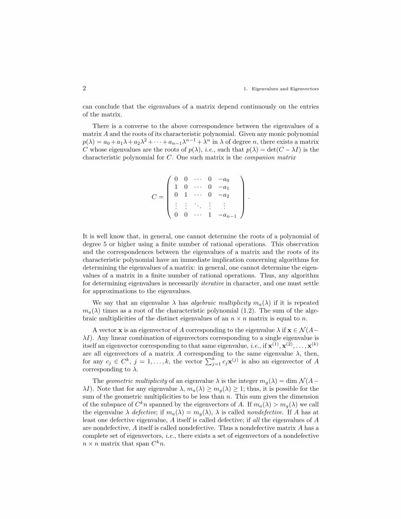
There is a converse to the above correspondence between the eigenvalues of amatrix A and the roots of its characteristic polynomial. Given any monic polynomialp(λ) = a0 +a1λ+a2λ
2 + · · ·+an−1λn−1 +λn in λ of degree n, there exists a matrix
C whose eigenvalues are the roots of p(λ), i.e., such that p(λ) = det(C − λI) is thecharacteristic polynomial for C. One such matrix is the companion matrix
C =
0 0 · · · 0 −a0
1 0 · · · 0 −a1
0 1 · · · 0 −a2
......
. . ....
...0 0 · · · 1 −an−1
.
It is well know that, in general, one cannot determine the roots of a polynomial ofdegree 5 or higher using a finite number of rational operations. This observationand the correspondences between the eigenvalues of a matrix and the roots of itscharacteristic polynomial have an immediate implication concerning algorithms fordetermining the eigenvalues of a matrix: in general, one cannot determine the eigen-values of a matrix in a finite number of rational operations. Thus, any algorithmfor determining eigenvalues is necessarily iterative in character, and one must settlefor approximations to the eigenvalues.
We say that an eigenvalue λ has algebraic multiplicity ma(λ) if it is repeatedma(λ) times as a root of the characteristic polynomial (1.2). The sum of the alge-braic multiplicities of the distinct eigenvalues of an n× n matrix is equal to n.
A vector x is an eigenvector of A corresponding to the eigenvalue λ if x ∈ N (A−λI). Any linear combination of eigenvectors corresponding to a single eigenvalue isitself an eigenvector corresponding to that same eigenvalue, i.e., if x(1),x(2), . . . ,x(k)
are all eigenvectors of a matrix A corresponding to the same eigenvalue λ, then,for any cj ∈ Ck, j = 1, . . . , k, the vector
∑kj=1 cjx(j) is also an eigenvector of A
corresponding to λ.
The geometric multiplicity of an eigenvalue λ is the integer mg(λ) = dim N (A−λI). Note that for any eigenvalue λ, ma(λ) ≥ mg(λ) ≥ 1; thus, it is possible for thesum of the geometric multiplicities to be less than n. This sum gives the dimensionof the subspace of Ckn spanned by the eigenvectors of A. If ma(λ) > mg(λ) we callthe eigenvalue λ defective; if ma(λ) = mg(λ), λ is called nondefective. If A has atleast one defective eigenvalue, A itself is called defective; if all the eigenvalues of Aare nondefective, A itself is called nondefective. Thus a nondefective matrix A has acomplete set of eigenvectors, i.e., there exists a set of eigenvectors of a nondefectiven× n matrix that span Ckn.
1.1. Introduction 3
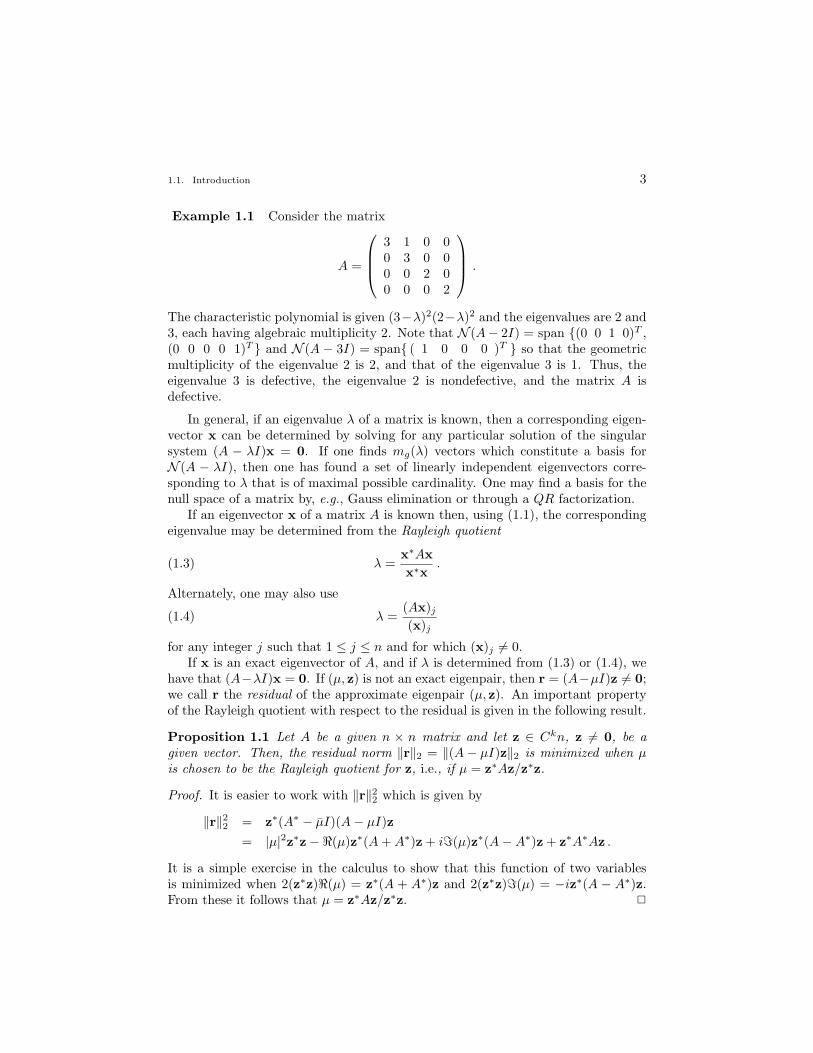
Example 1.1 Consider the matrix
A =
3 1 0 00 3 0 00 0 2 00 0 0 2
.
The characteristic polynomial is given (3−λ)2(2−λ)2 and the eigenvalues are 2 and3, each having algebraic multiplicity 2. Note that N (A− 2I) = span {(0 0 1 0)T ,(0 0 0 0 1)T } and N (A − 3I) = span{ ( 1 0 0 0 )T } so that the geometricmultiplicity of the eigenvalue 2 is 2, and that of the eigenvalue 3 is 1. Thus, theeigenvalue 3 is defective, the eigenvalue 2 is nondefective, and the matrix A isdefective.
In general, if an eigenvalue λ of a matrix is known, then a corresponding eigen-vector x can be determined by solving for any particular solution of the singularsystem (A − λI)x = 0. If one finds mg(λ) vectors which constitute a basis forN (A − λI), then one has found a set of linearly independent eigenvectors corre-sponding to λ that is of maximal possible cardinality. One may find a basis for thenull space of a matrix by, e.g., Gauss elimination or through a QR factorization.
If an eigenvector x of a matrix A is known then, using (1.1), the correspondingeigenvalue may be determined from the Rayleigh quotient
λ =x∗Axx∗x
.(1.3)
Alternately, one may also use
λ =(Ax)j
(x)j(1.4)
for any integer j such that 1 ≤ j ≤ n and for which (x)j 6= 0.If x is an exact eigenvector of A, and if λ is determined from (1.3) or (1.4), we
have that (A−λI)x = 0. If (µ, z) is not an exact eigenpair, then r = (A−µI)z 6= 0;we call r the residual of the approximate eigenpair (µ, z). An important propertyof the Rayleigh quotient with respect to the residual is given in the following result.
Proposition 1.1 Let A be a given n × n matrix and let z ∈ Ckn, z 6= 0, be agiven vector. Then, the residual norm ‖r‖2 = ‖(A− µI)z‖2 is minimized when µis chosen to be the Rayleigh quotient for z, i.e., if µ = z∗Az/z∗z.
Proof. It is easier to work with ‖r‖22 which is given by
‖r‖22 = z∗(A∗ − µI)(A− µI)z= |µ|2z∗z−<(µ)z∗(A + A∗)z + i=(µ)z∗(A−A∗)z + z∗A∗Az .
It is a simple exercise in the calculus to show that this function of two variablesis minimized when 2(z∗z)<(µ) = z∗(A + A∗)z and 2(z∗z)=(µ) = −iz∗(A − A∗)z.From these it follows that µ = z∗Az/z∗z. 2
4 1. Eigenvalues and Eigenvectors
We say that a subspace S is invariant for a matrix A if x ∈ S implies thatAx ∈ S. If S = span{p(1),p(2), . . . ,p(s) } is an invariant subspace for an n × nmatrix A, then there exists an s × s matrix B such that AP = PB, where thecolumns of the n × s matrix P are the vectors p(j), j = 1, . . . , s. Trivially, thespace spanned by n linearly independent vectors belonging to Ckn is an invariantsubspace for any n × n matrix; in this case, the relation between the matrices A,B, and P is given a special name.
Let A and B be n × n matrices. Then A and B are said to be similar if thereexists an invertible matrix P , i.e., a matrix with linearly independent columns, suchthat
B = P−1AP .(1.5)
The relation (1.5) itself is called a similarity transformation. B is said to be unitarilysimilar to A if P is unitary, i.e., if B = P ∗AP and P ∗P = I.
The following proposition shows that similar matrices have the same character-istic polynomial and thus the same set of eigenvalues having the same algebraicmultiplicities; the geometric multiplicites of the eigenvalues are also unchanged.
Proposition 1.2 Let A be an n × n matrix and P an n × n nonsingular matrix.Let B = P−1AP . If λ is an eigenvalue of A of algebraic (geometric) multiplicityma (mg), then λ is an eigenvalue of B of algebraic (geometric) multiplicity ma
(mg). Moreover, if x is an eigenvector of A corresponding to λ then P−1x is aneigenvector of B corresponding to the same eigenvalue λ.
Proof. Since Ax = λx and P is invertible, we have that
P−1AP (P−1x) = λP−1x
so that if (λ,x) is an eigenpair of A then (λ, P−1x) is an eigenpair of B. Todemonstrate that the algebraic multiplicities are unchanged after a similarity trans-formation, we show that A and B have the same characteristic polynomial. Indeed,
det(B − λI) = det(P−1AP − λI) = det(P−1(A− λI)P )= det(P−1) det(A− λI) detP = det(A− λI) .
That the geometric multiplicities are also unchanged follows from
0 = (A− λI)x = P (B − λI)(P−1x)
and the invertibility of P . 2
It is easily seen that any set consisting of eigenvectors of a matrix A is an invari-ant set for A. In particular, the eigenvectors corresponding to a single eigenvalue λform an invariant set. Since linear combinations of eigenvectors corresponding to asingle eigenvalue are also eigenvectors, it is often the case that these invariant setsare of more interest than the individual eigenvectors.
1.1. Introduction 5
If an n × n matrix is defective, the set of eigenvectors does not span Cn. Infact, the cardinality of any set of linearly independent eigenvectors is necessarilyless than or equal to the sum of the geometric multiplicities of the eigenvalues ofA. Corresponding to any defective eigenvalue λ of a matrix A, one may definegeneralized eigenvectors that satisfy, instead of (1.1),
Ay = λy + z ,(1.6)
where z is either an eigenvector or another generalized eigenvector of A. The num-ber of linearly independent generalized eigenvectors corresponding to a defectiveeigenvalue λ is given by ma(λ) − mg(λ), so that the total number of generalizedeigenvectors of a defective n × n matrix A is n − k, where k =
∑Kj=1 mg(λj) and
λj , j = 1, . . . ,K, denote the distinct eigenvalues of A. The set of eigenvectors andgeneralized eigenvectors corresponding to the same eigenvalue form an invariantsubset. The set of all eigenvectors and generalized eigenvectors of an n× n matrixA do span Cn. Moreover, there always exists a set consisting of k eigenvectors andn− k generalized eigenvectors which forms a basis for Cn.
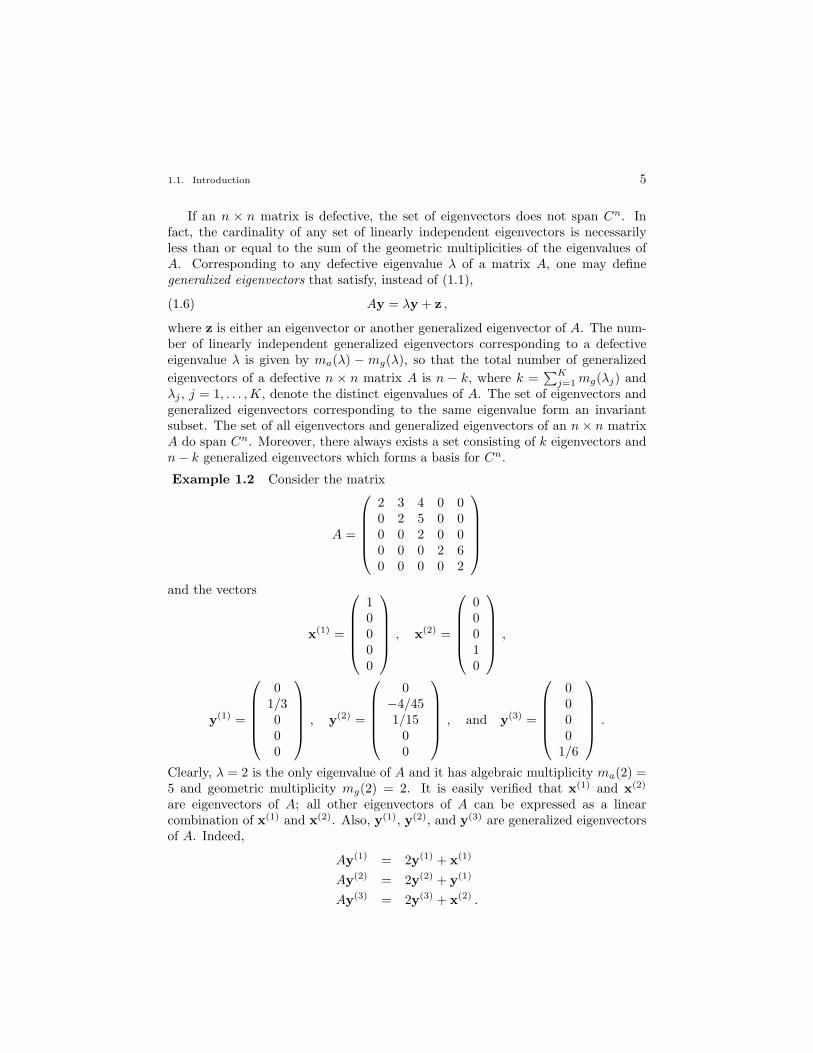
Example 1.2 Consider the matrix
A =
2 3 4 0 00 2 5 0 00 0 2 0 00 0 0 2 60 0 0 0 2
and the vectors
x(1) =
10000
, x(2) =
00010
,
y(1) =
0
1/3000
, y(2) =
0
−4/451/15
00
, and y(3) =
0000
1/6
.
Clearly, λ = 2 is the only eigenvalue of A and it has algebraic multiplicity ma(2) =5 and geometric multiplicity mg(2) = 2. It is easily verified that x(1) and x(2)
are eigenvectors of A; all other eigenvectors of A can be expressed as a linearcombination of x(1) and x(2). Also, y(1), y(2), and y(3) are generalized eigenvectorsof A. Indeed,
Ay(1) = 2y(1) + x(1)
Ay(2) = 2y(2) + y(1)
Ay(3) = 2y(3) + x(2) .
6 1. Eigenvalues and Eigenvectors
Finally, the set {x(1) , x(2) , y(1) , y(2) , y(3) } spans RI 5.
The precise nature of the relations between eigenvectors and generalized eigen-vectors of a matrix A may be determined from its Jordan canonical form which wedo not discuss here.
If U is an upper triangular matrix, its eigenvalues and eigenvectors are easilydetermined, i.e., the eigenvalues are the diagonal entries of U and the eigenvectorsmay be found through a simple back substitution process. Also, if A is a block uppertriangular matrix, i.e., a matrix of the form
A =
A11 A12 A13 · · · A1m
0 A22 A23 · · · A2m
0 0 A33 · · · A3m
......
. . ....
0 0 0 · · · Amm
,
where the diagonal blocks Aii, i = 1, . . . ,m, are square, then it is easy todemonstrate that the eigenvalues of A are merely the union of the eigenvalues ofAii for i = 1, . . . ,m.
We close this section by giving a localization theorem for eigenvalues, i.e., aresult which allows us to determine regions in the complex plane that contain theeigenvalues of a given matrix.
Theorem 1.3 (Gerschgorin Circle Theorem) Let A be a given n×n matrix. Definethe disks
Di ={
z ∈ Ck : |ai,i − z| ≤n∑
j=1j 6=i
|ai,j |}
for i = 1, . . . , n .(1.7)
Then every eigenvalue of A lies in the union of the disks S = ∪ni=1Di. Moreover, if
Sk denotes the union of k disks, 1 ≤ k ≤ n, which are disjoint from the remaining(n − k) disks, then Sk contains exactly k eigenvalues of A counted according toalgebraic multiplicity.
Proof. Let (λ,x) be an eigenpair of A and define the index i by |xi| = ‖x‖∞. Since
n∑j=1
ai,jxj − λxi = 0
we have that
|ai,i − λ| |xi| = |ai,ixi − λxi| =∣∣∣ n∑j=1j 6=i
ai,jxj
∣∣∣ ≤ n∑j=1j 6=i
|ai,j | |xi|
1.2. Eigenvalue Decompositions 7
and since x 6= 0, we have that xi 6= 0 and therefore (1.7) holds.For the second result, let
A = D + B and for i = 1, . . . , n, si =n∑
j=1j 6=i
|ai,j | ,
where D is the diagonal of A. Now, for 0 ≤ t ≤ 1, consider the matrix C = D + tB.Since the eigenvalues of C are continuous functions of t, as t varies from 0 to 1 eachof these eigenvalues describes a continuous curve in the complex plane. Also, bythe first result of the theorem, for any t, the eigenvalues of C lie in the union of thedisks centered at ai and of radii tsi ≤ si. Note that since t ∈ [0, 1], each disk ofradius tsi is contained within the disk of radius si. Without loss of generality wemay assume that it is the first k disks that are disjoint from the remaining (n− k)disks so that the disks with radii sk+1, . . . , sn are isolated from Sk = ∪k
i=1Di. Thisremains valid for all t ∈ [0, 1], i.e., the disks with radii tsk+1, . . . , tsn are isolatedfrom those with radii ts1, . . . , tsk. Now, when t = 0, the eigenvalues of C are givenby a1,1, . . . , an,n and the first k of these are in Sk and the last (n − k) lie outsideof Sk. Since the eigenvalues describe continuous curves, this remains valid for allt ∈ [0, 1], including t = 1 for which C = A. 2
Example 1.3 The matrix A given by
A =
2 0 11 −3 −1−1 1 4
has eigenvalues −
√8,√
8, and 3. All the eigenvalues of A lie in D1 ∪ D2 ∪ D3,where
D1 = {z ∈ CI 1 : |z− 2| ≤ 1}D2 = {z ∈ CI 1 : |z + 3| ≤ 2}D3 = {z ∈ CI 1 : |z− 4| ≤ 2} .
Moreover, since D2 is disjoint from D1 ∪ D3 we have that exactly one eigenvaluelies in D2 and two eigenvalues lie in D1 ∪D3.
1.2 Eigenvalue Decompositions
In this section we show that a given n × n matrix is similar to a matrix whoseeigenvalues and eigenvectors are easily determined. The associated similarity trans-formations are referred to as eigenvalue decompositions. We will examine severalsuch decompositions, beginning with the central result in this genre, which is knownas the Schur decomposition.
8 1. Eigenvalues and Eigenvectors
Theorem 1.4 Let A be a given n× n matrix. Then there exists an n× n unitarymatrix Q such that
Q∗AQ = U ,(1.8)
where U is an upper triangular matrix whose diagonal entries are the eigenvalues ofA. Furthermore, Q can be chosen so that the eigenvalues of A appear in any orderalong the diagonal of U .
Proof. The proof is by induction on n. For n = 1 the proof is trivial since A isa scalar in this case. Now assume that for any (n − 1) × (n − 1) matrix B thereexists an (n− 1)× (n− 1) unitary matrix Q such that Q∗BQ is upper triangular.Let (λ1,x(1)) be an eigenpair of A, i.e., Ax(1) = λ1x(1); normalize x(1) so that‖x(1)‖2 = 1. Now x(1) ∈ Cn so there exists an orthonormal basis for Cn whichcontains the vector x(1); denote this basis set by {x(1),x(2), . . . ,x(n)} and let X bethe n × n unitary matrix whose j-th column is the vector x(j). Now, due to theorthonormality of the columns of X, X∗AX can be partitioned in the form
X∗AX =(
λ1 y∗
0 B
),
where y is an (n − 1)−vector and B is an (n − 1) × (n − 1) matrix. From theinduction hypothesis there exists a unitary matrix Q such that Q∗BQ is uppertriangular. Choose
Q = X
(1 00 Q
);
note that Q is a unitary matrix. Then
Q∗AQ =(
1 00 Q∗
)X∗AX
(1 00 Q
)=
(1 00 Q∗
)(λ1 y∗
0 B
)(1 00 Q
)=
(λ1 y∗Q0 Q∗BQ
),
where the last matrix is an upper triangular matrix since Q∗BQ is upper triangular.Thus A is unitarily similar to the upper triangular matrix U = Q∗AQ and thereforeU and A have the same eigenvalues which are given by the diagonal entries ofU . Also, since λ1 can be any eigenvalue of A, it is clear that we may chooseany ordering for the appearance of the eigenvalues along the diagonal of the uppertriangular matrix U . 2
Given a matrix A, suppose that its Schur decomposition is known, i.e., U andQ in (1.8) are known. Then, since the eigenvalues of A and U are the same, theeigenvalues of the former are determined. Furthermore, if y is an eigenvector of Ucorresponding to an eigenvalue λ, then x = Qy is an eigenvector of A corresponding
1.2. Eigenvalue Decompositions 9
to the same eigenvalue, so that the eigenvectors of A are also easily determined fromthose of U .
In many cases where a matrix has some special characteristic, more informationabout the structure of the Schur decomposition can be established. Before exam-ining one such consequence of the Schur decomposition, we consider the possibilityof a matrix being similar to diagonal matrix.
An n× n matrix A is diagonalizable if there exists a nonsingular matrix P anda diagonal matrix Λ such that
P−1AP = Λ ,(1.9)
i.e., if A is similar to a diagonal matrix.From Proposition 1.2 it is clear that if A is diagonalizable, then the entries
of the diagonal matrix Λ are the eigenvalues of A. Also, P−1AP = Λ impliesthat AP = PΛ so that the columns of P are eigenvectors of A. To see this, letλ1, λ2, . . . , λn denote the eigenvalues of A, let Λ = diag(λ1, λ2, . . . , λn), and let p(j)
denote the j-th column of P , then Ap(j) = λjp(j), i.e., p(j) is an eigenvector of Acorresponding to the eigenvalue λj .
Not all matrices are diagonalizable, as is shown in the following result.
Proposition 1.5 Let A be an n× n matrix. Then A is diagonalizable if and onlyif A is nondefective.
Proof. Assume that A is diagonalizable. Then there exists an invertible matix Psuch that P−1AP = Λ, where Λ is a diagonal matrix. As was indicated above, thecolumns of P are eigenvectors of A, and since P is invertible, these eigenvectorsform an n-dimensional linearly independent set, i.e., a basis for Ckn. Thus A isnondefective.
Now assume that A is nondefective, i.e., A has a complete set of linearly in-dependent eigenvectors which form a basis for Cn. Denote these vectors by p(j),j = 1, . . . , n, and define the n× n matrix P to be the matrix whose j-th column isp(j). Then
AP = PΛ ,
where Λ = diag (λ1, λ2, . . . , λn). Since P is invertible we have that
P−1AP = Λ
and thus A is diagonalizable. 2
Some matrices are unitarily diagonalizable, i.e., P in (1.9) is a unitary matrix.From another point of view, for these matrices, the upper triangular matrix U in(1.8) is a diagonal matrix. Recall that an n× n matrix A is normal if AA∗ = A∗A.All unitary, Hermitian, and skew-Hermitian matrices are normal. We now showthat a matrix is normal if and only if it is unitarily diagonalizable.
10 1. Eigenvalues and Eigenvectors
Proposition 1.6 Let A be an n×n matrix. Then A is normal if and only if thereexists a unitary matrix Q such that Q∗AQ is diagonal. Moreover, the columns of Qare eigenvectors of A so that normal matrices have a complete, orthonormal set oflinearly independent eigenvectors; in particular, normal matrices are nondefective.
Proof. Let A be a normal matrix. From Theorem 1.4 A is unitarily similar to anupper triangular matrix U , i.e., Q∗AQ = U where Q∗Q = I. But, since A is normal,so is U , i.e.,
UU∗ = Q∗AQQ∗A∗Q = Q∗AA∗Q = Q∗A∗AQ = Q∗A∗QQ∗AQ = U∗U .
By equating entries of UU∗ and U∗U we can show that a normal upper triangularmatrix must be diagonal.
We now show that if A is unitarily diagonalizable, then it is normal. Let Q bea unitary matrix such that
Q∗AQ = Λ ,
where Λ is a diagonal matrix. Then A is normal since
AA∗ = QΛQ∗QΛ∗Q∗ = QΛΛ∗Q∗ = QΛ∗ΛQ∗ = QΛ∗Q∗QΛQ∗ = A∗A ,
where we have used the fact that diagonal matrices commute.From Q∗AQ = Λ, we have that AQ = QΛ, so that if Λ = diag(λ1, λ2, . . . , λn)
and q(j) denotes the j-th column of Q, then Aq(j) = λjq(j), i.e., q(j) is an eigen-vector of A corresponding to the eigenvalue λj . 2
Corollary 1.7 Let A be an n × n Hermitian matrix. Then there exists a unitarymatrix Q such that Q∗AQ is a real diagonal matrix. Moreover, the columns of Qare eigenvectors of A and thus Hermitian matrices are nondefective and possess acomplete, orthonormal set of eigenvectors.
Proof. Let Q∗AQ = U be the Schur decomposition of A, where A is Hermitian.Then U is also Hermitian, i.e., U∗ = Q∗A∗Q = Q∗AQ = U . But U is also anupper triangular matrix so that it easily follows that U is a diagonal matrix andthat its diagonal entries are real. Again, as in Proposition 1.6, the columns of Qare eigenvectors of A. 2
If A is a real, symmetric matrix, then Q may be chosen to be real as well inwhich case Q is an orthogonal matrix. Thus, symmetric matrices possess a complete,orthonormal set of real eigenvectors.
Example 1.4 Let A be the symmetric matrix
A =
−2 0 −360 −3 0
−36 0 −23
.
1.2. Eigenvalue Decompositions 11
Then A is orthogonally similar to a diagonal matrix, i.e.,
QT AQ =
−4/5 0 3/50 1 0
3/5 0 4/5
−2 0 −360 −3 0
−36 0 −23
−4/5 0 3/50 1 0
3/5 0 4/5
=
25 0 00 −3 00 0 −50
.
If A is a real matrix having complex eigenvalues, then its Schur decompositionnecessarily must involve complex arithmetic, i.e., if one wishes to use only realarithmetic, similarity to an upper triangular matrix cannot be achieved. However,if A is a real matrix, then its characteristic polynomial has real coefficients andtherefore its complex eigenvalues must occur in complex conjugate pairs. The cor-responding eigenvectors may be chosen to occur in complex conjugate pairs as well,i.e., if x + iy is an eigenvector corresponding to an eigenvalue λ, then x− iy is aneigenvector corresponding to λ. (Note that if λ is a complex eigenvalue of a realmatrix A, then its corresponding eigenvectors are necessarily complex, i.e., y 6= 0.On the other hand, if λ is a real eigenvalue of a real matrix, then its correspondingeigenvectors may be chosen to be real.) These observations lead to the followingreal Schur decomposition of a given real matrix A wherein only real arithmetic isneeded and for which A is similar to a quasi-upper triangular matrix.
Proposition 1.8 Let A be an n × n real matrix. Then there exists an orthogonalmatrix Q such that QT AQ is a real matrix of the form
QT AQ =
U1,1 U1,2 · · · U1,m
0 U2,2 · · · U2,m
......
. . ....
0 0 · · · Um,m
,(1.10)
where each Ui,i is either a scalar or is a 2× 2 matrix with complex conjugate eigen-values. The eigenvalues of A are the union of the eigenvalues of Ui,i, i = 1, . . . ,m.
Proof. Let µ denote the number of pairs of eigenvalues occurring as complex con-jugates; clearly, 0 ≤ µ ≤ n/2. If µ = 0, then all the eigenvalues of A are real and allthe eigenvectors may be chosen to be real as well. Then, the proof of Theorem 1.4may be easily amended so that only real arithmetic is utilized; hence in the caseµ = 0, we have that QT AQ = U , where Q is an orthogonal matrix and U is a realupper triangular matrix. Thus, if µ = 0, the decomposition (1.10) is demonstrated.
Now, let µ ≥ 1 so that necessarily n > 1. Clearly the result is true for 0× 0 and1× 1 matrices. Now, assume that the result is true for any (n− 2)× (n− 2) matrixB, i.e., there exists an (n − 2) × (n − 2) orthogonal matrix Q such that QT BQhas the requisite structure. Next, for α, β ∈ RI and x,y ∈ RI n, let (α + iβ,x + iy)
12 1. Eigenvalues and Eigenvectors
and (α − iβ,x − iy) denote a complex conjugate eigenpair of A, i.e., A(x ± iy) =(α± iβ)(x± iy). Then
A (x y ) = (x y ) F where F =(
α β−β α
)(1.11)
so that x and y span an invariant subspace. Furthermore, if β 6= 0, as we aresupposing, the set {x y} is linearly independent since otherwise x + iy = (1 + ci)xfor some real number c so that then x is a real eigenvector corresponding to thecomplex eigenvalue α + iβ of a real matrix; this clearly is impossible. Therefore wemay choose x(1) ∈ RI n and x(2) ∈ RI n to form an orthonormal basis for span{x,y}.Then there exists an invertible 2 × 2 matrix S such that (x y ) = (x(1) x(2) )S.Then, (1.11) implies that
A (x(1) x(2) )S = (x(1) x(2) )SF
or
A( x(1) x(2) ) = (x(1) x(2) )SFS−1 .(1.12)
Now choose x(j) ∈ RI n, j = 3, . . . , n, so that {x(1),x(2), . . . ,x(n)} forms anorthonormal basis for RI n. Let X be the n×n orthogonal matrix whose j-th columnis the vector x(j). Now, due to (1.12) and the orthonormality of the columns of X,XT AX can be partitioned in the form
XT AX =(
SFS−1 Y0 B
),
where Y is a 2 × (n − 1) matrix and B is an (n − 2) × (n − 2) matrix. Fromthe induction hypothesis there exists an orthogonal matrix Q such that QT BQ isquasi-upper triangular. Choose
Q = X
(I2 00 Q
).
Then
QT AQ =(
I2 00 QT
)XT AX
(I2 00 Q
)=
(I2 00 QT
)(SFS−1 Y
0 B
)(I2 00 Q
)=
(SFS−1 Y Q
0 QT BQ
),
where the last matrix is a quasi-upper triangular matrix since QT BQ is quasi-uppertriangular and SFS−1 is a 2× 2 matrix. Thus, the inductive step is complete and
1.3. Reduction to Hessenberg form 13
A is orthogonally similar to a quasi-upper triangular matrix. Of course, A and thematrix QT AQ constructed above have the same eigenvalues since they are relatedthrough a similarity transformation. In fact, the 2 × 2 diagonal block SFS−1 issimilar to F , so that the eigenvalues of SFS−1 are α± iβ. 2
Example 1.5 Let
A =
3/2 −1/2 3/√
21/2 1/2 1/
√2
−1/√
2 1/√
2 1
, Q =
1/√
2 1/√
2 01/√
2 −1/√
2 00 0 1
,
and
U =
1 1 20 1 10 −1 1
.
Then QT Q = I and QT AQ = U . Note that
U11 = 1 , U22 =(
1 1−1 1
)and λ(U11) = 1 and λ(U22) = 1± i; these are the three eigenvalues of A.
1.3 Reduction to Hessenberg form
It was noted in Section 1.1 that in general the eigenvalues and eigenvectors of amatrix cannot be determined using a finite number of rational operations. Onthe other hand, if any of the eigenvalue decompositions considered in Section 1.2are known, then the eigenvalues and eigenvectors can be determined in a finitenumber of arithmetic operations. Thus, necessarily, all the proofs of that sectionare non-constructive. For example, in the proof of the Schur decomposition, i.e.,Theorem 1.4, one assumes that an eigenpair (λ1,x(1)) is known in order to carryout the inductive step.
Given any square matrix A one can determine an upper Hessenberg matrix A0
that is similar to A through the use of a finite number of arithmetic operations.(Recall that an n×n matrix A is in upper Hessenberg form if ai,j = 0 for i > j +1.)Of course, it would still take an infinite number of rational operations to exactlydetermine the eigenvalues and eigenvectors of A0, so that there seems to be littlereason for wanting to compute A0. However, in many cases, iterative algorithms forthe approximate determination of the eigenvalues and eigenvectors of matrices aremore efficient when applied to matrices in Hessenberg form. Thus, given a matrixA, one often first transforms it into a similar upper Hessenberg matrix before oneapplies the iterative method.
One can effect the transformation to Hessenberg form using either unitary orlower triangular matrices. The former is especially useful for symmetric or Hermi-tian matrices since this characteristic can be preserved throughout the reduction
14 1. Eigenvalues and Eigenvectors
process. For unsymmetric and non-Hermitian matrices the latter are in general lesscostly.
1.3.1 Reduction to Hessenberg form using unitary transformations
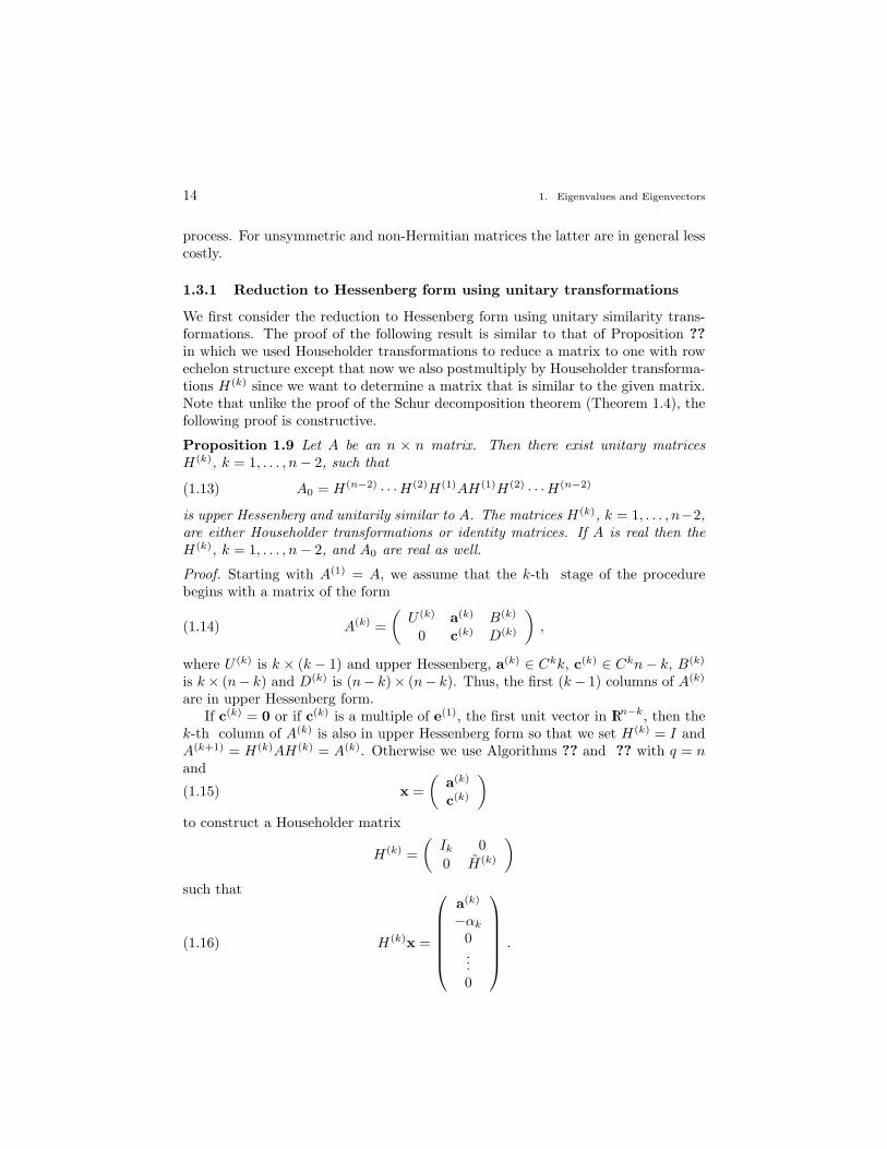
We first consider the reduction to Hessenberg form using unitary similarity trans-formations. The proof of the following result is similar to that of Proposition ??in which we used Householder transformations to reduce a matrix to one with rowechelon structure except that now we also postmultiply by Householder transforma-tions H(k) since we want to determine a matrix that is similar to the given matrix.Note that unlike the proof of the Schur decomposition theorem (Theorem 1.4), thefollowing proof is constructive.
Proposition 1.9 Let A be an n × n matrix. Then there exist unitary matricesH(k), k = 1, . . . , n− 2, such that
A0 = H(n−2) · · ·H(2)H(1)AH(1)H(2) · · ·H(n−2)(1.13)
is upper Hessenberg and unitarily similar to A. The matrices H(k), k = 1, . . . , n−2,are either Householder transformations or identity matrices. If A is real then theH(k), k = 1, . . . , n− 2, and A0 are real as well.
Proof. Starting with A(1) = A, we assume that the k-th stage of the procedurebegins with a matrix of the form
A(k) =(
U (k) a(k) B(k)
0 c(k) D(k)
),(1.14)
where U (k) is k × (k − 1) and upper Hessenberg, a(k) ∈ Ckk, c(k) ∈ Ckn− k, B(k)
is k× (n− k) and D(k) is (n− k)× (n− k). Thus, the first (k− 1) columns of A(k)
are in upper Hessenberg form.If c(k) = 0 or if c(k) is a multiple of e(1), the first unit vector in RI n−k, then the
k-th column of A(k) is also in upper Hessenberg form so that we set H(k) = I andA(k+1) = H(k)AH(k) = A(k). Otherwise we use Algorithms ?? and ?? with q = nand
x =(
a(k)
c(k)
)(1.15)
to construct a Householder matrix
H(k) =(
Ik 00 H(k)
)such that
H(k)x =
a(k)
−αk
0...0
.(1.16)
1.3. Reduction to Hessenberg form 15
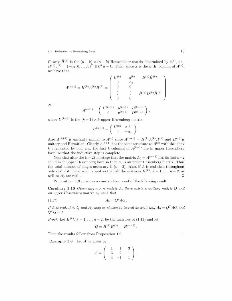
Clearly H(k) is the (n − k) × (n − k) Householder matrix determined by c(k), i.e.,H(k)c(k) = (−αk, 0, . . . , 0)T ∈ Ckn− k. Then, since x is the k-th column of A(k),we have that
A(k+1) = H(k)A(k)H(k) =
U (k) a(k) B(k)H(k)
0 −αk
0 0...
... H(k)D(k)H(k)
0 0
or
A(k+1) =(
U (k+1) a(k+1) B(k+1)
0 c(k+1) D(k+1)
),
where U (k+1) is the (k + 1)× k upper Hessenberg matrix
U (k+1) =(
U (k) a(k)
0 −αk
).
Also A(k+1) is unitarily similar to A(k) since A(k+1) = H(k)A(k)H(k) and H(k) isunitary and Hermitian. Clearly A(k+1) has the same structure as A(k) with the indexk augmented by one, i.e., the first k columns of A(k+1) are in upper Hessenbergform, so that the inductive step is complete.
Note that after the (n−2)-nd stage that the matrix A0 = A(n−1) has its first n−2columns in upper Hessenberg form so that A0 is an upper Hessenberg matrix. Thusthe total number of stages necessary is (n − 2). Also, if A is real then throughoutonly real arithmetic is employed so that all the matrices H(k), k = 1, . . . , n− 2, aswell as A0 are real . 2
Proposition 1.9 provides a constructive proof of the following result.
Corollary 1.10 Given any n × n matrix A, there exists a unitary matrix Q andan upper Hessenberg matrix A0 such that
A0 = Q∗AQ .(1.17)
If A is real, then Q and A0 may be chosen to be real as well, i.e., A0 = QT AQ andQT Q = I.
Proof. Let H(k), k = 1, . . . , n− 2, be the matrices of (1.13) and let
Q = H(1)H(2) · · ·H(n−2) .
Then the results follow from Proposition 1.9. 2
Example 1.6 Let A be given by
A =
1 1 3−3 2 −1
4 −1 1
.
16 1. Eigenvalues and Eigenvectors
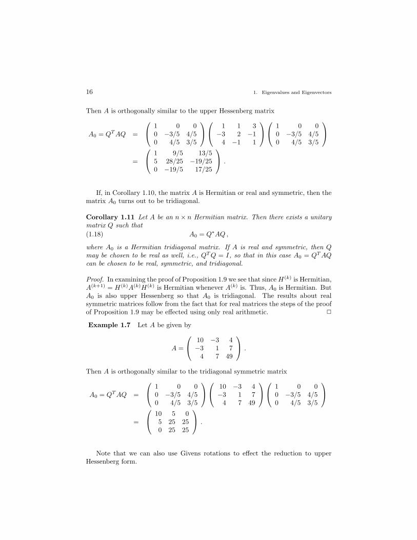
Then A is orthogonally similar to the upper Hessenberg matrix
A0 = QT AQ =
1 0 00 −3/5 4/50 4/5 3/5
1 1 3−3 2 −1
4 −1 1
1 0 00 −3/5 4/50 4/5 3/5
=
1 9/5 13/55 28/25 −19/250 −19/5 17/25
.
If, in Corollary 1.10, the matrix A is Hermitian or real and symmetric, then thematrix A0 turns out to be tridiagonal.
Corollary 1.11 Let A be an n× n Hermitian matrix. Then there exists a unitarymatrix Q such that
A0 = Q∗AQ ,(1.18)
where A0 is a Hermitian tridiagonal matrix. If A is real and symmetric, then Qmay be chosen to be real as well, i.e., QT Q = I, so that in this case A0 = QT AQcan be chosen to be real, symmetric, and tridiagonal.
Proof. In examining the proof of Proposition 1.9 we see that since H(k) is Hermitian,A(k+1) = H(k)A(k)H(k) is Hermitian whenever A(k) is. Thus, A0 is Hermitian. ButA0 is also upper Hessenberg so that A0 is tridiagonal. The results about realsymmetric matrices follow from the fact that for real matrices the steps of the proofof Proposition 1.9 may be effected using only real arithmetic. 2
Example 1.7 Let A be given by
A =
10 −3 4−3 1 7
4 7 49
.
Then A is orthogonally similar to the tridiagonal symmetric matrix
A0 = QT AQ =
1 0 00 −3/5 4/50 4/5 3/5
10 −3 4−3 1 7
4 7 49
1 0 00 −3/5 4/50 4/5 3/5
=
10 5 05 25 250 25 25
.
Note that we can also use Givens rotations to effect the reduction to upperHessenberg form.
1.3. Reduction to Hessenberg form 17
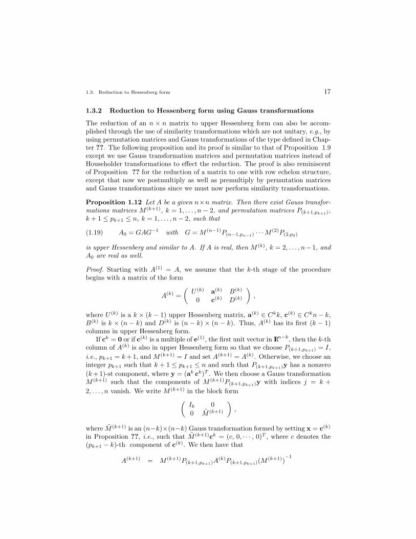
1.3.2 Reduction to Hessenberg form using Gauss transformations
The reduction of an n × n matrix to upper Hessenberg form can also be accom-plished through the use of similarity transformations which are not unitary, e.g., byusing permutation matrices and Gauss transformations of the type defined in Chap-ter ??. The following proposition and its proof is similar to that of Proposition 1.9except we use Gauss transformation matrices and permutation matrices instead ofHouseholder transformations to effect the reduction. The proof is also reminiscentof Proposition ?? for the reduction of a matrix to one with row echelon structure,except that now we postmultiply as well as premultiply by permutation matricesand Gauss transformations since we must now perform similarity transformations.
Proposition 1.12 Let A be a given n×n matrix. Then there exist Gauss transfor-mations matrices M (k+1), k = 1, . . . , n − 2, and permutation matrices P(k+1,pk+1),k + 1 ≤ pk+1 ≤ n, k = 1, . . . , n− 2, such that
A0 = GAG−1 with G = M (n−1)P(n−1,pn−1) · · ·M(2)P(2,p2)(1.19)
is upper Hessenberg and similar to A. If A is real, then M (k), k = 2, . . . , n− 1, andA0 are real as well.
Proof. Starting with A(1) = A, we assume that the k-th stage of the procedurebegins with a matrix of the form
A(k) =(
U (k) a(k) B(k)
0 c(k) D(k)
),
where U (k) is a k × (k − 1) upper Hessenberg matrix, a(k) ∈ Ckk, c(k) ∈ Ckn− k,B(k) is k × (n − k) and D(k) is (n − k) × (n − k). Thus, A(k) has its first (k − 1)columns in upper Hessenberg form.
If ck = 0 or if c(k) is a multiple of e(1), the first unit vector in RI n−k, then the k-thcolumn of A(k) is also in upper Hessenberg form so that we choose P(k+1,pk+1) = I,i.e., pk+1 = k +1, and M (k+1) = I and set A(k+1) = A(k). Otherwise, we choose aninteger pk+1 such that k + 1 ≤ pk+1 ≤ n and such that P(k+1,pk+1)y has a nonzero(k +1)-st component, where y = (ak ck)T . We then choose a Gauss transformationM (k+1) such that the components of M (k+1)P(k+1,pk+1)y with indices j = k +2, . . . , n vanish. We write M (k+1) in the block form(
Ik 00 M (k+1)
),
where M (k+1) is an (n−k)×(n−k) Gauss transformation formed by setting x = c(k)
in Proposition ??, i.e., such that M (k+1)ck = (c, 0, · · · , 0)T , where c denotes the(pk+1 − k)-th component of c(k). We then have that
A(k+1) = M (k+1)P(k+1,pk+1)A(k)P(k+1,pk+1)(M
(k+1))−1
18 1. Eigenvalues and Eigenvectors
=
U (k) a(k) B(k)
0 c0 0...
... M (k+1)D(k)(M (k+1))−1
0 0
,
where B(k) is determined by interchanging the first and (pk+1 − k)-th columnsof B(k) and D(k) is determined by interchanging the first and (pk+1 − k)-th rowand the first and (pk+1 − k)-th columns of D(k). Clearly A(k+1) is similar to A(k)
and has the same structure as A(k) with the index augmented by one, i.e., thefirst k columns of A(k+1) are in upper Hessenberg form. Thus the inductive step iscomplete.
Note that after the (n − 2)-nd stage that the matrix A0 = A(n−1) has its first(n − 2) columns in upper Hessenberg form so that A0 is an upper Hessenbergmatrix. Thus the total number of stages necessary is (n − 2). Also if A is realthen, throughout, only real arithmetic is employed so that all the matrices M (k+1),k = 1, . . . , n− 2, are real as well as A0. 2
As was the case for the proof of Proposition 1.9, the above proof is a constructiveone. In practice, at the k-th stage one chooses the integer pk+1 through a searchfor a maximal element in a column as was the case for triangular factorizations.
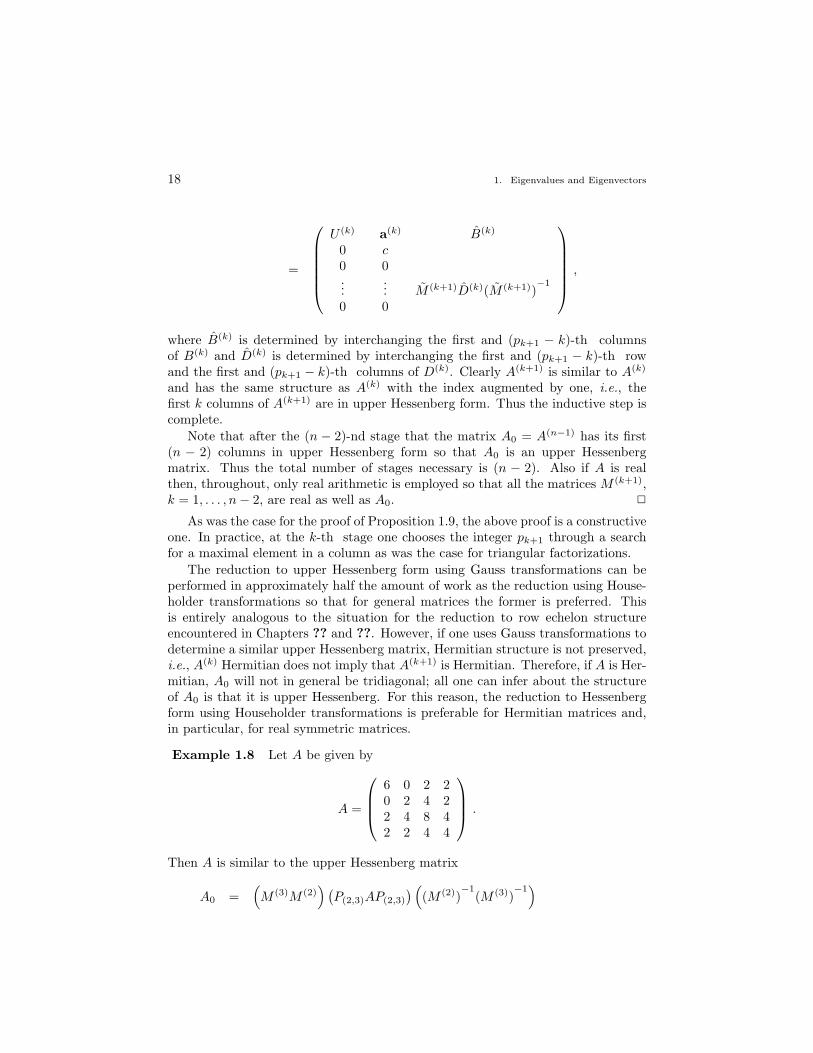
The reduction to upper Hessenberg form using Gauss transformations can beperformed in approximately half the amount of work as the reduction using House-holder transformations so that for general matrices the former is preferred. Thisis entirely analogous to the situation for the reduction to row echelon structureencountered in Chapters ?? and ??. However, if one uses Gauss transformations todetermine a similar upper Hessenberg matrix, Hermitian structure is not preserved,i.e., A(k) Hermitian does not imply that A(k+1) is Hermitian. Therefore, if A is Her-mitian, A0 will not in general be tridiagonal; all one can infer about the structureof A0 is that it is upper Hessenberg. For this reason, the reduction to Hessenbergform using Householder transformations is preferable for Hermitian matrices and,in particular, for real symmetric matrices.
Example 1.8 Let A be given by
A =
6 0 2 20 2 4 22 4 8 42 2 4 4
.
Then A is similar to the upper Hessenberg matrix
A0 =(M (3)M (2)
) (P(2,3)AP(2,3)
) ((M (2))
−1(M (3))
−1)
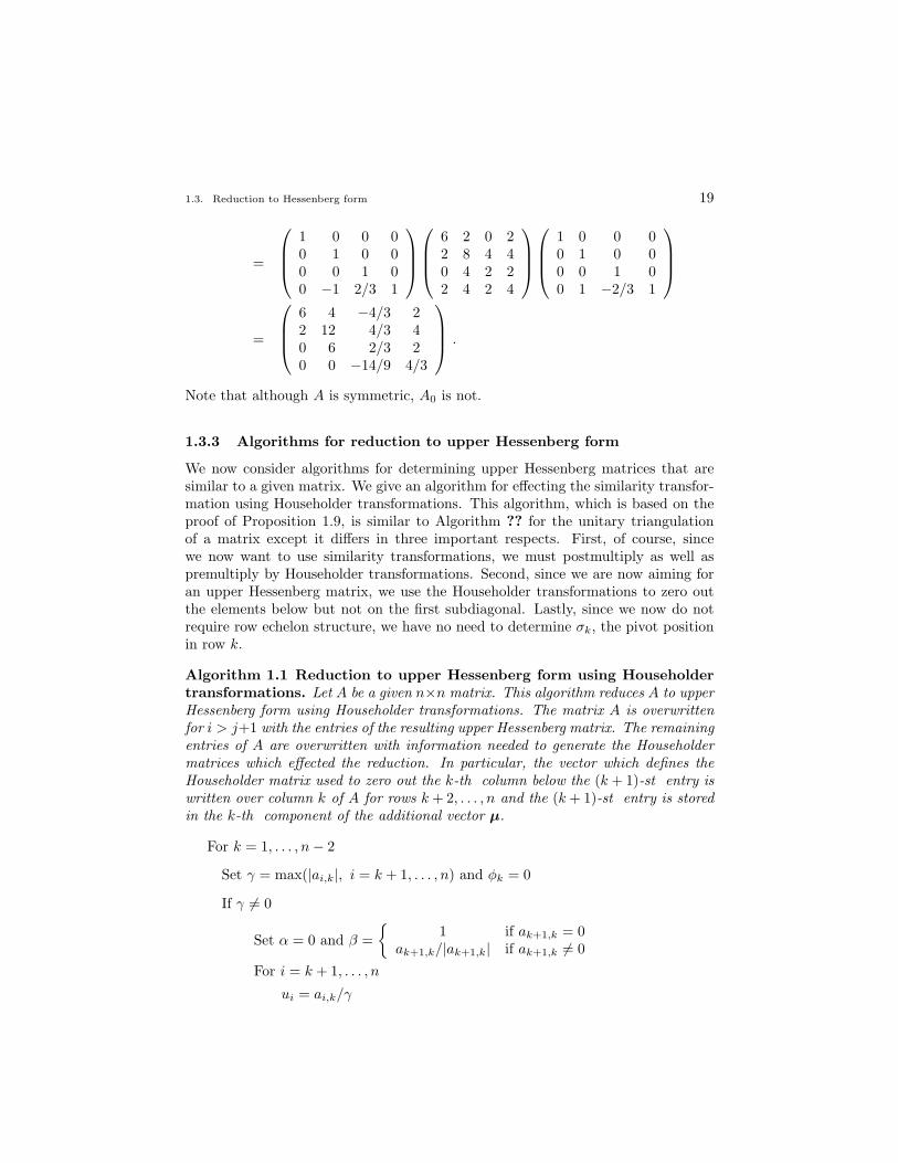
1.3. Reduction to Hessenberg form 19
=
1 0 0 00 1 0 00 0 1 00 −1 2/3 1
6 2 0 22 8 4 40 4 2 22 4 2 4
1 0 0 00 1 0 00 0 1 00 1 −2/3 1
=
6 4 −4/3 22 12 4/3 40 6 2/3 20 0 −14/9 4/3
.
Note that although A is symmetric, A0 is not.
1.3.3 Algorithms for reduction to upper Hessenberg form
We now consider algorithms for determining upper Hessenberg matrices that aresimilar to a given matrix. We give an algorithm for effecting the similarity transfor-mation using Householder transformations. This algorithm, which is based on theproof of Proposition 1.9, is similar to Algorithm ?? for the unitary triangulationof a matrix except it differs in three important respects. First, of course, sincewe now want to use similarity transformations, we must postmultiply as well aspremultiply by Householder transformations. Second, since we are now aiming foran upper Hessenberg matrix, we use the Householder transformations to zero outthe elements below but not on the first subdiagonal. Lastly, since we now do notrequire row echelon structure, we have no need to determine σk, the pivot positionin row k.
Algorithm 1.1 Reduction to upper Hessenberg form using Householdertransformations. Let A be a given n×n matrix. This algorithm reduces A to upperHessenberg form using Householder transformations. The matrix A is overwrittenfor i > j+1 with the entries of the resulting upper Hessenberg matrix. The remainingentries of A are overwritten with information needed to generate the Householdermatrices which effected the reduction. In particular, the vector which defines theHouseholder matrix used to zero out the k-th column below the (k + 1)-st entry iswritten over column k of A for rows k + 2, . . . , n and the (k + 1)-st entry is storedin the k-th component of the additional vector µ.
For k = 1, . . . , n− 2
Set γ = max(|ai,k|, i = k + 1, . . . , n) and φk = 0
If γ 6= 0
Set α = 0 and β ={
1 if ak+1,k = 0ak+1,k/|ak+1,k| if ak+1,k 6= 0
For i = k + 1, . . . , n
ui = ai,k/γ
20 1. Eigenvalues and Eigenvectors
α← α + |ui|2
Set α←√
α
φk = 1/(α(α + |uk+1|)uk+1 ← uk+1 + βα
For s = k + 1, . . . , n
t =n∑
i=k+1
uiai,s
t← φkt
For j = k + 1, . . . , n
aj,s ← aj,s − tuj .
For s = 1, . . . , n
t =n∑
j=k+1
as,juj
t← φkt
For j = k + 1, . . . , n
as,j ← as,j − tuj .
ak+1,k = −α
µk = uk+1
For s = k + 2, . . . , n
as,k = us
k ← k + 1 2
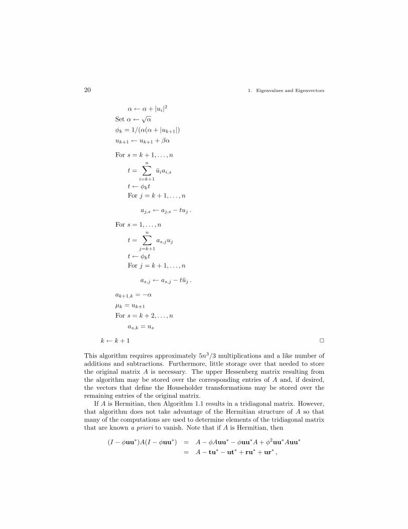
This algorithm requires approximately 5n3/3 multiplications and a like number ofadditions and subtractions. Furthermore, little storage over that needed to storethe original matrix A is necessary. The upper Hessenberg matrix resulting fromthe algorithm may be stored over the corresponding entries of A and, if desired,the vectors that define the Householder transformations may be stored over theremaining entries of the original matrix.
If A is Hermitian, then Algorithm 1.1 results in a tridiagonal matrix. However,that algorithm does not take advantage of the Hermitian structure of A so thatmany of the computations are used to determine elements of the tridiagonal matrixthat are known a priori to vanish. Note that if A is Hermitian, then
(I − φuu∗)A(I − φuu∗) = A− φAuu∗ − φuu∗A + φ2uu∗Auu∗
= A− tu∗ − ut∗ + ru∗ + ur∗ ,
1.3. Reduction to Hessenberg form 21
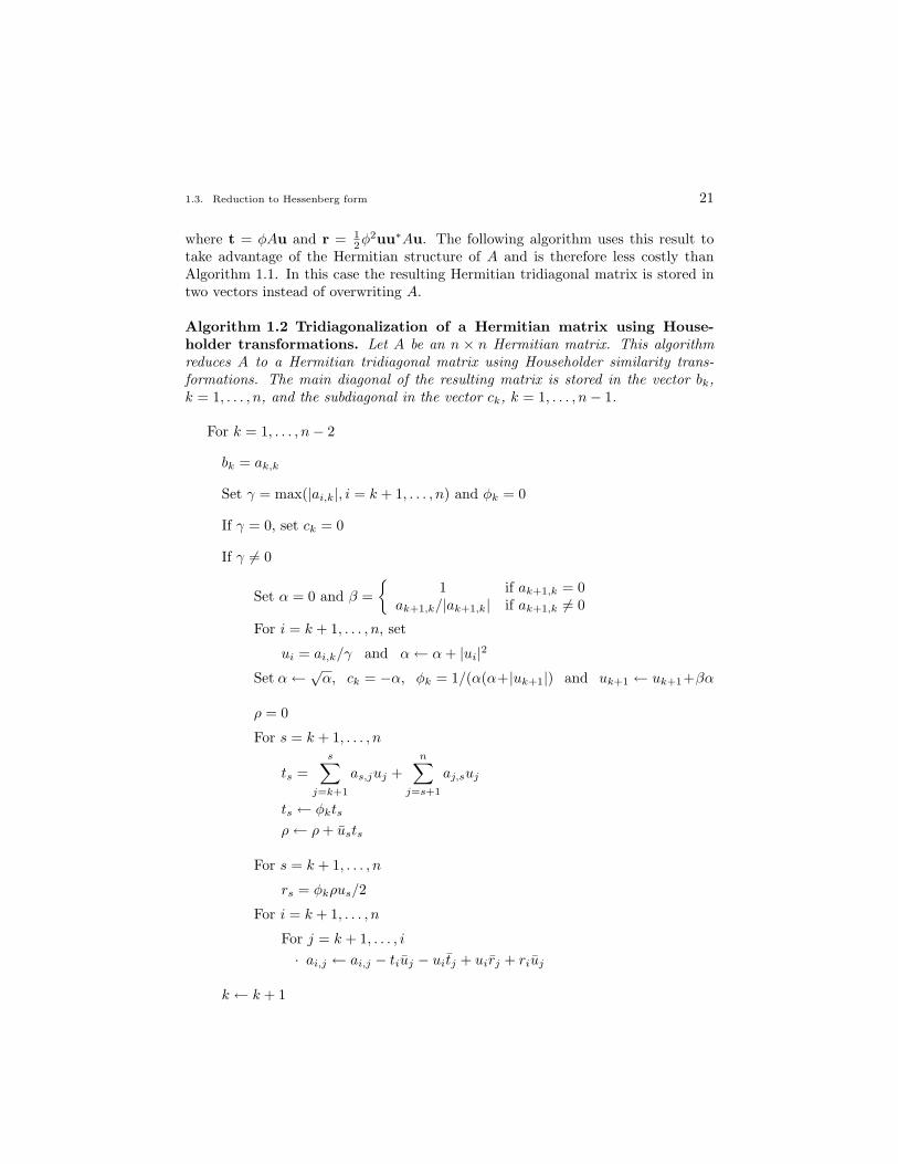
where t = φAu and r = 12φ2uu∗Au. The following algorithm uses this result to
take advantage of the Hermitian structure of A and is therefore less costly thanAlgorithm 1.1. In this case the resulting Hermitian tridiagonal matrix is stored intwo vectors instead of overwriting A.
Algorithm 1.2 Tridiagonalization of a Hermitian matrix using House-holder transformations. Let A be an n × n Hermitian matrix. This algorithmreduces A to a Hermitian tridiagonal matrix using Householder similarity trans-formations. The main diagonal of the resulting matrix is stored in the vector bk,k = 1, . . . , n, and the subdiagonal in the vector ck, k = 1, . . . , n− 1.
For k = 1, . . . , n− 2
bk = ak,k
Set γ = max(|ai,k|, i = k + 1, . . . , n) and φk = 0
If γ = 0, set ck = 0
If γ 6= 0
Set α = 0 and β ={
1 if ak+1,k = 0ak+1,k/|ak+1,k| if ak+1,k 6= 0
For i = k + 1, . . . , n, set
ui = ai,k/γ and α← α + |ui|2
Set α←√
α, ck = −α, φk = 1/(α(α+|uk+1|) and uk+1 ← uk+1+βα
ρ = 0
For s = k + 1, . . . , n
ts =s∑
j=k+1
as,juj +n∑
j=s+1
aj,suj
ts ← φkts
ρ← ρ + usts
For s = k + 1, . . . , n
rs = φkρus/2
For i = k + 1, . . . , n
For j = k + 1, . . . , i
· ai,j ← ai,j − tiuj − uitj + uirj + riuj
k ← k + 1
22 1. Eigenvalues and Eigenvectors
Set cn−1 = an,n−1 , bn−1 = an−1,n−1 , and bn = an,n. 2
This algorithm requires only about 2n3/3 multiplications and a like number ofadditions and subtractions. Again, an efficient storage scheme is possible, i.e.,the numbers that define the tridiagonal result of the algorithm and the vectors thatdefine the Householder transformations may be stored in the same locations as thoseoriginally used to store either the upper of lower triangular parts of the Hermitianmatrix A.
We close this section by remarking that an algorithm for similarity reduction toupper Hessenberg form using Gauss transformations can be easily developed. Thisalgorithm is similar to Algorithm 1.1 except now we use the pivoting strategiesand Gauss transformations matrices of Algorithm ??. An analysis of the operationcount demonstrates that the similarity reduction to upper Hessenberg form usingGauss transformations requires approximately one-half the work of the reductionusing Householder transformations.
1.4 Methods for computing a few eigenvalues and eigenvec-tors
In this section we consider techniques for finding one or a few eigenvalues andcorresponding eigenvectors of an n×n matrix. Most of the methods we discuss arebased on the power method, a simple iterative scheme involving increasing powersof the matrix. Included in this class of methods are the inverse power method,the Rayleigh quotient iteration, and subspace iteration. In addition we consider amethod based on Sturm sequences which is applicable to finding some eigenvaluesof Hermitian tridiagonal matrices. If most or all of the eigenvalues and eigenvectorsare desired, then the QR method considered in Section 1.5 is preferred.
1.4.1 The power method
The power method is a means for determining an eigenvector corresponding to theeigenvalue of largest modulus. It also forms the basis for the definition of othermethods for eigenvalue/eigenvector determination and is a necessary ingredient inthe analysis of many such methods. However, the iterates determined by the powermethod may converge extremely slowly, and sometimes may fail to converge.
Let A be an n×n matrix. We first consider in some detail the power method forthe case when A is nondefective, i.e., A has a complete set of linearly independenteigenvectors. For example, if A is Hermitian then it satisfies this condition. Thebasic algorithm is to choose an initial vector q(0) 6= 0 ∈ Cn and then generate theiterates by
q(k) =1αk
Aq(k−1) for k = 1, 2, . . . ,(1.20)
where αk, k = 1, 2, . . ., are scale factors. One choice for the scale factor αk is the
1.4. Methods for computing a few eigenvalues and eigenvectors 23
component of the vector Aq(k−1) which has the maximal absolute value, i.e.,
αk = (Aq(k−1))p for k = 1, 2, . . . ,(1.21)
where p is the smallest integer such that
|(Aq(k−1))p| = maxj=1,...,n
|(Aq(k−1))j | = ‖Aq(k−1)‖∞ .
Another choice for the scale factor αk is the product of the Euclidean length ofthe vector Aq(k−1) and the phase (the sign if A and q(k−1) are real) of a nonzerocomponent of Aq(k−1) . Specifically, we have
αk =(Aq(k−1))`
|(Aq(k−1))`|√
(Aq(k−1))∗(Aq(k−1))
=(Aq(k−1))`
|(Aq(k−1))`|‖Aq(k−1)‖2 for k = 1, 2, . . . ,
(1.22)
where we choose ` to be the smallest component index such that
|(Aq(k−1))`|/‖Aq(k−1)‖2 ≥ 1/n .
Such an `, 1 ≤ ` ≤ n, exists by virtue of the fact that Aq(k−1)/‖Aq(k−1)‖2 is a unitvector. We shall see below that the scale factors αk are used to avoid underflows oroverflows during the calculations of the power method iterates q(k) for k ≥ 1. Thescale factor αk often is chosen according to αk = ‖(Aq(k−1)‖∞ or αk = ‖Aq(k−1)‖2,and not by (1.21) or (1.22), respectively. Below, we will examine why the choices(1.21) or (1.22) are preferable.
Let {x(1),x(2), . . . ,x(n)} denote a linearly independent set of n eigenvectors ofA corresponding to the eigenvalues λj , j = 1, . . . , n; such a set exists by virtue ofthe assumption that A is nondefective. This set forms a basis for Cn so that wecan express q(0) as a linear combination of the eigenvectors x(i), i.e.,
q(0) = c1x(1) + c2x(2) + · · ·+ cnx(n)(1.23)
for some complex-valued constants c1, c2, . . . , cn.If A and q(0) are real, then with either choice (1.21) or (1.22) for the scale
factors, the iterates q(k), k = 1, 2, . . . , are real as well. Thus, immediately, one seesa potential difficulty with the power method: if the initial vector is chosen to bereal, it is impossible for the iterates of the power method to converge to a complexeigenvector of a real matrix A. We will discuss this in more detail below. For nowwe assume that the eigenvalues of A satisfy
λ1 = λ2 = · · · = λm(1.24)
and|λ1| > |λm+1| ≥ |λm+2| ≥ · · · ≥ |λn| .(1.25)
24 1. Eigenvalues and Eigenvectors
These imply that the dominant eigenvalue λ1 is unique, nonvanishing, and hasalgebraic multiplicity m. Since A is nondefective, λ1 also has geometric multiplicitym and {x(1),x(2), . . . ,x(m)} then denotes a set of linearly independent eigenvectorscorresponding to λ1. (Note that if A is real, then, as a result of (1.24) and (1.25),λ1 is necessarily real and the vectors x(j), j = 1, . . . ,m, may be chosen to be realas well.) Under these assumptions we can show that if the scale factors αk arechosen by either (1.21) or (1.22), then the sequence q(0),q(1), . . . ,q(k), . . . of powermethod iterates converges to an eigenvector corresponding to λ1. To do this wewill demonstrate that ‖q(k) − q‖2 = O
(|λm+1/λ1|k
)for k = 1, 2, . . . , where the
notation γ(k) = O(β(k)) implies that the ratio γ(k)/β(k) remains finite as k →∞.
Proposition 1.13 Let A be a nondefective n × n matrix; denote its eigenvaluesand corresponding eigenvectors by λj and x(j), j = 1, . . . , n, respectively. Letthe eigenvalues of A satisfy (1.24) and (1.25). Let q(0) be a given initial vec-tor such that
∑mj=1 |cj | 6= 0, where the constants cj, j = 1, . . . ,m, are defined
through (1.23). Let the scale factors αk, k = 1, 2, . . ., be defined by either (1.21) or(1.22). Let the sequence of vectors {q(k)}, k = 1, 2, . . ., be defined by (1.20), i.e.,q(k) = (1/αk)Aq(k−1) for k = 1, 2, . . . . Then there exists an eigenvector q of Acorresponding to λ1 such that
‖q(k) − q‖2 = O
(∣∣∣∣λm+1
λ1
∣∣∣∣k)
for k = 1, 2, . . . ,(1.26)
i.e., as k →∞, q(k) converges to an eigenvector q of A corresponding to the uniquedominant eigenvalue λ1. If A is real and the initial vector q(0) is chosen to be real,then all subsequent iterates q(k), k = 1, 2, . . ., are real as well and converge to a realeigenvector of A corresponding to the real dominant eigenvalue λ1.
Proof. Since
q(k) =1αk
Aq(k−1) =1
αkαk−1A2q(k−2) = · · · = (
k∏j=1
1αj
)Akq(0)
and λ1 = λ2 = · · · = λm, we have that
q(k) =
k∏j=1
1αj
Ak(c1x(1) + c2x(2) + · · ·+ cnx(n)
)
=
k∏j=1
1αj
(c1λk1x
(1) + c2λk2x
(2) + · · ·+ cnλknx(n))
= λk1
k∏j=1
1αj
m∑j=1
cjx(j) +n∑
j=m+1
(λj
λ1
)k
cjx(j)
,(1.27)
1.4. Methods for computing a few eigenvalues and eigenvectors 25
where we have used the fact that if λ is an eigenvalue of A with corrrespondingeigenvector x, then λk is an eigenvalue of Ak with the same corresponding eigen-vector. Then, since |λm+1| ≥ |λj | for j = m + 2, . . . , n,
q(k) = λk1
k∏j=1
1αj
m∑j=1
cjx(j) + O
(∣∣∣∣λm+1
λ1
∣∣∣∣k) for k = 1, 2, . . . .(1.28)
Now, for the choice (1.21) for the scale factors, it follows from (1.28) and∑mj=1 |cj | 6= 0 that
‖q(k) − q‖2 = O
(∣∣∣∣λm+1
λ1
∣∣∣∣k)
for k = 1, 2, . . . ,(1.29)
where
q =x‖x‖∞
with x =m∑
j=1
cjx(j) .(1.30)
Since x(j), j = 1, . . . ,m, are all eigenvectors corresponding to the same eigen-value λ1, then q defined by (1.30) is also an eigenvector of A corresponding to λ1.Then (1.26) holds with q given by (1.30) and, since |λ1| > |λm+1|, it follows from(1.29) that the power method iterates q(k) converge as k →∞ to an eigenvector qof A corresponding to the dominant eigenvalue λ1.
The same result holds for the choice (1.22) for the scale factors, except that now
q =|x`|
x`‖x‖2x with x =
m∑j=1
cjx(j)(1.31)
where ` is the smallest index such that x`/‖x‖2 ≥ 1/n .If A is real, it follows from the hypotheses that λ1 is real. If q(0) is also real,
then clearly all subsequent iterates are real. The eigenvectors corresponding to λ1
may be chosen to be real in which case the constants cj , j = 1, . . . ,m, in (1.23) arenecessarily real. Then, as a result of (1.28), the power method iterates converge toa real eigenvector of A. 2
We now consider the choices (1.21) and (1.22) for the scale factors αk, k ≥ 1,in more detail. First, we note that if αk = 1 for all k, then instead of (1.29) and(1.30) or (1.31), we would have that
q(k) → λk1
m∑j=1
cjx(j) as k →∞ .(1.32)
If |λ1| 6= 1, then λk1 tends to infinity or zero as k → ∞. On a computer, this
may cause overflows or underflows if q(k) satisfies (1.32). On the other hand, if the
26 1. Eigenvalues and Eigenvectors
choice (1.21) is made for the scale factors, then it follows that ‖q(k))‖∞ = 1 for allk so that one avoids overflow or underflow problems due to the growth or decayof λk
1 . (In fact, in the latter case, the maximal element is actually equal to unity.)Similarly, these overflow or underflow problems are avoided for the choice (1.22) forthe scale factors since in this case ‖q(k)‖2 = 1 for all k so that 1/n ≤ ‖q(k)‖∞ ≤ 1for all k.
These underflow and overflow problems are also avoided for the choices αk =‖Aq(k−1))‖∞ or αk = ‖Aq(k−1)‖2. However, if we choose αk = ‖Aq(k−1))‖∞instead of (1.21), we then obtain
q(k) →
(λ1
k
|λ1|k
)x‖x‖∞
as k →∞ ,(1.33)
instead of (1.29) and (1.30), where again we have set x =m∑
j=1
cjx(j). Similarly, if
we choose αk = ‖Aq(k−1)‖2 instead of (1.22), we then obtain
q(k) →
(λ1
k
|λ1|k
)x‖x‖2
(1.34)
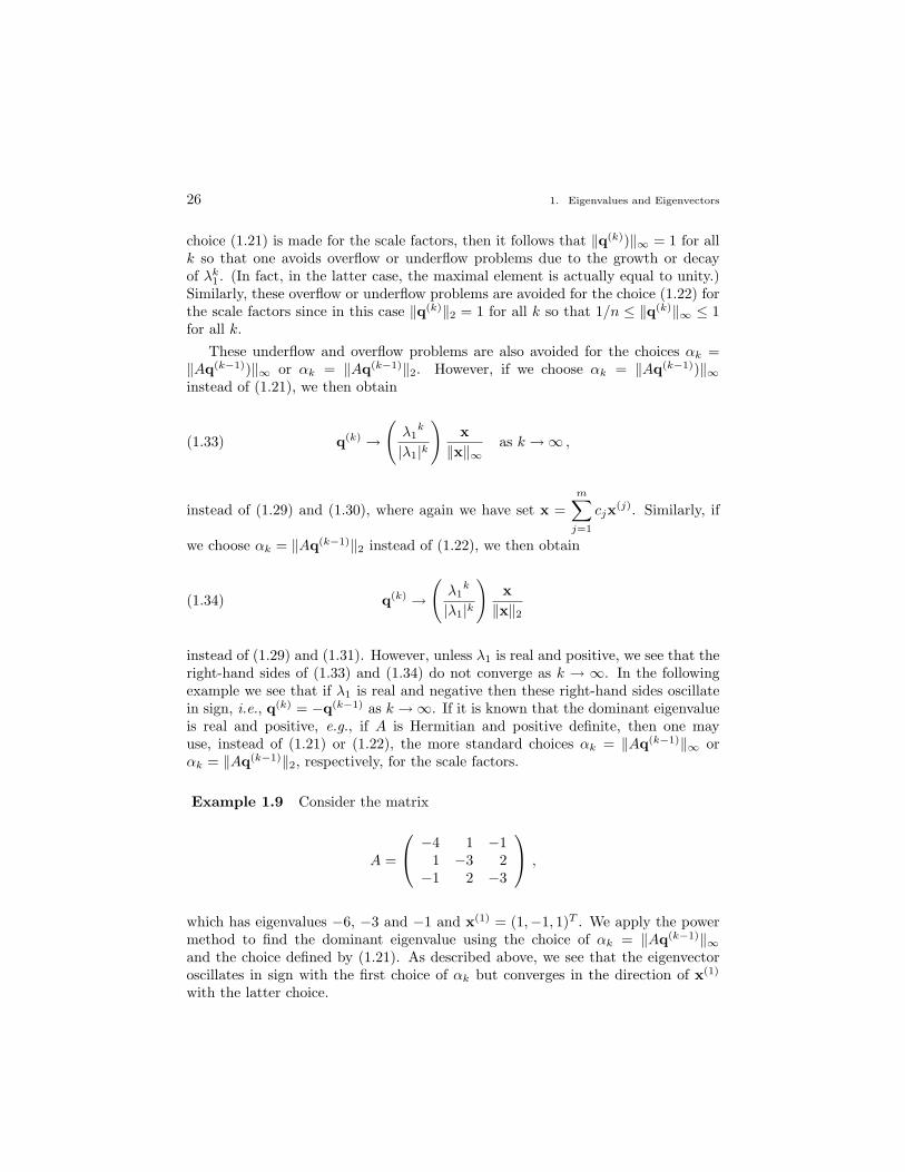
instead of (1.29) and (1.31). However, unless λ1 is real and positive, we see that theright-hand sides of (1.33) and (1.34) do not converge as k → ∞. In the followingexample we see that if λ1 is real and negative then these right-hand sides oscillatein sign, i.e., q(k) = −q(k−1) as k →∞. If it is known that the dominant eigenvalueis real and positive, e.g., if A is Hermitian and positive definite, then one mayuse, instead of (1.21) or (1.22), the more standard choices αk = ‖Aq(k−1)‖∞ orαk = ‖Aq(k−1)‖2, respectively, for the scale factors.
Example 1.9 Consider the matrix
A =
−4 1 −11 −3 2−1 2 −3
,
which has eigenvalues −6, −3 and −1 and x(1) = (1,−1, 1)T . We apply the powermethod to find the dominant eigenvalue using the choice of αk = ‖Aq(k−1)‖∞and the choice defined by (1.21). As described above, we see that the eigenvectoroscillates in sign with the first choice of αk but converges in the direction of x(1)
with the latter choice.
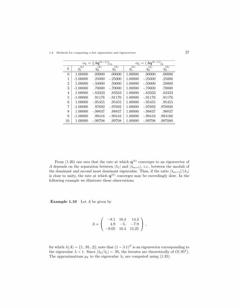
1.4. Methods for computing a few eigenvalues and eigenvectors 27
αk = ‖Aq(k−1)‖∞ αk = (Aq(k−1))p
k q(k)1 q
(k)2 q
(k)3 q
(k)1 q
(k)2 q
(k)3
0 1.00000 .00000 .00000 1.00000 .00000 .000001 -1.00000 .25000 -.25000 1.00000 -.25000 .250002 1.00000 -.50000 .50000 1.00000 -.50000 .500003 -1.00000 .70000 -.70000 1.00000 -.70000 .700004 1.00000 -.83333 .83333 1.00000 -.83333 .833335 -1.00000 .91176 -.91176 1.00000 -.91176 .911766 1.00000 -.95455 .95455 1.00000 -.95455 .954557 -1.00000 .97692 -.97692 1.00000 -.97692 .9769208 1.00000 -.98837 .98837 1.00000 -.98837 .988379 -1.00000 .99416 -.99416 1.00000 -.99416 .994160
10 1.00000 -.99708 .99708 1.00000 -.99708 .997080
From (1.26) one sees that the rate at which q(k) converges to an eigenvector ofA depends on the separation between |λ1| and |λm+1|, i.e., between the moduli ofthe dominant and second most dominant eigenvalue. Thus, if the ratio |λm+1|/|λ1|is close to unity, the rate at which q(k) converges may be exceedingly slow. In thefollowing example we illustrate these observations.
Example 1.10 Let A be given by
A =
−8.1 10.4 14.34.9 −5. −7.9
−9.05 10.4 15.25
,
for which λ(A) = {1, .95, .2}; note that (1−.5 1)T is an eigenvector corresponding tothe eigenvalue λ = 1. Since |λ2/λ1| = .95, the iterates are theoretically of O(.95k).The approximations µk to the eigenvalue λ1 are computed using (1.35).
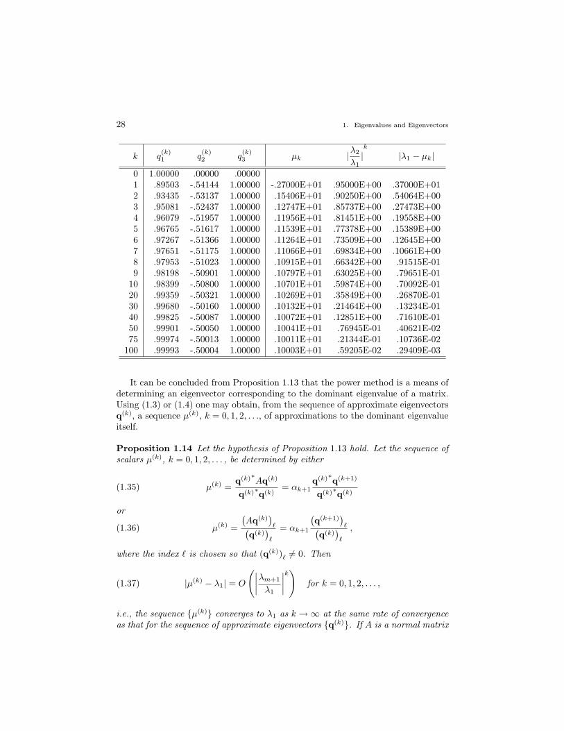
28 1. Eigenvalues and Eigenvectors
k q(k)1 q
(k)2 q
(k)3 µk |λ2
λ1|k
|λ1 − µk|
0 1.00000 .00000 .000001 .89503 -.54144 1.00000 -.27000E+01 .95000E+00 .37000E+012 .93435 -.53137 1.00000 .15406E+01 .90250E+00 .54064E+003 .95081 -.52437 1.00000 .12747E+01 .85737E+00 .27473E+004 .96079 -.51957 1.00000 .11956E+01 .81451E+00 .19558E+005 .96765 -.51617 1.00000 .11539E+01 .77378E+00 .15389E+006 .97267 -.51366 1.00000 .11264E+01 .73509E+00 .12645E+007 .97651 -.51175 1.00000 .11066E+01 .69834E+00 .10661E+008 .97953 -.51023 1.00000 .10915E+01 .66342E+00 .91515E-019 .98198 -.50901 1.00000 .10797E+01 .63025E+00 .79651E-01
10 .98399 -.50800 1.00000 .10701E+01 .59874E+00 .70092E-0120 .99359 -.50321 1.00000 .10269E+01 .35849E+00 .26870E-0130 .99680 -.50160 1.00000 .10132E+01 .21464E+00 .13234E-0140 .99825 -.50087 1.00000 .10072E+01 .12851E+00 .71610E-0150 .99901 -.50050 1.00000 .10041E+01 .76945E-01 .40621E-0275 .99974 -.50013 1.00000 .10011E+01 .21344E-01 .10736E-02
100 .99993 -.50004 1.00000 .10003E+01 .59205E-02 .29409E-03
It can be concluded from Proposition 1.13 that the power method is a means ofdetermining an eigenvector corresponding to the dominant eigenvalue of a matrix.Using (1.3) or (1.4) one may obtain, from the sequence of approximate eigenvectorsq(k), a sequence µ(k), k = 0, 1, 2, . . ., of approximations to the dominant eigenvalueitself.
Proposition 1.14 Let the hypothesis of Proposition 1.13 hold. Let the sequence ofscalars µ(k), k = 0, 1, 2, . . . , be determined by either
µ(k) =q(k)∗Aq(k)
q(k)∗q(k)= αk+1
q(k)∗q(k+1)
q(k)∗q(k)(1.35)
or
µ(k) =
(Aq(k)
)`(
q(k))`
= αk+1
(q(k+1)
)`(
q(k))`
,(1.36)
where the index ` is chosen so that (q(k))` 6= 0. Then
|µ(k) − λ1| = O
(∣∣∣∣λm+1
λ1
∣∣∣∣k)
for k = 0, 1, 2, . . . ,(1.37)
i.e., the sequence {µ(k)} converges to λ1 as k →∞ at the same rate of convergenceas that for the sequence of approximate eigenvectors {q(k)}. If A is a normal matrix
1.4. Methods for computing a few eigenvalues and eigenvectors 29
so that A possesses an orthonormal set of eigenvectors, and if the approximateeigenvalues µ(k) are chosen according to (1.35), then
|µ(k) − λ1| = O
(∣∣∣∣λm+1
λ1
∣∣∣∣2k)
for k = 0, 1, 2, . . . .(1.38)
Proof. First, let µ(k) be determined by (1.35). It is easily seen that
µ(k) =q(k)∗Aq(k)
q(k)∗q(k)
=
(∑nj=1 cjλj
kx(j))∗ (∑n
j=1 cjλjk+1x(j)
)(∑n
j=1 cjλjkx(j)
)∗ (∑nj=1 cjλj
kx(j))(1.39)
= λ1 + O
(∣∣∣∣λm+1
λ1
∣∣∣∣k)
so that (1.37) is valid. If the eigenvectors {x(j)}nj=1 are orthonormal, then from(1.39)
µ(k) =
∑nj=1 λj |cjλj
k|2∑nj=1 |cjλj
k|2= λ1
∑mj=1 |cj |2 + O(|λm+1/λ1|2k)∑mj=1 |cj |2 + O(|λm+1/λ1|2k)
so that (1.38) holds.Now, let µ(k) be determined (1.36). Then it is easily seen that
µ(k) =(Aq(k))`
(q(k))`=
(∑nj=1 cjλj
k+1x(j))
`(∑nj=1 cjλj
kx(j))
`
= λ1
(∑mj=1 cjx(j)
)`+ O(|λm+1/λ1|k)(∑m
j=1 cjx(j))
`+ O(|λm+1/λ1|k)
so that (1.38) is valid. 2
Thus, if A is normal, e.g., Hermitian or skew-Hermitian, the use of (1.35) ispreferable to that of (1.36). Also, note that with either (1.35) or (1.36) we havethat µ(k) − αk+1 → 0 as k → ∞ so that, using (1.38), we may conclude that thescale factors αk+1 converge to the eigenvalue λ1.
We have analyzed the power method for the case where a given matrix A isnondefective and has a unique dominant eigenvalue. We now discuss the behaviorof the power method iterates when the assumptions of Proposition 1.13 do nothold. First, let us see that the convergence of the power method is essentiallyunaffected if eigenvalues other than the dominant eigenvalue are defective. For
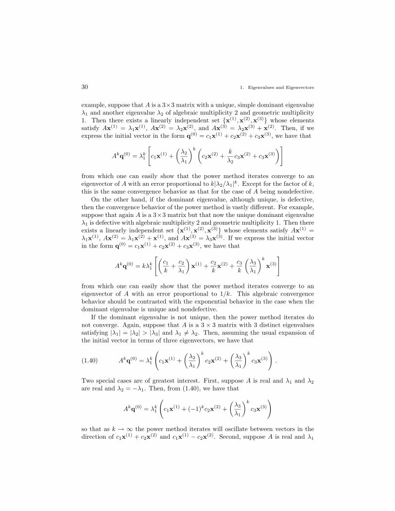
30 1. Eigenvalues and Eigenvectors
example, suppose that A is a 3×3 matrix with a unique, simple dominant eigenvalueλ1 and another eigenvalue λ2 of algebraic multiplicity 2 and geometric multiplicity1. Then there exists a linearly independent set {x(1),x(2),x(3)} whose elementssatisfy Ax(1) = λ1x(1), Ax(2) = λ2x(2), and Ax(3) = λ2x(3) + x(2). Then, if weexpress the initial vector in the form q(0) = c1x(1) + c2x(2) + c3x(3), we have that
Akq(0) = λk1
[c1x(1) +
(λ2
λ1
)k (c2x(2) +
k
λ2c3x(2) + c3x(3)
)]
from which one can easily show that the power method iterates converge to aneigenvector of A with an error proportional to k|λ2/λ1|k. Except for the factor of k,this is the same convergence behavior as that for the case of A being nondefective.
On the other hand, if the dominant eigenvalue, although unique, is defective,then the convergence behavior of the power method is vastly different. For example,suppose that again A is a 3×3 matrix but that now the unique dominant eigenvalueλ1 is defective with algebraic multiplicity 2 and geometric multiplicity 1. Then thereexists a linearly independent set {x(1),x(2),x(3)} whose elements satisfy Ax(1) =λ1x(1), Ax(2) = λ1x(2) + x(1), and Ax(3) = λ3x(3). If we express the initial vectorin the form q(0) = c1x(1) + c2x(2) + c3x(3), we have that
Akq(0) = kλk1
[(c1
k+
c2
λ1
)x(1) +
c2
kx(2) +
c3
k
(λ3
λ1
)k
x(3)
]
from which one can easily show that the power method iterates converge to aneigenvector of A with an error proportional to 1/k. This algebraic convergencebehavior should be contrasted with the exponential behavior in the case when thedominant eigenvalue is unique and nondefective.
If the dominant eigenvalue is not unique, then the power method iterates donot converge. Again, suppose that A is a 3 × 3 matrix with 3 distinct eigenvaluessatisfying |λ1| = |λ2| > |λ3| and λ1 6= λ2. Then, assuming the usual expansion ofthe initial vector in terms of three eigenvectors, we have that
Akq(0) = λk1
(c1x(1) +
(λ2
λ1
)k
c2x(2) +(
λ3
λ1
)k
c3x(3)
).(1.40)
Two special cases are of greatest interest. First, suppose A is real and λ1 and λ2
are real and λ2 = −λ1. Then, from (1.40), we have that
Akq(0) = λk1
(c1x(1) + (−1)kc2x(2) +
(λ3
λ1
)k
c3x(3)
)
so that as k → ∞ the power method iterates will oscillate between vectors in thedirection of c1x(1) + c2x(2) and c1x(1) − c2x(2). Second, suppose A is real and λ1
1.4. Methods for computing a few eigenvalues and eigenvectors 31
and λ2 are complex so that λ1 = λ2 = |λ1|eiθ. Also, assume that q(0) is real so thatq(0) = c1x(1) + c1x(1) + c3x(3) and, from (1.40),
Akq(0) = λk1
(c1x(1) + c1e
−2ikθx(1) +(
λ3
λ1
)k
c3x(3)
).
Again, it is clear that the iterates will not converge, even in direction.
It should be noted that even in these cases in which the power method doesnot converge, it is possible to combine information gleaned from a few successiveiterates to determine a convergent subsequence.
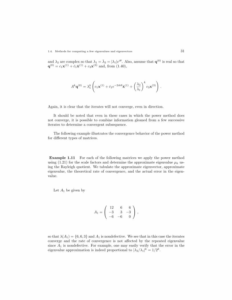
The following example illustrates the convergence behavior of the power methodfor different types of matrices.
Example 1.11 For each of the following matrices we apply the power methodusing (1.21) for the scale factors and determine the approximate eigenvalue µk us-ing the Rayleigh quotient. We tabulate the approximate eigenvector, approximateeigenvalue, the theoretical rate of convergence, and the actual error in the eigen-value.
Let A1 be given by
A1 =
12 6 6−3 3 −3−6 −6 0
,
so that λ(A1) = {6, 6, 3} and A1 is nondefective. We see that in this case the iteratesconverge and the rate of convergence is not affected by the repeated eigenvaluesince A1 is nondefective. For example, one may easily verify that the error in theeigenvalue approximation is indeed proportional to |λ3/λ1|k = 1/2k.
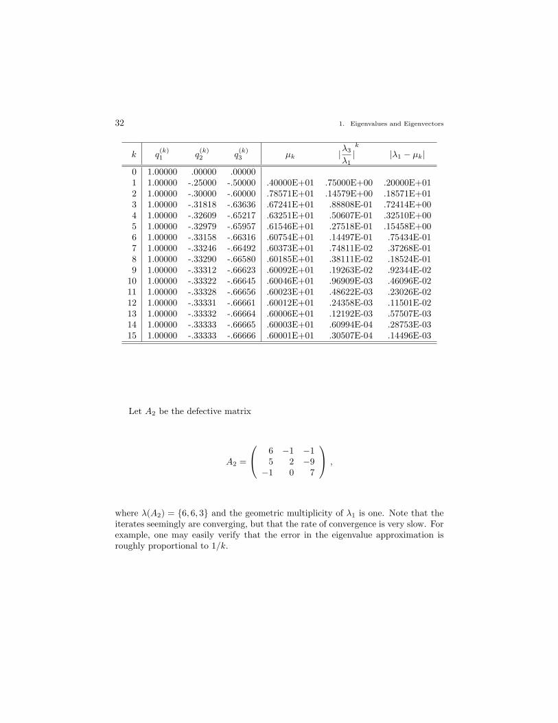
32 1. Eigenvalues and Eigenvectors
k q(k)1 q
(k)2 q
(k)3 µk |λ3
λ1|k
|λ1 − µk|
0 1.00000 .00000 .000001 1.00000 -.25000 -.50000 .40000E+01 .75000E+00 .20000E+012 1.00000 -.30000 -.60000 .78571E+01 .14579E+00 .18571E+013 1.00000 -.31818 -.63636 .67241E+01 .88808E-01 .72414E+004 1.00000 -.32609 -.65217 .63251E+01 .50607E-01 .32510E+005 1.00000 -.32979 -.65957 .61546E+01 .27518E-01 .15458E+006 1.00000 -.33158 -.66316 .60754E+01 .14497E-01 .75434E-017 1.00000 -.33246 -.66492 .60373E+01 .74811E-02 .37268E-018 1.00000 -.33290 -.66580 .60185E+01 .38111E-02 .18524E-019 1.00000 -.33312 -.66623 .60092E+01 .19263E-02 .92344E-02
10 1.00000 -.33322 -.66645 .60046E+01 .96909E-03 .46096E-0211 1.00000 -.33328 -.66656 .60023E+01 .48622E-03 .23026E-0212 1.00000 -.33331 -.66661 .60012E+01 .24358E-03 .11501E-0213 1.00000 -.33332 -.66664 .60006E+01 .12192E-03 .57507E-0314 1.00000 -.33333 -.66665 .60003E+01 .60994E-04 .28753E-0315 1.00000 -.33333 -.66666 .60001E+01 .30507E-04 .14496E-03
Let A2 be the defective matrix
A2 =
6 −1 −15 2 −9−1 0 7
,
where λ(A2) = {6, 6, 3} and the geometric multiplicity of λ1 is one. Note that theiterates seemingly are converging, but that the rate of convergence is very slow. Forexample, one may easily verify that the error in the eigenvalue approximation isroughly proportional to 1/k.
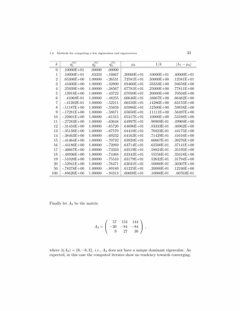
1.4. Methods for computing a few eigenvalues and eigenvectors 33
k q(k)1 q
(k)2 q
(k)3 µk 1/k |λ1 − µk|
0 .10000E+01 .00000 .000001 .10000E+01 .83333 -.16667 .20000E+01 .10000E+01 .40000E+012 .65306E+00 1.00000 -.26531 .72581E+01 .50000E+00 .12581E+013 .41600E+00 1.00000 -.32800 .69466E+01 .33333E+00 .94658E+004 .25939E+00 1.00000 -.38567 .67781E+01 .25000E+00 .77811E+005 .13918E+00 1.00000 -.43722 .67050E+01 .20000E+00 .70504E+006 .41068E-01 1.00000 -.48255 .66646E+01 .16667E+00 .66462E+007 -.41392E-01 1.00000 -.52211 .66316E+01 .14286E+00 .63155E+008 -.11187E+00 1.00000 -.55659 .65986E+01 .12500E+00 .59858E+009 -.17281E+00 1.00000 -.58671 .65650E+01 .11111E+00 .56497E+00
10 -.22601E+00 1.00000 -.61315 .65317E+01 .10000E+00 .53168E+0011 -.27283E+00 1.00000 -.63648 .64997E+01 .90909E-01 .49969E+0012 -.31434E+00 1.00000 -.65720 .64696E+01 .83333E-01 .46962E+0013 -.35138E+00 1.00000 -.67570 .64418E+01 .76923E-01 .44175E+0014 -.38463E+00 1.00000 -.69232 .64162E+01 .71429E-01 .41616E+0015 -.41464E+00 1.00000 -.70732 .63928E+01 .66667E-01 .39276E+0016 -.44186E+00 1.00000 -.72093 .63714E+01 .62500E-01 .37141E+0017 -.46667E+00 1.00000 -.73333 .63519E+01 .58824E-01 .35195E+0018 -.48936E+00 1.00000 -.74468 .63342E+01 .55556E-01 .33418E+0019 -.51020E+00 1.00000 -.75510 .63179E+01 .52632E-01 .31794E+0020 -.52941E+00 1.00000 -.76471 .63031E+01 .50000E-01 .30307E+0050 -.78378E+00 1.00000 -.89189 .61225E+01 .20000E-01 .12246E+00
100 -.88626E+00 1.00000 -.94313 .60608E+01 .10000E-01 .60763E-01
Finally let A3 be the matrix
A3 =
57 153 144−30 −84 −84
9 27 30
,
where λ(A3) = {6,−6, 3}, i.e., A3 does not have a unique dominant eigenvalue. Asexpected, in this case the computed iterates show no tendency towards converging.
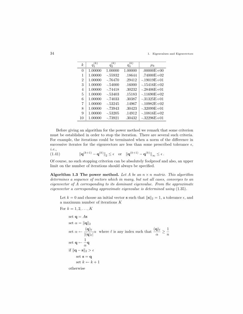
34 1. Eigenvalues and Eigenvectors
k q(k)1 q
(k)2 q
(k)3 µk
0 1.00000 1.00000 1.00000 .00000E+001 1.00000 -.55932 .18644 .74000E+022 1.00000 -.76470 .29412 -.19019E+013 1.00000 -.54000 .16000 -.15416E+024 1.00000 -.74418 .30232 -.28406E+015 1.00000 -.53403 .15183 -.11690E+026 1.00000 -.74033 .30387 -.31325E+017 1.00000 -.53245 .14967 -.10982E+028 1.00000 -.73943 .30423 -.32099E+019 1.00000 -.53205 .14912 -.10816E+02
10 1.00000 -.73921 .30432 -.32296E+01
Before giving an algorithm for the power method we remark that some criterionmust be established in order to stop the iteration. There are several such criteria.For example, the iterations could be terminated when a norm of the difference insuccessive iterates for the eigenvectors are less than some prescribed tolerance ε,i.e.,
‖q(k+1) − q(k)‖2 ≤ ε or ‖q(k+1) − q(k)‖∞ ≤ ε .(1.41)
Of course, no such stopping criterion can be absolutely foolproof and also, an upperlimit on the number of iterations should always be specified.
Algorithm 1.3 The power method. Let A be an n× n matrix. This algorithmdetermines a sequence of vectors which in many, but not all cases, converges to aneigenvector of A corresponding to its dominant eigenvalue. From the approximateeigenvector a corresponding approximate eigenvalue is determined using (1.35).
Let k = 0 and choose an initial vector s such that ‖s‖2 = 1, a tolerance ε, anda maximum number of iterations K
For k = 1, 2, . . . ,K
set q = As
set α = ‖q‖2
set α← (q)`
|(q)`|α where ` is any index such that
(q)`
α≥ 1
n
set q← 1αq
if ‖q− s‖2 > ε
set s = qset k ← k + 1
otherwise
1.4. Methods for computing a few eigenvalues and eigenvectors 35
set λ = αs∗q then stop . 2
If it is known that the dominant eigenvalue is real and positive, i.e., if A isa symmetric positive definite matrix, then the step involving the index ` may beomitted.
1.4.2 Inverse power method
We have seen that the power method provides a means for determining an eigenvec-tor corresponding to the dominant eigenvalue of a matrix. If the power method isapplied to the inverse of a given matrix, one would expect the iterates to convergeto an eigenvector corresponding to the dominant eigenvalue of the inverse matrix,or, equivalently, corresponding to the least dominant eigenvalue of the original ma-trix. This observation leads us to the inverse power method. Another novel featurethat may be incorporated into this algorithm is an eigenvalue shift that, in princi-ple, can be used to force the inverse power iterates to converge to an eigenvectorcorresponding to any eigenvalue one chooses. (Shift strategies may also be used inconjunction with the ordinary power method, but there their utility is not so greatas it is for the inverse power method.)
Let A be a nondefective n×n matrix and let µ be a given scalar; one can view µas being a guess for an eigenvalue of A. Let λj , j = 1, . . . , n, denote the eigenvaluesof A. For simplicity, we assume that there is a unique eigenvalue closest to µ, i.e.,there is an integer r such that 1 ≤ r ≤ n and such that
|λr − µ| ≤ |λj − µ| for j = 1, . . . , n, j 6= r, with
|λr − µ| = |λj − µ| if and only if λj = λr .(1.42)
The behavior of the inverse power method in more general situations, e.g., A beingdefective or the eigenvalue λr being non-unique, can be determined in a similarmanner to that for the power method.
Consider the matrix (A− µI)−1 which has eigenvalues 1/(λj − µ), j = 1, . . . , n.We now apply the power method to this matrix. Thus, given an initial vector q(0),we determine q(k) for k = 1, 2, . . ., from
q(k) =1βk
(A− µI)−1q(k−1) for k = 1, 2, . . .
or equivalently from
(A− µI)q(k) = q(k−1) and q(k) =1βk
q(k) for k = 1, 2, . . . ,(1.43)
where the scale factors βk, k = 1, 2, . . ., are chosen according to the same principlesas were the scale factors αk in the power method. Note that to find q(k) from q(k−1)
one solves a linear system of equations, i.e., one does not explicitly form (A− µI)−1
36 1. Eigenvalues and Eigenvectors
and then form the product (A− µI)−1q(k−1), but rather one solves the system (A−µI)q(k) = q(k−1). It is important to note, however, that the matrix (A− µI) doesnot change with the index k, i.e., it is the same for all iterations so that one needsto perform an LU factorization once, store this factorization, and for each iterationperform a single forward and a single backsolve. Thus, if an LU factorization is used,the initial factorization requires, for large n, approximately n3/3 multiplicationsand a like number of additions or subtractions, but subsequently, the forward andbacksolve for each iteration require approximately n2 multiplications and a likenumber of additions or subtractions. Thus, K steps of the inverse power methodrequire, for large n, approximately (n3/3)+Kn2 multiplications and a like number ofadditions or subtractions. This can be contrasted to the work required for the powermethod which is dominated by the matrix-vector multiplication which must beeffected at every iteration. Thus, K steps of the power method require, for large n,approximately Kn2 multiplications and a like number of additions or subtractions.
If A is nondefective we expect the sequence of vectors generated through (1.43) toconverge to an eigenvector of (A− µI)−1 corresponding to its dominant eigenvalue,i.e., to an eigenvector corresponding to the eigenvalue 1/(λr − µ). If µ is not aneigenvalue of A, then a vector x is an eigenvector of (A− µI)−1 corresponding toan eigenvalue 1/(λr−µ) if and only if it is an eigenvector of A corresponding to theeigenvalue λr. Thus we expect the sequence of vectors generated through (1.43) toconverge to an eigenvector of A corresponding to the eigenvalue closest to µ, i.e.,corresponding to the eigenvalue λr defined by (1.42). In fact this is the case, as isdemonstrated by the following result whose proof is essentially the same as that forProposition 1.13.
Proposition 1.15 Let A be a nondefective n × n matrix and let µ ∈ Ck be agiven scalar. Denote the eigenvalues of A by λj and let λr be an eigenvalue of Asatisfying (1.42). Let q(0) be a general given initial vector. Let the sequence ofvectors q(k), k = 1, 2, . . ., be defined by (1.43), i.e., (A−µI)q(k) = (1/βk)q(k−1) fork = 1, 2, . . ., for suitably chosen scale factors. Then, there exists an eigenvector qof A corresponding to λr such that
‖q(k) − q‖2 = O
(∣∣∣∣λr − µ
λs − µ
∣∣∣∣k)
for k = 0, 1, 2, . . . ,(1.44)
where λs is an eigenvalue of A second closest to µ. Thus, as k →∞, q(k) convergesto an eigenvector q of A corresponding to the unique eigenvalue λr closest to µ. IfA and µ are real and the initial vector q(0) is chosen to be real, then all subsequentiterates q(k), k = 1, 2, . . ., are real as well and converge to a real eigenvector of Acorresponding to the unique eigenvalue λr of A closest to µ. 2
The advantage resulting from the introduction of the shift µ is now evident.Suppose one has in hand an approximation µ to an eigenvalue λr of the matrix A.Then, even if µ is a coarse approximation, the ratio |(λr−µ)/(λs − µ)| will be smalland thus the inverse power iterates will converge quickly.
1.4. Methods for computing a few eigenvalues and eigenvectors 37
It is clear from (1.44) that the closer the shift µ is to an eigenvalue λr, the fasterthe inverse power method iterates q(k) converge to an eigenvector q. On the otherhand, the inverse power method requires the solution of linear systems all having acoefficient matrix given by (A−µI); thus, the closer µ is to an eigenvalue, the more“nearly singular”, i.e., ill-conditioned, is this matrix. Naturally, one may then askif errors due to round-off can destroy the theoretical behavior of the inverse powermethod as predicted by Proposition 1.15. Fortunately, it can be shown, at least forsymmetric matrices, that if µ is close to λr, then the error in q(k) due to round-offis mostly in the direction of the desired eigenvector q, so that round-off errors mayactually help the inverse power method converge!
Accurate approximations for the eigenvalue λr closest to µ may be obtainedfrom the inverse power iterates q(k) in exactly the same manner as was done forthe power method; the rate of convergence for the eigenvalues is the same as thatfor the eigenvectors, i.e.,
|µk − λr| = O
(∣∣∣∣λr − µ
λs − µ
∣∣∣∣k)
,
except when A is normal and the Rayleigh quotient is used to find eigenvalue ap-proximations, in which case
|µk − λr| = O
(∣∣∣∣λr − µ
λs − µ
∣∣∣∣2k)
.
Algorithm 1.4 The inverse power method. Let A be an n × n matrix andlet the scalar µ be given. This algorithm determines a sequence of vectors whichin many, but not all cases, converges to an eigenvector of A corresponding to theeigenvalue of A closest to µ. From the approximate eigenvector a correspondingapproximate eigenvalue is determined using (1.35).
Let k = 0 and choose an initial vector s such that ‖s‖2 = 1, a tolerance ε, anda maximum number of iterations K
Factor A− µI
For k = 1, 2, . . . ,K
solve the factored system (A− µI)q = s
set α = ‖q‖2
set α← (q)`
|(q)`|α where ` is any index such that
(q)`
α≥ 1
n
set q← 1αq
if ‖q− s‖2 > ε
set s = q
38 1. Eigenvalues and Eigenvectors
set k ← k + 1
otherwise
set λ = µ +1
αs∗qthen stop 2
1.4.3 The Rayleigh quotient and subspace iterations
In this section we discuss two variants of the inverse power method. The first,the Rayleigh quotient iteration, is a variant in which the shift µ is updated ateach iteration. The second, subspace iteration, simultaneously uses more than oneeigenvector. Both methods, in their own way, improve the speed of convergenceof the inverse power method and both methods are usually applied to Hermitianmatrices, so that we restrict ourselves to this case. Similar variants of the powermethod can also be defined.
Rayleigh quotient iteration
To motivate the Rayleigh quotient iteration, suppose that we have an approximationq to an eigenvector of a Hermitian matrix. Then we can use the Rayleigh quotientto approximate the corresponding eigenvalue, i.e.,
µ =q∗Aqq∗q
.
We can then use the pair (µ,q) for one step of the inverse power method to computea new approximation to the eigenvector. The process may be repeated. Unlike theinverse power method, this method requires the solution of a different linear systemof equations at each iteration. We summarize the method in the following algorithm.For simplicity, we omit the use of the phase in the determination of the scale factor.Such a procedure may be easily incorporated into the algorithm; see Algorithms1.3 or 1.4.
Algorithm 1.5 The Rayleigh quotient iteration. Let A be an n×n Hermitianmatrix. This algorithm determines a sequence of vectors which in many, but notall cases, converges to an eigenvector of A. From the sequence of approximateeigenvectors a corresponding sequence of approximate eigenvalues is generated using(1.35).
Let k = 0 and assume that a vector s such that ‖s‖2 = 1, a tolerance ε, anda maximum number of iterations K are given
For k = 1, 2, . . . ,K
set µ = s∗As
solve the system (A− µI)q = s
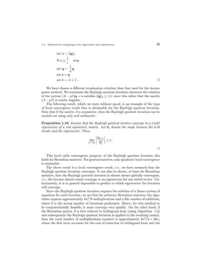
1.4. Methods for computing a few eigenvalues and eigenvectors 39
set α = ‖q‖2
if α ≥ 1ε
stop
set q← 1αq
set s = q
set k ← k + 1 . 2
We have chosen a different termination criterion than that used for the inversepower method. We terminate the Rayleigh quotient iteration whenever the solutionof the system (A − µI)q = s satisfies ‖q‖2 ≥ 1/ε since this infers that the matrix(A− µI) is nearly singular.
The following result, which we state without proof, is an example of the typeof local convergence result that is obtainable for the Rayleigh quotient iteration.Note that if the matrix A is symmetric, then the Rayleigh quotient iteration can becarried out using only real arithmetic.
Proposition 1.16 Assume that the Rayleigh quotient iterates converge to a (real)eigenvector of a real symmetric matrix. Let θk denote the angle between the k-thiterate and the eigenvector. Then,
limk→∞
∣∣∣∣θk+1
θ3k
∣∣∣∣ ≤ 1 .
2
This local cubic convergence property of the Rayleigh quotient iteration alsoholds for Hermitian matrices. For general matrices, only quadratic local convergenceis attainable.
The above result is a local convergence result, i.e., we have assumed that theRayleigh quotient iteration converges. It can also be shown, at least for Hermitianmatrices, that the Rayleigh quotient iteration is almost always globally convergent,i.e., the iterates almost surely converge to an eigenvector for any initial vector. Un-fortunately, it is in general impossible to predict to which eigenvector the iterationwill converge.
Since the Rayleigh quotient iteration requires the solution of a linear system ofequations for each iteration, we see that for arbitrary Hermitian matrices, the algo-rithm requires approximately kn3/6 multiplications and a like number of additions,where k is the actual number of iterations performed. Hence, for this method tobe computationally feasible, it must converge very quickly. On the other hand, ifthe Hermitian matrix A is first reduced to tridiagonal form (using Algorithm 1.2)and subsequently the Rayleigh quotient iteration is applied to the resulting matrix,then the total number of multiplications required is approximately 2n3/3 + 4kn,where the first term accounts for the cost of reduction to tridiagonal form and the
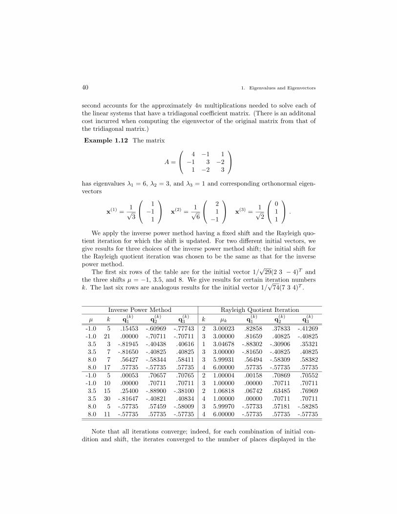
40 1. Eigenvalues and Eigenvectors
second accounts for the approximately 4n multiplications needed to solve each ofthe linear systems that have a tridiagonal coefficient matrix. (There is an additonalcost incurred when computing the eigenvector of the original matrix from that ofthe tridiagonal matrix.)
Example 1.12 The matrix
A =
4 −1 1−1 3 −2
1 −2 3
has eigenvalues λ1 = 6, λ2 = 3, and λ3 = 1 and corresponding orthonormal eigen-vectors
x(1) =1√3
1−1
1
x(2) =1√6
21−1
x(3) =1√2
011
.
We apply the inverse power method having a fixed shift and the Rayleigh quo-tient iteration for which the shift is updated. For two different initial vectors, wegive results for three choices of the inverse power method shift; the initial shift forthe Rayleigh quotient iteration was chosen to be the same as that for the inversepower method.
The first six rows of the table are for the initial vector 1/√
29(2 3 − 4)T andthe three shifts µ = −1, 3.5, and 8. We give results for certain iteration numbersk. The last six rows are analogous results for the initial vector 1/
√74(7 3 4)T .
Inverse Power Method Rayleigh Quotient Iterationµ k q(k)
1 q(k)2 q(k)
3 k µk q(k)1 q(k)
2 q(k)3
-1.0 5 .15453 -.60969 -.77743 2 3.00023 .82858 .37833 -.41269-1.0 21 .00000 -.70711 -.70711 3 3.00000 .81659 .40825 -.408253.5 3 -.81945 -.40438 .40616 1 3.04678 -.88302 -.30906 .353213.5 7 -.81650 -.40825 .40825 3 3.00000 -.81650 -.40825 .408258.0 7 .56427 -.58344 .58411 3 5.99931 .56494 -.58309 .583828.0 17 .57735 -.57735 .57735 4 6.00000 .57735 -.57735 .57735
-1.0 5 .00053 .70657 .70765 2 1.00004 .00158 .70869 .70552-1.0 10 .00000 .70711 .70711 3 1.00000 .00000 .70711 .707113.5 15 .25400 -.88900 -.38100 2 1.06818 .06742 .63485 .769693.5 30 -.81647 -.40821 .40834 4 1.00000 .00000 .70711 .707118.0 5 -.57735 .57459 -.58009 3 5.99970 -.57733 .57181 -.582858.0 11 -.57735 .57735 -.57735 4 6.00000 -.57735 .57735 -.57735
Note that all iterations converge; indeed, for each combination of initial con-dition and shift, the iterates converged to the number of places displayed in the
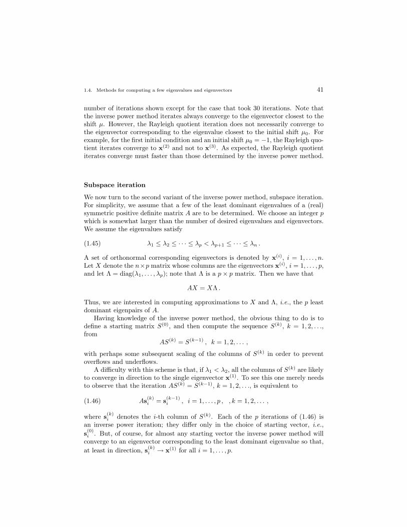
1.4. Methods for computing a few eigenvalues and eigenvectors 41
number of iterations shown except for the case that took 30 iterations. Note thatthe inverse power method iterates always converge to the eigenvector closest to theshift µ. However, the Rayleigh quotient iteration does not necessarily converge tothe eigenvector corresponding to the eigenvalue closest to the initial shift µ0. Forexample, for the first initial condition and an initial shift µ0 = −1, the Rayleigh quo-tient iterates converge to x(2) and not to x(3). As expected, the Rayleigh quotientiterates converge must faster than those determined by the inverse power method.
Subspace iteration
We now turn to the second variant of the inverse power method, subspace iteration.For simplicity, we assume that a few of the least dominant eigenvalues of a (real)symmetric positive definite matrix A are to be determined. We choose an integer pwhich is somewhat larger than the number of desired eigenvalues and eigenvectors.We assume the eigenvalues satisfy
λ1 ≤ λ2 ≤ · · · ≤ λp < λp+1 ≤ · · · ≤ λn .(1.45)
A set of orthonormal corresponding eigenvectors is denoted by x(i), i = 1, . . . , n.Let X denote the n×p matrix whose columns are the eigenvectors x(i), i = 1, . . . , p,and let Λ = diag(λ1, . . . , λp); note that Λ is a p× p matrix. Then we have that
AX = XΛ .
Thus, we are interested in computing approximations to X and Λ, i.e., the p leastdominant eigenpairs of A.
Having knowledge of the inverse power method, the obvious thing to do is todefine a starting matrix S(0), and then compute the sequence S(k), k = 1, 2, . . .,from
AS(k) = S(k−1) , k = 1, 2, . . . ,
with perhaps some subsequent scaling of the columns of S(k) in order to preventoverflows and underflows.
A difficulty with this scheme is that, if λ1 < λ2, all the columns of S(k) are likelyto converge in direction to the single eigenvector x(1). To see this one merely needsto observe that the iteration AS(k) = S(k−1), k = 1, 2, . . ., is equivalent to
As(k)i = s(k−1)
i , i = 1, . . . , p , , k = 1, 2, . . . ,(1.46)
where s(k)i denotes the i-th column of S(k). Each of the p iterations of (1.46) is
an inverse power iteration; they differ only in the choice of starting vector, i.e.,s(0)i . But, of course, for almost any starting vector the inverse power method will
converge to an eigenvector corresponding to the least dominant eigenvalue so that,at least in direction, s(k)
i → x(1) for all i = 1, . . . , p.
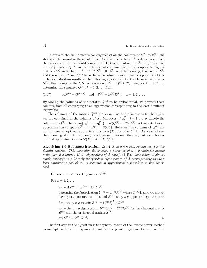
42 1. Eigenvalues and Eigenvectors
To prevent the simultaneous convergence of all the columns of S(k) to x(1), oneshould orthonormalize these columns. For example, after S(k) is determined fromthe previous iterate, we could compute the QR factorization of S(k), i.e., determinean n × p matrix Q(k) having orthonormal columns and a p × p upper triangularmatrix R(k) such that S(k) = Q(k)R(k). If S(k) is of full rank p, then so is R(k)
and therefore S(k) and Q(k) have the same column space. The incorporation of thisorthonormalization results in the following algorithm. Start with an initial matrixS(0); then compute the QR factorization S(0) = Q(0)R(0); then, for k = 1, 2, . . . ,determine the sequence Q(k), k = 1, 2, . . ., from
AS(k) = Q(k−1) and S(k) = Q(k)R(k) , k = 1, 2, . . . .(1.47)
By forcing the columns of the iterates Q(k) to be orthonormal, we prevent thesecolumns from all converging to an eigenvector corresponding to the least dominanteigenvalue.
The columns of the matrix Q(k) are viewed as approximations to the eigen-vectors contained in the columns of X. Moreover, if q(k)
i , i = 1, . . . , p, denote thecolumns of Q(k), then span{q(k)
1 , . . . ,q(k)p } = R(Q(k)) = R(S(k)) is thought of as an
approximation to span{x(1), . . . ,x(p)} = R(X). However, the columns of Q(k) arenot, in general, optimal approximations to R(X) out of R(Q(k)). As we shall see,the following algorithm not only produces orthonormal iterates, but also choosesoptimal approximations to R(X) out of R(Q(k)).
Algorithm 1.6 Subspace iteration. Let A be an n×n real, symmetric, positivedefinite matrix. This algorithm determines a sequence of n × p matrices havingorthonormal columns. If the eigenvalues of A satisfy (1.45), these columns almostsurely converge to p linearly independent eigenvectors of A corresponding to the pleast dominant eigenvalues. A sequence of approximate eigenvalues is also gener-ated.
Choose an n× p starting matrix S(0).
For k = 1, 2, . . . ,
solve AY (k) = S(k−1) for Y (k)
determine the factorization Y (k) = Q(k)R(k) where Q(k) is an n×p matrixhaving orthonormal columns and R(k) is a p× p upper triangular matrix
form the p× p matrix B(k) =(Q(k)
)TAQ(k)
solve the p× p eigensystem B(k)Z(k) = Z(k)Θ(k) for the diagonal matrixΘ(k) and the orthogonal matrix Z(k)
set S(k) = Q(k)Z(k). 2
The first step in the algorithm is the generalization of the inverse power methodto multiple vectors. It requires the solution of p linear systems for the columns
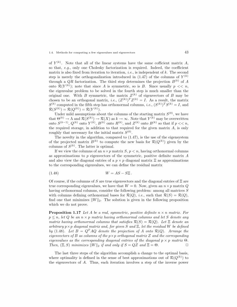
1.4. Methods for computing a few eigenvalues and eigenvectors 43
of Y (k). Note that all of the linear systems have the same cofficient matrix A,so that, e.g., only one Cholesky factorization is required. Indeed, the coefficientmatrix is also fixed from iteration to iteration, i.e., is independent of k. The secondstep is merely the orthogonalization introduced in (1.47) of the columns of Y (k)
through a QR factorization. The third step determines the projection B(k) of Aonto R(Y (k)); note that since A is symmetric, so is B. Since usually p << n,the eigenvalue problem to be solved in the fourth step is much smaller than theoriginal one. With B symmetric, the matrix Z(k) of eigenvectors of B may bechosen to be an orthogonal matrix, i.e., (Z(k))T Z(k) = I. As a result, the matrixS(k) computed in the fifth step has orthonormal columns, i.e., (S(k))T S(k) = I, andR(S(k)) = R(Q(k)) = R(Y (k)).
Under mild assumptions about the columns of the starting matrix S(0), we havethat Θ(k) → Λ and R(S(k))→ R(X) as k →∞. Note that Y (k) may be overwrittenonto S(k−1), Q(k) onto Y (k), B(k) onto R(k), and Z(k) onto B(k) so that if p << n,the required storage, in addition to that required for the given matrix A, is onlyroughly that necessary for the initial matrix S(0).
The novelty in the algorithm, compared to (1.47), is the use of the eigensystemof the projected matrix B(k) to compute the new basis for R(Q(k)) given by thecolumns of S(k). The latter is optimal.
If we view the columns of an n×p matrix S, p < n, having orthonormal columnsas approximations to p eigenvectors of the symmetric, positive definite matrix Aand also view the diagonal entries of a p× p diagonal matrix Ξ as approximationsto the corresponding eigenvalues, we can define the residual matrix
W = AS − SΞ .(1.48)
Of course, if the columns of S are true eigenvectors and the diagonal entries of Ξ aretrue corresponding eigenvalues, we have that W = 0. Now, given an n×p matrix Qhaving orthonormal columns, consider the following problem: among all matrices Swith columns defining orthonormal bases for R(Q), i.e., such that R(S) = R(Q),find one that minimizes ‖W‖2. The solution is given in the following propositionwhich we do not prove.
Proposition 1.17 Let A be a real, symmetric, positive definite n× n matrix. Forp ≤ n, let Q be an n× p matrix having orthonormal columns and let S denote anymatrix having orthonormal columns that satisfies R(S) = R(Q). Let Ξ denote anarbitrary p×p diagonal matrix and, for given S and Ξ, let the residual W be definedby (1.48). Let B = QT AQ denote the projection of A onto R(Q). Arrange theeigenvectors of B as columns of the p×p orthogonal matrix Z and the correspondingeigenvalues as the corresponding diagonal entries of the diagonal p × p matrix Θ.Then, (Ξ, S) minimizes ‖W‖2 if and only if S = QZ and Ξ = Θ. 2
The last three steps of the algorithm accomplish a change to the optimal basis,where optimality is defined in the sense of best approximations out of R(Q(k)) tothe eigenvectors of A. Thus, each iteration involves a step of the inverse power
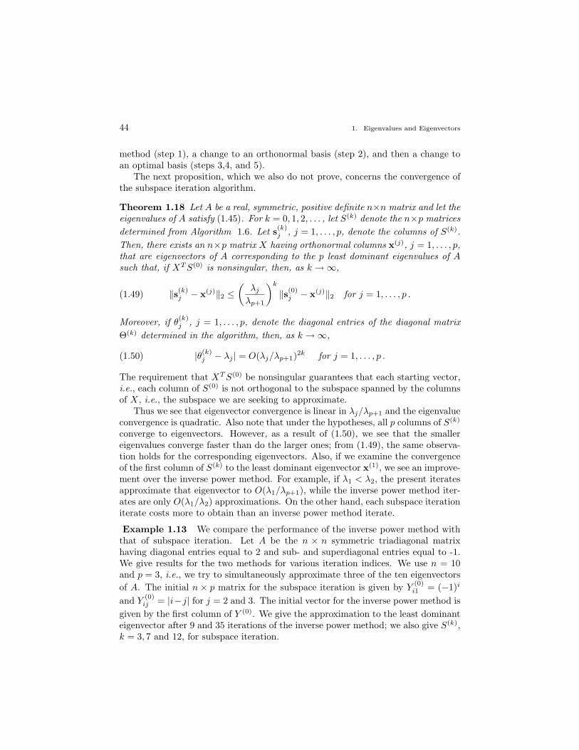
44 1. Eigenvalues and Eigenvectors
method (step 1), a change to an orthonormal basis (step 2), and then a change toan optimal basis (steps 3,4, and 5).
The next proposition, which we also do not prove, concerns the convergence ofthe subspace iteration algorithm.
Theorem 1.18 Let A be a real, symmetric, positive definite n×n matrix and let theeigenvalues of A satisfy (1.45). For k = 0, 1, 2, . . . , let S(k) denote the n×p matricesdetermined from Algorithm 1.6. Let s(k)
j , j = 1, . . . , p, denote the columns of S(k).Then, there exists an n×p matrix X having orthonormal columns x(j), j = 1, . . . , p,that are eigenvectors of A corresponding to the p least dominant eigenvalues of Asuch that, if XT S(0) is nonsingular, then, as k →∞,
‖s(k)j − x(j)‖2 ≤
(λj
λp+1
)k
‖s(0)j − x(j)‖2 for j = 1, . . . , p .(1.49)
Moreover, if θ(k)j , j = 1, . . . , p, denote the diagonal entries of the diagonal matrix
Θ(k) determined in the algorithm, then, as k →∞,
|θ(k)j − λj | = O(λj/λp+1)2k for j = 1, . . . , p .(1.50)
The requirement that XT S(0) be nonsingular guarantees that each starting vector,i.e., each column of S(0) is not orthogonal to the subspace spanned by the columnsof X, i.e., the subspace we are seeking to approximate.
Thus we see that eigenvector convergence is linear in λj/λp+1 and the eigenvalueconvergence is quadratic. Also note that under the hypotheses, all p columns of S(k)
converge to eigenvectors. However, as a result of (1.50), we see that the smallereigenvalues converge faster than do the larger ones; from (1.49), the same observa-tion holds for the corresponding eigenvectors. Also, if we examine the convergenceof the first column of S(k) to the least dominant eigenvector x(1), we see an improve-ment over the inverse power method. For example, if λ1 < λ2, the present iteratesapproximate that eigenvector to O(λ1/λp+1), while the inverse power method iter-ates are only O(λ1/λ2) approximations. On the other hand, each subspace iterationiterate costs more to obtain than an inverse power method iterate.
Example 1.13 We compare the performance of the inverse power method withthat of subspace iteration. Let A be the n × n symmetric triadiagonal matrixhaving diagonal entries equal to 2 and sub- and superdiagonal entries equal to -1.We give results for the two methods for various iteration indices. We use n = 10and p = 3, i.e., we try to simultaneously approximate three of the ten eigenvectorsof A. The initial n × p matrix for the subspace iteration is given by Y
(0)i1 = (−1)i
and Y(0)ij = |i−j| for j = 2 and 3. The initial vector for the inverse power method is
given by the first column of Y (0). We give the approximation to the least dominanteigenvector after 9 and 35 iterations of the inverse power method; we also give S(k),k = 3, 7 and 12, for subspace iteration.
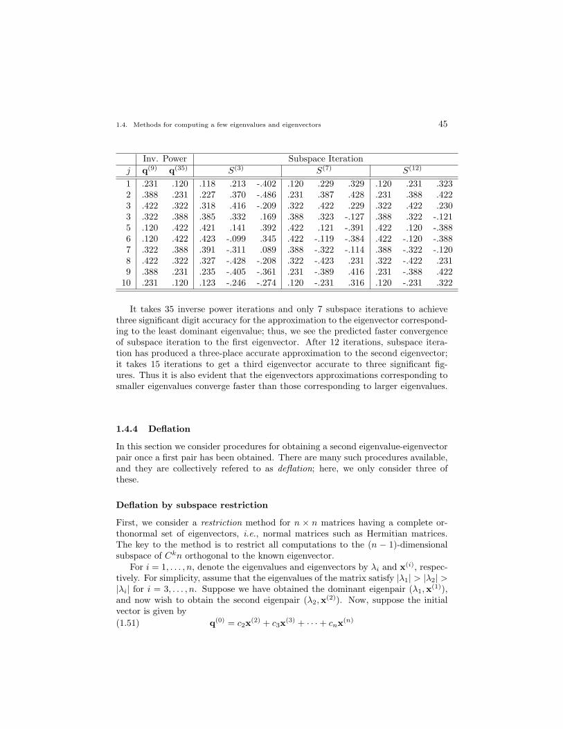
1.4. Methods for computing a few eigenvalues and eigenvectors 45
Inv. Power Subspace Iterationj q(9) q(35) S(3) S(7) S(12)
1 .231 .120 .118 .213 -.402 .120 .229 .329 .120 .231 .3232 .388 .231 .227 .370 -.486 .231 .387 .428 .231 .388 .4223 .422 .322 .318 .416 -.209 .322 .422 .229 .322 .422 .2303 .322 .388 .385 .332 .169 .388 .323 -.127 .388 .322 -.1215 .120 .422 .421 .141 .392 .422 .121 -.391 .422 .120 -.3886 .120 .422 .423 -.099 .345 .422 -.119 -.384 .422 -.120 -.3887 .322 .388 .391 -.311 .089 .388 -.322 -.114 .388 -.322 -.1208 .422 .322 .327 -.428 -.208 .322 -.423 .231 .322 -.422 .2319 .388 .231 .235 -.405 -.361 .231 -.389 .416 .231 -.388 .422
10 .231 .120 .123 -.246 -.274 .120 -.231 .316 .120 -.231 .322
It takes 35 inverse power iterations and only 7 subspace iterations to achievethree significant digit accuracy for the approximation to the eigenvector correspond-ing to the least dominant eigenvalue; thus, we see the predicted faster convergenceof subspace iteration to the first eigenvector. After 12 iterations, subspace itera-tion has produced a three-place accurate approximation to the second eigenvector;it takes 15 iterations to get a third eigenvector accurate to three significant fig-ures. Thus it is also evident that the eigenvectors approximations corresponding tosmaller eigenvalues converge faster than those corresponding to larger eigenvalues.
1.4.4 Deflation
In this section we consider procedures for obtaining a second eigenvalue-eigenvectorpair once a first pair has been obtained. There are many such procedures available,and they are collectively refered to as deflation; here, we only consider three ofthese.
Deflation by subspace restriction
First, we consider a restriction method for n × n matrices having a complete or-thonormal set of eigenvectors, i.e., normal matrices such as Hermitian matrices.The key to the method is to restrict all computations to the (n − 1)-dimensionalsubspace of Ckn orthogonal to the known eigenvector.
For i = 1, . . . , n, denote the eigenvalues and eigenvectors by λi and x(i), respec-tively. For simplicity, assume that the eigenvalues of the matrix satisfy |λ1| > |λ2| >|λi| for i = 3, . . . , n. Suppose we have obtained the dominant eigenpair (λ1,x(1)),and now wish to obtain the second eigenpair (λ2,x(2)). Now, suppose the initialvector is given by
q(0) = c2x(2) + c3x(3) + · · ·+ cnx(n)(1.51)
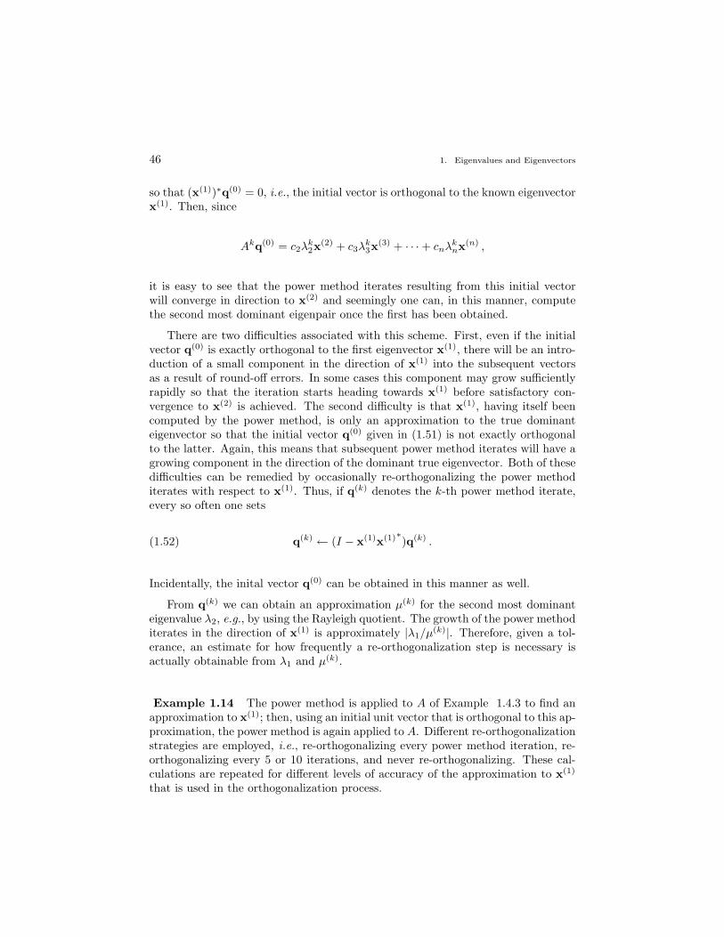
46 1. Eigenvalues and Eigenvectors
so that (x(1))∗q(0) = 0, i.e., the initial vector is orthogonal to the known eigenvectorx(1). Then, since
Akq(0) = c2λk2x
(2) + c3λk3x
(3) + · · ·+ cnλknx(n) ,
it is easy to see that the power method iterates resulting from this initial vectorwill converge in direction to x(2) and seemingly one can, in this manner, computethe second most dominant eigenpair once the first has been obtained.
There are two difficulties associated with this scheme. First, even if the initialvector q(0) is exactly orthogonal to the first eigenvector x(1), there will be an intro-duction of a small component in the direction of x(1) into the subsequent vectorsas a result of round-off errors. In some cases this component may grow sufficientlyrapidly so that the iteration starts heading towards x(1) before satisfactory con-vergence to x(2) is achieved. The second difficulty is that x(1), having itself beencomputed by the power method, is only an approximation to the true dominanteigenvector so that the initial vector q(0) given in (1.51) is not exactly orthogonalto the latter. Again, this means that subsequent power method iterates will have agrowing component in the direction of the dominant true eigenvector. Both of thesedifficulties can be remedied by occasionally re-orthogonalizing the power methoditerates with respect to x(1). Thus, if q(k) denotes the k-th power method iterate,every so often one sets
q(k) ← (I − x(1)x(1)∗)q(k) .(1.52)
Incidentally, the inital vector q(0) can be obtained in this manner as well.
From q(k) we can obtain an approximation µ(k) for the second most dominanteigenvalue λ2, e.g., by using the Rayleigh quotient. The growth of the power methoditerates in the direction of x(1) is approximately |λ1/µ(k)|. Therefore, given a tol-erance, an estimate for how frequently a re-orthogonalization step is necessary isactually obtainable from λ1 and µ(k).
Example 1.14 The power method is applied to A of Example 1.4.3 to find anapproximation to x(1); then, using an initial unit vector that is orthogonal to this ap-proximation, the power method is again applied to A. Different re-orthogonalizationstrategies are employed, i.e., re-orthogonalizing every power method iteration, re-orthogonalizing every 5 or 10 iterations, and never re-orthogonalizing. These cal-culations are repeated for different levels of accuracy of the approximation to x(1)
that is used in the orthogonalization process.
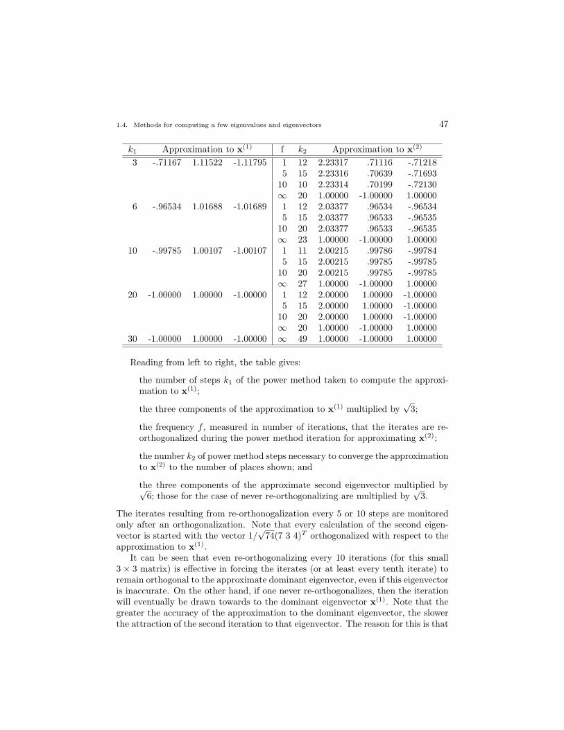
1.4. Methods for computing a few eigenvalues and eigenvectors 47
k1 Approximation to x(1) f k2 Approximation to x(2)
3 -.71167 1.11522 -1.11795 1 12 2.23317 .71116 -.712185 15 2.23316 .70639 -.71693
10 10 2.23314 .70199 -.72130∞ 20 1.00000 -1.00000 1.00000
6 -.96534 1.01688 -1.01689 1 12 2.03377 .96534 -.965345 15 2.03377 .96533 -.96535
10 20 2.03377 .96533 -.96535∞ 23 1.00000 -1.00000 1.00000
10 -.99785 1.00107 -1.00107 1 11 2.00215 .99786 -.997845 15 2.00215 .99785 -.99785
10 20 2.00215 .99785 -.99785∞ 27 1.00000 -1.00000 1.00000
20 -1.00000 1.00000 -1.00000 1 12 2.00000 1.00000 -1.000005 15 2.00000 1.00000 -1.00000
10 20 2.00000 1.00000 -1.00000∞ 20 1.00000 -1.00000 1.00000
30 -1.00000 1.00000 -1.00000 ∞ 49 1.00000 -1.00000 1.00000
Reading from left to right, the table gives:
the number of steps k1 of the power method taken to compute the approxi-mation to x(1);
the three components of the approximation to x(1) multiplied by√
3;
the frequency f , measured in number of iterations, that the iterates are re-orthogonalized during the power method iteration for approximating x(2);
the number k2 of power method steps necessary to converge the approximationto x(2) to the number of places shown; and
the three components of the approximate second eigenvector multiplied by√6; those for the case of never re-orthogonalizing are multiplied by
√3.
The iterates resulting from re-orthonogalization every 5 or 10 steps are monitoredonly after an orthogonalization. Note that every calculation of the second eigen-vector is started with the vector 1/
√74(7 3 4)T orthogonalized with respect to the
approximation to x(1).It can be seen that even re-orthogonalizing every 10 iterations (for this small
3 × 3 matrix) is effective in forcing the iterates (or at least every tenth iterate) toremain orthogonal to the approximate dominant eigenvector, even if this eigenvectoris inaccurate. On the other hand, if one never re-orthogonalizes, then the iterationwill eventually be drawn towards to the dominant eigenvector x(1). Note that thegreater the accuracy of the approximation to the dominant eigenvector, the slowerthe attraction of the second iteration to that eigenvector. The reason for this is that
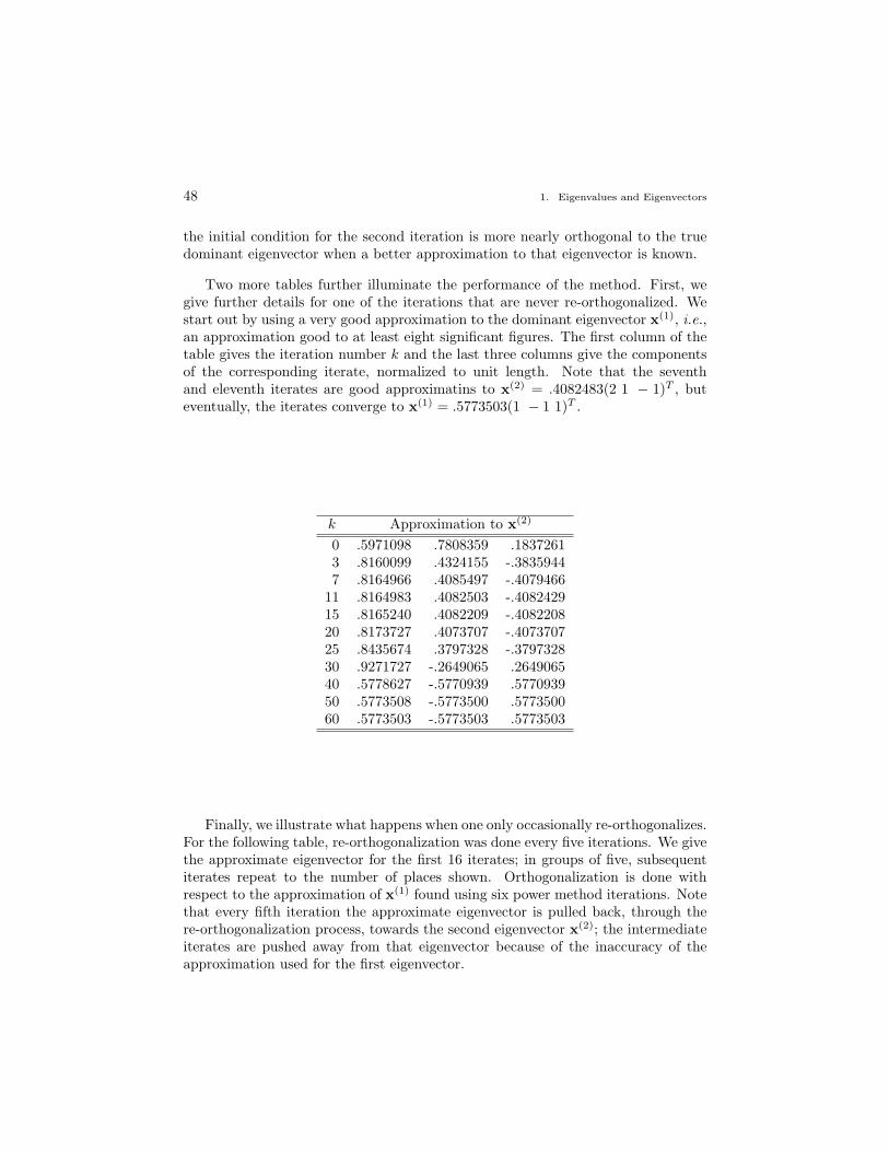
48 1. Eigenvalues and Eigenvectors
the initial condition for the second iteration is more nearly orthogonal to the truedominant eigenvector when a better approximation to that eigenvector is known.
Two more tables further illuminate the performance of the method. First, wegive further details for one of the iterations that are never re-orthogonalized. Westart out by using a very good approximation to the dominant eigenvector x(1), i.e.,an approximation good to at least eight significant figures. The first column of thetable gives the iteration number k and the last three columns give the componentsof the corresponding iterate, normalized to unit length. Note that the seventhand eleventh iterates are good approximatins to x(2) = .4082483(2 1 − 1)T , buteventually, the iterates converge to x(1) = .5773503(1 − 1 1)T .
k Approximation to x(2)
0 .5971098 .7808359 .18372613 .8160099 .4324155 -.38359447 .8164966 .4085497 -.4079466
11 .8164983 .4082503 -.408242915 .8165240 .4082209 -.408220820 .8173727 .4073707 -.407370725 .8435674 .3797328 -.379732830 .9271727 -.2649065 .264906540 .5778627 -.5770939 .577093950 .5773508 -.5773500 .577350060 .5773503 -.5773503 .5773503
Finally, we illustrate what happens when one only occasionally re-orthogonalizes.For the following table, re-orthogonalization was done every five iterations. We givethe approximate eigenvector for the first 16 iterates; in groups of five, subsequentiterates repeat to the number of places shown. Orthogonalization is done withrespect to the approximation of x(1) found using six power method iterations. Notethat every fifth iteration the approximate eigenvector is pulled back, through there-orthogonalization process, towards the second eigenvector x(2); the intermediateiterates are pushed away from that eigenvector because of the inaccuracy of theapproximation used for the first eigenvector.
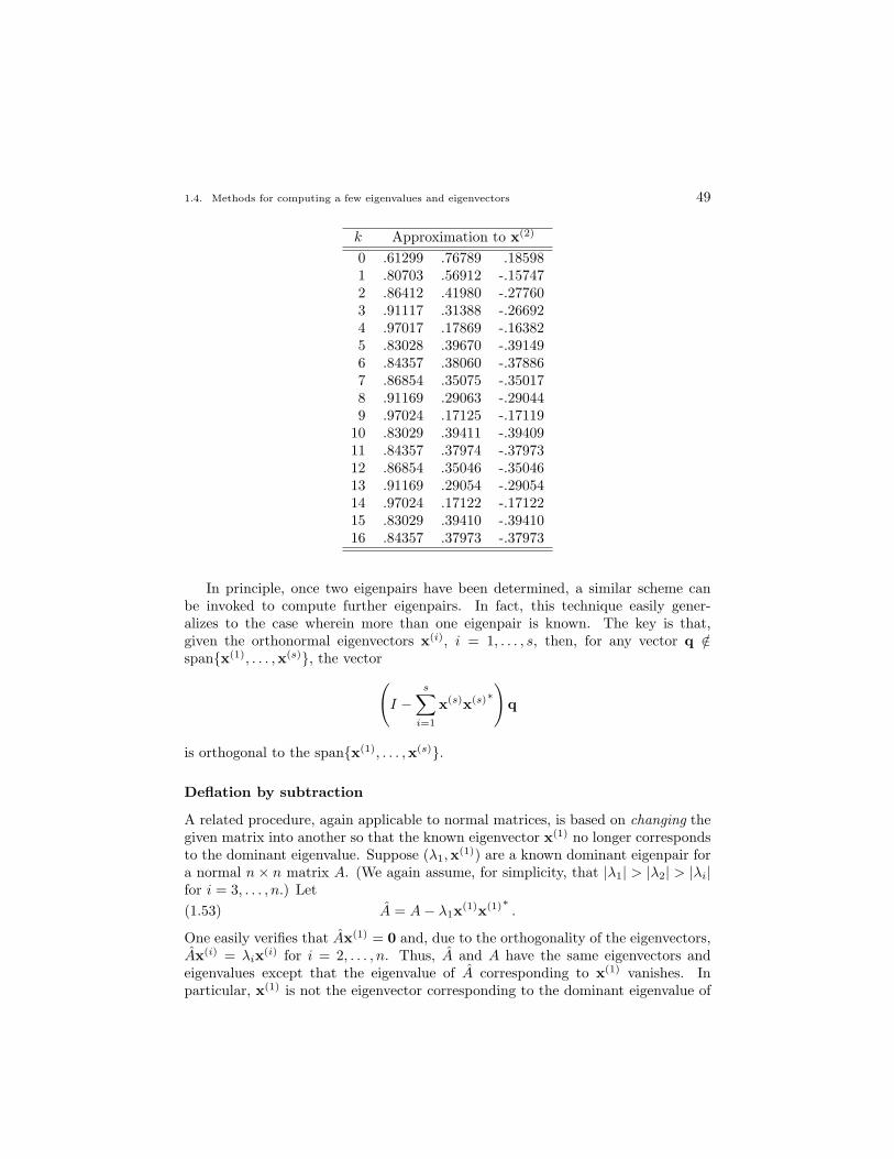
1.4. Methods for computing a few eigenvalues and eigenvectors 49
k Approximation to x(2)
0 .61299 .76789 .185981 .80703 .56912 -.157472 .86412 .41980 -.277603 .91117 .31388 -.266924 .97017 .17869 -.163825 .83028 .39670 -.391496 .84357 .38060 -.378867 .86854 .35075 -.350178 .91169 .29063 -.290449 .97024 .17125 -.17119
10 .83029 .39411 -.3940911 .84357 .37974 -.3797312 .86854 .35046 -.3504613 .91169 .29054 -.2905414 .97024 .17122 -.1712215 .83029 .39410 -.3941016 .84357 .37973 -.37973
In principle, once two eigenpairs have been determined, a similar scheme canbe invoked to compute further eigenpairs. In fact, this technique easily gener-alizes to the case wherein more than one eigenpair is known. The key is that,given the orthonormal eigenvectors x(i), i = 1, . . . , s, then, for any vector q /∈span{x(1), . . . ,x(s)}, the vector(
I −s∑
i=1
x(s)x(s)∗)
q
is orthogonal to the span{x(1), . . . ,x(s)}.
Deflation by subtraction
A related procedure, again applicable to normal matrices, is based on changing thegiven matrix into another so that the known eigenvector x(1) no longer correspondsto the dominant eigenvalue. Suppose (λ1,x(1)) are a known dominant eigenpair fora normal n× n matrix A. (We again assume, for simplicity, that |λ1| > |λ2| > |λi|for i = 3, . . . , n.) Let
A = A− λ1x(1)x(1)∗ .(1.53)
One easily verifies that Ax(1) = 0 and, due to the orthogonality of the eigenvectors,Ax(i) = λix(i) for i = 2, . . . , n. Thus, A and A have the same eigenvectors andeigenvalues except that the eigenvalue of A corresponding to x(1) vanishes. Inparticular, x(1) is not the eigenvector corresponding to the dominant eigenvalue of
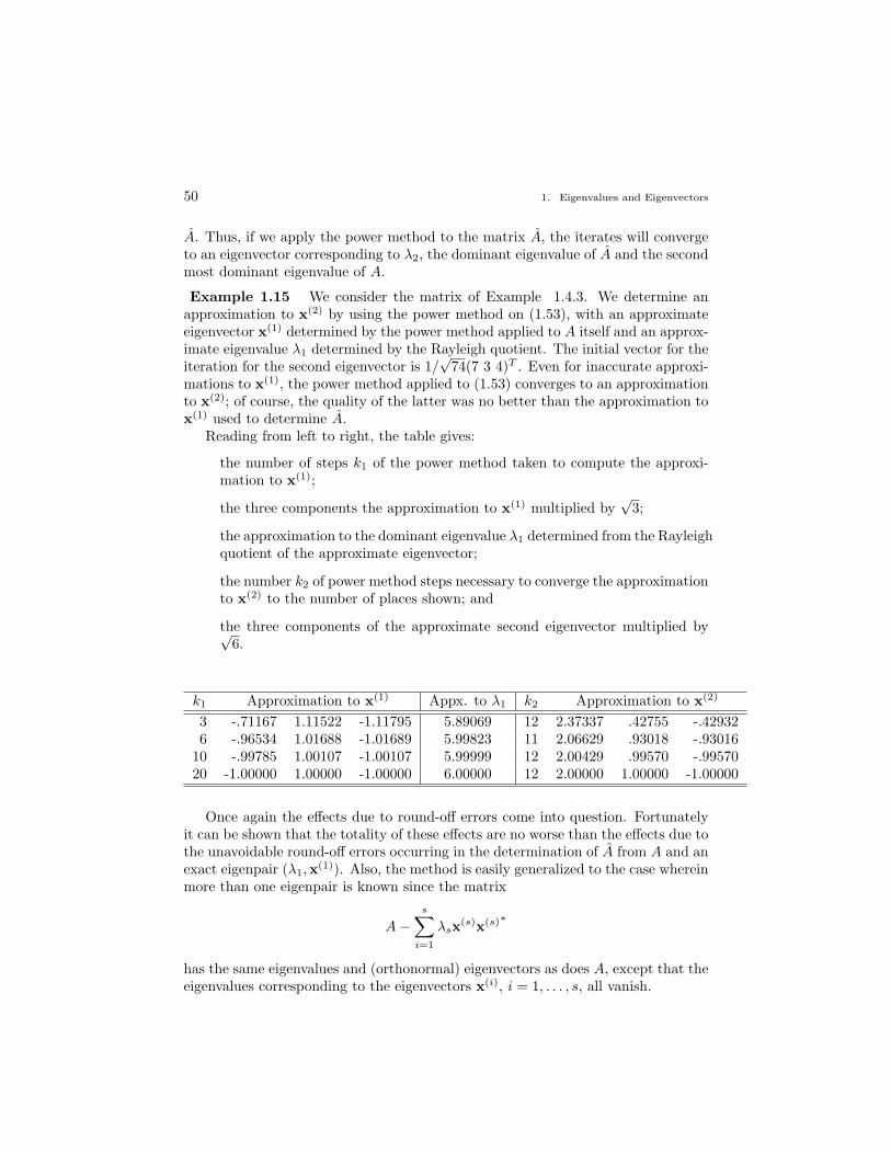
50 1. Eigenvalues and Eigenvectors
A. Thus, if we apply the power method to the matrix A, the iterates will convergeto an eigenvector corresponding to λ2, the dominant eigenvalue of A and the secondmost dominant eigenvalue of A.
Example 1.15 We consider the matrix of Example 1.4.3. We determine anapproximation to x(2) by using the power method on (1.53), with an approximateeigenvector x(1) determined by the power method applied to A itself and an approx-imate eigenvalue λ1 determined by the Rayleigh quotient. The initial vector for theiteration for the second eigenvector is 1/
√74(7 3 4)T . Even for inaccurate approxi-
mations to x(1), the power method applied to (1.53) converges to an approximationto x(2); of course, the quality of the latter was no better than the approximation tox(1) used to determine A.
Reading from left to right, the table gives:
the number of steps k1 of the power method taken to compute the approxi-mation to x(1);
the three components the approximation to x(1) multiplied by√
3;
the approximation to the dominant eigenvalue λ1 determined from the Rayleighquotient of the approximate eigenvector;
the number k2 of power method steps necessary to converge the approximationto x(2) to the number of places shown; and
the three components of the approximate second eigenvector multiplied by√6.
k1 Approximation to x(1) Appx. to λ1 k2 Approximation to x(2)
3 -.71167 1.11522 -1.11795 5.89069 12 2.37337 .42755 -.429326 -.96534 1.01688 -1.01689 5.99823 11 2.06629 .93018 -.93016
10 -.99785 1.00107 -1.00107 5.99999 12 2.00429 .99570 -.9957020 -1.00000 1.00000 -1.00000 6.00000 12 2.00000 1.00000 -1.00000
Once again the effects due to round-off errors come into question. Fortunatelyit can be shown that the totality of these effects are no worse than the effects due tothe unavoidable round-off errors occurring in the determination of A from A and anexact eigenpair (λ1,x(1)). Also, the method is easily generalized to the case whereinmore than one eigenpair is known since the matrix
A−s∑
i=1
λsx(s)x(s)∗
has the same eigenvalues and (orthonormal) eigenvectors as does A, except that theeigenvalues corresponding to the eigenvectors x(i), i = 1, . . . , s, all vanish.
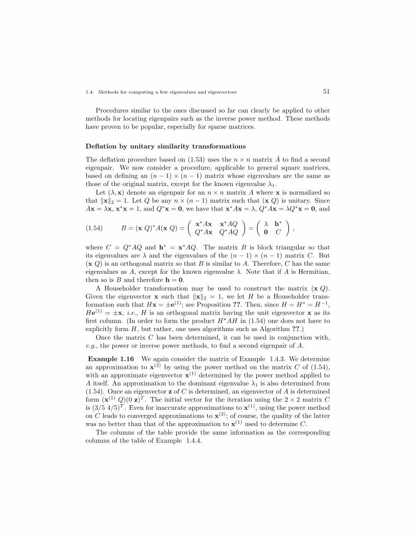
1.4. Methods for computing a few eigenvalues and eigenvectors 51
Procedures similar to the ones discussed so far can clearly be applied to othermethods for locating eigenpairs such as the inverse power method. These methodshave proven to be popular, especially for sparse matrices.
Deflation by unitary similarity transformations
The deflation procedure based on (1.53) uses the n × n matrix A to find a secondeigenpair. We now consider a procedure, applicable to general square matrices,based on defining an (n − 1) × (n − 1) matrix whose eigenvalues are the same asthose of the original matrix, except for the known eigenvalue λ1.
Let (λ,x) denote an eigenpair for an n × n matrix A where x is normalized sothat ‖x‖2 = 1. Let Q be any n× (n− 1) matrix such that (x Q) is unitary. SinceAx = λx, x∗x = 1, and Q∗x = 0, we have that x∗Ax = λ, Q∗Ax = λQ∗x = 0, and
B = (x Q)∗A(x Q) =(
x∗Ax x∗AQQ∗Ax Q∗AQ
)=(
λ h∗
0 C
),(1.54)
where C = Q∗AQ and h∗ = x∗AQ. The matrix B is block triangular so thatits eigenvalues are λ and the eigenvalues of the (n − 1) × (n − 1) matrix C. But(x Q) is an orthogonal matrix so that B is similar to A. Therefore, C has the sameeigenvalues as A, except for the known eigenvalue λ. Note that if A is Hermitian,then so is B and therefore h = 0.
A Householder transformation may be used to construct the matrix (x Q).Given the eigenvector x such that ‖x‖2 = 1, we let H be a Householder trans-formation such that Hx = ±e(1); see Proposition ??. Then, since H = H∗ = H−1,He(1) = ±x, i.e., H is an orthogonal matrix having the unit eigenvector x as itsfirst column. (In order to form the product H∗AH in (1.54) one does not have toexplicitly form H, but rather, one uses algorithms such as Algorithm ??.)
Once the matrix C has been determined, it can be used in conjunction with,e.g., the power or inverse power methods, to find a second eigenpair of A.
Example 1.16 We again consider the matrix of Example 1.4.3. We determinean approximation to x(2) by using the power method on the matrix C of (1.54),with an approximate eigenvector x(1) determined by the power method applied toA itself. An approximation to the dominant eigenvalue λ1 is also determined from(1.54). Once an eigenvector z of C is determined, an eigenvector of A is determinedform (x(1) Q)(0 z)T . The initial vector for the iteration using the 2 × 2 matrix Cis (3/5 4/5)T . Even for inaccurate approximations to x(1), using the power methodon C leads to converged approximations to x(2); of course, the quality of the latterwas no better than that of the approximation to x(1) used to determine C.
The columns of the table provide the same information as the correspondingcolumns of the table of Example 1.4.4.
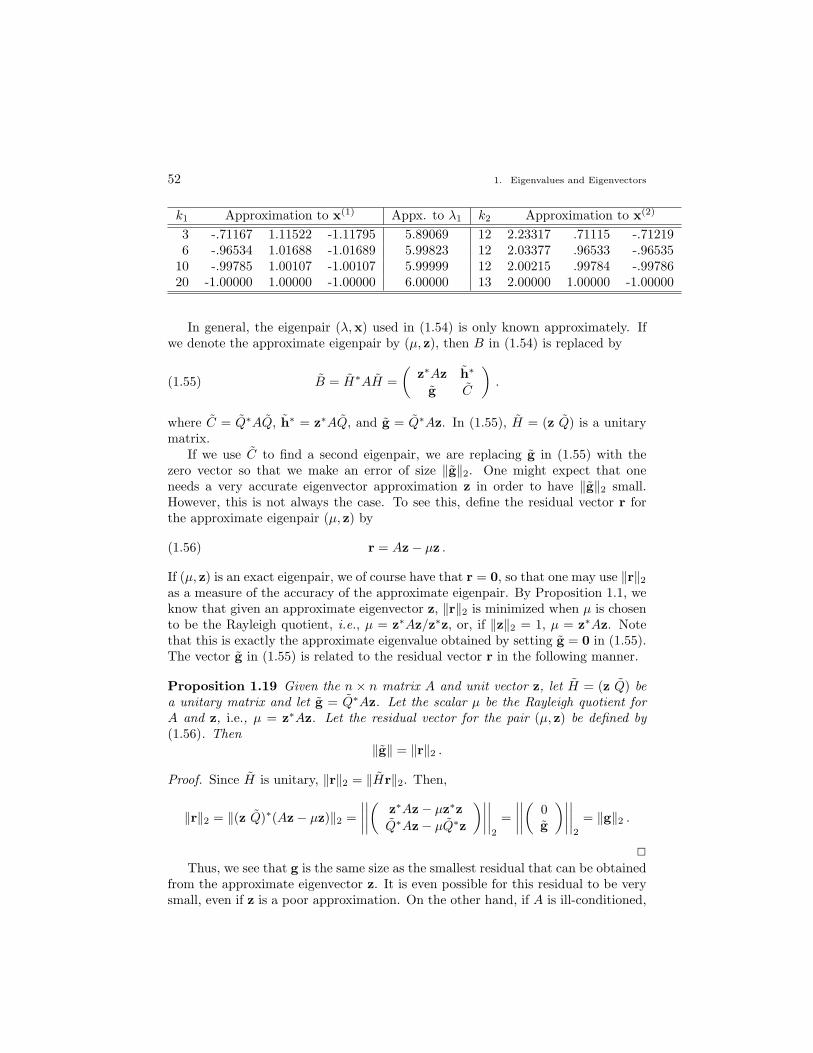
52 1. Eigenvalues and Eigenvectors
k1 Approximation to x(1) Appx. to λ1 k2 Approximation to x(2)
3 -.71167 1.11522 -1.11795 5.89069 12 2.23317 .71115 -.712196 -.96534 1.01688 -1.01689 5.99823 12 2.03377 .96533 -.96535
10 -.99785 1.00107 -1.00107 5.99999 12 2.00215 .99784 -.9978620 -1.00000 1.00000 -1.00000 6.00000 13 2.00000 1.00000 -1.00000
In general, the eigenpair (λ,x) used in (1.54) is only known approximately. Ifwe denote the approximate eigenpair by (µ, z), then B in (1.54) is replaced by
B = H∗AH =(
z∗Az h∗
g C
).(1.55)
where C = Q∗AQ, h∗ = z∗AQ, and g = Q∗Az. In (1.55), H = (z Q) is a unitarymatrix.
If we use C to find a second eigenpair, we are replacing g in (1.55) with thezero vector so that we make an error of size ‖g‖2. One might expect that oneneeds a very accurate eigenvector approximation z in order to have ‖g‖2 small.However, this is not always the case. To see this, define the residual vector r forthe approximate eigenpair (µ, z) by
r = Az− µz .(1.56)
If (µ, z) is an exact eigenpair, we of course have that r = 0, so that one may use ‖r‖2as a measure of the accuracy of the approximate eigenpair. By Proposition 1.1, weknow that given an approximate eigenvector z, ‖r‖2 is minimized when µ is chosento be the Rayleigh quotient, i.e., µ = z∗Az/z∗z, or, if ‖z‖2 = 1, µ = z∗Az. Notethat this is exactly the approximate eigenvalue obtained by setting g = 0 in (1.55).The vector g in (1.55) is related to the residual vector r in the following manner.
Proposition 1.19 Given the n× n matrix A and unit vector z, let H = (z Q) bea unitary matrix and let g = Q∗Az. Let the scalar µ be the Rayleigh quotient forA and z, i.e., µ = z∗Az. Let the residual vector for the pair (µ, z) be defined by(1.56). Then
‖g‖ = ‖r‖2 .
Proof. Since H is unitary, ‖r‖2 = ‖Hr‖2. Then,
‖r‖2 = ‖(z Q)∗(Az− µz)‖2 =∣∣∣∣∣∣∣∣( z∗Az− µz∗z
Q∗Az− µQ∗z
)∣∣∣∣∣∣∣∣2
=∣∣∣∣∣∣∣∣( 0
g
)∣∣∣∣∣∣∣∣2
= ‖g‖2 .
2
Thus, we see that g is the same size as the smallest residual that can be obtainedfrom the approximate eigenvector z. It is even possible for this residual to be verysmall, even if z is a poor approximation. On the other hand, if A is ill-conditioned,
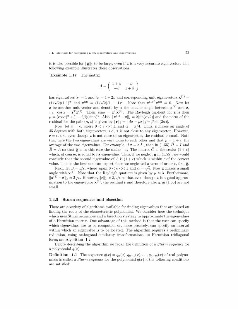
1.4. Methods for computing a few eigenvalues and eigenvectors 53
it is also possible for ‖g‖2 to be large, even if z is a very accurate eigenvector. Thefollowing example illustrates these observations.
Example 1.17 The matrix
A =(
1 + β −β−β 1 + β
)has eigenvalues λ1 = 1 and λ2 = 1 + 2β and corresponding unit eigenvectors x(1) =(1/√
2)(1 1)T and x(2) = (1/√
2)(1 − 1)T . Note that x(1)Tx(2) = 0. Now let
z be another unit vector and denote by α the smaller angle between x(1) and z,i.e., cosα = zT x(1). Then, sinα = zT x(2). The Rayleigh quotient for z is thenµ = (cosα)2 + (1 + 2β)(sinα)2. Also, ‖x(1) − z‖2 = 2|sin(α/2)| and the norm of theresidual for the pair (µ, z) is given by ‖r‖2 = ‖Az− µz‖2 = β|sin(2α)|.
Now, let β = ε, where 0 < ε << 1, and α = π/4. Thus, z makes an angle of45 degrees with both eigenvectors, i.e., z is not close to any eigenvector. However,r = ε, i.e., even though z is not close to an eigenvector, the residual is small. Notethat here the two eigenvalues are very close to each other and that µ = 1 + ε, theaverage of the two eigenvalues. For example, if z = e(1), then in (1.55) H = I andB = A so that g is in this case the scalar −ε. The matrix C is the scalar (1 + ε)which, of course, is equal to its eigenvalue. Thus, if we neglect g in (1.55), we wouldconclude that the second eigenvalue of A is (1 + ε) which is within ε of the correctvalue. This is the best one can expect since we neglected a term of order ε, i.e., g.
Next, let β = 1/ε, where again 0 < ε << 1 and α =√
ε. Now z makes a smallangle with x(1). Note that the Rayleigh quotient is given by µ ≈ 3. Furthermore,‖x(1) − z‖2 ≈ 2
√ε. However, ‖r‖2 ≈ 2/
√ε so that even though z is a good approx-
imation to the eigenvector x(1), the residual r and therefore also g in (1.55) are notsmall.
1.4.5 Sturm sequences and bisection
There are a variety of algorithms available for finding eigenvalues that are based onfinding the roots of the characteristic polynomial. We consider here the techniquewhich uses Sturm sequences and a bisection strategy to approximate the eigenvaluesof a Hermitian matrix. One advantage of this method is that the user can specifywhich eigenvalues are to be computed, or, more precisely, can specify an intervalwithin which an eigenvalue is to be located. The algorithm requires a preliminaryreduction, using orthogonal similarity transformations, to Hermitian tridiagonalform; see Algorithm 1.2.
Before describing the algorithm we recall the definition of a Sturm sequence fora polynomial q(x).Definition 1.1 The sequence q(x) = qn(x), qn−1(x), . . . , qn−m(x) of real polyno-mials is called a Sturm sequence for the polynomial q(x) if the following conditionsare satisfied:
54 1. Eigenvalues and Eigenvectors
i. the real roots of q(x) = qn(x) are simple;
ii. if η is a real root of q(x) = qn(x), then sign qn−1(η) = −sign q′n(η) ;
iii. if η is a real root of qi(x), then, for i = n−1, n−2, . . . , n−m+1, qi+1(η)qi−1(η) <0 ;
iv. qn−m(x), the last polynomial in the sequence, has no real roots.
The utility of a Sturm sequence for locating roots of polynomials is based onthe following result.
Proposition 1.20 Let s(c) denote the number of sign changes of a Sturm sequenceqn(x), qn−1(x), . . . , qn−m(x) evaluated at x = c, where whenver qi(c) = 0 that poly-nomial is deleted from the sequence before the sign changes are counted. Then, thenumber of real roots of q(x) = qn(x) in the interval [a, b) is given by s(b)− s(a).
Proof. As long as η is not a root of any of the polynomials qi(x), i = n, n−1, . . . , n−m, then, for all x belonging to a sufficiently small neighborhood of η, s(x) = s(η),i.e., there is no change in the number of sign changes.
Now, suppose that η is root of qi(x) for some i < n. The fourth clause ofthe above definition implies that i > n − m so that the third clause implies thatqi−1(η) 6= 0, qi+1(η) 6= 0, and qi−1(η)qi+1(η) < 0. Therefore, for all x belonging to asufficiently small neighborhood of η, we have that qi−1(x)qi+1(x) < 0, i.e., qi−1(x)and qi+1(x) have opposite signs. In that neighborhood, or perhaps a smaller one,qi(x) has an unchanging sign for x < η, either the same or a different unchangingsign for x > η, and of course, qi(η) = 0. In all cases there is exactly one sign changein the subsequence {qi−1(x), qi(x), qi+1(x) } for all x belonging to the neighbor-hood. From this one easily concludes that s(x) remains the same throughout theneighborhood.
Next, suppose that qn(η) = 0. Then, from the first clause of the above definition,qn(x) changes sign at η and from the second part, qn−1(x) has an unchanging signin a sufficiently small neighborhood of η. Furthermore, in that neighborhood, qn(x)and qn−1(x) have the same sign for x < η and different signs for x > η. Thus, forsufficiently small ε > 0, s(η − ε) = s(η) = s(η + ε) − 1, i.e., there is a gain of onesign change as we pass a root of qn(x) = q(x) from left to right.
If a < b, for sufficiently small ε > 0 we then have that s(b) − s(a) = s(b − ε) −s(a− ε) gives the number of roots of q(x) in the interval (a− ε, b− ε). Since ε > 0may be chosen to be arbitrarily small, we have that s(b)− s(a) gives the number ofroots in the interval [a, b). 2
We now consider the Hermitian tridiagonal matrix A which we express in the
1.4. Methods for computing a few eigenvalues and eigenvectors 55
form
A =
α1 β2 0 · · · 0β2 α2 β3 · · · 0
0. . . . . . . . .
...0 · · · βn−1 αn−1 βn
0 · · · 0 βn αn
.(1.57)
The characteristic polynomial p(x) = det(A − λI) can be computed through thefollowing recursion
p0(λ) = 1p1(λ) = α1 − λ
p2(λ) = (α2 − λ)(α1 − λ)− |β2|2 = (α2 − λ)p1(λ)− |β2|2p0(λ)(1.58)pi(λ) = (αi − λ)pi−1(λ)− |βi|2pi−2(λ) for i = 3, . . . , npn(λ) = p(λ) = det(A− λI)
In this recursion, pi(λ) is the determinant of the i-th principal submatrix of (A−λI).The roots of the polynomials p0(x), p1(x), . . . , pn(x) satisfy the following interlacingresult.
Proposition 1.21 Let αi, i = 1, . . . , n, be real numbers and let the complex num-bers βi, i = 2, . . . , n, all satisfy βi 6= 0. Let the sequence of polynomials pi(λ),i = 0, . . . , n be defined by (1.58). Then, all the roots λ
(i)j , j = 1, . . . , i, of pi(λ),
i = 1, . . . , n, are real and simple. Moreover, the roots of pi−1(λ) and pi(λ) strictlyinterlace each other, i.e., if the roots are ordered as λ
(i)1 > λ
(i)2 > · · · > λ
(i)i , then
λ(i)1 > λ
(i−1)1 > λ
(i)2 > λ
(i−1)2 > · · · > λ
(i−1)i−1 > λ
(i)i .(1.59)
Proof. The results are obviously true for i = 1. Now, assume they are true for somei ≥ 1. It follows from (1.58) that pk(λ) is of exactly degree k and that it has theform pk(λ) = (−1)kxk + · · ·. Thus, for λ > λ
(i−1)1 , sign pi−1(λ) = (−1)i−1 and, by
(1.59),sign p(i−1)(λ
(i)j ) = (−1)i+j for j = 1, . . . , i .(1.60)
Also, (1.58) implies that pi+1(λ(i)j ) = −|βi|2pi−1(λ
(i)j ) 6= 0 . Then, it follows that
sign pi+1(λ(i)j ) = (−1)i+1, j = 1, . . . , i,
sign pi+1(∞) = (−1)i+k+1, and sign pi+1(−∞) = 1 .(1.61)
Thus, pi+1(λ) changes sign in each of the intervals (−∞, λ(i)i ), (λ(i)
j+1, λ(i)j ), j =
1, . . . , i− 1, and (λ(i)1 ,∞), i.e., (1.59) holds with the index i augmented by 1. 2
Next we show that the sequence of polynomials pn(λ), pn−1(λ), . . . , p0(λ) formsa Sturm sequence for the polynomial p(λ) = pn(λ).
56 1. Eigenvalues and Eigenvectors
Proposition 1.22 Let the hypotheses of Proposition 1.21 hold. Then, the sequenceof polynomials pn(λ), pn−1(λ), . . . , p0(λ) forms a Sturm sequence for the polynomialp(λ) = pn(λ).
Proof. By Proposition 1.21, we have that part (i) of Definition 4.1 is satisfied;clearly, part (iv) of that definition is also satisfied. Part (iii) easily follows from(1.60) and (1.61). Since signpn(∞) = (−1)n, on can easily deduce that signp′n(λ(n)
j ) =(−1)n+j+1 for j = 1, . . . , n. Comparing with (1.60) shows that part (ii) of Definition4.1 is also satisfied. 2
The algorithm given below requires that none of the subdiagonal entries βi,i = 2, . . . , n, in the matrix A of (1.57) vanish. If this is not the case, we may clearlypartition A into the form
A =
A1
A2
. . .As−1
As
,(1.62)
where each of the diagonal blocks is a Hermitian tridiagonal matrix having nonva-nishing entries along the first subdiagonal. Since λ(A) = ∪s
i=1λ(Ai), we see thatthe eigenvalues of A can be determined from those of the matrices Ai, i = 1, . . . , s.Therefore, we may assume that βi 6= 0 for i = 2, . . . , n in the following algorithmwhich is basically the bisection method within which the Sturm sequence propertyis used to determine a subinterval which is known to contain the desired eigenvalue.
The bisection algorithm for locating the k-th largest eigenvalue λk of A proceedsas follows. First, determine an interval (a0, b0) which is known to contain λk, e.g.,choose a0 < λn and b0 > λ1, where λn and λ1 denote the smallest and largesteigenvalue of A, respectively. Then, for j = 0, 1, . . ., set
γj = (aj + bj)/2(1.63)
and determine the number of sign changes s(γj) in the sequence
{pn(γj), pn−1(γj), . . . , p0(γj)} ,
where the polynomials pi(λ) are determined by the recursion (1.58). Then,
if s(γj) ≥ n + 1− k, set aj+1 = aj and bj+1 = γj
if s(γj) < n + 1− k, set aj+1 = γj and bj+1 = bj .
For the sequence γj determined by this algorithm, one may easily obtain the fol-lowing convergence result.
1.4. Methods for computing a few eigenvalues and eigenvectors 57
Theorem 1.23 Let A be the Hermitian tridiagonal matrix of (1.57). Asssume thatβi 6= 0 for i = 2, . . . , n. Arrange the eigenvalues λk, k = 1, . . . , n, of A in decreasingorder. Assume that the interval [a0, b0] contains the k-th eigenvalue λk of A. Thenthe sequence γj, j = 0, 1, . . . , generated by (1.63) converges to λk and
|λk − γj | ≤b0 − a0
2jfor j = 0, 1, . . . .
Proof. It is easily shown that λk ∈ [aj , bj ], j = 1, 2, . . . . Then, the results followfrom the obvious relations
[aj+1, bj+1] ⊆ [aj , bj ] and |bj+1 − aj+1| =|bj − aj |
2.
2
Some observations are in order. First, the requirement that βi 6= 0 for all i isnecessary for the characteristic polynomials of the principal submatrices of A toform a Sturm sequence. Second, given a tolerance ε, Theorem 1.23 may be usedto determine the number of iterations required for the error in the eigenvalue to beless than ε; indeed, given any ε > 0, one easily sees that after J ≥ log2[(b0 − a0)/ε]iterations, |λk − γJ | ≤ ε. Third, in the algorithm one does not need the arrays{aj} and {bj} to keep track of the j-th interval, or the array {νi} to determine thenumber of sign changes. The new endpoints of the interval may be stored in the samelocation as the old endpoints, and the number of sign changes in the sequence ofcharacteristic polynomials may be accumulated within the recursion that determinesthat sequence. These observations are incorporated in the following algorithm.
Algorithm 1.7 Bisection/Sturm sequence method for Hermitian tridiag-onal matrices. This algorithm uses the bisection method and the Sturm sequenceproperty of the characteristic polynomials of the principal submatrices of an n × nHermitian tridiagonal matrix in order to determine an eigenvalue of that matrix.The diagonal entries of the matrix are stored in the array αi, i = 1, . . . , n, and thosealong the first subdiagonal are stored in the array βi, i = 2, . . . , n. It is assumedβi 6= 0 for i = 2, . . . , n. The entry β1 may be set to any value.
Assume that a tolerance ε and an integer k, 1 ≤ k ≤ n, are given. Assumethat an interval (a, b) which is known to contain the k-th largest eigenvalueof the Hermitian tridiagonal matrix is given.
Set J to be an integer larger than log2[(b− a)/ε].
For j = 0, . . . , J ,
set s = 0
set γ = (a + b)/2
set ν0 = 0, ν1 = 1, and µ = ν1
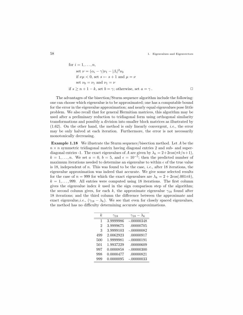
58 1. Eigenvalues and Eigenvectors
for i = 1, . . . , n,
set ν = (αi − γ)ν1 − |βi|2ν0
if νµ < 0, set s← s + 1 and µ = ν
set ν0 = ν1 and ν1 = ν
if s ≥ n + 1− k, set b = γ; otherwise, set a = γ . 2
The advantages of the bisection/Sturm sequence algorithm include the following:one can choose which eigenvalue is to be approximated; one has a computable boundfor the error in the eigenvalue approximation; and nearly equal eigenvalues pose littleproblem. We also recall that for general Hermitian matrices, this algorithm may beused after a preliminary reduction to tridiagonal form using orthogonal similaritytransformations and possibly a division into smaller block matrices as illustrated by(1.62). On the other hand, the method is only linearly convergent, i.e., the errormay be only halved at each iteration. Furthermore, the error is not necessarilymonotonically decreasing.
Example 1.18 We illustrate the Sturm sequence/bisection method. Let A be then× n symmetric tridiagonal matrix having diagonal entries 2 and sub- and super-diagonal entries -1. The exact eigenvalues of A are given by λk = 2+2cos(πk/n+1),k = 1, . . . , n. We set a = 0, b = 5, and ε = 10−5; then the predicted number ofmaximum iterations needed to determine an eigenvalue to within ε of the true valueis 18, independent of n. This was found to be the case, i.e., after 18 iterations, theeigenvalue approximation was indeed that accurate. We give some selected resultsfor the case of n = 999 for which the exact eigenvalues are λk = 2 + 2cos(.001πk),k = 1, . . . , 999. All entries were computed using 18 iterations. The first columngives the eigenvalue index k used in the sign comparison step of the algorithm;the second column gives, for each k, the approximate eigenvalue γ18 found after18 iterations; and the third column the difference between the approximate andexact eigenvalue,i.e., (γ18 − λk). We see that even for closely spaced eigenvalues,the method has no difficulty determining accurate approximations.
k γ18 γ18 − λk
1 3.9999986 -.000003482 3.9999675 .000007053 3.9999103 -.00000082
499 2.0062923 .00000917500 1.9999981 -.00000191501 1.9937229 .00000609997 0.0000858 -.00000300998 0.0000477 .00000821999 0.0000095 -.00000033
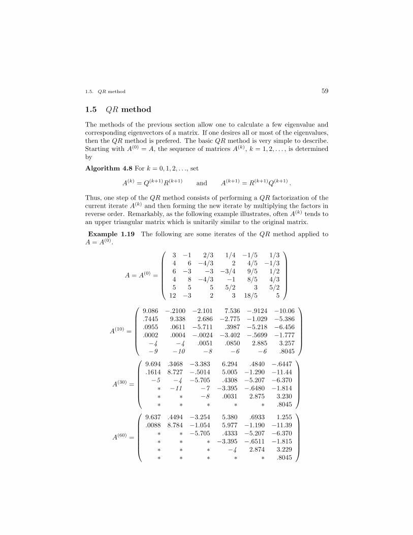
1.5. QR method 59
1.5 QR method
The methods of the previous section allow one to calculate a few eigenvalue andcorresponding eigenvectors of a matrix. If one desires all or most of the eigenvalues,then the QR method is prefered. The basic QR method is very simple to describe.Starting with A(0) = A, the sequence of matrices A(k), k = 1, 2, . . . , is determinedby
Algorithm 4.8 For k = 0, 1, 2, . . ., set
A(k) = Q(k+1)R(k+1) and A(k+1) = R(k+1)Q(k+1) .
Thus, one step of the QR method consists of performing a QR factorization of thecurrent iterate A(k) and then forming the new iterate by multiplying the factors inreverse order. Remarkably, as the following example illustrates, often A(k) tends toan upper triangular matrix which is unitarily similar to the original matrix.
Example 1.19 The following are some iterates of the QR method applied toA = A(0).
A = A(0) =
3 −1 2/3 1/4 −1/5 1/34 6 −4/3 2 4/5 −1/36 −3 −3 −3/4 9/5 1/24 8 −4/3 −1 8/5 4/35 5 5 5/2 3 5/2
12 −3 2 3 18/5 5
A(10) =
9.086 −.2100 −2.101 7.536 −.9124 −10.06.7445 9.338 2.686 −2.775 −1.029 −5.386.0955 .0611 −5.711 .3987 −5.218 −6.456.0002 .0004 −.0024 −3.402 −.5699 −1.777−4 −4 .0051 .0850 2.885 3.257−9 −10 −8 −6 −6 .8045
A(30) =
9.694 .3468 −3.383 6.294 .4840 −.6447.1614 8.727 −.5014 5.005 −1.290 −11.44−5 −4 −5.705 .4308 −5.207 −6.370∗ −11 −7 −3.395 −.6480 −1.814∗ ∗ −8 .0031 2.875 3.230∗ ∗ ∗ ∗ ∗ .8045
A(60) =
9.637 .4494 −3.254 5.380 .6933 1.255.0088 8.784 −1.054 5.977 −1.190 −11.39∗ ∗ −5.705 .4333 −5.207 −6.370∗ ∗ ∗ −3.395 −.6511 −1.815∗ ∗ ∗ −4 2.874 3.229∗ ∗ ∗ ∗ ∗ .8045
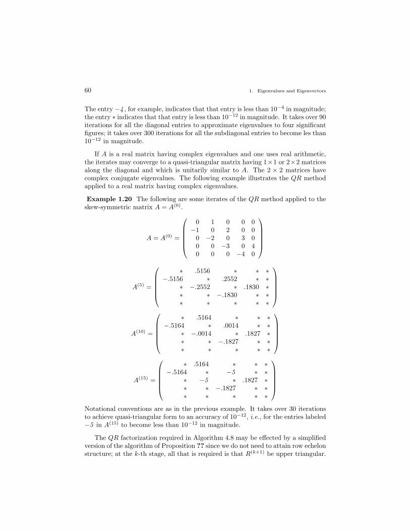
60 1. Eigenvalues and Eigenvectors
The entry −4 , for example, indicates that that entry is less than 10−4 in magnitude;the entry ∗ indicates that that entry is less than 10−12 in magnitude. It takes over 90iterations for all the diagonal entries to approximate eigenvalues to four significantfigures; it takes over 300 iterations for all the subdiagonal entries to become les than10−12 in magnitude.
If A is a real matrix having complex eigenvalues and one uses real arithmetic,the iterates may converge to a quasi-triangular matrix having 1×1 or 2×2 matricesalong the diagonal and which is unitarily similar to A. The 2 × 2 matrices havecomplex conjugate eigenvalues. The following example illustrates the QR methodapplied to a real matrix having complex eigenvalues.
Example 1.20 The following are some iterates of the QR method applied to theskew-symmetric matrix A = A(0).
A = A(0) =
0 1 0 0 0−1 0 2 0 0
0 −2 0 3 00 0 −3 0 40 0 0 −4 0
A(5) =
∗ .5156 ∗ ∗ ∗
−.5156 ∗ .2552 ∗ ∗∗ −.2552 ∗ .1830 ∗∗ ∗ −.1830 ∗ ∗∗ ∗ ∗ ∗ ∗
A(10) =
∗ .5164 ∗ ∗ ∗
−.5164 ∗ .0014 ∗ ∗∗ −.0014 ∗ .1827 ∗∗ ∗ −.1827 ∗ ∗∗ ∗ ∗ ∗ ∗
A(15) =
∗ .5164 ∗ ∗ ∗
−.5164 ∗ −5 ∗ ∗∗ −5 ∗ .1827 ∗∗ ∗ −.1827 ∗ ∗∗ ∗ ∗ ∗ ∗
Notational conventions are as in the previous example. It takes over 30 iterationsto achieve quasi-triangular form to an accuracy of 10−12, i.e., for the entries labeled−5 in A(15) to become less than 10−12 in magnitude.
The QR factorization required in Algorithm 4.8 may be effected by a simplifiedversion of the algorithm of Proposition ?? since we do not need to attain row echelonstructure; at the k-th stage, all that is required is that R(k+1) be upper triangular.
1.5. QR method 61
The QR method as defined by Algorithm 4.8 is impractical for two reasons.First, each step of the method requires a QR factorization which costs O(n3) mul-tiplications and a like number of additions or subtractions. Second, we have onlylinear convergence of the subdiagonal entries of A(k+1) to zero. Thus, the methodof Algorithm 4.8 requires too many steps and each step is too costly. Therefore, weexamine modifications to the basic method Algorithm 4.8 that transform it into apractical algortihm.
1.5.1 The practical QR method
The three essential ingredients in making the QR method practical are the use ofa preliminary reduction to upper Hessenberg form in order to reduce the cost periteration, the use of a deflation procedure whenever a subdiagonal entry effectivelyvanishes, again in order to reduce the cost per iteration, and the use of a shiftstrategy in order to accelerate convergence.
The Hessenberg QR iteration
In Section 1.3 it was shown that one may, in a finite number of arithmetic oper-ations, use unitary similarity transformations to reduce any square matrix to anupper Hessenberg matrix. In particular, we may use Algorithm 4.1 to find an upperHessenberg matrix A(0) that is unitarily similar to A. The following algorithm usesthis upper Hessenberg matrix as a starting point for the QR iteration.
Algorithm 4.9 Use Algorithm 1.1 to determine a matrix A(0) = Q(0)∗AQ(0) thatis upper Hessenberg and is unitarily similar to A.
For k = 0, 1, 2, . . ., set
A(k) = Q(k+1)R(k+1) and A(k+1) = R(k+1)Q(k+1) .
Another remarkable feature of the QR method is that it can always be arranged forall the iterates A(k), k = 1, 2, . . . , to be upper Hessenberg whenever A(0) is upperHessenberg. To see this, we first need to discuss how to use Givens rotations toefficiently determine the QR factorization of an upper Hessenberg matrix. Let Cbe an arbitrary n× n upper Hessenberg matrix.
Set R = C.
For j = 1, . . . , n− 1,
determine a 2× 2 Givens rotation G(j,j+1) such that
G(j,j+1)
(rj,j
rj+1,j
)=
( √r2j,j + r2
j+1,j
0
)
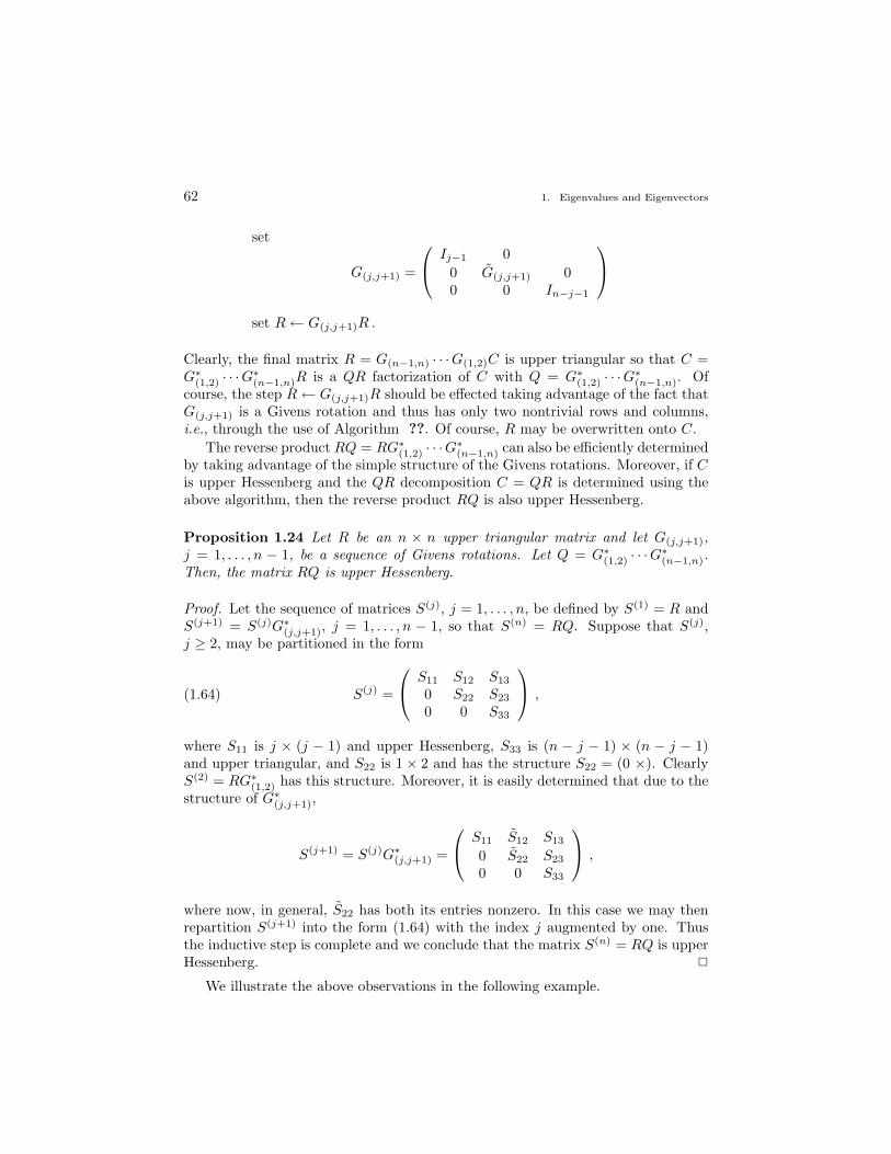
62 1. Eigenvalues and Eigenvectors
set
G(j,j+1) =
Ij−1 00 G(j,j+1) 00 0 In−j−1
set R← G(j,j+1)R .
Clearly, the final matrix R = G(n−1,n) · · ·G(1,2)C is upper triangular so that C =G∗(1,2) · · ·G
∗(n−1,n)R is a QR factorization of C with Q = G∗(1,2) · · ·G
∗(n−1,n). Of
course, the step R← G(j,j+1)R should be effected taking advantage of the fact thatG(j,j+1) is a Givens rotation and thus has only two nontrivial rows and columns,i.e., through the use of Algorithm ??. Of course, R may be overwritten onto C.
The reverse product RQ = RG∗(1,2) · · ·G∗(n−1,n) can also be efficiently determined
by taking advantage of the simple structure of the Givens rotations. Moreover, if Cis upper Hessenberg and the QR decomposition C = QR is determined using theabove algorithm, then the reverse product RQ is also upper Hessenberg.
Proposition 1.24 Let R be an n × n upper triangular matrix and let G(j,j+1),j = 1, . . . , n − 1, be a sequence of Givens rotations. Let Q = G∗(1,2) · · ·G
∗(n−1,n).
Then, the matrix RQ is upper Hessenberg.
Proof. Let the sequence of matrices S(j), j = 1, . . . , n, be defined by S(1) = R andS(j+1) = S(j)G∗(j,j+1), j = 1, . . . , n − 1, so that S(n) = RQ. Suppose that S(j),j ≥ 2, may be partitioned in the form
S(j) =
S11 S12 S13
0 S22 S23
0 0 S33
,(1.64)
where S11 is j × (j − 1) and upper Hessenberg, S33 is (n − j − 1) × (n − j − 1)and upper triangular, and S22 is 1× 2 and has the structure S22 = (0 ×). ClearlyS(2) = RG∗(1,2) has this structure. Moreover, it is easily determined that due to thestructure of G∗(j,j+1),
S(j+1) = S(j)G∗(j,j+1) =
S11 S12 S13
0 S22 S23
0 0 S33
,
where now, in general, S22 has both its entries nonzero. In this case we may thenrepartition S(j+1) into the form (1.64) with the index j augmented by one. Thusthe inductive step is complete and we conclude that the matrix S(n) = RQ is upperHessenberg. 2
We illustrate the above observations in the following example.
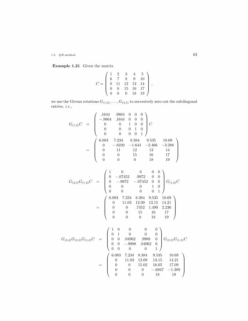
1.5. QR method 63
Example 1.21 Given the matrix
C =
1 2 3 4 56 7 8 9 100 11 12 13 140 0 15 16 170 0 0 18 19
,
we use the Givens rotations G(1,2), . . . , G(4,5) to succesively zero out the subdiagonalentries, i.e.,
G(1,2)C =
.1644 .9864 0 0 0−.9864 .1644 0 0 0
0 0 1 0 00 0 0 1 00 0 0 0 1
C
=
6.083 7.234 8.384 9.535 10.69
0 −.8220 −1.644 −2.466 −3.2880 11 12 13 140 0 15 16 170 0 0 18 19
G(2,3)G(1,2)C =
1 0 0 0 00 −.07452 .9972 0 00 −.9972 −.07452 0 00 0 0 1 00 0 0 0 1
G(1,2)C
=
6.083 7.234 8.384 9.535 10.69
0 11.03 12.09 13.15 14.210 0 .7452 1.490 2.2360 0 15 16 170 0 0 18 19
G(3,4)G(2,3)G(1,2)C =
1 0 0 0 00 1 0 0 00 0 .04962 .9988 00 0 −.9988 .04962 00 0 0 0 1
G(2,3)G(1,2)C
=
6.083 7.234 8.384 9.535 10.69
0 11.03 12.09 13.15 14.210 0 15.02 16.05 17.090 0 0 −.6947 −1.3890 0 0 18 19
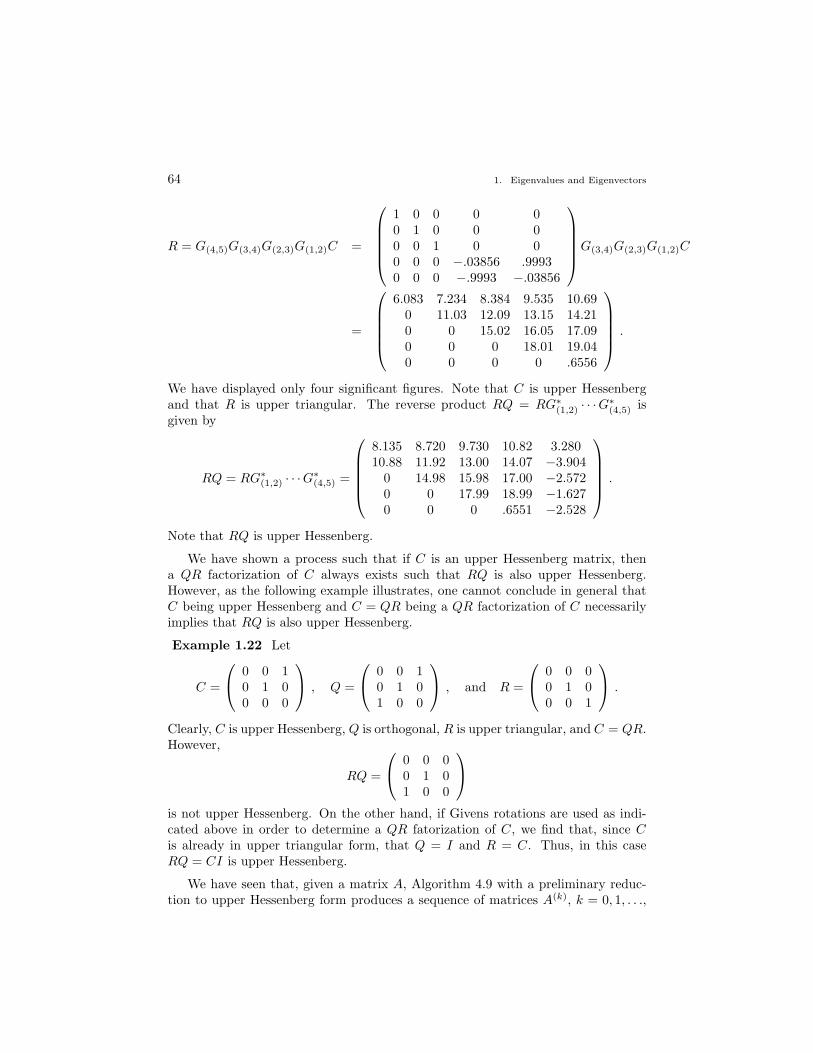
64 1. Eigenvalues and Eigenvectors
R = G(4,5)G(3,4)G(2,3)G(1,2)C =
1 0 0 0 00 1 0 0 00 0 1 0 00 0 0 −.03856 .99930 0 0 −.9993 −.03856
G(3,4)G(2,3)G(1,2)C
=
6.083 7.234 8.384 9.535 10.69
0 11.03 12.09 13.15 14.210 0 15.02 16.05 17.090 0 0 18.01 19.040 0 0 0 .6556
.
We have displayed only four significant figures. Note that C is upper Hessenbergand that R is upper triangular. The reverse product RQ = RG∗(1,2) · · ·G
∗(4,5) is
given by
RQ = RG∗(1,2) · · ·G∗(4,5) =
8.135 8.720 9.730 10.82 3.28010.88 11.92 13.00 14.07 −3.904
0 14.98 15.98 17.00 −2.5720 0 17.99 18.99 −1.6270 0 0 .6551 −2.528
.
Note that RQ is upper Hessenberg.
We have shown a process such that if C is an upper Hessenberg matrix, thena QR factorization of C always exists such that RQ is also upper Hessenberg.However, as the following example illustrates, one cannot conclude in general thatC being upper Hessenberg and C = QR being a QR factorization of C necessarilyimplies that RQ is also upper Hessenberg.
Example 1.22 Let
C =
0 0 10 1 00 0 0
, Q =
0 0 10 1 01 0 0
, and R =
0 0 00 1 00 0 1
.
Clearly, C is upper Hessenberg, Q is orthogonal, R is upper triangular, and C = QR.However,
RQ =
0 0 00 1 01 0 0
is not upper Hessenberg. On the other hand, if Givens rotations are used as indi-cated above in order to determine a QR fatorization of C, we find that, since Cis already in upper triangular form, that Q = I and R = C. Thus, in this caseRQ = CI is upper Hessenberg.
We have seen that, given a matrix A, Algorithm 4.9 with a preliminary reduc-tion to upper Hessenberg form produces a sequence of matrices A(k), k = 0, 1, . . .,
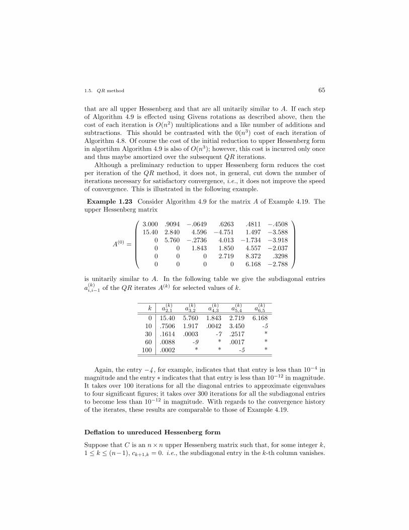
1.5. QR method 65
that are all upper Hessenberg and that are all unitarily similar to A. If each stepof Algorithm 4.9 is effected using Givens rotations as described above, then thecost of each iteration is O(n2) multiplications and a like number of additions andsubtractions. This should be contrasted with the 0(n3) cost of each iteration ofAlgorithm 4.8. Of course the cost of the initial reduction to upper Hessenberg formin algortihm Algorithm 4.9 is also of O(n3); however, this cost is incurred only onceand thus maybe amortized over the subsequent QR iterations.
Although a preliminary reduction to upper Hessenberg form reduces the costper iteration of the QR method, it does not, in general, cut down the number ofiterations necessary for satisfactory convergence, i.e., it does not improve the speedof convergence. This is illustrated in the following example.
Example 1.23 Consider Algorithm 4.9 for the matrix A of Example 4.19. Theupper Hessenberg matrix
A(0) =
3.000 .9094 −.0649 .6263 .4811 −.450815.40 2.840 4.596 −4.751 1.497 −3.588
0 5.760 −.2736 4.013 −1.734 −3.9180 0 1.843 1.850 4.557 −2.0370 0 0 2.719 8.372 .32980 0 0 0 6.168 −2.788
is unitarily similar to A. In the following table we give the subdiagonal entriesa(k)i,i−1 of the QR iterates A(k) for selected values of k.
k a(k)2,1 a
(k)3,2 a
(k)4,3 a
(k)5,4 a
(k)6,5
0 15.40 5.760 1.843 2.719 6.16810 .7506 1.917 .0042 3.450 -530 .1614 .0003 -7 .2517 *60 .0088 -9 * .0017 *
100 .0002 * * -5 *
Again, the entry −4 , for example, indicates that that entry is less than 10−4 inmagnitude and the entry ∗ indicates that that entry is less than 10−12 in magnitude.It takes over 100 iterations for all the diagonal entries to approximate eigenvaluesto four significant figures; it takes over 300 iterations for all the subdiagonal entriesto become less than 10−12 in magnitude. With regards to the convergence historyof the iterates, these results are comparable to those of Example 4.19.
Deflation to unreduced Hessenberg form
Suppose that C is an n×n upper Hessenberg matrix such that, for some integer k,1 ≤ k ≤ (n−1), ck+1,k = 0. i.e., the subdiagonal entry in the k-th column vanishes.
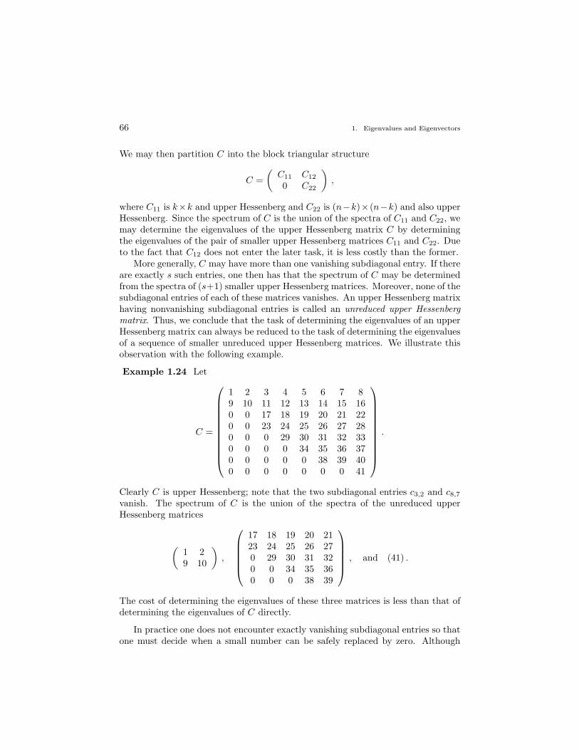
66 1. Eigenvalues and Eigenvectors
We may then partition C into the block triangular structure
C =(
C11 C12
0 C22
),
where C11 is k×k and upper Hessenberg and C22 is (n−k)× (n−k) and also upperHessenberg. Since the spectrum of C is the union of the spectra of C11 and C22, wemay determine the eigenvalues of the upper Hessenberg matrix C by determiningthe eigenvalues of the pair of smaller upper Hessenberg matrices C11 and C22. Dueto the fact that C12 does not enter the later task, it is less costly than the former.
More generally, C may have more than one vanishing subdiagonal entry. If thereare exactly s such entries, one then has that the spectrum of C may be determinedfrom the spectra of (s+1) smaller upper Hessenberg matrices. Moreover, none of thesubdiagonal entries of each of these matrices vanishes. An upper Hessenberg matrixhaving nonvanishing subdiagonal entries is called an unreduced upper Hessenbergmatrix. Thus, we conclude that the task of determining the eigenvalues of an upperHessenberg matrix can always be reduced to the task of determining the eigenvaluesof a sequence of smaller unreduced upper Hessenberg matrices. We illustrate thisobservation with the following example.
Example 1.24 Let
C =
1 2 3 4 5 6 7 89 10 11 12 13 14 15 160 0 17 18 19 20 21 220 0 23 24 25 26 27 280 0 0 29 30 31 32 330 0 0 0 34 35 36 370 0 0 0 0 38 39 400 0 0 0 0 0 0 41
.
Clearly C is upper Hessenberg; note that the two subdiagonal entries c3,2 and c8,7
vanish. The spectrum of C is the union of the spectra of the unreduced upperHessenberg matrices
(1 29 10
),
17 18 19 20 2123 24 25 26 270 29 30 31 320 0 34 35 360 0 0 38 39
, and (41) .
The cost of determining the eigenvalues of these three matrices is less than that ofdetermining the eigenvalues of C directly.
In practice one does not encounter exactly vanishing subdiagonal entries so thatone must decide when a small number can be safely replaced by zero. Although
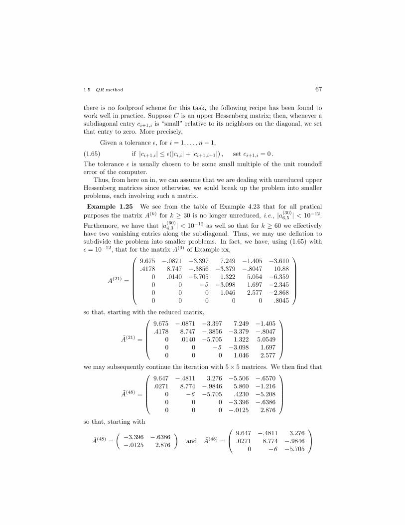
1.5. QR method 67
there is no foolproof scheme for this task, the following recipe has been found towork well in practice. Suppose C is an upper Hessenberg matrix; then, whenever asubdiagonal entry ci+1,i is “small” relative to its neighbors on the diagonal, we setthat entry to zero. More precisely,
Given a tolerance ε, for i = 1, . . . , n− 1,
if |ci+1,i| ≤ ε(|ci,i|+ |ci+1,i+1|) , set ci+1,i = 0 .(1.65)
The tolerance ε is usually chosen to be some small multiple of the unit roundofferror of the computer.
Thus, from here on in, we can assume that we are dealing with unreduced upperHessenberg matrices since otherwise, we sould break up the problem into smallerproblems, each involving such a matrix.
Example 1.25 We see from the table of Example 4.23 that for all praticalpurposes the matrix A(k) for k ≥ 30 is no longer unreduced, i.e., |a(30)
6,5 | < 10−12.
Furthemore, we have that |a(60)4,3 | < 10−12 as well so that for k ≥ 60 we effectively
have two vanishing entries along the subdiagonal. Thus, we may use deflation tosubdivide the problem into smaller problems. In fact, we have, using (1.65) withε = 10−12, that for the matrix A(0) of Example xx,
A(21) =
9.675 −.0871 −3.397 7.249 −1.405 −3.610.4178 8.747 −.3856 −3.379 −.8047 10.88
0 .0140 −5.705 1.322 5.054 −6.3590 0 −5 −3.098 1.697 −2.3450 0 0 1.046 2.577 −2.8680 0 0 0 0 .8045
so that, starting with the reduced matrix,
A(21) =
9.675 −.0871 −3.397 7.249 −1.405.4178 8.747 −.3856 −3.379 −.8047
0 .0140 −5.705 1.322 5.05490 0 −5 −3.098 1.6970 0 0 1.046 2.577
we may subsequently continue the iteration with 5× 5 matrices. We then find that
A(48) =
9.647 −.4811 3.276 −5.506 −.6570.0271 8.774 −.9846 5.860 −1.216
0 −6 −5.705 .4230 −5.2080 0 0 −3.396 −.63860 0 0 −.0125 2.876
so that, starting with
A(48) =(−3.396 −.6386−.0125 2.876
)and A(48) =
9.647 −.4811 3.276.0271 8.774 −.9846
0 −6 −5.705
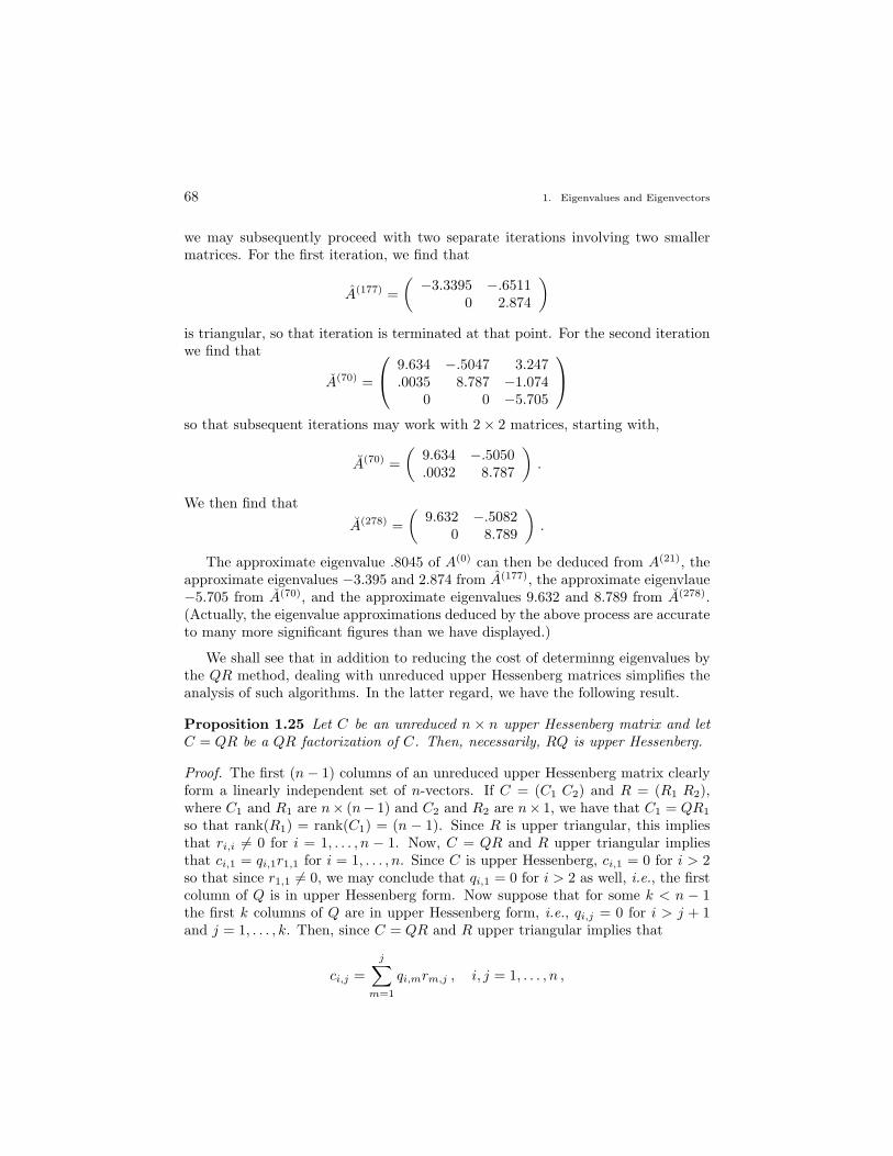
68 1. Eigenvalues and Eigenvectors
we may subsequently proceed with two separate iterations involving two smallermatrices. For the first iteration, we find that
A(177) =(−3.3395 −.6511
0 2.874
)is triangular, so that iteration is terminated at that point. For the second iterationwe find that
A(70) =
9.634 −.5047 3.247.0035 8.787 −1.074
0 0 −5.705
so that subsequent iterations may work with 2× 2 matrices, starting with,
A(70) =(
9.634 −.5050.0032 8.787
).
We then find that
A(278) =(
9.632 −.50820 8.789
).
The approximate eigenvalue .8045 of A(0) can then be deduced from A(21), theapproximate eigenvalues −3.395 and 2.874 from A(177), the approximate eigenvlaue−5.705 from A(70), and the approximate eigenvalues 9.632 and 8.789 from A(278).(Actually, the eigenvalue approximations deduced by the above process are accurateto many more significant figures than we have displayed.)
We shall see that in addition to reducing the cost of determinng eigenvalues bythe QR method, dealing with unreduced upper Hessenberg matrices simplifies theanalysis of such algorithms. In the latter regard, we have the following result.
Proposition 1.25 Let C be an unreduced n × n upper Hessenberg matrix and letC = QR be a QR factorization of C. Then, necessarily, RQ is upper Hessenberg.
Proof. The first (n− 1) columns of an unreduced upper Hessenberg matrix clearlyform a linearly independent set of n-vectors. If C = (C1 C2) and R = (R1 R2),where C1 and R1 are n× (n− 1) and C2 and R2 are n× 1, we have that C1 = QR1
so that rank(R1) = rank(C1) = (n − 1). Since R is upper triangular, this impliesthat ri,i 6= 0 for i = 1, . . . , n − 1. Now, C = QR and R upper triangular impliesthat ci,1 = qi,1r1,1 for i = 1, . . . , n. Since C is upper Hessenberg, ci,1 = 0 for i > 2so that since r1,1 6= 0, we may conclude that qi,1 = 0 for i > 2 as well, i.e., the firstcolumn of Q is in upper Hessenberg form. Now suppose that for some k < n − 1the first k columns of Q are in upper Hessenberg form, i.e., qi,j = 0 for i > j + 1and j = 1, . . . , k. Then, since C = QR and R upper triangular implies that
ci,j =j∑
m=1
qi,mrm,j , i, j = 1, . . . , n ,
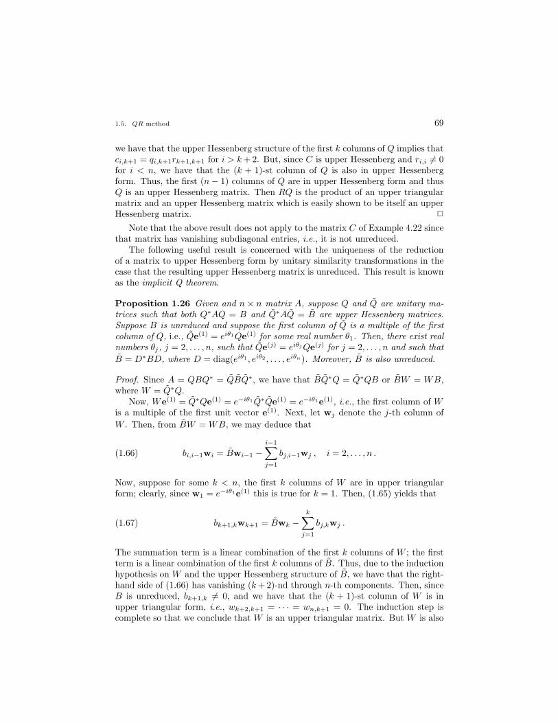
1.5. QR method 69
we have that the upper Hessenberg structure of the first k columns of Q implies thatci,k+1 = qi,k+1rk+1,k+1 for i > k + 2. But, since C is upper Hessenberg and ri,i 6= 0for i < n, we have that the (k + 1)-st column of Q is also in upper Hessenbergform. Thus, the first (n− 1) columns of Q are in upper Hessenberg form and thusQ is an upper Hessenberg matrix. Then RQ is the product of an upper triangularmatrix and an upper Hessenberg matrix which is easily shown to be itself an upperHessenberg matrix. 2
Note that the above result does not apply to the matrix C of Example 4.22 sincethat matrix has vanishing subdiagonal entries, i.e., it is not unreduced.
The following useful result is concerned with the uniqueness of the reductionof a matrix to upper Hessenberg form by unitary similarity transformations in thecase that the resulting upper Hessenberg matrix is unreduced. This result is knownas the implicit Q theorem.
Proposition 1.26 Given and n × n matrix A, suppose Q and Q are unitary ma-trices such that both Q∗AQ = B and Q∗AQ = B are upper Hessenberg matrices.Suppose B is unreduced and suppose the first column of Q is a multiple of the firstcolumn of Q, i.e., Qe(1) = eiθ1Qe(1) for some real number θ1. Then, there exist realnumbers θj, j = 2, . . . , n, such that Qe(j) = eiθj Qe(j) for j = 2, . . . , n and such thatB = D∗BD, where D = diag(eiθ1 , eiθ2 , . . . , eiθn). Moreover, B is also unreduced.
Proof. Since A = QBQ∗ = QBQ∗, we have that BQ∗Q = Q∗QB or BW = WB,where W = Q∗Q.
Now, We(1) = Q∗Qe(1) = e−iθ1Q∗Qe(1) = e−iθ1e(1), i.e., the first column of Wis a multiple of the first unit vector e(1). Next, let wj denote the j-th column ofW . Then, from BW = WB, we may deduce that
bi,i−1wi = Bwi−1 −i−1∑j=1
bj,i−1wj , i = 2, . . . , n .(1.66)
Now, suppose for some k < n, the first k columns of W are in upper triangularform; clearly, since w1 = e−iθ1e(1) this is true for k = 1. Then, (1.65) yields that
bk+1,kwk+1 = Bwk −k∑
j=1
bj,kwj .(1.67)
The summation term is a linear combination of the first k columns of W ; the firstterm is a linear combination of the first k columns of B. Thus, due to the inductionhypothesis on W and the upper Hessenberg structure of B, we have that the right-hand side of (1.66) has vanishing (k + 2)-nd through n-th components. Then, sinceB is unreduced, bk+1,k 6= 0, and we have that the (k + 1)-st column of W is inupper triangular form, i.e., wk+2,k+1 = · · · = wn,k+1 = 0. The induction step iscomplete so that we conclude that W is an upper triangular matrix. But W is also
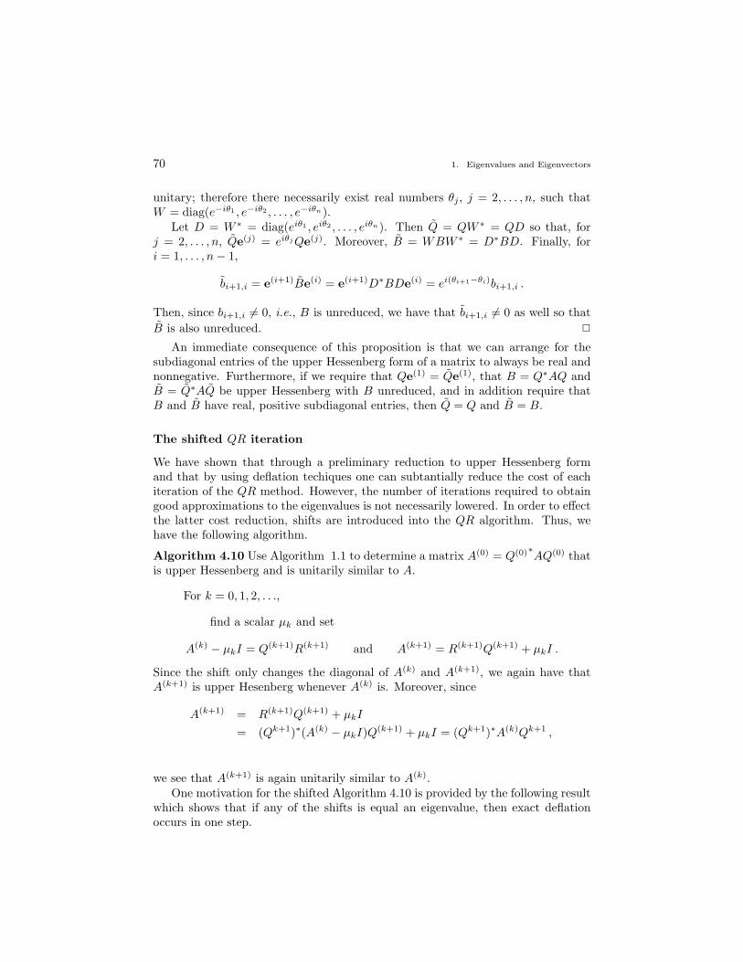
70 1. Eigenvalues and Eigenvectors
unitary; therefore there necessarily exist real numbers θj , j = 2, . . . , n, such thatW = diag(e−iθ1 , e−iθ2 , . . . , e−iθn).
Let D = W ∗ = diag(eiθ1 , eiθ2 , . . . , eiθn). Then Q = QW ∗ = QD so that, forj = 2, . . . , n, Qe(j) = eiθj Qe(j). Moreover, B = WBW ∗ = D∗BD. Finally, fori = 1, . . . , n− 1,
bi+1,i = e(i+1)Be(i) = e(i+1)D∗BDe(i) = ei(θi+1−θi)bi+1,i .
Then, since bi+1,i 6= 0, i.e., B is unreduced, we have that bi+1,i 6= 0 as well so thatB is also unreduced. 2
An immediate consequence of this proposition is that we can arrange for thesubdiagonal entries of the upper Hessenberg form of a matrix to always be real andnonnegative. Furthermore, if we require that Qe(1) = Qe(1), that B = Q∗AQ andB = Q∗AQ be upper Hessenberg with B unreduced, and in addition require thatB and B have real, positive subdiagonal entries, then Q = Q and B = B.
The shifted QR iteration
We have shown that through a preliminary reduction to upper Hessenberg formand that by using deflation techiques one can subtantially reduce the cost of eachiteration of the QR method. However, the number of iterations required to obtaingood approximations to the eigenvalues is not necessarily lowered. In order to effectthe latter cost reduction, shifts are introduced into the QR algorithm. Thus, wehave the following algorithm.
Algorithm 4.10 Use Algorithm 1.1 to determine a matrix A(0) = Q(0)∗AQ(0) thatis upper Hessenberg and is unitarily similar to A.
For k = 0, 1, 2, . . .,
find a scalar µk and set
A(k) − µkI = Q(k+1)R(k+1) and A(k+1) = R(k+1)Q(k+1) + µkI .
Since the shift only changes the diagonal of A(k) and A(k+1), we again have thatA(k+1) is upper Hesenberg whenever A(k) is. Moreover, since
A(k+1) = R(k+1)Q(k+1) + µkI
= (Qk+1)∗(A(k) − µkI)Q(k+1) + µkI = (Qk+1)∗A(k)Qk+1 ,
we see that A(k+1) is again unitarily similar to A(k).One motivation for the shifted Algorithm 4.10 is provided by the following result
which shows that if any of the shifts is equal an eigenvalue, then exact deflationoccurs in one step.
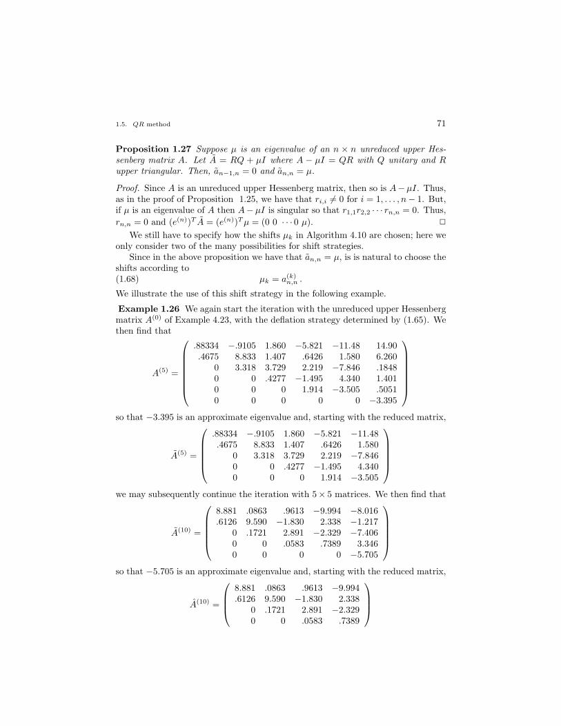
1.5. QR method 71
Proposition 1.27 Suppose µ is an eigenvalue of an n × n unreduced upper Hes-senberg matrix A. Let A = RQ + µI where A − µI = QR with Q unitary and Rupper triangular. Then, an−1,n = 0 and an,n = µ.
Proof. Since A is an unreduced upper Hessenberg matrix, then so is A−µI. Thus,as in the proof of Proposition 1.25, we have that ri,i 6= 0 for i = 1, . . . , n− 1. But,if µ is an eigenvalue of A then A− µI is singular so that r1,1r2,2 · · · rn,n = 0. Thus,rn,n = 0 and (e(n))T A = (e(n))T µ = (0 0 · · · 0 µ). 2
We still have to specify how the shifts µk in Algorithm 4.10 are chosen; here weonly consider two of the many possibilities for shift strategies.
Since in the above proposition we have that an,n = µ, is is natural to choose theshifts according to
µk = a(k)n,n .(1.68)
We illustrate the use of this shift strategy in the following example.
Example 1.26 We again start the iteration with the unreduced upper Hessenbergmatrix A(0) of Example 4.23, with the deflation strategy determined by (1.65). Wethen find that
A(5) =
.88334 −.9105 1.860 −5.821 −11.48 14.90.4675 8.833 1.407 .6426 1.580 6.260
0 3.318 3.729 2.219 −7.846 .18480 0 .4277 −1.495 4.340 1.4010 0 0 1.914 −3.505 .50510 0 0 0 0 −3.395
so that −3.395 is an approximate eigenvalue and, starting with the reduced matrix,
A(5) =
.88334 −.9105 1.860 −5.821 −11.48.4675 8.833 1.407 .6426 1.580
0 3.318 3.729 2.219 −7.8460 0 .4277 −1.495 4.3400 0 0 1.914 −3.505
we may subsequently continue the iteration with 5× 5 matrices. We then find that
A(10) =
8.881 .0863 .9613 −9.994 −8.016.6126 9.590 −1.830 2.338 −1.217
0 .1721 2.891 −2.329 −7.4060 0 .0583 .7389 3.3460 0 0 0 −5.705
so that −5.705 is an approximate eigenvalue and, starting with the reduced matrix,
A(10) =
8.881 .0863 .9613 −9.994.6126 9.590 −1.830 2.338
0 .1721 2.891 −2.3290 0 .0583 .7389
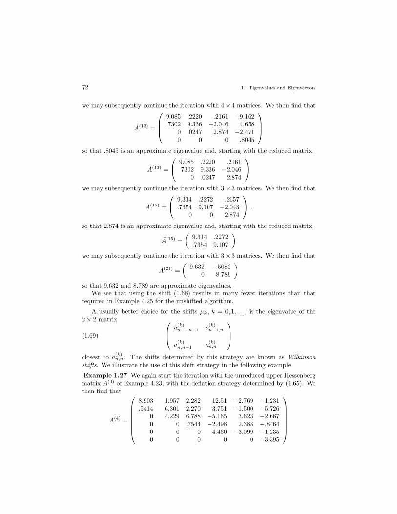
72 1. Eigenvalues and Eigenvectors
we may subsequently continue the iteration with 4× 4 matrices. We then find that
A(13) =
9.085 .2220 .2161 −9.162.7302 9.336 −2.046 4.658
0 .0247 2.874 −2.4710 0 0 .8045
so that .8045 is an approximate eigenvalue and, starting with the reduced matrix,
A(13) =
9.085 .2220 .2161.7302 9.336 −2.046
0 .0247 2.874
we may subsequently continue the iteration with 3× 3 matrices. We then find that
A(15) =
9.314 .2272 −.2657.7354 9.107 −2.043
0 0 2.874
.
so that 2.874 is an approximate eigenvalue and, starting with the reduced matrix,
A(15) =(
9.314 .2272.7354 9.107
)we may subsequently continue the iteration with 3× 3 matrices. We then find that
A(21) =(
9.632 −.50820 8.789
)so that 9.632 and 8.789 are approximate eigenvalues.
We see that using the shift (1.68) results in many fewer iterations than thatrequired in Example 4.25 for the unshifted algorithm.
A usually better choice for the shifts µk, k = 0, 1, . . ., is the eigenvalue of the2× 2 matrix a
(k)n−1,n−1 a
(k)n−1,n
a(k)n,n−1 a
(k)n,n
(1.69)
closest to a(k)n,n. The shifts determined by this strategy are known as Wilkinson
shifts. We illustrate the use of this shift strategy in the following example.
Example 1.27 We again start the iteration with the unreduced upper Hessenbergmatrix A(0) of Example 4.23, with the deflation strategy determined by (1.65). Wethen find that
A(4) =
8.903 −1.957 2.282 12.51 −2.769 −1.231.5414 6.301 2.270 3.751 −1.500 −5.726
0 4.229 6.788 −5.165 3.623 −2.6670 0 .7544 −2.498 2.388 −.84640 0 0 4.460 −3.099 −1.2350 0 0 0 0 −3.395
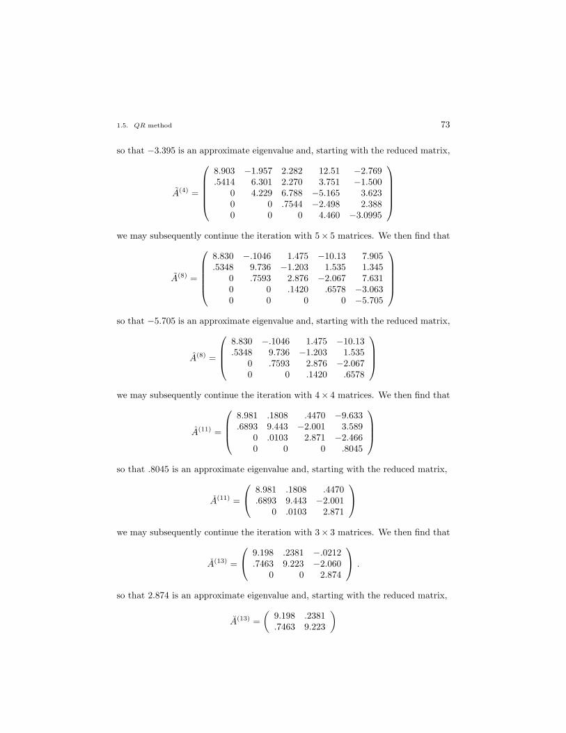
1.5. QR method 73
so that −3.395 is an approximate eigenvalue and, starting with the reduced matrix,
A(4) =
8.903 −1.957 2.282 12.51 −2.769.5414 6.301 2.270 3.751 −1.500
0 4.229 6.788 −5.165 3.6230 0 .7544 −2.498 2.3880 0 0 4.460 −3.0995
we may subsequently continue the iteration with 5× 5 matrices. We then find that
A(8) =
8.830 −.1046 1.475 −10.13 7.905.5348 9.736 −1.203 1.535 1.345
0 .7593 2.876 −2.067 7.6310 0 .1420 .6578 −3.0630 0 0 0 −5.705
so that −5.705 is an approximate eigenvalue and, starting with the reduced matrix,
A(8) =
8.830 −.1046 1.475 −10.13.5348 9.736 −1.203 1.535
0 .7593 2.876 −2.0670 0 .1420 .6578
we may subsequently continue the iteration with 4× 4 matrices. We then find that
A(11) =
8.981 .1808 .4470 −9.633.6893 9.443 −2.001 3.589
0 .0103 2.871 −2.4660 0 0 .8045
so that .8045 is an approximate eigenvalue and, starting with the reduced matrix,
A(11) =
8.981 .1808 .4470.6893 9.443 −2.001
0 .0103 2.871
we may subsequently continue the iteration with 3× 3 matrices. We then find that
A(13) =
9.198 .2381 −.0212.7463 9.223 −2.060
0 0 2.874
.
so that 2.874 is an approximate eigenvalue and, starting with the reduced matrix,
A(13) =(
9.198 .2381.7463 9.223
)
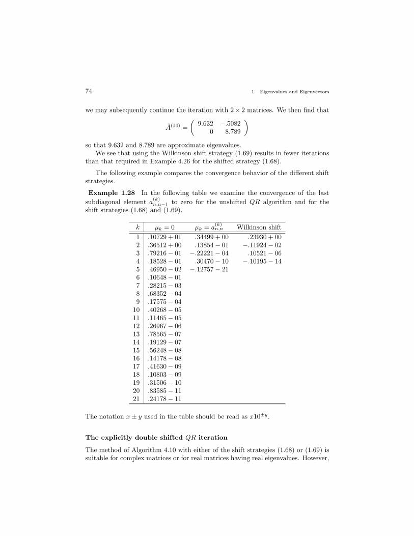
74 1. Eigenvalues and Eigenvectors
we may subsequently continue the iteration with 2× 2 matrices. We then find that
A(14) =(
9.632 −.50820 8.789
)so that 9.632 and 8.789 are approximate eigenvalues.
We see that using the Wilkinson shift strategy (1.69) results in fewer iterationsthan that required in Example 4.26 for the shifted strategy (1.68).
The following example compares the convergence behavior of the different shiftstrategies.
Example 1.28 In the following table we examine the convergence of the lastsubdiagonal element a
(k)n,n−1 to zero for the unshifted QR algorithm and for the
shift strategies (1.68) and (1.69).
k µk = 0 µk = a(k)n,n Wilkinson shift
1 .10729 + 01 .34499 + 00 .23930 + 002 .36512 + 00 .13854− 01 −.11924− 023 .79216− 01 −.22221− 04 .10521− 064 .18528− 01 .30470− 10 −.10195− 145 .46950− 02 −.12757− 216 .10648− 017 .28215− 038 .68352− 049 .17575− 04
10 .40268− 0511 .11465− 0512 .26967− 0613 .78565− 0714 .19129− 0715 .56248− 0816 .14178− 0817 .41630− 0918 .10803− 0919 .31506− 1020 .83585− 1121 .24178− 11
The notation x± y used in the table should be read as x10±y.
The explicitly double shifted QR iteration
The method of Algorithm 4.10 with either of the shift strategies (1.68) or (1.69) issuitable for complex matrices or for real matrices having real eigenvalues. However,
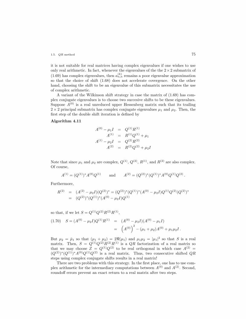
1.5. QR method 75
it is not suitable for real matrices having complex eigenvalues if one wishes to useonly real arithmetic. In fact, whenever the eigenvalues of the the 2×2 submatrix of(1.69) has complex eigenvalues, then a
(k)n,n remains a poor eigenvalue approximation
so that the choice of shift (1.68) does not accelerate covergence. On the otherhand, choosing the shift to be an eigenvalue of this submatrix necessitates the useof complex arithmetic.
A variant of the Wilkinson shift strategy in case the matrix of (1.69) has com-plex conjugate eigenvalues is to choose two succesive shifts to be these eigenvalues.Suppose A(0) is a real unreduced upper Hessenberg matrix such that its trailing2× 2 principal submatrix has complex conjugate eigenvalues µ1 and µ2. Then, thefirst step of the double shift iteration is defined by
Algorithm 4.11
A(0) − µ1I = Q(1)R(1)
A(1) = R(1)Q(1) + µ1
A(1) − µ2I = Q(2)R(2)
A(2) = R(2)Q(2) + µ2I
Note that since µ1 and µ2 are complex, Q(1), Q(2), R(1), and R(2) are also complex.Of course,
A(1) = (Q(1))∗A(0)Q(1) and A(2) = (Q(2))∗(Q(1))∗A(0)Q(1)Q(2) .
Furthermore,
R(2) = (A(2) − µ2I)(Q(2))∗ = (Q(2))∗(Q(1))∗(A(0) − µ2I)Q(1)Q(2)(Q(2))∗
= (Q(2))∗(Q(1))∗(A(0) − µ2I)Q(1)
so that, if we let S = Q(1)Q(2)R(2)R(1),
S = (A(0) − µ2I)Q(1)R(1) = (A(0) − µ2I)(A(0) − µ1I)(1.70)
=(A(0)
)2
− (µ1 + µ2)A(0) + µ1µ2I .
But µ2 = µ1 so that (µ1 + µ2) = 2<(µ1) and µ1µ2 = |µ1|2 so that S is a realmatrix. Then, S = Q(1)Q(2)R(2)R(1) is a QR factorization of a real matrix sothat we may choose Z = Q(1)Q(2) to be real orthogonal in which case A(2) =(Q(2))∗(Q(1))∗A(0)Q(1)Q(2) is a real matrix. Thus, two consecutive shifted QRsteps using complex conjugate shifts results in a real matrix!
There are two problems with this strategy. In the first place, one has to use com-plex arithmetic for the intermediary computations between A(0) and A(2). Second,roundoff errors prevent an exact return to a real matrix after two steps.
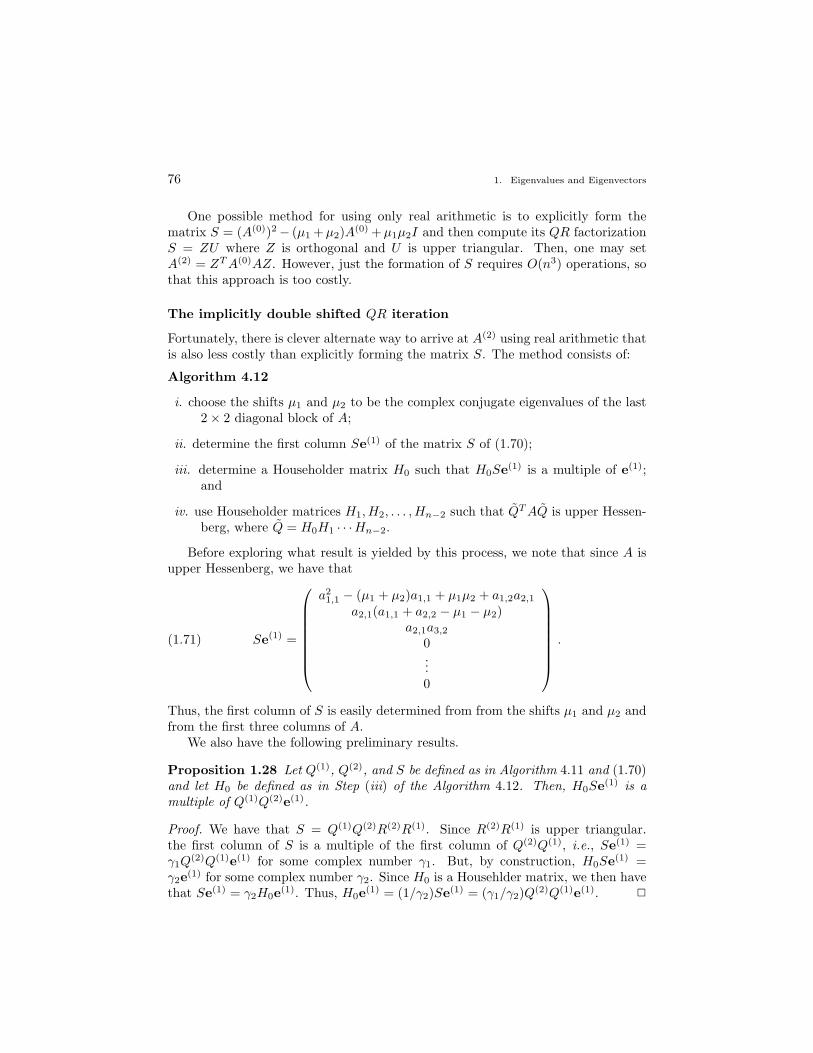
76 1. Eigenvalues and Eigenvectors
One possible method for using only real arithmetic is to explicitly form thematrix S = (A(0))2− (µ1 +µ2)A(0) +µ1µ2I and then compute its QR factorizationS = ZU where Z is orthogonal and U is upper triangular. Then, one may setA(2) = ZT A(0)AZ. However, just the formation of S requires O(n3) operations, sothat this approach is too costly.
The implicitly double shifted QR iteration
Fortunately, there is clever alternate way to arrive at A(2) using real arithmetic thatis also less costly than explicitly forming the matrix S. The method consists of:
Algorithm 4.12
i. choose the shifts µ1 and µ2 to be the complex conjugate eigenvalues of the last2× 2 diagonal block of A;
ii. determine the first column Se(1) of the matrix S of (1.70);
iii. determine a Householder matrix H0 such that H0Se(1) is a multiple of e(1);and
iv. use Householder matrices H1,H2, . . . ,Hn−2 such that QT AQ is upper Hessen-berg, where Q = H0H1 · · ·Hn−2.
Before exploring what result is yielded by this process, we note that since A isupper Hessenberg, we have that
Se(1) =
a21,1 − (µ1 + µ2)a1,1 + µ1µ2 + a1,2a2,1
a2,1(a1,1 + a2,2 − µ1 − µ2)a2,1a3,2
0...0
.(1.71)
Thus, the first column of S is easily determined from from the shifts µ1 and µ2 andfrom the first three columns of A.
We also have the following preliminary results.
Proposition 1.28 Let Q(1), Q(2), and S be defined as in Algorithm 4.11 and (1.70)and let H0 be defined as in Step (iii) of the Algorithm 4.12. Then, H0Se(1) is amultiple of Q(1)Q(2)e(1).
Proof. We have that S = Q(1)Q(2)R(2)R(1). Since R(2)R(1) is upper triangular.the first column of S is a multiple of the first column of Q(2)Q(1), i.e., Se(1) =γ1Q
(2)Q(1)e(1) for some complex number γ1. But, by construction, H0Se(1) =γ2e(1) for some complex number γ2. Since H0 is a Househlder matrix, we then havethat Se(1) = γ2H0e(1). Thus, H0e(1) = (1/γ2)Se(1) = (γ1/γ2)Q(2)Q(1)e(1). 2
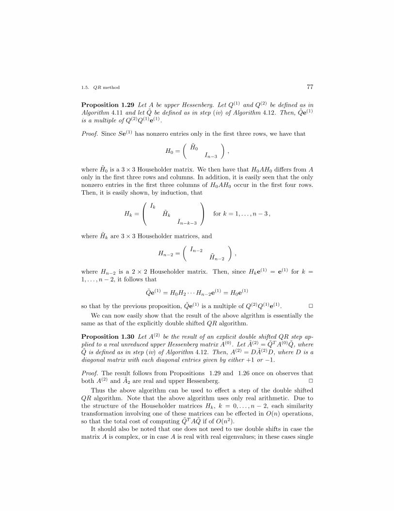
1.5. QR method 77
Proposition 1.29 Let A be upper Hessenberg. Let Q(1) and Q(2) be defined as inAlgorithm 4.11 and let Q be defined as in step (iv) of Algorithm 4.12. Then, Qe(1)
is a multiple of Q(2)Q(1)e(1).
Proof. Since Se(1) has nonzero entries only in the first three rows, we have that
H0 =(
H0
In−3
),
where H0 is a 3× 3 Householder matrix. We then have that H0AH0 differs from Aonly in the first three rows and columns. In addition, it is easily seen that the onlynonzero entries in the first three columns of H0AH0 occur in the first four rows.Then, it is easily shown, by induction, that
Hk =
Ik
Hk
In−k−3
for k = 1, . . . , n− 3 ,
where Hk are 3× 3 Householder matrices, and
Hn−2 =(
In−2
Hn−2
),
where Hn−2 is a 2 × 2 Householder matrix. Then, since Hke(1) = e(1) for k =1, . . . , n− 2, it follows that
Qe(1) = H0H2 · · ·Hn−2e(1) = H0e(1)
so that by the previous proposition, Qe(1) is a multiple of Q(2)Q(1)e(1). 2
We can now easily show that the result of the above algrithm is essentially thesame as that of the explicitly double shifted QR algorithm.
Proposition 1.30 Let A(2) be the result of an explicit double shifted QR step ap-plied to a real unreduced upper Hessenberg matrix A(0). Let A(2) = QT A(0)Q, whereQ is defined as in step (iv) of Algorithm 4.12. Then, A(2) = DA(2)D, where D is adiagonal matrix with each diagonal entries given by either +1 or −1.
Proof. The result follows from Propositions 1.29 and 1.26 once on observes thatboth A(2) and A2 are real and upper Hessenberg. 2
Thus the above algorithm can be used to effect a step of the double shiftedQR algorithm. Note that the above algorithm uses only real arithmetic. Due tothe structure of the Householder matrices Hk, k = 0, . . . , n − 2, each similaritytransformation involving one of these matrices can be effected in O(n) operations,so that the total cost of computing QT AQ if of O(n2).
It should also be noted that one does not need to use double shifts in case thematrix A is complex, or in case A is real with real eigenvalues; in these cases single
78 1. Eigenvalues and Eigenvectors
shifts will do. Furthermore, the double shifted QR algorithm does not converge forall matrices. For example, a double shifted QR step leaves the matrix
0 0 0 0 11 0 0 0 00 1 0 0 00 0 1 0 00 0 0 1 0
unchanged. Such hang-ups may be avoided by first applying two single shifted stepsbefore applying the double shifted stategy.
The practical QR algorithm
We now incorporate the various aspects of the practical implementation of the QRmethod into the following algorithm.
Algortihm 4.13
Given an n×n matrix A and a tolerance ε (usually ε > 0 is chosen to be somesmall multiple of the machine precision):
Use Householder transformations P0, P1, . . . , Pn−2 to determine a matrixB = Q∗AQ, Q = P0 · · ·Pn−2, that is upper Hessenberg and unitarilysimilar to A;
Do while q < n
if |bi,i−1| ≤ ε(|bi,i|+ |bi−1,i−1|), i = 2, . . . , n, set bi,i−1 = 0 ;
find the largest integer q ≥ 0 and smallest integer p ≥ 0 such that
B =
B11 B12 B13
0 B22 B23
0 0 B33
,
where B11 is p × p , B33 is q × q and quasi-triangular, and B22 isunreduced upper Hessenberg (note that p or q may vanish);
apply the implicit double shifted QR step to the (n−p−q)×(n−p−q)matrix B22 (set B22 ← QT BQ);
Compute the eigenvalues of the 2× 2 diagonal blocks of B.
Experience shows that, on the average, approximately two double shifted QRsteps are needed per decoupling, i.e., until a zero is detected somewhere along thesubdiagonal. In this case, all the eigenvalues may be located in approximately 10n3
operations.
1.5. QR method 79
1.5.2 The QR method for Hermitian matrices
We briefly consider the QR method for Hermitian matrices. First, we note that forsuch matrices, the preliminary reduction to upper Hessenberg form actually yieldsa Hermitian tridiagonal matrix. Next, we use the single shifted algorithm
A(k) − µkI = Q(k+1)R(k+1) and A(k+1) = R(k+1)Q(k+1) + µkI ,
where A(0) is a Hermitian tridiagonal matrix that is unitarily similar to the givenmatrix A. Since A(k+1) = (Q(k+1))∗A(k)Q(k+1), we have that A(k+1) is Hermitianwhenever A(k) is. Moerover, since a triadiagonal matrix is an upper Hessenbergmatrix, we have that A(k+1) is also upper Hessenberg. Thus, A(k+1) is tridiagonal,i.e., the shifted QR step preserves the Hermitian tridiagonal structure of a matrix.One may take advantage of this fact to implement each step of the QR iterationfor Hermiatian matrices in O(n) operations, as opposed to the O(n2) operationsrequired for general matrices.
Either of the shift startegies (1.68) or (1.69) may be used, although the Wilkinsonshift strategy (1.69) results in faster convergence. Note that since throughout theiteration one only deals with Hermitian matrices, that the shifts obtained fromeither (1.68) or (1.69) are always real so that for real symmetric matrices one doesnot need to employ the double shift strategy in order to work in real arithmetic.
As a result, for real symmetric matrices, we have the following practical QRalgortihm.
Algortihm 4.14
Given an n× n real symmetric matrix A and a tolerance ε:
Use real Householder transformations P0, P1, . . . , Pn−2 to determine amatrix B = Q∗AQ, Q = P0 · · ·Pn−2, that is symmetric, tridiagonal, andunitarily similar to A;Do while q < n
if |bi,i−1| ≤ ε(|bi,i|+ |bi−1,i−1|), i = 2, . . . , n, set bi,i−1 = 0 ;
find the largest integer q ≥ 0 and smallest integer p ≥ 0 such that
B =
B11 B12 B13
0 B22 B23
0 0 B33
,
where B11 is p× p , B33 is q× q and diagonal, and B22 is unreducedsymmetric tridiagonal (note that p or q may vanish);
apply the single shifted QR step with Wilkinson shifts to the (n −p− q)× (n− p− q) matrix B22.
Once again we note that this algorithm may be implemented in real arithmetic.Also, one may define an implicit single shift strategy so that the matrix A(k) − µkIneed not be explicitly formed.
80 1. Eigenvalues and Eigenvectors
1.5.3 The convergence of the QR
There are two types of convergence results avialable for the QR method. (Here, weonly consider the general single shifted version of the method for general complexmatrices.) The first type examines the whole subdiagonal triangle of the iteratesand shows that all the entries of that triangle tend to zero, i.e., the iterates convergeto an upper triangular matrix. The second looks at a particular row or column ofthe subdiagonal triangle and shows that the entries of that section of the matrixconverge to zero. Since once this happens one can deflate to a smaller matrix, thesecond view also shows that the QR method converges to a triangular matrix.
From a practical point viewpoint as well, both types of convergence results areimportant. The second view may be used to show why one is able to deflate, andalso how some particular subdiagonal elements converge to zero very quickly. Theseare crucial to the understanding of the practical QR method. The first view is alsoimportant because it shows that all of the subdiagonal entries are reduced duringthe QR iteration, and although not all reduce very quickly, the fact that they doreduce also helps explain the rapid convergence of the overall method.
Here, we will only consider the second viewpoint. We begin by considering theconeection between the shifted QR method and the shifted power and inverse powermethods.
Given an n × n matrix A and a sequence of shifts µk, k = 0, 1, . . . , cosider thefollowing three sequences. First, we have sequence of matrices obtained from theshifted QR method:
A(k+1) = (Q(k+1))∗A(k)Q(k+1) and A(k) − µkI = Q(k+1)R(k+1) ,(1.72)
where A(0) = A. The second is the shifted power method iteration for the matrixA with shifts given by µk:
p(k+1) =1αk
(A− µkI)p(k) , ‖p(k+1)‖2 = 1 ,(1.73)
where p(0) is any unit vector. The scale factors αk are determined by the require-ment that ‖p(k+1)‖2 = 1. The third is the shifted power method iteration for thematrix A∗ with shifts given by µk:
(A∗ − µkI)u(k+1) = βku(k) , ‖u(k+1)‖2 = 1 ,(1.74)
where u(0) is any unit vector. Again, the scale factors βk are determined by therequirement that ‖u(k+1)‖2 = 1.
The relation between these three iterations is given in the following result whichmakes use of the matrices
V (0) = I and V (k) = Q(1) · · ·Q(k) , k = 1, 2, . . . .(1.75)
Note that for k ≥ 0,
A(k+1) = (Q(k+1))∗A(k)Q(k+1) = (V (k+1))∗AV (k+1) .(1.76)
1.5. QR method 81
Proposition 1.31 Let the matrices A(k) and unit vectors p(k) and u(k), k =0, 1, . . . , be defined by (1.72), (1.73), and (1.74), respectively. Let none of the shiftsµk be an eigenvalue of A. Let p(0) = e(1) and u(0) = e(n). Then, for k = 1, 2, . . . ,
p(k) = V (k)e(1) and u(k) = V (k)e(n) .(1.77)
Proof. From (1.76) we have that
V (k)A(k) = AV (k)
so that, from (1.72) and (1.75),
V (k+1)R(k+1) = V (k)Q(k+1)R(k+1) = V (k)(A(k) − µkI) = (A− µkI)V (k) .(1.78)
Equating the first columns we have that
V (k+1)R(k+1)e(1) = (A− µkI)V (k)e(1)
and then, since R(k+1) is upper triangular,
V (k+1)e(1) =1
r(k+1)1,1
(A− µkI)V (k)e(1) .
Since ‖V (k+1)e(1)‖2 = 1, comparison with (1.73) yields the first of (1.77).Now, from (1.78), we have that
(R(k+1))∗(V (k+1))∗ = (V (k))∗(A∗ − µkI)
so thatV (k)(R(k+1))∗ = (A∗ − µkI)V (k+1) .
Then, since (R(k+1))∗ is lower triangular,
V (k)(R(k+1))∗e(n) = r(k+1)n,n V (k)e(n) = (A∗ − µkI)V (k+1)e(n) .
Since ‖V (k+1)e(n)‖2 = 1, comparison with (1.74) yields the second of (1.77). 2
The convergence proof we give applies to the basic, unshifted QR method.
Theorem 1.32 Let A be an n×n nondefective matrix. Let (λj ,q(j)), j = 1, . . . , n,denote the eigenpairs of A. Assume that
0 < |λ1| < |λ2| ≤ |λ3| ≤ · · · ≤ |λn−1| < |λn|
and that ‖q(1)‖2 = ‖q(n)‖2 = 1. Assume that for j = 1 and n, (e(j))∗q(j) 6= 0.Then, as k →∞,
A(k)e(1) → λne(1) and (e(n))T A(k) → λ1(e(n))T .
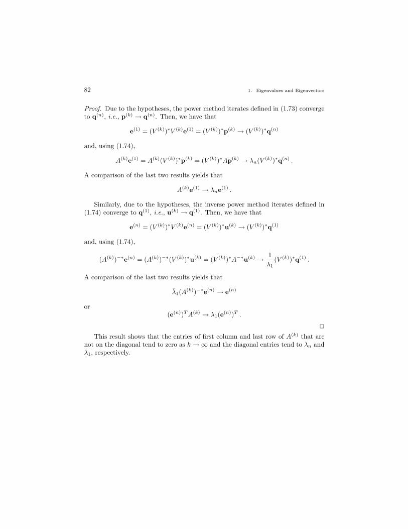
82 1. Eigenvalues and Eigenvectors
Proof. Due to the hypotheses, the power method iterates defined in (1.73) convergeto q(n), i.e., p(k) → q(n). Then, we have that
e(1) = (V (k))∗V (k)e(1) = (V (k))∗p(k) → (V (k))∗q(n)
and, using (1.74),
A(k)e(1) = A(k)(V (k))∗p(k) = (V (k))∗Ap(k) → λn(V (k))∗q(n) .
A comparison of the last two results yields that
A(k)e(1) → λne(1) .
Similarly, due to the hypotheses, the inverse power method iterates defined in(1.74) converge to q(1), i.e., u(k) → q(1). Then, we have that
e(n) = (V (k))∗V (k)e(n) = (V (k))∗u(k) → (V (k))∗q(1)
and, using (1.74),
(A(k))−∗e(n) = (A(k))−∗(V (k))∗u(k) = (V (k))∗A−∗u(k) → 1λ1
(V (k))∗q(1) .
A comparison of the last two results yields that
λ1(A(k))−∗e(n) → e(n)
or(e(n))T A(k) → λ1(e(n))T .
2
This result shows that the entries of first column and last row of A(k) that arenot on the diagonal tend to zero as k →∞ and the diagonal entries tend to λn andλ1, respectively.


![EIGENVECTORS, EIGENVALUES, AND FINITE STRAIN · unit vector, λ is the length of ... E Eigenvectors have corresponding eigenvalues, and vice-versa F In Matlab, [v,d] = eig(A), ...](https://static.fdocument.org/doc/165x107/5b32041f7f8b9aed688bb633/eigenvectors-eigenvalues-and-finite-strain-unit-vector-is-the-length-of.jpg)