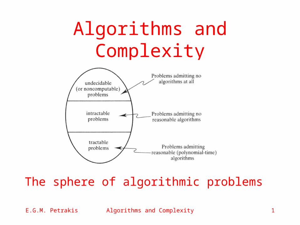
E.G.M. PetrakisAlgorithms and Complexity1 The sphere of algorithmic problems.
41
E.G.M. Petrakis Algorithms and Complexity 1 Algorithms and Complexity The sphere of algorithmic problems
-
date post
20-Dec-2015 -
Category
Documents
-
view
221 -
download
0
Transcript of E.G.M. PetrakisAlgorithms and Complexity1 The sphere of algorithmic problems.
E.G.M. Petrakis Algorithms and Complexity 1
Algorithms and Complexity
The sphere of algorithmic problems
E.G.M. Petrakis Algorithms and Complexity 2
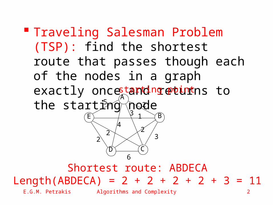
Traveling Salesman Problem (TSP): find the shortest route that passes though each of the nodes in a graph exactly once and returns to the starting node
Α
Ε
D
B
C
25
322 2
4
3 1
6
Shortest route: ABDECALength(ABDECA) = 2 + 2 + 2 + 2 + 3 = 11
starting point
E.G.M. Petrakis Algorithms and Complexity 3
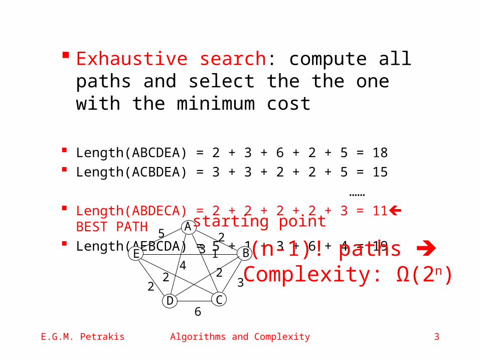
Exhaustive search: compute all paths and select the the one with the minimum cost
Length(ABCDEA) = 2 + 3 + 6 + 2 + 5 = 18 Length(ACBDEA) = 3 + 3 + 2 + 2 + 5 = 15 …… Length(ABDECA) = 2 + 2 + 2 + 2 + 3 = 11 BEST
PATH Length(AEBCDA) = 5 + 1 + 3 + 6 + 4 = 19
Α
Ε
D
B
C
25
322 2
43 1
6
(n-1)! paths Complexity: Ω(2n)
starting point
E.G.M. Petrakis Algorithms and Complexity 4
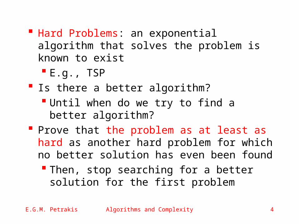
Hard Problems: an exponential algorithm that solves the problem is known to exist E.g., TSP
Is there a better algorithm? Until when do we try to find a better
algorithm? Prove that the problem as at least as
hard as another hard problem for which no better solution has even been found Then, stop searching for a better
solution for the first problem
E.G.M. Petrakis Algorithms and Complexity 5
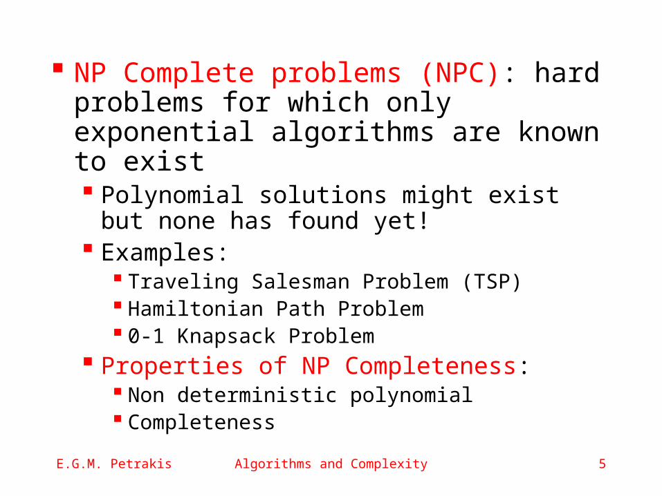
NP Complete problems (NPC): hard problems for which only exponential algorithms are known to exist Polynomial solutions might exist but
none has found yet! Examples:
Traveling Salesman Problem (TSP) Hamiltonian Path Problem 0-1 Knapsack Problem
Properties of NP Completeness: Non deterministic polynomial Completeness
E.G.M. Petrakis Algorithms and Complexity 6
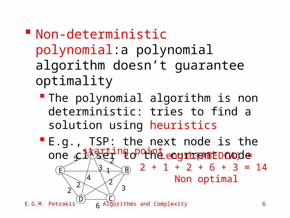
Non-deterministic polynomial:a polynomial algorithm doesn’t guarantee optimality The polynomial algorithm is non
deterministic: tries to find a solution using heuristics
E.g., TSP: the next node is the one closer to the current node
Α
Ε
D
B
C
25
322 2
43 1
6
Length(ABEDCA) =2 + 1 + 2 + 6 + 3 = 14
Non optimal
starting point
E.G.M. Petrakis Algorithms and Complexity 7
Completeness: if an optimal algorithm exists for one of the them, then a polynomial algorithm can be found for all It is possible to transform each problem
to another using a polynomial algorithm The complexity for solving a different
problem is the complexity of transforming the problem to the original one (takes polynomial time) plus the complexity of solving the original problem (take polynomial time again)!
E.G.M. Petrakis Algorithms and Complexity 8
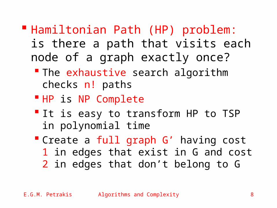
Hamiltonian Path (HP) problem: is there a path that visits each node of a graph exactly once? The exhaustive search algorithm
checks n! paths HP is NP Complete It is easy to transform HP to TSP in
polynomial time Create a full graph G’ having cost 1 in
edges that exist in G and cost 2 in edges that don’t belong to G
E.G.M. Petrakis Algorithms and Complexity 9
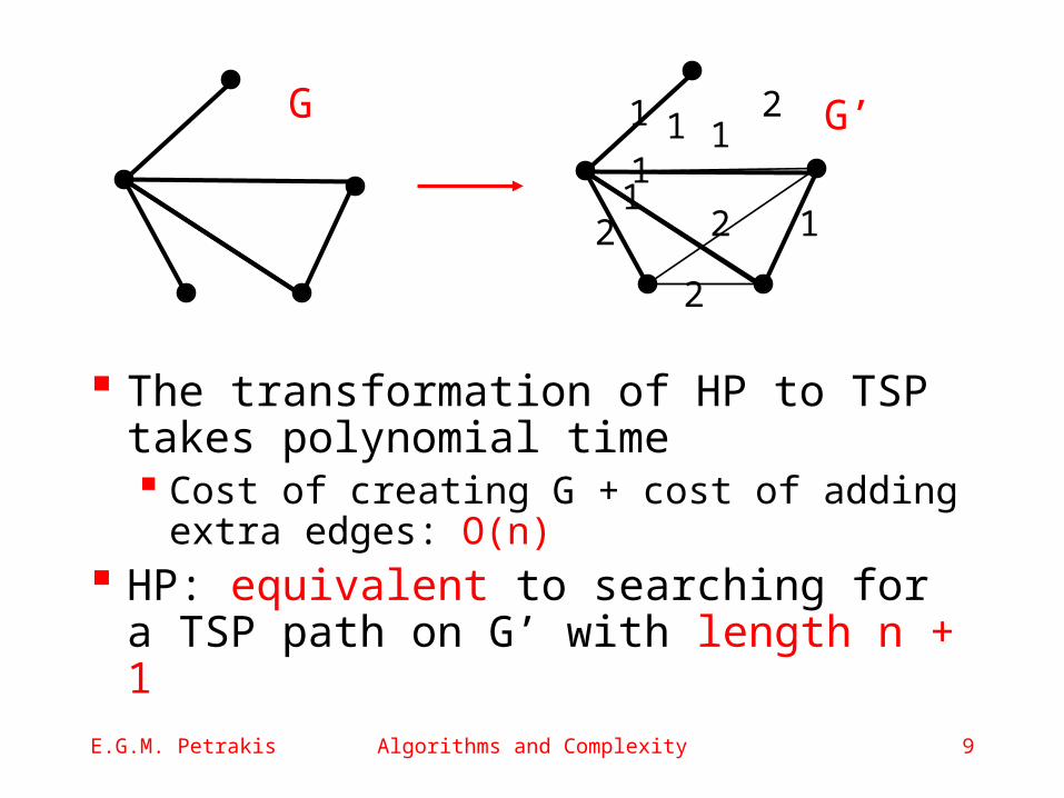
The transformation of HP to TSP takes polynomial time Cost of creating G + cost of adding
extra edges: O(n) HP: equivalent to searching for a
TSP path on G’ with length n + 1
1
11
1 1
1
2
2
2
2
G G’
E.G.M. Petrakis Algorithms and Complexity 10
Algorithms
Types of Heuristic algorithms Greedy Local search
Types of Optimal algorithms Exhaustive Search (ES) Divide and Conquer (D&C) Branch and Bound (B&B) Dynamic Programming (DP)
E.G.M. Petrakis Algorithms and Complexity 11
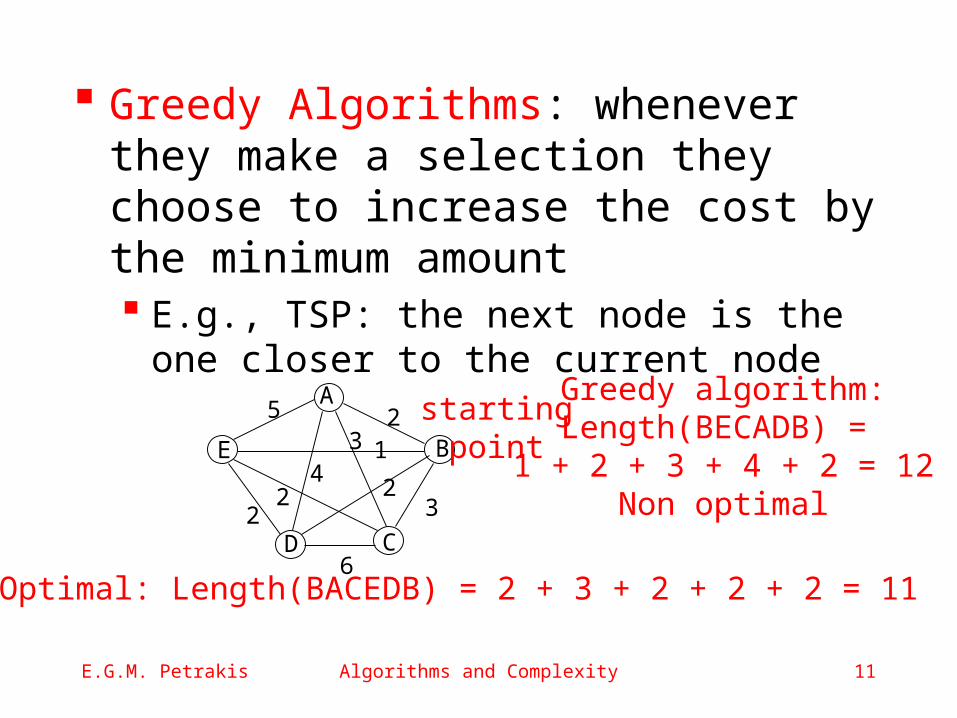
Greedy Algorithms: whenever they make a selection they choose to increase the cost by the minimum amount E.g., TSP: the next node is the one
closer to the current nodeΑ
Ε
D
B
C
25
322 2
43 1
6
startingpoint
Greedy algorithm:Length(BECADB) = 1 + 2 + 3 + 4 + 2 = 12
Non optimal
Optimal: Length(BACEDB) = 2 + 3 + 2 + 2 + 2 = 11
E.G.M. Petrakis Algorithms and Complexity 12
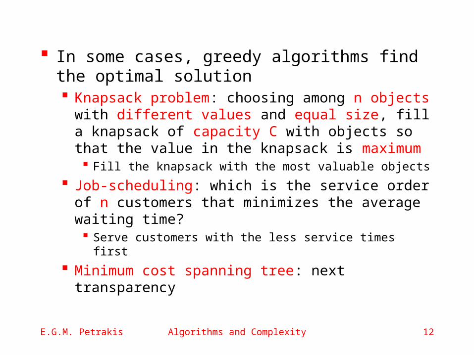
In some cases, greedy algorithms find the optimal solution Knapsack problem: choosing among n
objects with different values and equal size, fill a knapsack of capacity C with objects so that the value in the knapsack is maximum Fill the knapsack with the most valuable objects
Job-scheduling: which is the service order of n customers that minimizes the average waiting time? Serve customers with the less service times first
Minimum cost spanning tree: next transparency
E.G.M. Petrakis Algorithms and Complexity 13
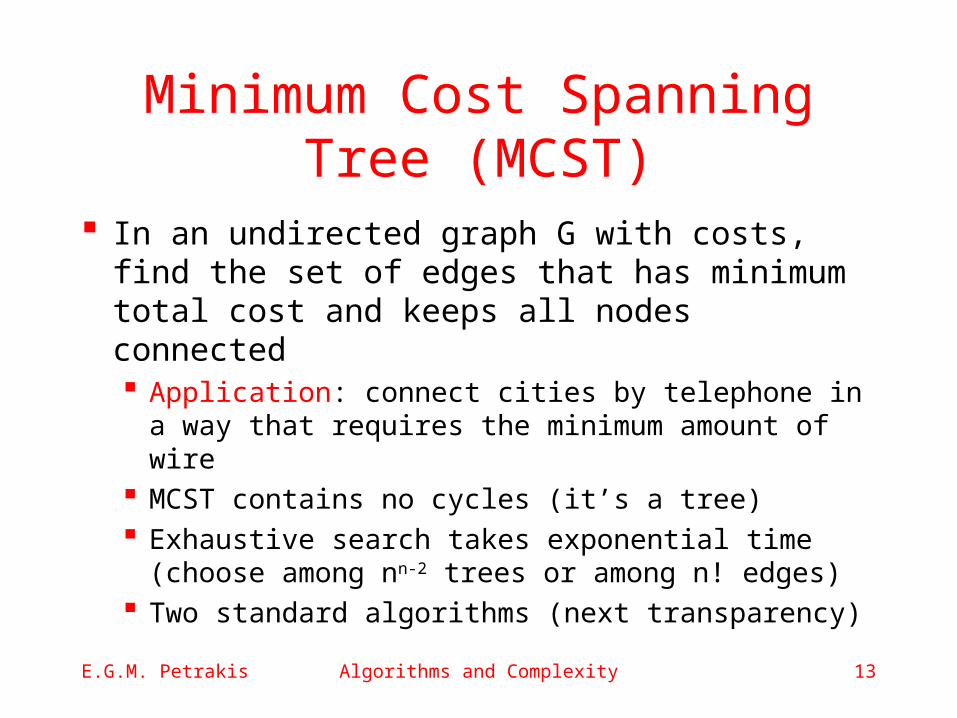
Minimum Cost Spanning Tree (MCST)
In an undirected graph G with costs, find the set of edges that has minimum total cost and keeps all nodes connected Application: connect cities by telephone in a
way that requires the minimum amount of wire
MCST contains no cycles (it’s a tree) Exhaustive search takes exponential time
(choose among nn-2 trees or among n! edges) Two standard algorithms (next transparency)
E.G.M. Petrakis Algorithms and Complexity 14
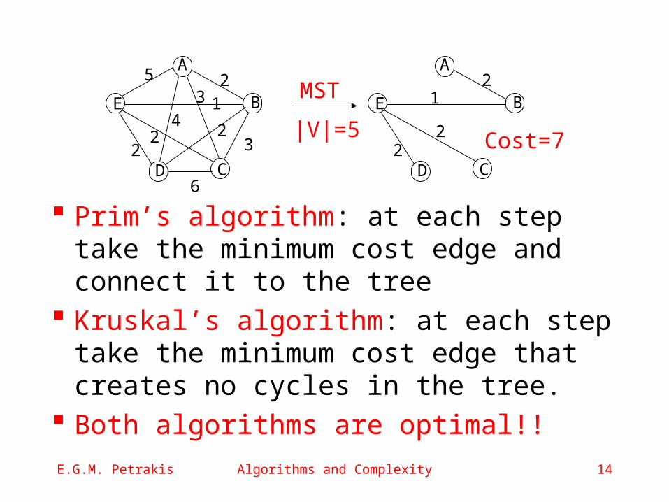
Prim’s algorithm: at each step take the minimum cost edge and connect it to the tree
Kruskal’s algorithm: at each step take the minimum cost edge that creates no cycles in the tree.
Both algorithms are optimal!!
Α
Ε
D
B
C
25
322 2
4
3 1
6
Α
Ε
D
B
C
2
22
1
|V|=5
MST
Cost=7
E.G.M. Petrakis Algorithms and Complexity 15
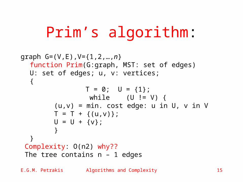
Prim’s algorithm:
graph G=(V,E),V={1,2,…,n} function Prim(G:graph, MST: set of edges)U: set of edges; u, v: vertices;{
T = 0; U = {1}; while (U != V) {
(u,v) = min. cost edge: u in U, v in VT = T + {(u,v)};U = U + {v};
}}
Complexity: O(n2) why?? The tree contains n – 1 edges
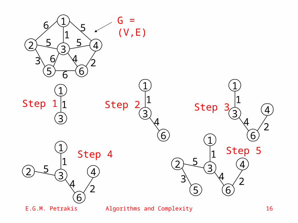
E.G.M. Petrakis Algorithms and Complexity 16
G = (V,E)
1
3
1
1
3
6
4
14
1
3
624
1
2 4
1
3
62
5
4
1
5
2 4
1
3
62
5
3 4
1
Step 1 Step 2 Step 3
Step 4 Step 5
5
2 4
1
3
6
6
2
5
55
3 6 4
1
6
E.G.M. Petrakis Algorithms and Complexity 17
Local Search
Heuristic algorithms that improve a non-optimal solution
Local transformation that improves a solution E.g., a solution obtained by a greedy algorithm
Apply many times and as long as the solution improves
Apply in difficult (NP problems) like TSP E.g., apply a greedy algorithm to obtain a solution,
improve this solution using local search The complexity of the transformation must be
polynomial
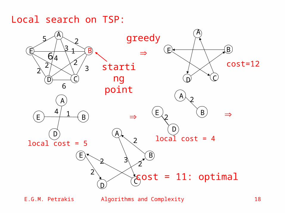
E.G.M. Petrakis Algorithms and Complexity 18
Α
Ε
D
B
C
25
322 2
4
3 1
6
starting point
greedy
B
Α
BΕ
D C
Α
Ε
D
B14
local cost = 5
Α
Ε
D
B
2
2
local cost = 4
Ε B
D
Α
C
2
2
2 32
cost = 11: optimal
Local search on TSP:
cost=126
E.G.M. Petrakis Algorithms and Complexity 19
Divide and Conquer
The problem is split into smaller sub-problems Solve the sub-problems Combine their solutions to obtain the solution
of the original problem The smaller a sub-problem is, the easier it is to
solve it Try to get sub-problems of equal size D&C is often expressed by recursive
algorithms E.g. Mergesort
E.G.M. Petrakis Algorithms and Complexity 20
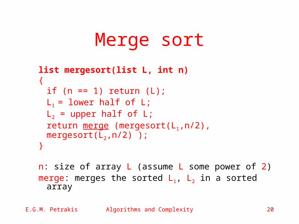
Merge sort
list mergesort(list L, int n) {
if (n == 1) return (L);L1 = lower half of L; L2 = upper half of L;return merge (mergesort(L1,n/2),
mergesort(L2,n/2) );}
n: size of array L (assume L some power of 2)merge: merges the sorted L1, L2 in a sorted array
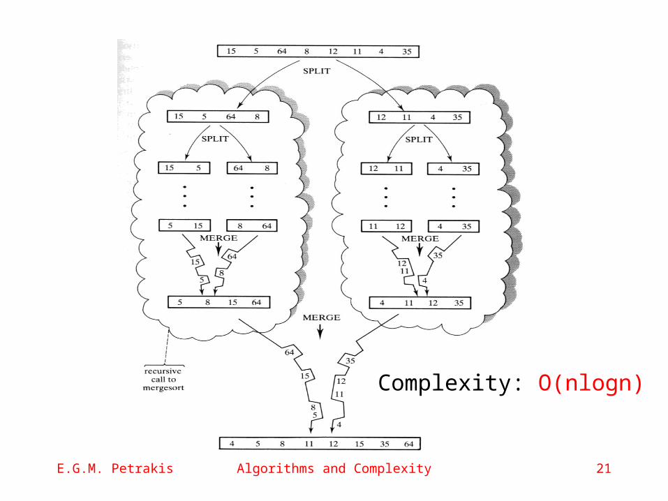
E.G.M. Petrakis Algorithms and Complexity 21
Complexity: O(nlogn)
E.G.M. Petrakis Algorithms and Complexity 22
Dynamic Programming
The original problem is split into smaller sub-problems Solve the sub-problems Store their solutions Reuse these solutions several times when
the same partial result is needed more than once in solving the main problem
DP is often based on a recursive formula for solving larger problems in terms of smaller
Similar to Divide and Conquer but recursion in D&C doesn’t reuse partial solutions
E.G.M. Petrakis Algorithms and Complexity 23
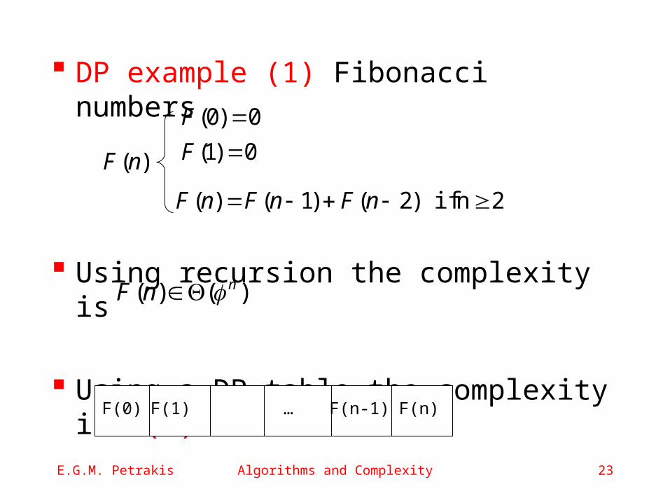
DP example (1) Fibonacci numbers
Using recursion the complexity is
Using a DP table the complexity is O(n)
)(nF 0)1(
0)0(
F
F
2n if )2()1()( nFnFnF
)()( nnF
F(0) F(1) F(n-1) F(n)…
E.G.M. Petrakis Algorithms and Complexity 24
0-1 Knapsack
0-1 knapsack problem: given a set of objects that vary in size and value, what is maximum value that can be carried in a knapsack of capacity C ??
How should we fill-up the capacity in order to achieve the maximum value?
E.G.M. Petrakis Algorithms and Complexity 25
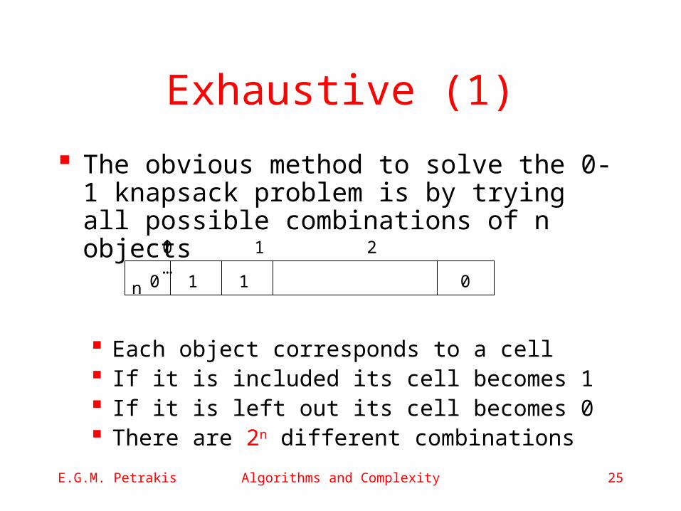
Exhaustive (1)
The obvious method to solve the 0-1 knapsack problem is by trying all possible combinations of n objects
Each object corresponds to a cell If it is included its cell becomes 1 If it is left out its cell becomes 0 There are 2n different combinations
0 1 2 … n
0 01 1
E.G.M. Petrakis Algorithms and Complexity 26
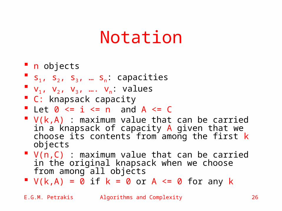
Notation
n objects s1, s2, s3, … sn: capacities v1, v2, v3, …. vn: values C: knapsack capacity Let 0 <= i <= n and A <= C V(k,A) : maximum value that can be carried in
a knapsack of capacity A given that we choose its contents from among the first k objects
V(n,C) : maximum value that can be carried in the original knapsack when we choose from among all objects
V(k,A) = 0 if k = 0 or A <= 0 for any k
E.G.M. Petrakis Algorithms and Complexity 27
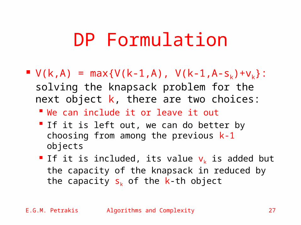
DP Formulation
V(k,A) = max{V(k-1,A), V(k-1,A-sk)+vk}: solving the knapsack problem for the next object k, there are two choices: We can include it or leave it out If it is left out, we can do better by choosing
from among the previous k-1 objects If it is included, its value vk is added but the
capacity of the knapsack in reduced by the capacity sk of the k-th object
E.G.M. Petrakis Algorithms and Complexity 28
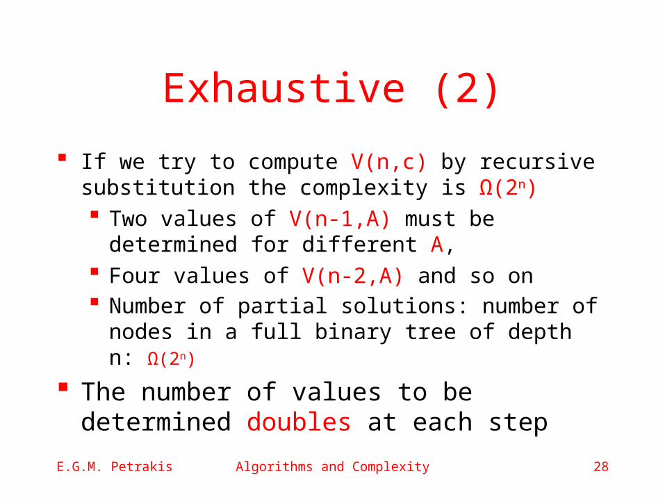
Exhaustive (2)
If we try to compute V(n,c) by recursive substitution the complexity is Ω(2n) Two values of V(n-1,A) must be determined
for different A, Four values of V(n-2,A) and so on Number of partial solutions: number of
nodes in a full binary tree of depth n: Ω(2n)
The number of values to be determined doubles at each step
E.G.M. Petrakis Algorithms and Complexity 29
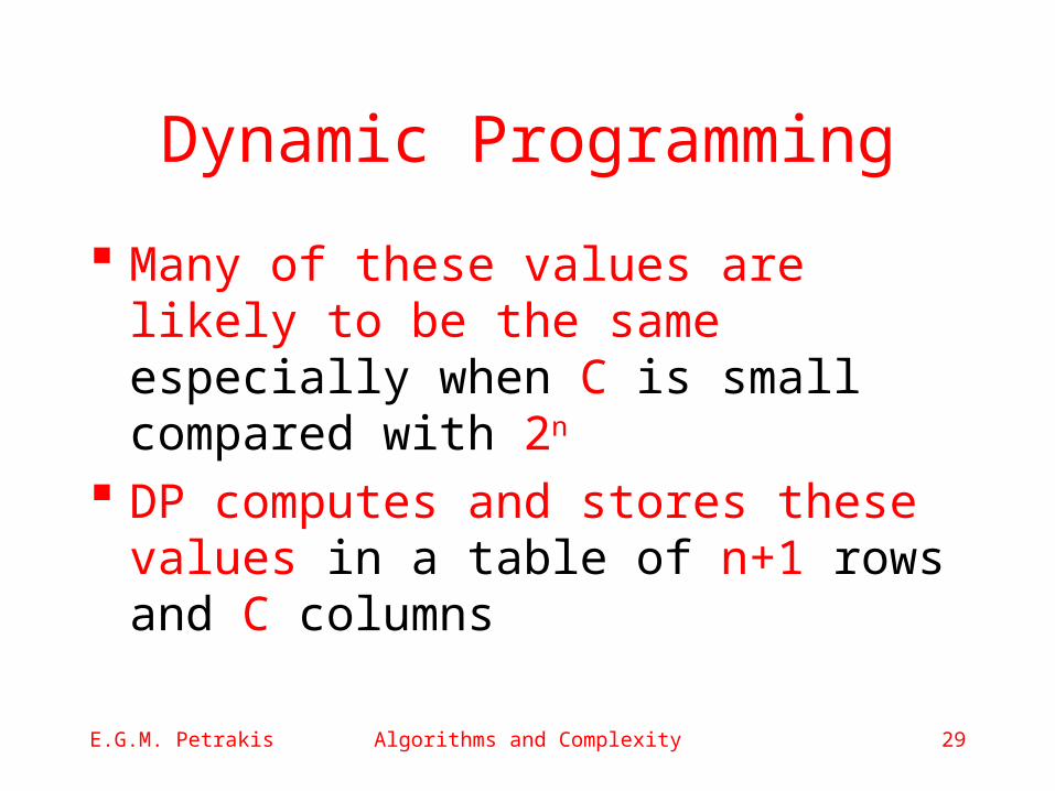
Dynamic Programming
Many of these values are likely to be the same especially when C is small compared with 2n
DP computes and stores these values in a table of n+1 rows and C columns
E.G.M. Petrakis Algorithms and Complexity 30
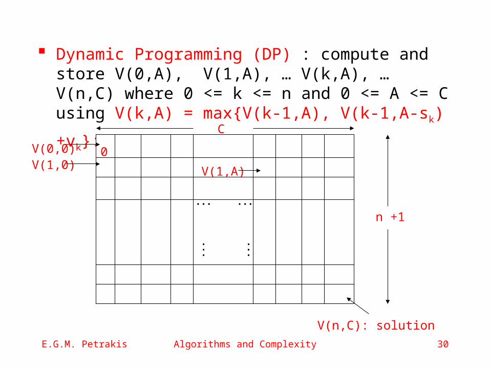
Dynamic Programming (DP) : compute and store V(0,A), V(1,Α), … V(k,A), … V(n,C) where 0 <= k <= n and 0 <= A <= C using V(k,A) =
max{V(k-1,A), V(k-1,A-sk)+vk}:
V(n,C): solution
C
0V(0,0)V(1,0) V(1,A)
n +1
E.G.M. Petrakis Algorithms and Complexity 31
DP on Knapsack
Each partial solution V(k,A) takes constant time to compute
The entire table is filled with values The total time to fill the table is proportional to
its size => the complexity of the algorithm is O(nC) Faster than exhaustive search if C << 2n
Which objects are included? Keep this information in a second table Xi(k,A)
Xi(k,A) = 1 if object i is included, 0 otherwise
E.G.M. Petrakis Algorithms and Complexity 32
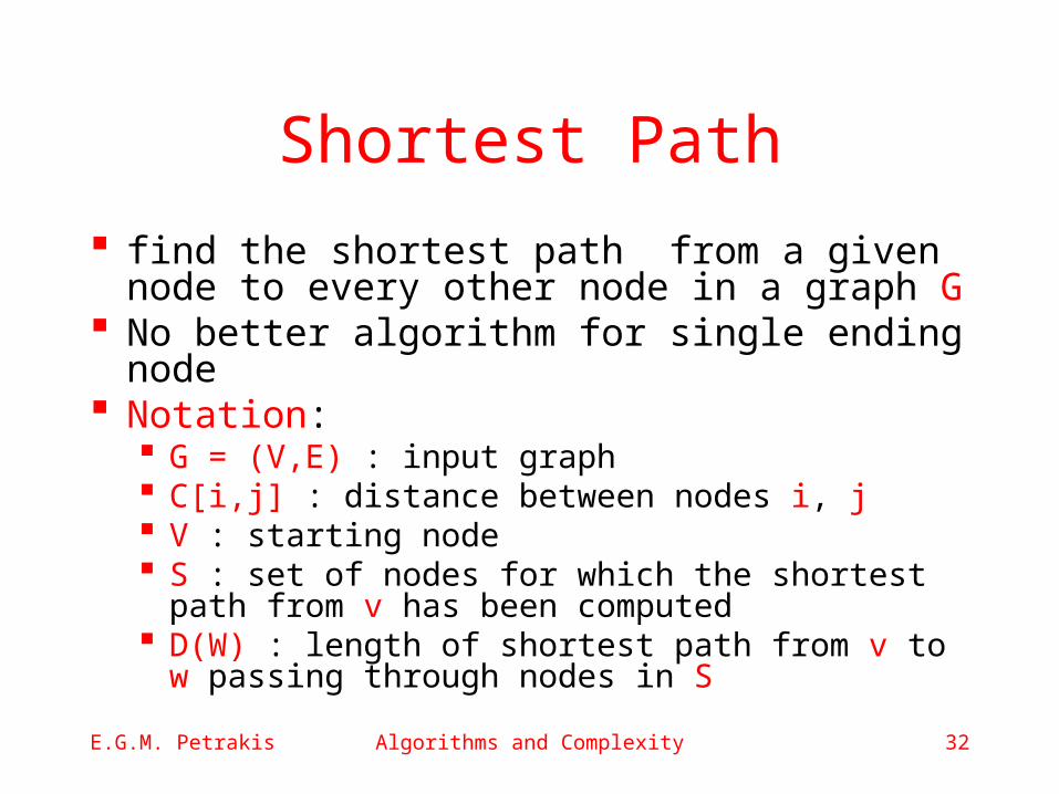
Shortest Path
find the shortest path from a given node to every other node in a graph G
No better algorithm for single ending node
Notation: G = (V,E) : input graph C[i,j] : distance between nodes i, j V : starting node S : set of nodes for which the shortest path
from v has been computed D(W) : length of shortest path from v to w
passing through nodes in S
E.G.M. Petrakis Algorithms and Complexity 33
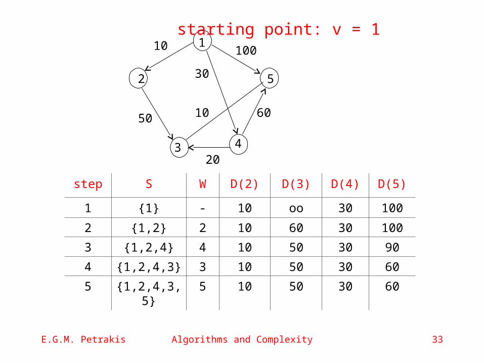
20
1
2
3
5
4
10010
6050 10
30
starting point: v = 1
step S W D(2) D(3) D(4) D(5)
1 {1} - 10 oo 30 100
2 {1,2} 2 10 60 30 100
3 {1,2,4} 4 10 50 30 90
4 {1,2,4,3} 3 10 50 30 60
5 {1,2,4,3,5}
5 10 50 30 60
E.G.M. Petrakis Algorithms and Complexity 34
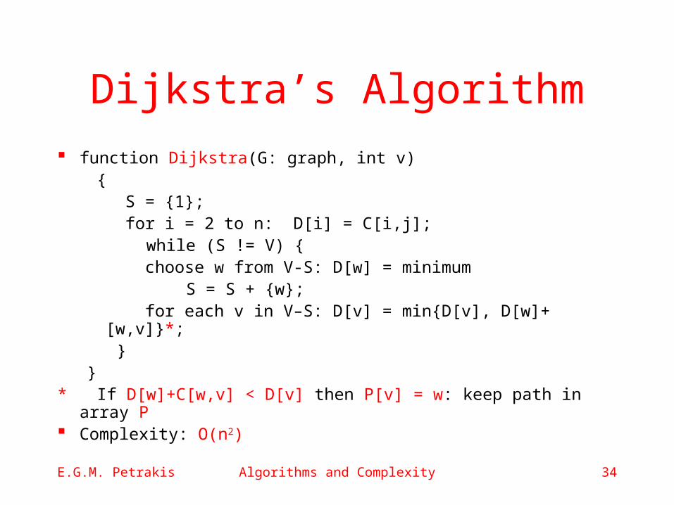
Dijkstra’s Algorithm function Dijkstra(G: graph, int v) {
S = {1}; for i = 2 to n: D[i] = C[i,j];
while (S != V) { choose w from V-S: D[w] = minimum
S = S + {w}; for each v in V–S: D[v] = min{D[v], D[w]+
[w,v]}*; }}
* If D[w]+C[w,v] < D[v] then P[v] = w: keep path in array P Complexity: O(n2)
E.G.M. Petrakis Algorithms and Complexity 35
DP on TSP
The standard algorithm is Ω((n-1)!) If the same partial paths are used many
times then DP can be faster! Notation:
Number the cities 1,2,…n, 1 is the starting-ending point d(i,j) : distance from node i to j D(b,S) : length of shortest path that starts at
b visits all cities in S in some order and ends at node 1
S is subset of {1,2,…n} – {1,b}
E.G.M. Petrakis Algorithms and Complexity 36
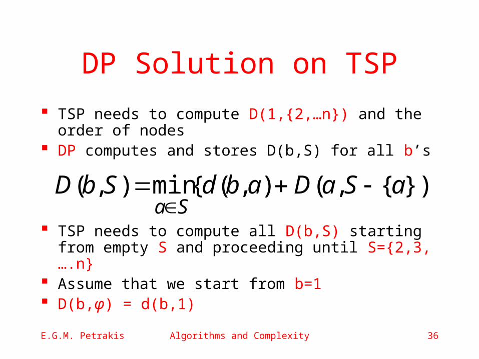
DP Solution on TSP
TSP needs to compute D(1,{2,…n}) and the order of nodes
DP computes and stores D(b,S) for all b’s
TSP needs to compute all D(b,S) starting from empty S and proceeding until S={2,3,….n}
Assume that we start from b=1 D(b,φ) = d(b,1)
})}{,(),({min),( aSaDabdSbDSa
E.G.M. Petrakis Algorithms and Complexity 37
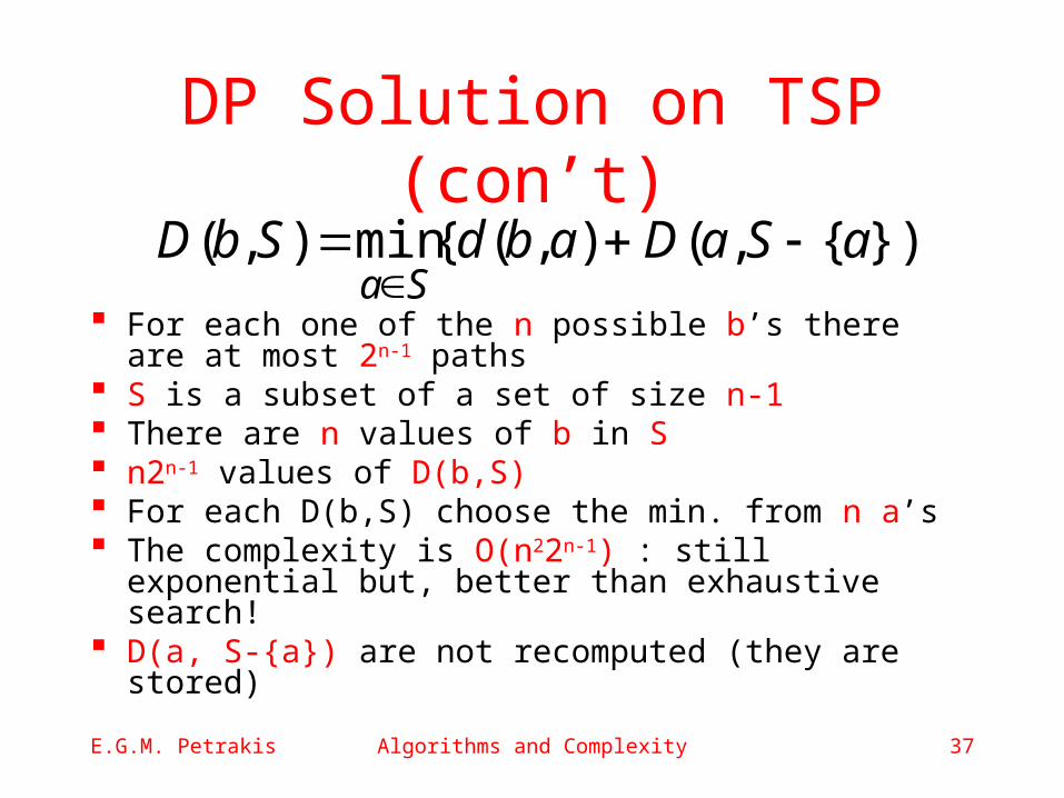
DP Solution on TSP (con’t)
For each one of the n possible b’s there are at most 2n-1 paths
S is a subset of a set of size n-1 There are n values of b in S n2n-1 values of D(b,S) For each D(b,S) choose the min. from n a’s The complexity is O(n22n-1) : still exponential
but, better than exhaustive search! D(a, S-{a}) are not recomputed (they are
stored)
})}{,(),({min),( aSaDabdSbDSa
E.G.M. Petrakis Algorithms and Complexity 38
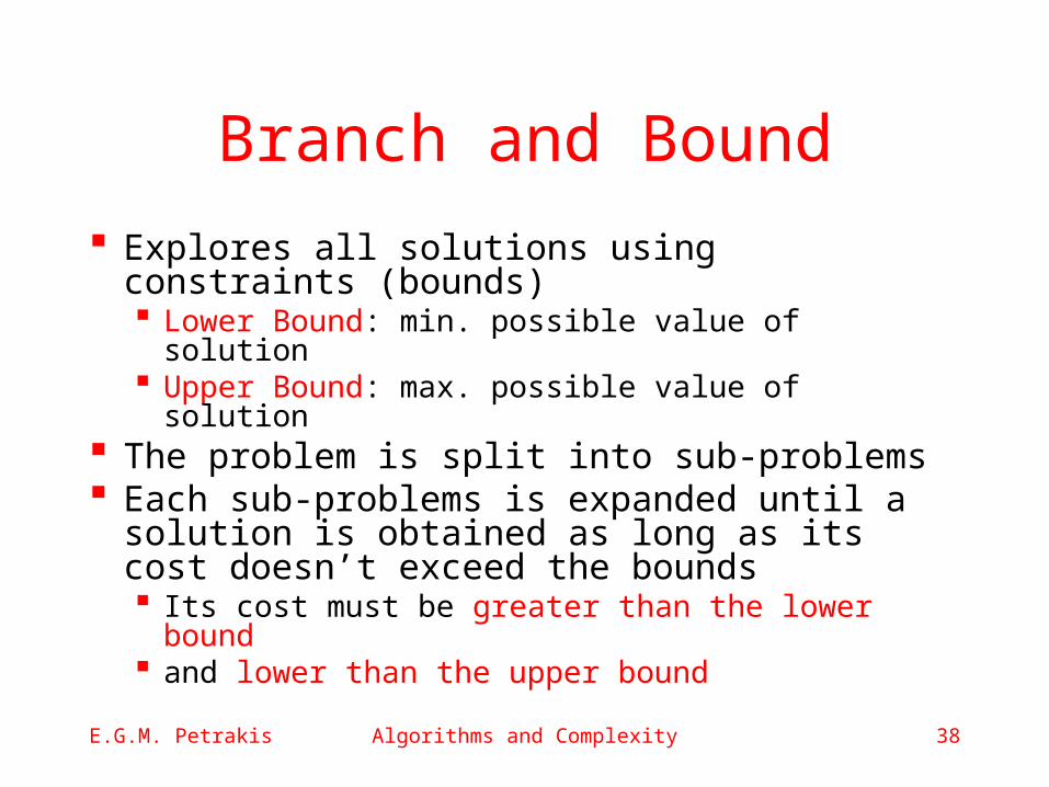
Branch and Bound
Explores all solutions using constraints (bounds) Lower Bound: min. possible value of solution Upper Bound: max. possible value of solution
The problem is split into sub-problems Each sub-problems is expanded until a
solution is obtained as long as its cost doesn’t exceed the bounds Its cost must be greater than the lower bound and lower than the upper bound
E.G.M. Petrakis Algorithms and Complexity 39
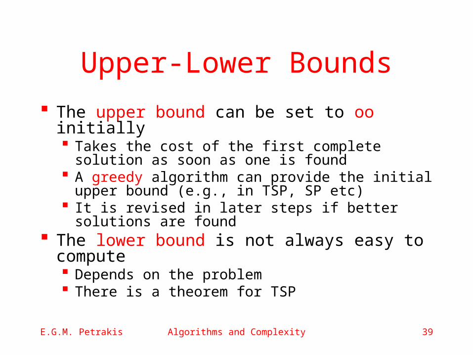
Upper-Lower Bounds
The upper bound can be set to oo initially Takes the cost of the first complete solution
as soon as one is found A greedy algorithm can provide the initial
upper bound (e.g., in TSP, SP etc) It is revised in later steps if better solutions
are found The lower bound is not always easy to
compute Depends on the problem There is a theorem for TSP
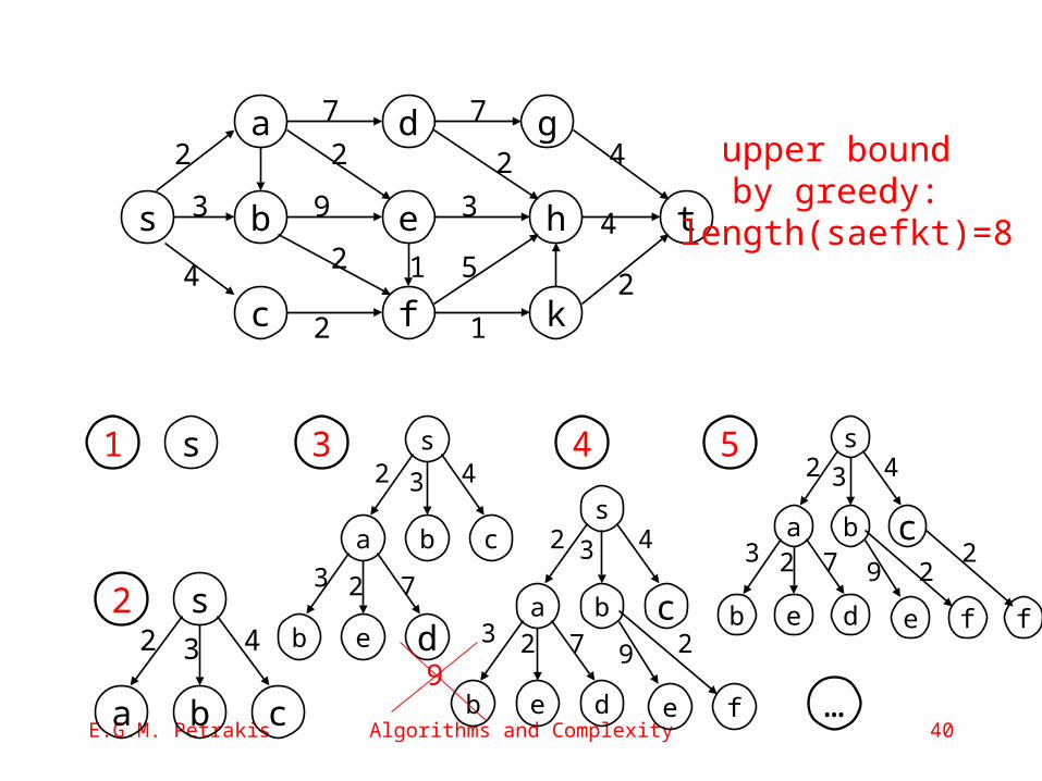
E.G.M. Petrakis Algorithms and Complexity 40
s
c f
a d
e
g
h
k
tb1
1
2 2
2
2
2
2
4
4
4
3 39
5
7 7
s
s
a b c
2 3 4
1
2
3 s
b ca
b e d
2 3 4
3 2 7
4
s
b ca
b e d e f
2 3 4
3 2 7 9 2
5 s
b ca
b e d e f
2 3 4
3 2 7 9 2
f
2
…
upper bound by greedy:
length(saefkt)=8
9
E.G.M. Petrakis Algorithms and Complexity 41
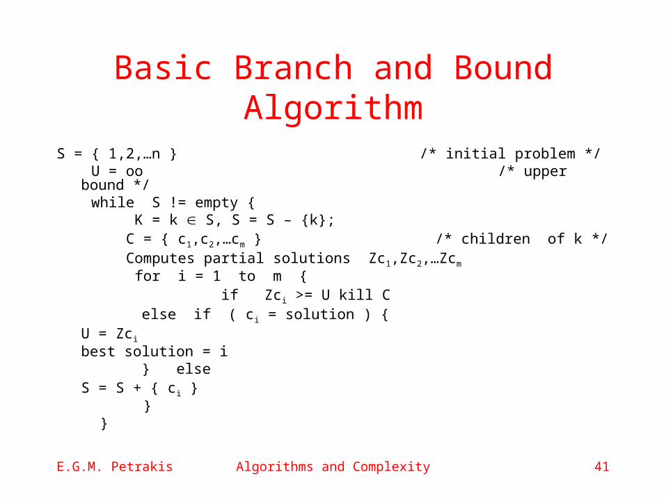
Basic Branch and Bound Algorithm
S = { 1,2,…n } /* initial problem */ U = oo /* upper bound */ while S != empty { K = k S, S = S – {k}; C = { c1,c2,…cm } /* children of k */ Computes partial solutions Zc1,Zc2,…Zcm
for i = 1 to m { if Zci >= U kill C
else if ( ci = solution ) {U = Zci
best solution = i } else
S = S + { ci } } }
![Algorithmic problems in the research of number … Las Vegas type randomized algorithm, which produces an expansive polynomial in R[x], then makes round. Using the algorithm of Dufresnoy](https://static.fdocument.org/doc/165x107/5b927d8e09d3f232708be49a/algorithmic-problems-in-the-research-of-number-las-vegas-type-randomized-algorithm.jpg)