Effects of Different Influence Factors on Static and ...ijetch.org/vol7/774-G3011.pdfthat influence...

Abstract—Many analytic factors affect predicted results of

mooring line’s static and dynamic responses associated with the platform motions. The paper presents a study of analytic factors that influence static and dynamic responses of a mooring line. These factors include mooring line characteristics, environmental conditions, and external excitations such as platform motions. In this paper, a finite element model for a mooring line system is built for a comparative study on computational efficiency and convergence of different initial values for static analysis. The paper also presents investigation of mooring line dynamic responses under different environmental conditions and external excitations, and discusses various influences of the above mentioned factors on the mooring line dynamic tension. Some conclusions are drawn, which can be the reference for mooring line design and analysis.

Index Terms—Mooring line, dynamic analysis, finite element model, slender rod theory.

I. INTRODUCTION There are primarily three types of models for mooring line

analysis: 1) catenary model, 2) lumped mass model, and 3) finite element model [1]. The traditional catenary model has various restrictions in use because of too many assumed conditions applied, in particular, when the environment loads can not be neglected [2]. The lumped mass method concentrates mass and external forces to nodes that are located at the ends of each segment. The nodes are then connectted by zero-mass spring that can simulate elongation and elastic stiffness. However, for a system with multiple mooring lines, the lumped mass method appears inopportune for programming [3]. The finite element model thus becomes ever more popular. Garrett advanced a three-dimensional elastic rod finite element model, in which elements are of linear elasticity and torsion is neglected [4]. The elastic rod method has been widely used in the analysis of a slender such as mooring line, riser and pipeline.

In this paper, based on the elastic rod theory, the non-linear finite element method was adopted for analyzing static and dynamic responses of a mooring line in cooresponding to environment loads and external excitations. The paper first discusses computational efficiency and convergence of

Manuscript received February 28, 2014; revise April 28, 2014. This work

was supported by the Programme of Introducing Talents of Discipline to Universities (Grant No. B07019), the Fundamental Research Funds for the Central Universities (Grant No. HEUCF140119), the Research Foundation for the Doctoral Program of Higher Education of China (Grant No. 20132304120008).

The authors are with the Harbin Engineering University, China (e-mail: [email protected], [email protected], [email protected], [email protected]).

different initial values for static analysis, and also investigates the mooring line dynamic response under different environmental conditions and external excitations.

II. SLENDER ROD THEORY In Garrett’s slender rod theory, the behavior of the rod is

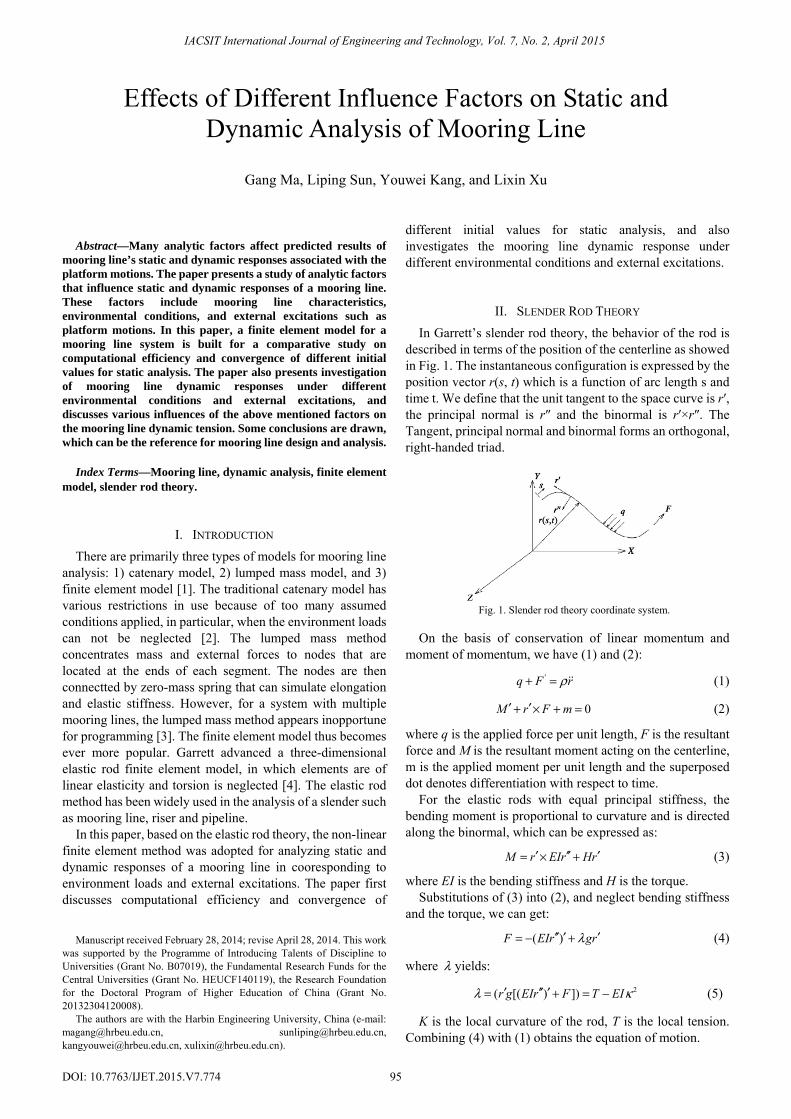
described in terms of the position of the centerline as showed in Fig. 1. The instantaneous configuration is expressed by the position vector r(s, t) which is a function of arc length s and time t. We define that the unit tangent to the space curve is r′, the principal normal is r″ and the binormal is r′×r″. The Tangent, principal normal and binormal forms an orthogonal, right-handed triad.

Fig. 1. Slender rod theory coordinate system.

On the basis of conservation of linear momentum and

moment of momentum, we have (1) and (2): 'q F rρ+ = (1)

0M r F m′ ′+ × + = (2)

where q is the applied force per unit length, F is the resultant force and M is the resultant moment acting on the centerline, m is the applied moment per unit length and the superposed dot denotes differentiation with respect to time.

For the elastic rods with equal principal stiffness, the bending moment is proportional to curvature and is directed along the binormal, which can be expressed as:

M r EIr Hr′ ′′ ′= × + (3)

where EI is the bending stiffness and H is the torque. Substitutions of (3) into (2), and neglect bending stiffness

and the torque, we can get:

( )F EIr grλ′′ ′ ′= − + (4)

where λ yields: 2( [( ) ])r g EIr F T EIλ κ′ ′′ ′= + = − (5)

K is the local curvature of the rod, T is the local tension. Combining (4) with (1) obtains the equation of motion.

Effects of Different Influence Factors on Static and Dynamic Analysis of Mooring Line

Gang Ma, Liping Sun, Youwei Kang, and Lixin Xu

95

IACSIT International Journal of Engineering and Technology, Vol. 7, No. 2, April 2015

DOI: 10.7763/IJET.2015.V7.774

( )EIr gr q rλ ρ′′ ′′ ′− + + = (6)

And the stretch constrained equation:

* 1 2 Tr rEA

′ ′ = + (7)

III. NUMERICAL IMPLEMENTATION In this paper, a finite element solution method is employed

to discrete the vector governing equations into algebraic equations. The method, based on the Galerkin method, uses a set of shape functions to approximate the cable and the variations of the tensions (and other parameters) along it. Then we use the Newton method to solve the static problem and Adams-Moulton method for the dynamic problem.

A. Discretization of the Governing Equations As we can see from (6), the governing equation is a high

order partial differential equation, so the Galerkin method is adopted to solve this problem [5]. By the use of shape functions, unknowns in the equation can be approximated as:

( , ) ( ) ( )( , ) ( ) ( )( , ) ( ) ( )

in i n

m m

mn m n

r s t U t a s es t t p s

q s t q t p s eλ λ

===

(8)

where, ( )ia s and ( )mp s are shape functions, ( )inU t , ( )m tλ ,

( )q tmn represent the nodal and mid-section values. Multiplying both side of the equation with a(s) and

integrating it with respect to s from 0 to L for a segment (or an element) of the rod with length L:

{ }0

( ) ( ) 0L

ir EIr r q a s dsρ λ′′ ′′ ′+ − − =∫ (9)

We obtain the discrete form of the equation of motion for

an element of a rod with length L:

ikm m kn ikm m kn ikm m kn im mnM U B U U qγ α β λ μ+ + = (10) where:

1

301

0

1

0

1

0

1 ( ) ( ) ( )

1 ( ) ( ) ( )

( ) ( ) ( )

( ) ( )

ikm i k m

ikm i k m

ikm i k m

im i m

a a p dL

a a p dL

L a a p d

L a p d

α ξ ξ ξ ξ

β ξ ξ ξ ξ

γ ξ ξ ξ ξ

μ ξ ξ ξ

′′ ′′=

′ ′=

=

=

∫

∫

∫

∫

Similarly, we obtain the discrete form of (7)

{ }1 1 22 2ikm in kn m km kU Uβ τ η ε= + (11)

In which:

1

01

0

( ) ( )

( )

lm l m

m m

L p p d

L p d

η ξ ξ ξ

τ ξ ξ

=

=

∫

∫

B. Newton Method for the Static Analysis For the static problem, all the terms related to the time

derivatives are zero, so (10) is reduced to:

ikm m kn ikm m kn im mnB U U qα β λ μ+ = (12)

The fixed-point Newton iteration method is utilized to solve the equations. Let 0U and 0λ be a first guess, then the new values of U and λ are

0

0

kn kn kn

m m m

U U Uδλ λ δλ

= +

= + (13)

Plugging the new expression of U and λ into (11) and

(12), and discarding all the high order terms, the static problem to be solved is then represented by the following equations:

0 0

0 0 0Uλ+

= −ikm m kn ikm m kn ikm m kn

im mn ikm m kn ikm m kn

α B δU β λ δU + β δλ U

μ q - α B U β (14)

0

ll

0 0 0

( ) }

1 ( 2 )2

−

=

ikm in kn lm f f i it t

m lm l ikm in kn

δλ δyβ U δU - η { g ρ A - ρ AA E A E

τ + η ε - β U U

(15)

The static control equation is a group of linear equations, in which knUδ and mδλ are the unknowns. If the number of segments is N, then the dimension of whole matrix equations for mooring line should be 15+8(N-1). The entire matrix equations iterate as (13) repeatedly until knUδ and mδλ are small enough, then the steady static solutions are obtained.

C. Adams Method for the Dynamic Analysis The basic thought of linear multistep method is: take full

advantage of the known quantities like 0y to ny to forecast 1ny + in the steps of solve the equation. One of the

methods acts like 10

k

n k n k i n ii

y y h fβ+ + − +=

= + ∑ is named as

Adams method [6]. If 0kβ = , we call it explicit method, and while 0kβ ≠ , we call it implicit method.

The Adams-Moulton method (the implicit method) is adopted to solve the dynamic problem. As did in the static problem, we conclude that the dynamic equation of the motion of a rod is of the form MU c= , where vector

im mn ikm m kn ikm m knc q B U Uμ α β λ= − − consists of all the terms which are not time derivatives.

Let h be time step from t=n to t=n+1. We can approximately represent ,M U and c by:

96


( 1) ( )

( 1) ( )2

2

kk

n ni i

i

n nm m

m

uuh

c cc

M MM

δ

+

+

=

+=

+=

(16)

where Taylor's expansion was employed to obtain the values at t = n+1:

1( )( 1) ( ) ( )2

1 1( ) ( )( 1) ( ) ( ) ( )2 211 12

nn n nm m mk k

n nn n n ni i ik k im m

M M J u

c c K u K

δ

δ δλ

++

+ ++

= +

= + + (17)

where:

1( )2

nm

mkk

MJu

+ ∂=∂ ,

1( ) ( ) ( 1)2 1 (3 )2

n n nm m mλ λ λ

+ −= −

1 1( ) ( )2 2

11

n niik ikm m ikm m

k

cK Bu

α β λ+ +∂= = − −

∂

1 1( ) ( )2 2

12 kn

n niim ikm

m

cK Uβλ

+ +∂= = −∂ ,

1( ) ( ) ( )2

2n n n

k k khu u u

+= +

Then the equation can be written as:

1( )12 ( )2( ) ( ) ( )211

1 12 ( ) ( )( ) ( ) ( )2 212 112

1( )4 2

24 2

n nn n nmk kik ikm m k

n nn n nim m i ik k

h J u hK M uh

h hK c K uh

γ δ

δλ

++

+ +

⎧ ⎫⎪ ⎪⎧ ⎫− + + +⎨ ⎬⎨ ⎬

⎩ ⎭⎪ ⎪⎩ ⎭⎧ ⎫⎪ ⎪⎧ ⎫− = +⎨ ⎬⎨ ⎬

⎩ ⎭⎪ ⎪⎩ ⎭

(18)

Similarly we can transform the stretch equation, and it can be expanded to be of the form:

1 12 2( ) ( )( ) ( )2 221 22 2

( ) 1( ) ( )221

1 24 4

2 2

n nn njk k jm m

nnj n

jk k

h hK u Kh h

d h K u

δ δλ+ +

+

⎧ ⎫ ⎧ ⎫⎪ ⎪ ⎪ ⎪⎧ ⎫ ⎧ ⎫− + −⎨ ⎬⎨ ⎬ ⎨ ⎬⎨ ⎬⎩ ⎭ ⎩ ⎭⎪ ⎪ ⎪ ⎪⎩ ⎭ ⎩ ⎭

= +

(19)

where:

1 1( ) ( )2 2

21 kn

n njjk ikm

k

dK U

uβ

+ +∂= = −

∂ ,1( )2

22

n j kmjm

m

dK

EAη

λ+ ∂

= =∂

Equation (17) and (18) are solved to obtain the increment

of the generalized velocity u , and the effective tension λ . The values of u and λ at the new time are obtained by the following approach:

{ }( 1) ( ) ( ) ( )22

( 1) ( ) ( )

hn n n nu u u uk kk kn n n

m m m

δ

λ λ δλ

+ = + +

+ = + (20)

The values of u and λ at time t = n+1 serve as a starting point for the next calculation.

IV. MODEL FOR STATIC ANALYSIS The catenary model is a physical model which has an

accurate analytical solution. In order to verify the feasibility of the program, we compare the result with catenary analytical solution. Then a discussion on the effects of different initial values on static analysis efficiency and stability was made, with the purpose of choosing a reasonable initial value.

Take mooring line parameters for static analysis as follow:

TABLE I: MOORING LINE PARAMETERS Property item Value

Water depth(m) 120 G (m/s2) 9.8

Mass(kg/m) 1.35350E+02 E（Pa） 5.51090E+10

Cross area(m2) 9.07292E-03 Length(m) 1200

Diameter(m) 7.60000E-02 Buoyancy(N/m) 1.70171E+02

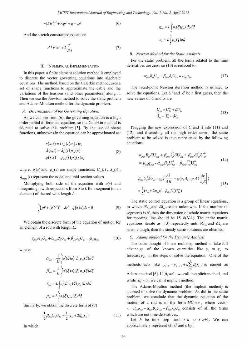
The catenary model has some parts with contact with the

seabed, and this can verify the seabed boundary condition. The figure below is the comparison of catenary model and the slender rod model.

Fig. 2. Static configuration of mooring line.

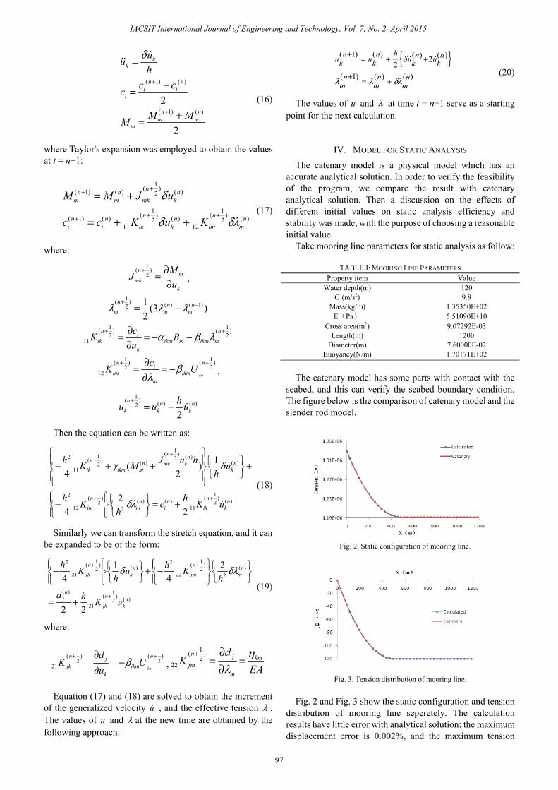
Fig. 3. Tension distribution of mooring line.

Fig. 2 and Fig. 3 show the static configuration and tension

distribution of mooring line seperetely. The calculation results have little error with analytical solution: the maximum displacement error is 0.002%, and the maximum tension

97


error is 0.002%. Therefore, the slender rod theory can get the displacement and force of static mooring line accurately.

V. DISCUSSION ABOUT INITIAL VALUES FOR STATIC ANALYSIS

Before static analysis we should have the initial value of mooring line, including: positions and pretension for each nodes, etc. In this paper, we choose three different initial values for the static analysis and the contrastive analysis between them.

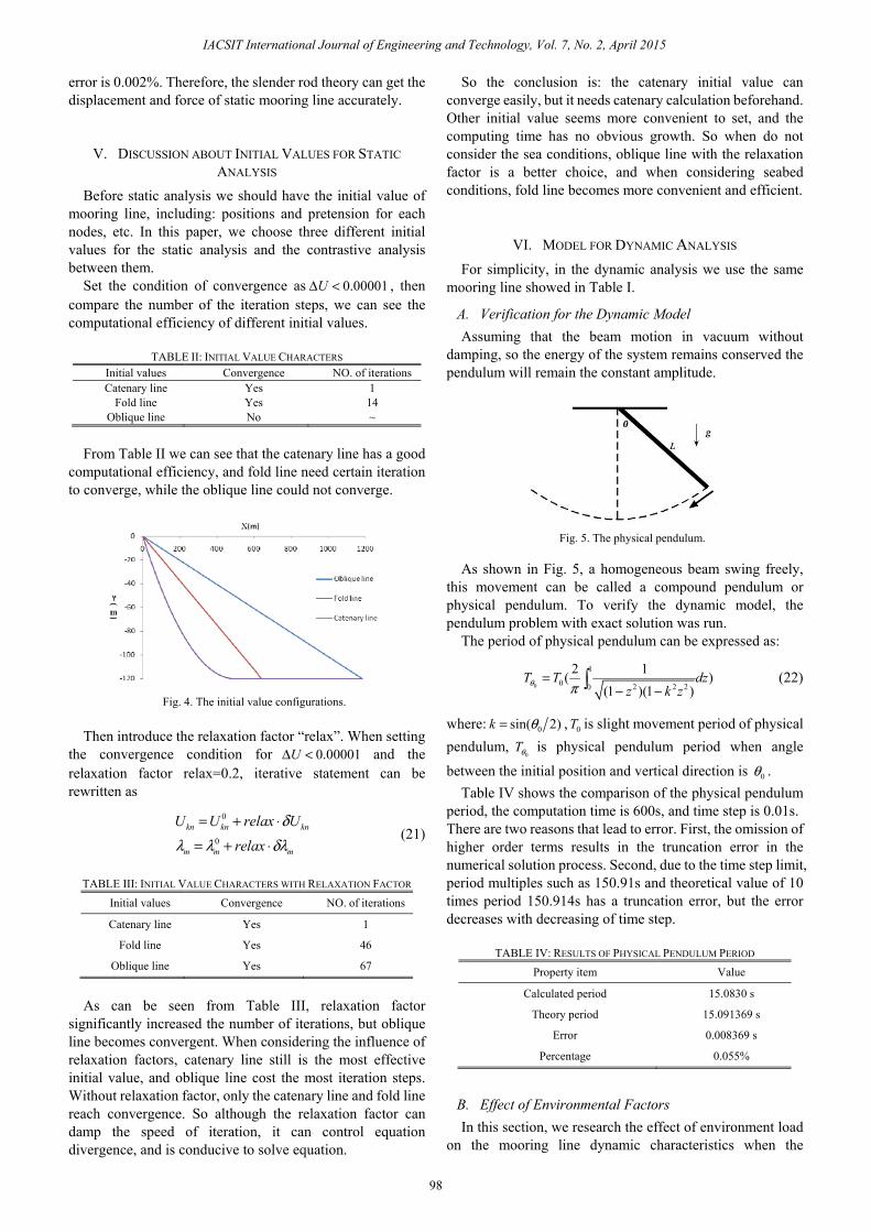
Set the condition of convergence as 0.00001UΔ < , then compare the number of the iteration steps, we can see the computational efficiency of different initial values.

TABLE II: INITIAL VALUE CHARACTERS

Initial values Convergence NO. of iterationsCatenary line Yes 1

Fold line Yes 14 Oblique line No ~

From Table II we can see that the catenary line has a good

computational efficiency, and fold line need certain iteration to converge, while the oblique line could not converge.

Fig. 4. The initial value configurations.

Then introduce the relaxation factor “relax”. When setting

the convergence condition for 0.00001UΔ < and the relaxation factor relax=0.2, iterative statement can be rewritten as

0

0

kn kn kn

m m m

U U relax U

relax

δλ λ δλ

= + ⋅

= + ⋅ (21)

TABLE III: INITIAL VALUE CHARACTERS WITH RELAXATION FACTOR

Initial values Convergence NO. of iterations

Catenary line Yes 1

Fold line Yes 46

Oblique line Yes 67

As can be seen from Table III, relaxation factor

significantly increased the number of iterations, but oblique line becomes convergent. When considering the influence of relaxation factors, catenary line still is the most effective initial value, and oblique line cost the most iteration steps. Without relaxation factor, only the catenary line and fold line reach convergence. So although the relaxation factor can damp the speed of iteration, it can control equation divergence, and is conducive to solve equation.

So the conclusion is: the catenary initial value can converge easily, but it needs catenary calculation beforehand. Other initial value seems more convenient to set, and the computing time has no obvious growth. So when do not consider the sea conditions, oblique line with the relaxation factor is a better choice, and when considering seabed conditions, fold line becomes more convenient and efficient.

VI. MODEL FOR DYNAMIC ANALYSIS

For simplicity, in the dynamic analysis we use the same mooring line showed in Table I.

A. Verification for the Dynamic Model Assuming that the beam motion in vacuum without

damping, so the energy of the system remains conserved the pendulum will remain the constant amplitude.

Fig. 5. The physical pendulum.

As shown in Fig. 5, a homogeneous beam swing freely,

this movement can be called a compound pendulum or physical pendulum. To verify the dynamic model, the pendulum problem with exact solution was run.

The period of physical pendulum can be expressed as:

0

1

0 2 2 20

2 1( )(1 )(1 )

T T dzz k z

θ π=

− −∫ (22)

where: 0sin( 2)k θ= , 0T is slight movement period of physical pendulum,

0Tθ is physical pendulum period when angle

between the initial position and vertical direction is 0θ . Table IV shows the comparison of the physical pendulum

period, the computation time is 600s, and time step is 0.01s. There are two reasons that lead to error. First, the omission of higher order terms results in the truncation error in the numerical solution process. Second, due to the time step limit, period multiples such as 150.91s and theoretical value of 10 times period 150.914s has a truncation error, but the error decreases with decreasing of time step.

TABLE IV: RESULTS OF PHYSICAL PENDULUM PERIOD Property item Value

Calculated period 15.0830 s

Theory period 15.091369 s

Error 0.008369 s

Percentage 0.055%

B. Effect of Environmental Factors In this section, we research the effect of environment load

on the mooring line dynamic characteristics when the

98


mooring line experiences top disturbance. The upper end excitation is sinusoidal excitation in horizontal direction: ( ) 2sin(0.6 )X t t= . And the displacement curve shows in Fig. 6.

Fig. 6. Horizontal force-displacement curve.

Fig. 7. Variation tension at the mooring line’s upper end.

As can be seen from Fig. 7, the tension changes in the

equivalent frequency with external excitation and its amplitude flapping up and down cross the static tension. The mooring line keeps in tension, and does not appear relaxation.

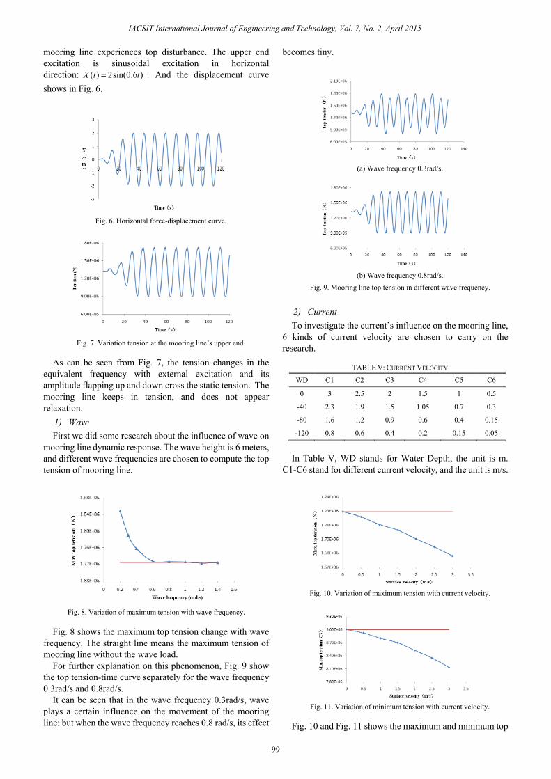
1) Wave First we did some research about the influence of wave on

mooring line dynamic response. The wave height is 6 meters, and different wave frequencies are chosen to compute the top tension of mooring line.

Fig. 8. Variation of maximum tension with wave frequency.

Fig. 8 shows the maximum top tension change with wave

frequency. The straight line means the maximum tension of mooring line without the wave load.

For further explanation on this phenomenon, Fig. 9 show the top tension-time curve separately for the wave frequency 0.3rad/s and 0.8rad/s.

It can be seen that in the wave frequency 0.3rad/s, wave plays a certain influence on the movement of the mooring line; but when the wave frequency reaches 0.8 rad/s, its effect

becomes tiny.

(a) Wave frequency 0.3rad/s.

(b) Wave frequency 0.8rad/s.

Fig. 9. Mooring line top tension in different wave frequency. 2) Current To investigate the current’s influence on the mooring line,

6 kinds of current velocity are chosen to carry on the research.

TABLE V: CURRENT VELOCITY

WD C1 C2 C3 C4 C5 C6

0 3 2.5 2 1.5 1 0.5

-40 2.3 1.9 1.5 1.05 0.7 0.3

-80 1.6 1.2 0.9 0.6 0.4 0.15

-120 0.8 0.6 0.4 0.2 0.15 0.05

In Table V, WD stands for Water Depth, the unit is m.

C1-C6 stand for different current velocity, and the unit is m/s.

Fig. 10. Variation of maximum tension with current velocity.

Fig. 11. Variation of minimum tension with current velocity.

Fig. 10 and Fig. 11 shows the maximum and minimum top

99


tension of mooring line separately. The straight line stands for the maximum and minimum top tension without current loads. As can be seen, the maximum and minimum top tensions decrease with the increase of current velocity. This illustrates that, under external excitation, the current acts like a quasi-static force and has damping effect to the mooring line on certain extent, and the damping effect becomes manifest when the current velocity increase.

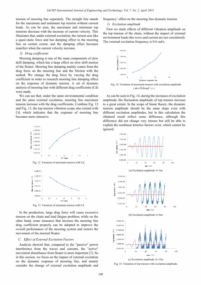
3) Drag coefficients Mooring damping is one of the main components of slow

drift damping, which has a large effect on slow drift motion of the floater. Mooring line damping mainly comes from the drag force on the mooring line and the friction with the seabed. We change the drag force by varying the drag coefficient in order to research mooring line damping effect on the response of dynamic tension. A set of dynamic analysis of mooring line with different drag coefficients (Cd) were made.

We can see that, under the same environmental condition and the same external excitation, mooring line maximum tension increase with the drag coefficients. Combine Fig. 12 and Fig. 13, the top tension vibration scope also extend with Cd, which indicates that the response of mooring line becomes more intensive.

Fig. 12. Variation of maximum tension with Cd.

Fig. 13. Variation of minimum tension with Cd.

In the production, large drag force will cause excessive

tension on the chain and lead fatigue problem; while on the other hand, some measures that increase the mooring line drag coefficient properly can be adopted to improve the overall performance of the mooring system and restrict the movement of the moored floater.

C. Effect of External Excitation Factors Analysis showed that, compared to the "passive" power

interference from the waves and currents, the "active" movement disturbance from floater is more important [7]. So in this section, we focus on the impact of external excitation on the dynamic response of mooring line, and mainly consider the change of external excitation amplitude and

frequency’ effect on the mooring line dynamic tension. 1) Excitation amplitude First we study effects of different vibration amplitude on

the top tension of the chain, without the impact of external environment loads (the wave and current are not considered). The external excitation frequency is 0.6 rad/s.

Fig. 14. Variation of maximum tension with excitation amplitude

( 0.6 /rad sω = ).

As can be seen in Fig. 14, during the increases of excitation amplitude, the fluctuation amplitude of top tension increase to a great extent. In the scope of linear theory, the dynamic tension amplitude should be the same slope even with different excitation amplitudes, but in this calculation the obtained result reflect some difference, although this difference did not change very intense but still be able to explain the nonlinear kinetics factors exist, which cannot be ignored.

(a) Excitation amplitude A=2m.

(b) Excitation amplitude A=6m.

(c) Excitation amplitude A=12m.

Fig. 15. Variation of top tension with excitation amplitude.

100


By comparison Fig. 15 (a) ~ (c), we obtain that when the outer excitation amplitude is small, and the fluctuation of mooring line tension at the top point is symmetrical about the static tension. When the external excitation amplitude increases, this symmetry disappears, minimum mooring line tension gradually reduced to zero. This means that at this time there has been alternating slack-tension state. Accompanied with this phenomenon is the sharply increases of maximum dynamic tension, and maximum amplitude can reach about 3-5 times of static tension.

Mooring chain has properties that it can afford tension but cannot withstand the pressure, so there will be alternating slack-tension state. In fact, many mooring line breaks did not because the environmental loads exceed the design value, and the fact is mooring system failed for a load mutation caused by the alternating slack-tension. The test results show that this force mutation is several times to ten times of the average tension force [8]. So far, we still lack of effective methods to forecast the mooring tension properties during slack-tension process. And it is still uncertain about how the transitions of mooring lines slack-tension impact the entire mooring system under the effect of wave loads [9].

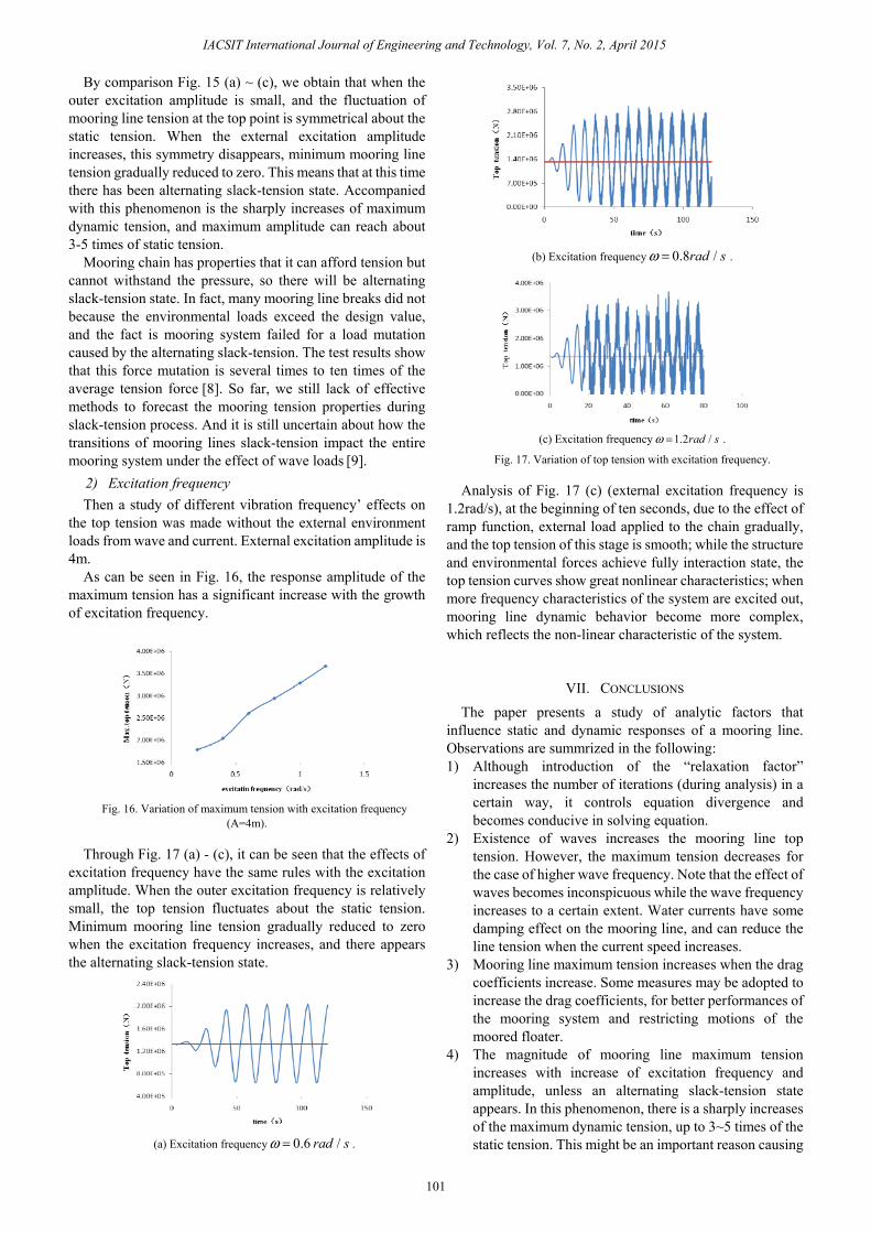
2) Excitation frequency Then a study of different vibration frequency’ effects on

the top tension was made without the external environment loads from wave and current. External excitation amplitude is 4m.

As can be seen in Fig. 16, the response amplitude of the maximum tension has a significant increase with the growth of excitation frequency.

Fig. 16. Variation of maximum tension with excitation frequency

(A=4m).

Through Fig. 17 (a) - (c), it can be seen that the effects of excitation frequency have the same rules with the excitation amplitude. When the outer excitation frequency is relatively small, the top tension fluctuates about the static tension. Minimum mooring line tension gradually reduced to zero when the excitation frequency increases, and there appears the alternating slack-tension state.

(a) Excitation frequency 0.6 /rad sω = .

(b) Excitation frequency 0.8 /rad sω = .

(c) Excitation frequency 1.2 /rad sω = .

Fig. 17. Variation of top tension with excitation frequency.

Analysis of Fig. 17 (c) (external excitation frequency is 1.2rad/s), at the beginning of ten seconds, due to the effect of ramp function, external load applied to the chain gradually, and the top tension of this stage is smooth; while the structure and environmental forces achieve fully interaction state, the top tension curves show great nonlinear characteristics; when more frequency characteristics of the system are excited out, mooring line dynamic behavior become more complex, which reflects the non-linear characteristic of the system.

VII. CONCLUSIONS The paper presents a study of analytic factors that

influence static and dynamic responses of a mooring line. Observations are summrized in the following: 1) Although introduction of the “relaxation factor”

increases the number of iterations (during analysis) in a certain way, it controls equation divergence and becomes conducive in solving equation.

2) Existence of waves increases the mooring line top tension. However, the maximum tension decreases for the case of higher wave frequency. Note that the effect of waves becomes inconspicuous while the wave frequency increases to a certain extent. Water currents have some damping effect on the mooring line, and can reduce the line tension when the current speed increases.

3) Mooring line maximum tension increases when the drag coefficients increase. Some measures may be adopted to increase the drag coefficients, for better performances of the mooring system and restricting motions of the moored floater.

4) The magnitude of mooring line maximum tension increases with increase of excitation frequency and amplitude, unless an alternating slack-tension state appears. In this phenomenon, there is a sharply increases of the maximum dynamic tension, up to 3~5 times of the static tension. This might be an important reason causing

101


the mooring system failure. Finally, the current study is based on a heavy steel chain;

further investigation is needed for a light cable in this respect.

REFERENCE [1] Y. G. Tang, “Dynamic tension of mooring system in deep sea with

finite element method,” The Ocean Engineering, vol. 27, pp. 10-15, 2009

[2] M. D. Yang and T. Bin, “Static analysis of mooring lines using nonlinear finite element method,” The Ocean Engineering, vol. 27, pp. 10-20, 2009

[3] F. F. Yu, “Research on mooring system performance of the deep-water platform,” Master thesis, Tian Jin University. 2011

[4] D. L. Garrett, “Dynamic analysis of sender rods,” OMAE, pp. 127-132, 1982.

[5] W. Nie and L. P. Sun, Computational Structure Mechanics of Ship, Harbin Engineering University Press, Harbin, China, 2003.

[6] G. R. Wang, Y. M. Yu, and Z. L. Xu, Mathematics of Scientific Computing, China Machine Press, China, 2005.

[7] X. Yuan, “Numerical research on the dynamic analysis methods of mooring lines,” Master thesis, Harbin Engineering University, 2010.

[8] K. H. Jiang, “Studies of windproof mooring water drum series,” PhD thesis, Tian Jin University, 2005.

[9] Y. G. Tang and S. X. Zhang, “Advance of study on dynamic characters of mooring systems in deep water,” The Ocean Engineering, vol. 26, pp. 120-126, 2008.

Gang Ma was born in 1984. He is an assistant professor in Deepwater Engineering and Research Center (DERC), Harbin Engineering University. His current major is on the slender rod theory of the mooring line.

Liping Sun was born in 1962. She is a professor of Harbin Engineering University. Her current research interest is in ocean engineering and technology.

Youwei Kang was born in 1987. He is a graduate in Deepwater Engineering and Research Center (DERC), Harbin Engineering University. His current major is design and analysis of offshore riser system and oil platform.

Lixin Xu was born in 1966. He is a professor of Harbin Engineering University. His current research interest is in ocean engineering and technology.

102


Effects of Different Influence Factors on Static and ...ijetch.org/vol7/774-G3011.pdfthat influence...

Documents

Transcript of Effects of Different Influence Factors on Static and ...ijetch.org/vol7/774-G3011.pdfthat influence...