EEE 303 HW # 1 SOLUTIONS - Arizona State...

EEE 303 HW # 1 SOLUTIONS

Problem 1.5Since x(t) = 0 for t < 3, we have that x(t) = U(t¡ 3)x(t).a. x(1¡ t) = x(1¡ t)U(1¡ t¡ 3) = x(1¡ t)U(¡t¡ 2) which is zero for t > ¡2.b. x(1¡ t) + x(2¡ t) = x(1¡ t)U(¡t¡ 2) + x(2¡ t)U(¡t¡ 1) which is zero for t > ¡1.c. x(1¡ t)x(2¡ t) = x(1¡ t)U(¡t¡2)x(2¡ t)U(¡t¡1) = x(1¡ t)x(2¡ t)U(¡t¡2) which is zero for t > ¡2.d. x(3t) = x(3t)U(3t¡ 3) which is zero for t < 1.e. x(t=3) = x(t=3)U(t=3¡ 3) which is zero for t < 9.

1

EEE 303 HW#2 Solutions

1.43a. Let H denote a TI system such that y = H[x] and suppose that x is periodic. That is, x(t+T)=x(t),for all t. Alternatively, in terms of the shift operator T, T-T[x] = x. Now, for y to be periodic, we should alsohave T-T [y] = y. Substituting y = H[x], we get

T-T[y] = T-TH[x]= HT-T[x] (TI system, commutes with shifts)= H[x] (x is periodic)= y

(The derivations hold in discrete time as well.)

b. The zero system (y = 0) is an easy but trivial example. A more interesting case is a low-pass filtereliminating the high frequency component of, say, x(t) = sin t + sin 10πt. (More details later.)


2.20

a. 1)0cos()()cos()()cos()(0 ∫∫∫∞

∞−

∞

∞−

∞

∞−=== dttdtttdtttu δδ

b. 0)3()2sin(5

0=+∫ dttt δπ , because δ(t+3) = 0 for t in [0,5].

c. 0)2sin(2)]2[cos()2cos()1( 1

5

5 1 =−==− =−∫ πππτπττ tdttddu , since 1 is in [-5,5].

Alternatively, using integration by parts and dttdtu )(

1 )( δ= , we have that )1()1(1 τδτ τ −−=− ddu .

Then,

[ ] 0)12sin(2cos)1()2cos()1(

)2cos()1()2cos()1(

5

5

5

5

5

5

5

5 1

=−=−+−−

=−−=−

∫

∫∫

−−

−−

πττ

πττδπδ

τπττ

τδτπττ

dd

dtt

dd

ddu

where we used the fact that δ(1-5)= δ(1+5) = 0.

2.47Let y0 = h0*x0. Then,a. 00000 2)*(2)](2[*)]([ yxhtxth == , (linearity of convolution)

b. )2()()]2([*)]([))(*()]2()([*)]([ 000000000 −−=−−=−− tytytxthtxhtxtxth ,where the first equality follows from linearity and the second from time-invariance.c. Using time-invariance, )1)])(2([*)](([)]2([*)]1([ 0000 +−=−+ ttxthtxth .

But, )2()2)])(([*)](([)]2([*)]([ 00000 −=−=− tyttxthtxth .

Hence, )1()21()]2([*)]1([ 0000 −=−+=−+ tytytxth .Alternatively, using the definition of the shift operator T and its commutativity with convolution,

010021020100 )*()(*)()]2([*)]1([ yTxhTTxThTtxth ===−+ −− .d. There is not enough information to determine the output in this case. To prove this statement we need tofind two pairs (h0,x0) that produce the same response y0 and such that their corresponding transformationsproduce different responses. For this, consider h0 (t) = U(t) (a unit step) and x0(t) = {a pulse in [0,2] withamplitude ½}. As a second pair, consider h0 (t) = y0(t), x0(t) = δ(t). For the first pair, it follows that[h0(t)]*[x0(-t)] = y0(t+2). But for the second pair, [h0(t)]*[x0(-t)] = y0(t).e. Reflections are not time-invariant operations so we need to work with the convolution integral itself.Using a transformation of the integration variable σ = −τ, we have that y0(-t) can be expressed as:

))(*()()()()()()()( 00000 txhdxthdxthdxthty =−=−+−=−−=− ∫∫∫∞

∞−

∞

∞−

∞

∞−σσσσσστττ

Notice that this is not a simple transformation of the independent variable. That is, we may not simplystate that since y0 (t) = h0(t)*x0(t), then y0 (-t) = h0(-t)*x0(-t). Even though the final relationship is true, thisstatement is wrong as an implication! The error is caused by the bad notation (h(t)*x(t) is nonsense).This error becomes apparent when we consider scaling of the independent variable. That is, using theprevious derivation it follows that y0 (at) =|a| [h0(at)]*[x0(at)] (and not h0(at)*x0(at), as one mightexpect!)f. Using the property of the unit doublet u1, that x’ = u1*x, we have that

''00011010100 )*(**)*(*)*('*'* yxhuuxuhuxhxhy =====

From the graph of y0, it follows that y(t) = ½ δ(t) – ½ δ(t-2).


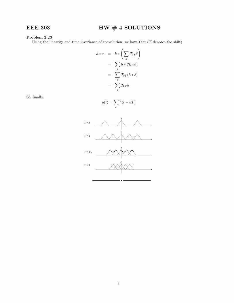
Problem 2.23Using the linearity and time invariance of convolution, we have that (T denotes the shift)

h ¤ x = h ¤ÃX

k

TkT ±!

=Xk

h ¤ (TkT ±)

=Xk

TkT (h ¤ ±)

=Xk

TkTh

So, ¯nally,

y(t) =Xk

h(t¡ kT )

T = 4

T = 2

T = 1.5

T = 1

1


3.15 The Fourier series coefficients of the output y(t), say bk are related to the Fourier series coefficients ofthe input (ak) by

bk = H(jkw0) ak

where w0 = 2π / T = 12. Since H(jw) = 0 for |w| > 100, it follows that bk = 0 for |12 k| > 100, or |k| >100/12, or |k| ≥ 9. Since it is given that x(t) = y(t), then ak = bk (uniqueness of the FS expansion), implyingthat ak must be zero for |k| ≥ 9.

EEE 303 HW Solutions

3.22.a.a Consider the derivative of the given function:

∑∞

−∞=

−−−=n

nttdtdx )12(21)( δ

The train of deltas is periodic with period 2. Its Fourier Series expansion can be found either directly(integrals of delta-times-a-function) or by using the tables and applying the shift property. We have,

∫∑−

− =−=⎭⎬⎫

⎩⎨⎧

−−=2

021

2)1()12(

00

jkwtjkw

nk

edtetntFSa δδ

where w0 = 2π/2 = π. The FS coefficients of the function 1 are 1 if k = 0 and 0 otherwise. Thus, thecoefficients of the derivative are

{ }⎩⎨⎧

−=−

==−

−

otherwiseekife

tFSb jk

jk

dtdx

k π

π 01)(

Next, the FS coefficients of x(t), say ck, are related to bk by bk = jkw0 ck. This can be solved for ck exceptfor k = 0. This can be found by applying the FS definition directly to x(t). Thus, we find

{ }⎩⎨⎧−

=== − otherwisejke

kiftxFSc jkk )/(

00)(

ππ

Notice that the direct computation of c0 here is essential. Both x(t) and x(t)+const. have the same derivativeand their FS cannot be distinguished after differentiation.

REMARK: Applying Parseval’s theorem on x(t) we find:

31

21121||

1

1

2

122

022

2 ==== ∫∑∑∑−

∞

=≠

∞

∞−

dttkk

ckk

k ππThis yields the well-known expression

61 2

12

π=∑

∞

=k k

3.22.a.b Using the same technique as in a.a, let x0 be the square wave

)()6(,0

5.0||1)( 000 txtx

otherwiset

tx =+⎩⎨⎧ <

=

whose Fourier Series coefficients are given in Table 4.2. Differentiating the given signal, we find

)5.1()5.1()( 00 −−+= txtxtdtdx

Hence, applying the linearity and time-shift properties of the Fourier Series, we get

{ } ( ) )2/sin()6/sin(2)6/sin()( 2/2/ πππ

ππ ππ k

kkjee

kktFS jkjk

dtdx =−= −

Next, using the differentiation property, we find

{ } 0),2/sin()(

)6/sin(6)/()()}({ 20 ≠=== kkkkjkwtFStxFSa dt

dxk π

ππ

while for k = 0, the FS coefficient is found by direct integration as a0 = (2+1/2+1/2)/6 = ½.


Problem 3.16bx2[n] is composed of two periodic functions, so we can apply superposition:

ys[n] = H(ej0)1 + jH(ej3¼=8)j sin(n3¼=8 + ¼=4 + argfH(ej3¼=8)g)

But H(ej0) = 0 and H(ej3¼=8) = 1, so

ys[n] = sin(n3¼=8 + ¼=4)

Alternatively, one could write the Fourier series expansion for x2 and use the ¯ltering property.

Problem 3.32The set of equations for ak is

fÁnkgn;kfakgk = fx[n]gnwhere f:gk denotes the vector or matrix indexed by k and Á = ej2¼=4. Expanding the matrices, we get2664

Á0 Á0 Á0 Á0

Á0 Á1 Á2 Á3

Á0 Á2 Á4 Á6

Á0 Á3 Á6 Á9

3775| {z }

©

2664a0a1a2a3

3775 =2664x(0)x(1)x(2)x(3)

3775 =2664

102

¡1

3775

The matrix © has a very special structure. Its columns are of the form [1; ½i; ½2i ; ½

3i ]>. Such matrices are called

Vandermonde matrices and they are nonsingular if the ½i's are distinct. In our case ½1 = Á0 = 1, ½2 = Á

1 = j,½3 = Á

2 = ¡1, ½4 = Á3 = ¡j, which are indeed distinct.In general, Vandermonde matrices are numerically ill-conditioned except when the ½i's are the n-th roots of

unity, which is our case. When this happens, the columns of the matrix are orthogonal to each other and thematrix is easy to invert. (Observe that

Pk(Á

kn1)¤Ákn2 =Pk Á

k(n2¡n1) which is 0 if n2 6= n1. This property isprecisely the reason why we can write a simple expression for the Fourier series coe±cients ak.)Regardless of any simpli¯cations, we can use Matlab (or any other numerical package) to solve the above

system of equations. Substituting the numerical values we have26641 1 1 11 j ¡1 ¡j1 ¡1 1 ¡11 ¡j ¡1 j

37752664a0a1a2a3

3775 =2664

102

¡1

3775and Matlab produces the solution a0 = 1=2, a1 = (¡1¡ j)=4, a2 = 1, a3 = (¡1 + j)=4.Needless to say, we arrive at the same result with the Fourier Series equation.

1


Problem 4.34a. From the de¯nition of the transfer function as the Fourier transform of the impulse response, we have

Y (jw)

X(jw)=

(jw) + 4

(jw)2 + 5(jw) + 6)

[(jw)2 + 5(jw) + 6]Y (jw) = [(jw) + 4]X(jw)

Taking the inverse Fourier transform of both sides, we recover the di®erential equation that describes theinput-output relationship for the system

d2

dty(t) + 5

d

dty(t) + 6y(t) =

d

dtx(t) + 4x(t)

b. We have that h(t) = F¡1fH(jw)g; using a partial fraction expansion, the roots of the denominator are¡2;¡3 and

H(jw) =A

jw + 2+

B

jw + 3

where A = [(jw + 2)H(jw)]jjw=¡2 = 2 and B = [(jw + 3)H(jw)]jjw=¡3 = ¡1. From the tables,

F¡1fH(jw)g = F¡1½

2

jw + 2

¾+ F¡1

½ ¡1jw + 3

¾= 2e¡2tU(t)¡ e¡3tU(t)

c. The response of the system to the input x(t) = e¡4tU(t) ¡ te¡4tU(t) can be found by either a directevaluation of the convolution of the impulse response with the input or by Fourier transform methods. Usingthe latter approach, we ¯nd the Fourier transform of x(t) as

X(jw) =1

jw + 4¡ 1

(jw + 4)2

Then, Y (jw) = H(jw)X(jw) so,

Y (jw) =jw + 4

(jw + 2)(jw + 3)

µ1

jw + 4¡ 1

(jw + 4)2

¶=

1

(jw + 2)(jw + 3)¡ 1

(jw + 2)(jw + 3)(jw + 4)

=1

(jw + 2)+

¡1(jw + 3)

¡ 1=2

(jw + 2)¡ ¡1(jw + 3)

¡ 1=2

(jw + 4)

=1=2

(jw + 2)¡ 1=2

(jw + 4)

It is now straightforward to evaluate the time response:

y(t) = F¡1fY (jw)g = 1

2

£e¡2tU(t)¡ e¡4tU(t)¤

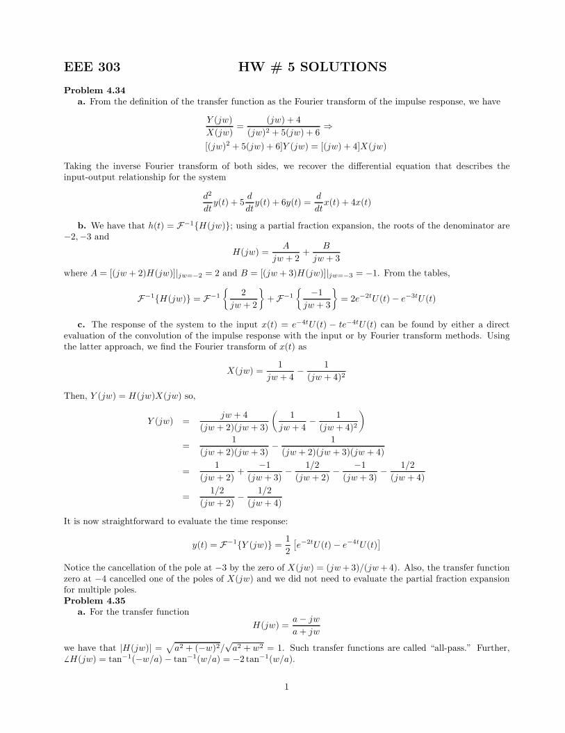
Notice the cancellation of the pole at ¡3 by the zero of X(jw) = (jw+3)=(jw+4). Also, the transfer functionzero at ¡4 cancelled one of the poles of X(jw) and we did not need to evaluate the partial fraction expansionfor multiple poles.Problem 4.35a. For the transfer function

H(jw) =a¡ jwa+ jw

we have that jH(jw)j = pa2 + (¡w)2=pa2 + w2 = 1. Such transfer functions are called \all-pass." Further,

6H(jw) = tan¡1(¡w=a)¡ tan¡1(w=a) = ¡2 tan¡1(w=a).

1

b. The impulse response of the system is the inverse Fourier transform of its transfer function:

h(t) = F¡1 fH(jw)g = F¡1½a+ a¡ a¡ jw

a+ jw

¾= F¡1

½2a

a+ jw¡ 1¾= 2ae¡atU(t)¡ ±(t)

c. The response of the system to the input

x(t) = cos(t=p3) + cos(t) + cos(

p3t)

can be evaluated through Fourier transforms. X(jw) will contain 6 impulses and so will the productX(jw)H(jw).Then the inverse transform will contain 6 complex exponentials, but the simpli¯cation of that formula is quitetedious.Alternatively, using the sinusoid response formula and for a = 1,1

y(t) = cos(t=p3¡ 2 tan¡1(1=

p3)) + cos(t¡ 2 tan¡1(1)) + cos(

p3t¡ 2 tan¡1(

p3))

= cos(t=p3¡ ¼=3) + cos(t¡ ¼=2) + cos(

p3t¡ 2¼=3)

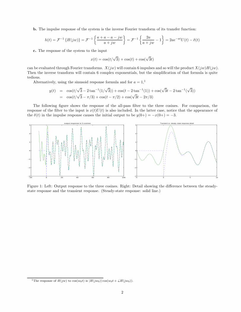
The following ¯gure shows the response of the all-pass ¯lter to the three cosines. For comparison, theresponse of the ¯lter to the input is x(t)U(t) is also included. In the latter case, notice that the appearance ofthe ±(t) in the impulse response causes the initial output to be y(0+) = ¡x(0+) = ¡3.

−20 0 20 40 60 80 100−3

−2

−1

0

1

2

3output response to 3 cosines

−5 0 5 10−3

−2

−1

0

1

2

3Transient vs. steady−state response detail

Figure 1: Left: Output response to the three cosines. Right: Detail showing the di®erence between the steady-state response and the transient response. (Steady-state response: solid line.)

1The response of H(jw) to cos(w0t) is jH(jw0)j cos(w0t+6H(jw0)).

2


Problem 5.10Let A =

P10 n

12n and de¯ne the sequence x[n] =

12nu[n]. Then X(e

jw) = 11¡e¡jw=2 . The transform of the

sequence nx[n] is j dX(ejw)

dw = e¡jw=2(1¡e¡jw=2)2 . Then, A = Ffnx[n]gjej0 =

1=2(1¡1=2)2 = 2

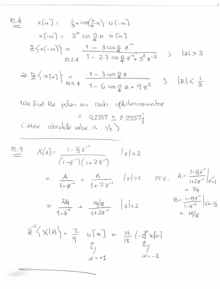
Problem 5.19By inspection, the transfer function is

H(z) =1

1¡ 16z¡1 ¡ 1

6z¡2

where z = ejw.The poles (roots of denominator) are z = 1=2 and ¡1=3. Taking the Partial Fraction Expansion we have

H(z) =1

(1¡ 12z¡1)(1 + 1

3z¡1)

=35

1¡ 12z¡1 +

25

1 + 13z¡1

Using the tables to ¯nd the inverse Fourier, we get

h[n] =3

5

µ1

2

¶nu[n] +

2

5

µ¡13

¶nu[n]

Note: The impulse response can also be computed directly from the recursion. First, since the system islinear, its response to the zero input sequence is zero. Furthermore since it is causal, then its response to ±[n]must be identical to the zero-input response up to the index n = 0. So, y[n] = 0, for n < 0. Then,

y[0] = 0 + 0 + x[0] = 1

y[1] = 1=6¡ 0 + 0 = 1=6y[2] = (1=6)(1=6) + 1=6 + 0 = 7=36

...

which is the same as the previous analytical computations.

1


Problem 6.9The ¯lter is stable so the steady-state response is well-de¯ned. The steady-state part of the step is the

constant function 1. The ¯lter transfer function is H(jw) = 2jw+5 which at w = 0 is 2/5. Therefore, the

steady-state part of the step response is the constant function (2/5)(1) = 2/5, which is also the ¯nal value ofys(t); t!1.The step response is Ys(s) =

2s+5

1s. Taking the inverse Laplace via partial fraction expansion we ¯nd:

ys(t) = L¡1½

2

s+ 5

1

s

¾= L¡1

½2=5

s+¡2=5s+ 5

¾=2

5u(t)¡ 2

5e¡5tu(t) =

2

5(1¡ e¡5t)u(t)

The same result is obtained by using the Fourier transform, but notice the di®erence in the transform of thestep function:

Ys(jw) =2

jw + 5

µ1

jw+ ¼±(w)

¶=2

5¼±(w) +

2

jw + 5

1

jw

ys(t) = F¡1 fYs(jw)g = F¡1½2

5¼±(w) +

2

jw + 5

1

jw

¾= F¡1

½2

5¼±(w) +

2=5

jw+¡2=5jw + 5

¾= F¡1

½2

5

µ1

jw+ ¼±(w)

¶+¡2=5jw + 5

¾=2

5u(t)¡ 2

5e¡5tu(t)

As t ! 1, this expression yields ys(1) = 2=5, as found in the ¯rst part. Then, the time t0 at whichys(t0) = ys(1)(1¡ e¡2) is t0 = 2=5.

Problem 6.12The transfer function of the cascade connection is H(jw) = H1(jw)H2(jw). Hence, H2(jw) =

H(jw)H1(jw)

.

Taking the magnitude and log of both sides,

log10 jH2(jw)j = log10 jH(jw)j ¡ log10 jH1(jw)j ) jH2(jw)jdB = jH(jw)jdB ¡ jH1(jw)jdBThus the straight-line approximation of jH2(jw)jdB is described as follows:for w < 1: constant with magnitude (-20)-(6) = -26 dB;

for < 1w < 8: straight line with slope (0)-(20) = -20 dB/dec;

for 8 < w < 40: straight line with slope (-40)-(0) = -40 dB/dec;

for 40 < w: straight line with slope (-40)-(-20) = -20 dB/dec;

1


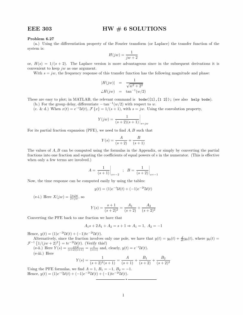
Problem 6.27(a.) Using the di®erentiation property of the Fourier transform (or Laplace) the transfer function of the

system is:

H(jw) =1

jw + 2

or, H(s) = 1=(s + 2). The Laplace version is more advantageous since in the subsequent derivations it isconvenient to keep jw as one argument.With s = jw, the frequency response of this transfer function has the following magnitude and phase:

jH(jw)j =1p

w2 + 22

6H(jw) = tan¡1(w=2)

These are easy to plot; in MATLAB, the relevant command is bode([1],[1 2]); (see also help bode).(b.) For the group delay, di®erentiate ¡ tan¡1(w=2) with respect to w.(c. & d.) When x(t) = e¡tU(t), F fxg = 1=(s+ 1), with s = jw. Using the convolution property,

Y (jw) =1

(s+ 2)(s+ 1)

¯̄̄̄s=jw

For its partial fraction expansion (PFE), we need to ¯nd A;B such that

Y (s) =A

(s+ 2)+

B

(s+ 1)

The values of A;B can be computed using the formulas in the Appendix, or simply by converting the partialfractions into one fraction and equating the coe±cients of equal powers of s in the numerator. (This is e®ectivewhen only a few terms are involved.)

A =1

(s+ 1)

¯̄̄̄s=¡2

; B =1

(s+ 2)

¯̄̄̄s=¡1

Now, the time response can be computed easily by using the tables:

y(t) = (1)e¡tU(t) + (¡1)e¡2tU(t)(e-i.) Here X(jw) = 1+jw

2+jw , so

Y (s) =s+ 1

(s+ 2)2=

A1(s+ 2)

+A2

(s+ 2)2

Converting the PFE back to one fraction we have that

A1s+ 2A1 +A2 = s+ 1) A1 = 1; A2 = ¡1Hence, y(t) = (1)e¡2tU(t) + (¡1)te¡2tU(t).Alternatively, since the fraction involves only one pole, we have that y(t) = y0(t) +

ddty0(t), where y0(t) =

F¡1 ©1=(jw + 2)2ª = te¡2tU(t). (Verify this!)(e-ii.) Here Y (s) = s+2

(s+2)(s+1)= 1

(s+1)and, clearly, y(t) = e¡tU(t).

(e-iii.) Here

Y (s) =1

(s+ 2)2(s+ 1)=

A

(s+ 1)+

B1(s+ 2)

+B2

(s+ 2)2

Using the PFE formulas, we ¯nd A = 1, B1 = ¡1, B2 = ¡1.Hence, y(t) = (1)e¡tU(t) + (¡1)e¡2tU(t) + (¡1)te¡2tU(t).

1


Problem 7.4The Nyquist rate of x(t) is w0, so x(t) is bandlimited in (¡w0=2; w0=2). In other words, the maximum

frequency where x(t) has energy is wM = w0=2.1. F fx(t¡ 1)g = e¡jwF fx(t)g is also bandlimited in (¡wM ; wM ). Hence, F fx(t¡ 1) + x(t)g is bandlim-

ited in (¡wM ; wM ), and the Nyquist rate of x(t¡ 1) + x(t) is 2wm = w0.2. F ©dx

dt

ª= jwF fx(t)g which is again bandlimited in (¡wM ; wM ) and, hence, the Nyquist rate of dx=dt

is w0.Notice that this result hinges on the assumption that X(jw) is zero for jwj > wM . This can be deceptive in

a practical situation where the Nyquist rate is de¯ned in terms of the signal \bandwidth," i.e., the frequencybeyond which the energy content of the signal is small. In such a case, di®erentiation of the signal will increasethe magnitude (and energy) of the signal at high frequencies and will change the e®ective Nyquist rate.3. Let y(t) = x2(t). Then F fyg = 1

2¼F fxg ¤ F fxg. Since F fxg is bandlimited in (¡wM ; wM ), we have

that F fyg is bandlimited in (¡2wM ; 2wM ); hence the Nyquist rate of y(t) is 2w0.4. Let y(t) = x(t) cos(w0t). Then F fyg = 1

2¼F fxgF fcosw0tg = 1

2[X(j(w¡w0)) +X(j(w+w0))]. Hence,

F fyg is bandlimited in (¡w0 ¡ wM ; w0 + wM ) = (¡3wM ;¡3wM ) and the Nyquist rate of y(t) is 6wM = 3w0.Problem 7.22Let x1(t) be bandlimited in (¡1000¼; 1000¼) and x2(t) be bandlimited in (¡2000¼; 2000¼).a. Let y(t) = (x1 ¤ x2)(t). Then F fyg = F fx1gF fx2g which is bandlimited in the intersection of the

two frequency intervals, that is (¡1000¼; 1000¼). Hence the Nyquist rate of y(t) is 2000¼ and the maximumsampling time to allow perfect reconstruction is T = 2¼=(2000¼) = 1=1000.b. Let y(t) = 2¼x1(t)x2(t). Then F fyg = F fx1g ¤ F fx2g which is bandlimited in the frequency interval

(¡1000¼¡ 2000¼; 1000¼+2000¼). Hence the Nyquist rate of y(t) is 6000¼ and the maximum sampling time toallow perfect reconstruction is T = 2¼=(6000¼) = 1=3000.

1

EEE 3 03 HW # 7 SOLUT I ONS

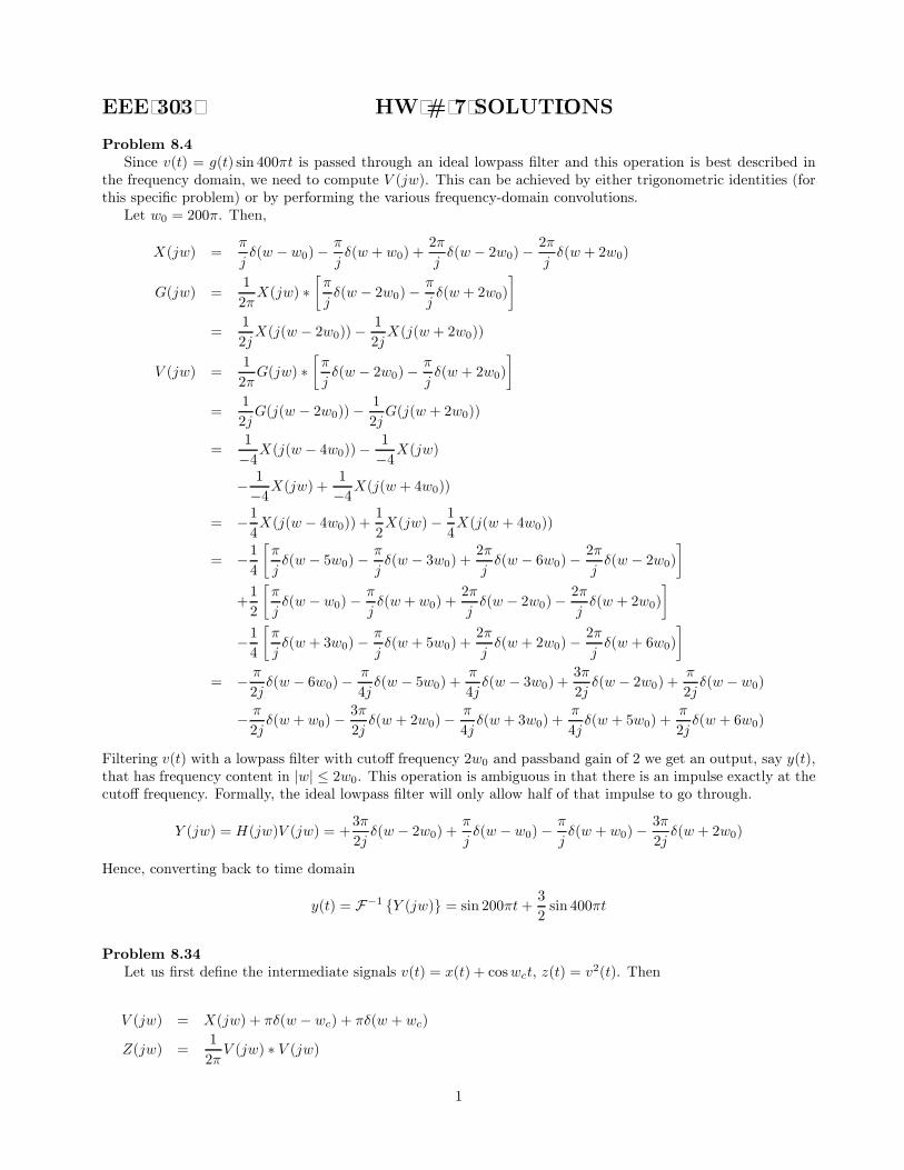
Problem 8.4Since v(t) = g(t) sin 400¼t is passed through an ideal lowpass ¯lter and this operation is best described in

the frequency domain, we need to compute V (jw). This can be achieved by either trigonometric identities (forthis speci¯c problem) or by performing the various frequency-domain convolutions.Let w0 = 200¼. Then,

X(jw) =¼

j±(w ¡ w0)¡ ¼

j±(w + w0) +

2¼

j±(w ¡ 2w0)¡ 2¼

j±(w + 2w0)

G(jw) =1

2¼X(jw) ¤

∙¼

j±(w ¡ 2w0)¡ ¼

j±(w + 2w0)

¸=

1

2jX(j(w ¡ 2w0))¡ 1

2jX(j(w + 2w0))

V (jw) =1

2¼G(jw) ¤

∙¼

j±(w ¡ 2w0)¡ ¼

j±(w + 2w0)

¸=

1

2jG(j(w ¡ 2w0))¡ 1

2jG(j(w + 2w0))

=1

¡4X(j(w ¡ 4w0))¡1

¡4X(jw)

¡ 1

¡4X(jw) +1

¡4X(j(w + 4w0))

= ¡14X(j(w ¡ 4w0)) + 1

2X(jw)¡ 1

4X(j(w + 4w0))

= ¡14

∙¼

j±(w ¡ 5w0)¡ ¼

j±(w ¡ 3w0) + 2¼

j±(w ¡ 6w0)¡ 2¼

j±(w ¡ 2w0)

¸+1

2

∙¼

j±(w ¡ w0)¡ ¼

j±(w + w0) +

2¼

j±(w ¡ 2w0)¡ 2¼

j±(w + 2w0)

¸¡14

∙¼

j±(w + 3w0)¡ ¼

j±(w + 5w0) +

2¼

j±(w + 2w0)¡ 2¼

j±(w + 6w0)

¸= ¡ ¼

2j±(w ¡ 6w0)¡ ¼

4j±(w ¡ 5w0) + ¼

4j±(w ¡ 3w0) + 3¼

2j±(w ¡ 2w0) + ¼

2j±(w ¡ w0)

¡ ¼2j±(w + w0)¡ 3¼

2j±(w + 2w0)¡ ¼

4j±(w + 3w0) +

¼

4j±(w + 5w0) +

¼

2j±(w + 6w0)

Filtering v(t) with a lowpass ¯lter with cuto® frequency 2w0 and passband gain of 2 we get an output, say y(t),that has frequency content in jwj ∙ 2w0. This operation is ambiguous in that there is an impulse exactly at thecuto® frequency. Formally, the ideal lowpass ¯lter will only allow half of that impulse to go through.

Y (jw) = H(jw)V (jw) = +3¼

2j±(w ¡ 2w0) + ¼

j±(w ¡ w0)¡ ¼

j±(w + w0)¡ 3¼

2j±(w + 2w0)

Hence, converting back to time domain

y(t) = F¡1 fY (jw)g = sin 200¼t+ 32sin 400¼t

Problem 8.34Let us ¯rst de¯ne the intermediate signals v(t) = x(t) + coswct, z(t) = v

2(t). Then

V (jw) = X(jw) + ¼±(w ¡ wc) + ¼±(w + wc)Z(jw) =

1

2¼V (jw) ¤ V (jw)

1

=1

2X(j(w ¡ wc)) + ¼

2±(w ¡ 2wc) + ¼

2±(w)

+1

2X(j(w + wc)) +

¼

2±(w) +

¼

2±(w + 2wc)

+1

2X(j(w ¡ wc)) + 1

2X(j(w + wc)) +

1

2¼X(jw) ¤X(jw)

= X(j(w ¡ wc)) +X(j(w + wc)) + ¼2±(w ¡ 2wc) + ¼

2±(w + 2wc) + ¼±(w) +

1

2¼X(jw) ¤X(jw)

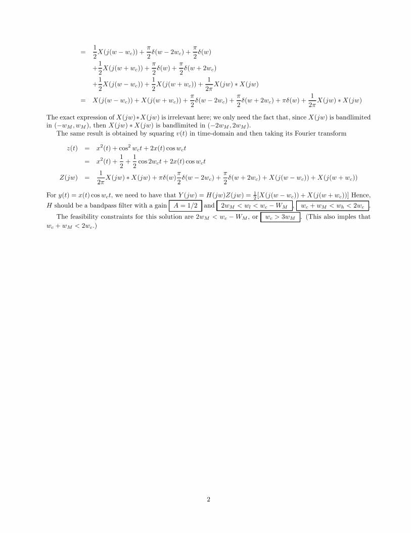
The exact expression of X(jw)¤X(jw) is irrelevant here; we only need the fact that, since X(jw) is bandlimitedin (¡wM ; wM ), then X(jw) ¤X(jw) is bandlimited in (¡2wM ; 2wM ).The same result is obtained by squaring v(t) in time-domain and then taking its Fourier transform

z(t) = x2(t) + cos2 wct+ 2x(t) coswct

= x2(t) +1

2+1

2cos 2wct+ 2x(t) coswct

Z(jw) =1

2¼X(jw) ¤X(jw) + ¼±(w)¼

2±(w ¡ 2wc) + ¼

2±(w + 2wc) +X(j(w ¡ wc)) +X(j(w + wc))

For y(t) = x(t) coswct, we need to have that Y (jw) = H(jw)Z(jw) =12[X(j(w ¡wc)) +X(j(w +wc))] Hence,

H should be a bandpass ¯lter with a gain A = 1=2 and 2wM < wl < wc ¡WM , wc + wM < wh < 2wc .

The feasibility constraints for this solution are 2wM < wc ¡WM , or wc > 3wM . (This also imples that

wc + wM < 2wc.)

2

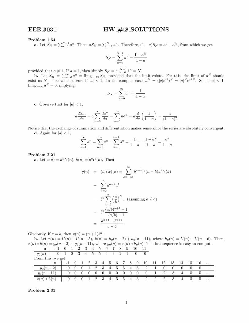
EEE 3 03 HW # 8 SOLUT I ONS

Problem 1.54a. Let SN =

PN¡1n=0 a

n. Then, aSN =PN

n=1 an. Therefore, (1¡ a)SN = a0 ¡ aN , from which we get

SN =

N¡1Xn=0

an =1¡ aN1¡ a

provided that a6= 1. If a = 1, then simply SN =PN¡1

n=0 1n = N .

b. Let S1 =P1

n=0 an = limN!1 SN , provided that the limit exists. For this, the limit of aN should

exist as N ! 1 which occurs if jaj < 1. In the complex case, aN = (jajejµ)N = jajNejµN . So, if jaj < 1,limN!1 aN = 0, implying

S1 =

1Xn=0

an =1

1¡ ac. Observe that for jaj < 1,

adS1da

= a

1Xn=0

dan

da=

1Xn=0

nan = ad

da

µ1

1¡ a¶=

1

(1¡ a)2

Notice that the exchange of summation and di®erentiation makes sense since the series are absolutely convergent.d. Again for jaj < 1,

1Xn=k

an =

1Xn=0

an ¡k¡1Xn=0

an =1

1¡ a ¡1¡ ak1¡ a =

ak

1¡ a

Problem 2.21a. Let x(n) = anU(n), h(n) = bnU(n). Then

y(n) = (h ¤ x)(n) =1X

k=¡1bn¡kU(n¡ k)akU(k)

=

nXk=0

bn¡kak

= bnnXk=0

³ab

´k; (assuming b6= a)

= bn(a=b)n+1 ¡ 1(a=b)¡ 1

=an+1 ¡ bn+1

a¡ bObviously, if a = b, then y(n) = (n+ 1)bn.b. Let x(n) = U(n) ¡ U(n ¡ 5), h(n) = h0(n ¡ 2) + h0(n ¡ 11), where h0(n) = U(n) ¡ U(n ¡ 6). Then,

x(n) ¤ h(n) = y0(n¡ 2) + y0(n¡ 11), where y0(n) = x(n) ¤ h0(n). The last sequence is easy to compute:n -1 0 1 2 3 4 5 6 7 8 9 10 11

y0(n) 0 1 2 3 4 5 5 4 3 2 1 0 0From this, we get

n -1 0 1 2 3 4 5 6 7 8 9 10 11 12 13 14 15 16 . . .y0(n¡ 2) 0 0 0 1 2 3 4 5 5 4 3 2 1 0 0 0 0 0 . . .y0(n¡ 11) 0 0 0 0 0 0 0 0 0 0 0 0 1 2 3 4 5 5 . . .

x(n) ¤ h(n) 0 0 0 1 2 3 4 5 5 4 3 2 2 2 3 4 5 5 . . .

Problem 2.31

1

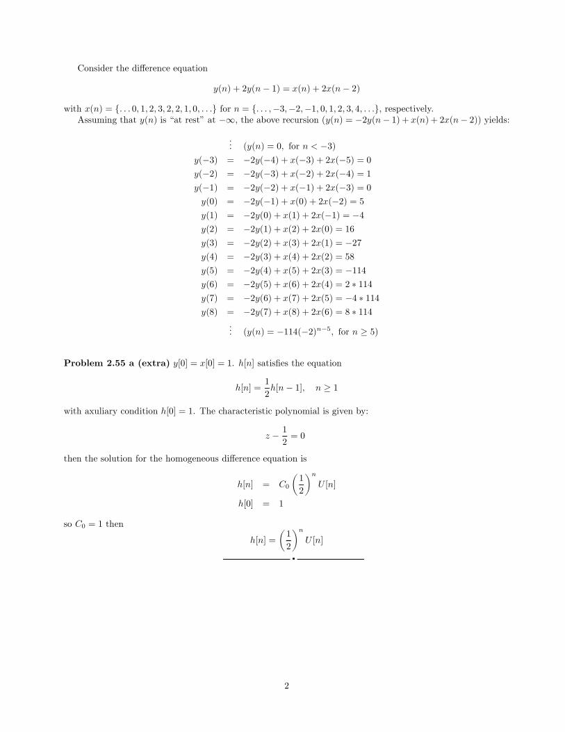
Consider the di®erence equation

y(n) + 2y(n¡ 1) = x(n) + 2x(n¡ 2)

with x(n) = f: : : 0; 1; 2; 3; 2; 2; 1; 0; : : :g for n = f: : : ;¡3;¡2;¡1; 0; 1; 2; 3; 4; : : :g, respectively.Assuming that y(n) is \at rest" at ¡1, the above recursion (y(n) = ¡2y(n¡ 1) + x(n) + 2x(n¡ 2)) yields:

... (y(n) = 0; for n < ¡3)y(¡3) = ¡2y(¡4) + x(¡3) + 2x(¡5) = 0y(¡2) = ¡2y(¡3) + x(¡2) + 2x(¡4) = 1y(¡1) = ¡2y(¡2) + x(¡1) + 2x(¡3) = 0y(0) = ¡2y(¡1) + x(0) + 2x(¡2) = 5y(1) = ¡2y(0) + x(1) + 2x(¡1) = ¡4y(2) = ¡2y(1) + x(2) + 2x(0) = 16y(3) = ¡2y(2) + x(3) + 2x(1) = ¡27y(4) = ¡2y(3) + x(4) + 2x(2) = 58y(5) = ¡2y(4) + x(5) + 2x(3) = ¡114y(6) = ¡2y(5) + x(6) + 2x(4) = 2 ¤ 114y(7) = ¡2y(6) + x(7) + 2x(5) = ¡4 ¤ 114y(8) = ¡2y(7) + x(8) + 2x(6) = 8 ¤ 114

... (y(n) = ¡114(¡2)n¡5; for n ¸ 5)

Problem 2.55 a (extra) y[0] = x[0] = 1. h[n] satis¯es the equation

h[n] =1

2h[n¡ 1]; n ¸ 1

with axuliary condition h[0] = 1. The characteristic polynomial is given by:

z ¡ 12= 0

then the solution for the homogeneous di®erence equation is

h[n] = C0

µ1

2

¶nU [n]

h[0] = 1

so C0 = 1 then

h[n] =

µ1

2

¶nU [n]

2

EEE 303 HW # 1 SOLUTIONS - Arizona State...

Documents

Transcript of EEE 303 HW # 1 SOLUTIONS - Arizona State...