EEE 103 - Load Flow Analysis
107
4 Electrical and Electronics Engineering Institute University of the Philippines RDDELMUNDO EEE 103 AY2010-11 S2 EEE 103 – Introduction to Power Systems Power Flow Through Short Transmission Lines Let us consider a short transmission line. The single-phase equivalent circuit is shown below: • • • • + - V s = |V s | ∠α V R = |V R | ∠0 + - I s I R Z = (r + jx L )L = |Z| ∠θ I S = I R = I V S = ZI + V R
-
Upload
vanessa-tan -
Category
Documents
-
view
270 -
download
13
Transcript of EEE 103 - Load Flow Analysis

4 Electrical and Electronics Engineering Institute University of the Philippines
RDDELMUNDO EEE 103 AY2010-11 S2
EEE 103 – Introduction to Power Systems
Power Flow Through Short Transmission Lines
Let us consider a short transmission line. The single-phase equivalent circuit is shown below:
• •
• • +
-
Vs = |Vs| ∠α VR = |VR| ∠0
+
-
Is IR
Z = (r + jxL )L = |Z| ∠θ
IS = IR = I VS = ZI + VR
5 Electrical and Electronics Engineering Institute University of the Philippines
RDDELMUNDO EEE 103 AY2010-11 S2
EEE 103 – Introduction to Power Systems
We calculate for the current I and its conjugate I* : ( ) ( )
( )( ) ( )
( )
0
0
S R
S R
V VI
Z
V VI
Z
α
θ
α
θ∗ −
−
∠ − ∠=
∠
∠ − ∠=
∠
v
v
We calculate the single-phase complex power at the sending and receiving ends:
( )
( 0)S S
R R
S V IS V I
α ∗
∗
= ∠ ⋅
= ∠ ⋅
v vv v
The direction of power flow will be inherent in the direction of the current I, i.e., SS is the supplied power when positive, and SR is the load power when positive.
6 Electrical and Electronics Engineering Institute University of the Philippines
RDDELMUNDO EEE 103 AY2010-11 S2
EEE 103 – Introduction to Power Systems
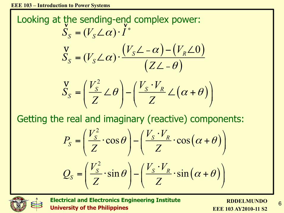
Looking at the sending-end complex power:
( )
( )
2
2
cos cos
sin sin
S S RS
S S RS
V V VPZ Z
V V VQZ Z
θ α θ
θ α θ
# $ ⋅# $= ⋅ − ⋅ +' ( ' () *) *
# $ ⋅# $= ⋅ − ⋅ +' ( ' () *) *
Getting the real and imaginary (reactive) components:
( ) ( )( )
( )2
( )0
( )
S S
S RS S
S S RS
S V IV V
S VZ
V V VSZ Z
α
αα
θ
θ α θ
∗
−
−
= ∠ ⋅
∠ − ∠= ∠ ⋅
∠
' ( ⋅' (= ∠ − ∠ +) * ) *+ ,+ ,
v v
v
v
7 Electrical and Electronics Engineering Institute University of the Philippines
RDDELMUNDO EEE 103 AY2010-11 S2
EEE 103 – Introduction to Power Systems
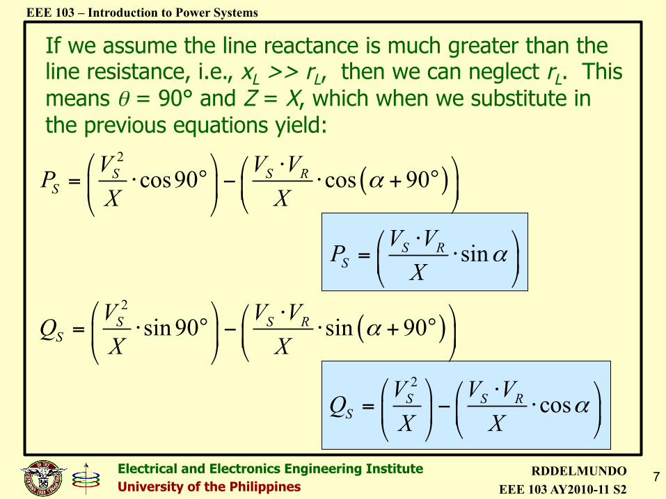
If we assume the line reactance is much greater than the line resistance, i.e., xL >> rL, then we can neglect rL. This means θ = 90° and Z = X, which when we substitute in the previous equations yield:
( )
( )
2
2
2
cos90 cos 90
sin
sin 90 sin 90
cos
S S RS
S RS
S S RS
S S RS
V V VPX X
V VPX
V V VQX X
V V VQX X
α
α
α
α
" # ⋅" #= ⋅ ° − ⋅ + °& ' & '( )( )
⋅" #= ⋅& '( )
" # ⋅" #= ⋅ ° − ⋅ + °& ' & '( )( )
" # ⋅" #= − ⋅& ' & '
( )( )
8 Electrical and Electronics Engineering Institute University of the Philippines
RDDELMUNDO EEE 103 AY2010-11 S2
EEE 103 – Introduction to Power Systems
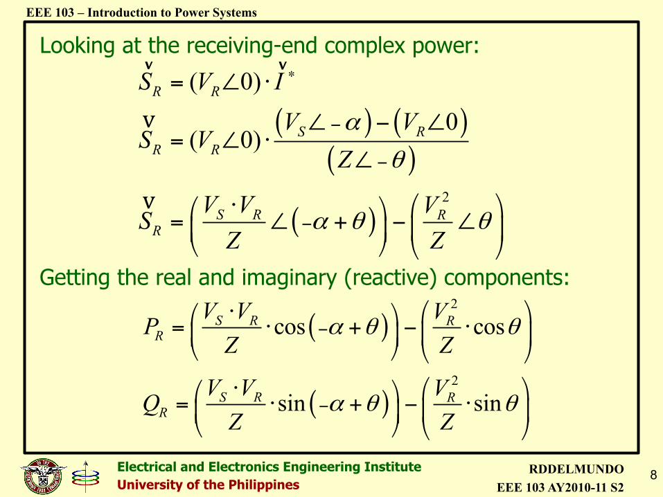
Looking at the receiving-end complex power:
( )
( )
2
2
cos cos
sin sin
S R RR
S R RR
V V VPZ Z
V V VQZ Z
α θ θ
α θ θ
−
−
$ %⋅$ %= ⋅ + − ⋅' (' () * ) *
$ %⋅$ %= ⋅ + − ⋅' (' () * ) *
Getting the real and imaginary (reactive) components:
( ) ( )( )
( )2
( 0)0
( 0)
R R
S RR R
S R RR
S V IV V
S VZ
V V VSZ Z
α
θ
α θ θ
∗
−
−
−
= ∠ ⋅
∠ − ∠= ∠ ⋅
∠
' (⋅' (= ∠ + − ∠) *) *+ , + ,
v v
v
v
9 Electrical and Electronics Engineering Institute University of the Philippines
RDDELMUNDO EEE 103 AY2010-11 S2
EEE 103 – Introduction to Power Systems
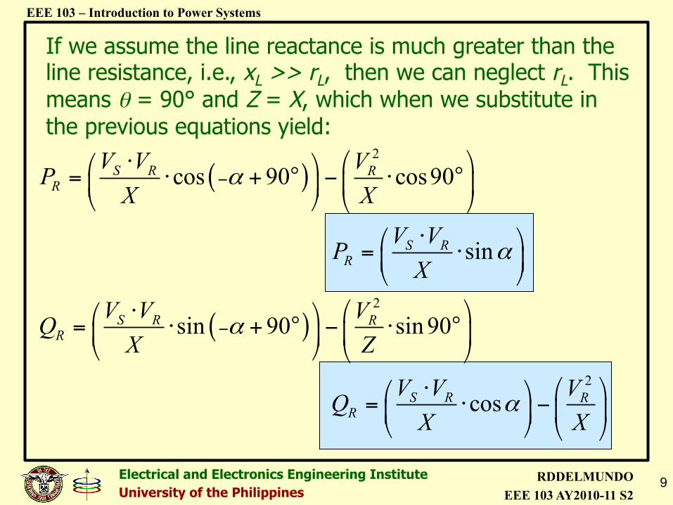
If we assume the line reactance is much greater than the line resistance, i.e., xL >> rL, then we can neglect rL. This means θ = 90° and Z = X, which when we substitute in the previous equations yield:
( )
( )
2
2
2
cos 90 cos90
sin
sin 90 sin90
cos
S R RR
S RR
S R RR
S R RR
V V VPX X
V VPX
V V VQX Z
V V VQX X
α
α
α
α
−
−
# $⋅# $= ⋅ + ° − ⋅ °& '& '( ) ( )
⋅# $= ⋅& '( )
# $⋅# $= ⋅ + ° − ⋅ °& '& '( ) ( )
# $⋅# $= ⋅ − & '& '( ) ( )
10 Electrical and Electronics Engineering Institute University of the Philippines
RDDELMUNDO EEE 103 AY2010-11 S2
EEE 103 – Introduction to Power Systems
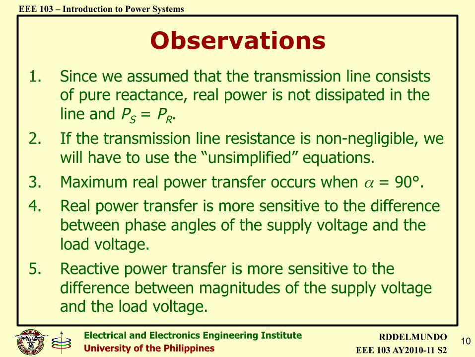
Observations 1. Since we assumed that the transmission line consists
of pure reactance, real power is not dissipated in the line and PS = PR.
2. If the transmission line resistance is non-negligible, we will have to use the “unsimplified” equations.
3. Maximum real power transfer occurs when α = 90°. 4. Real power transfer is more sensitive to the difference
between phase angles of the supply voltage and the load voltage.
5. Reactive power transfer is more sensitive to the difference between magnitudes of the supply voltage and the load voltage.
12 Electrical and Electronics Engineering Institute University of the Philippines
RDDELMUNDO EEE 103 AY2010-11 S2
EEE 103 – Introduction to Power Systems
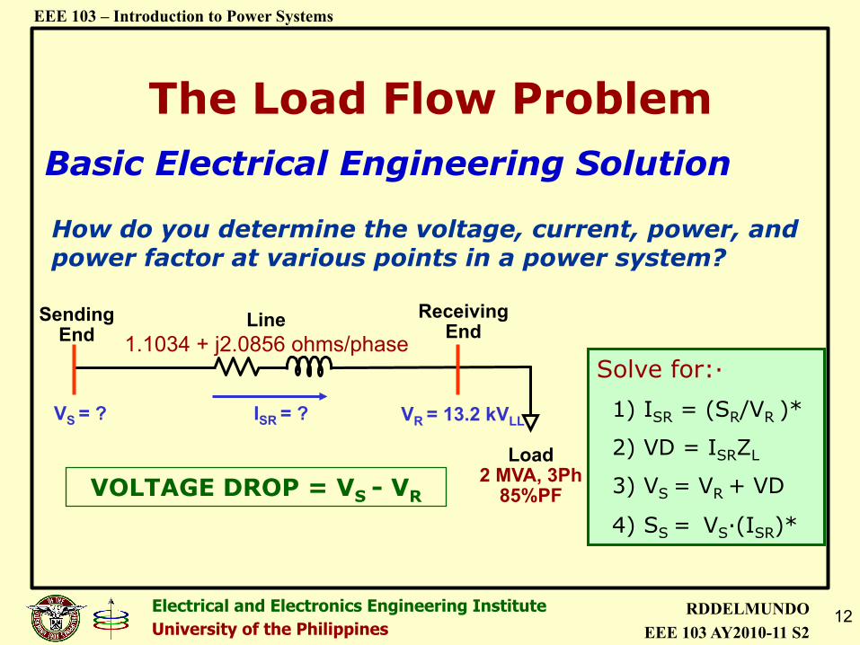
The Load Flow Problem
How do you determine the voltage, current, power, and power factor at various points in a power system?
Sending End
Receiving End
VS = ?
Load 2 MVA, 3Ph
85%PF
VR = 13.2 kVLL
Line 1.1034 + j2.0856 ohms/phase
ISR = ?
VOLTAGE DROP = VS - VR
Solve for:· 1) ISR = (SR/VR )*
2) VD = ISRZL
3) VS = VR + VD
4) SS = VS·(ISR)*
Basic Electrical Engineering Solution
13 Electrical and Electronics Engineering Institute University of the Philippines
RDDELMUNDO EEE 103 AY2010-11 S2
EEE 103 – Introduction to Power Systems
The Load Flow Problem Sending
End Receiving
End
VS = ?
Load 2 MVA, 3Ph
85%PF
VR = 13.2 kVLL
Line 1.1034 + j2.0856 ohms/phase
ISR = ?
Solve for: 1) ISR = (SR/VR )*
2) VD = ISRZL
3) VS = VR + VD
4) SS = VS·(ISR)*
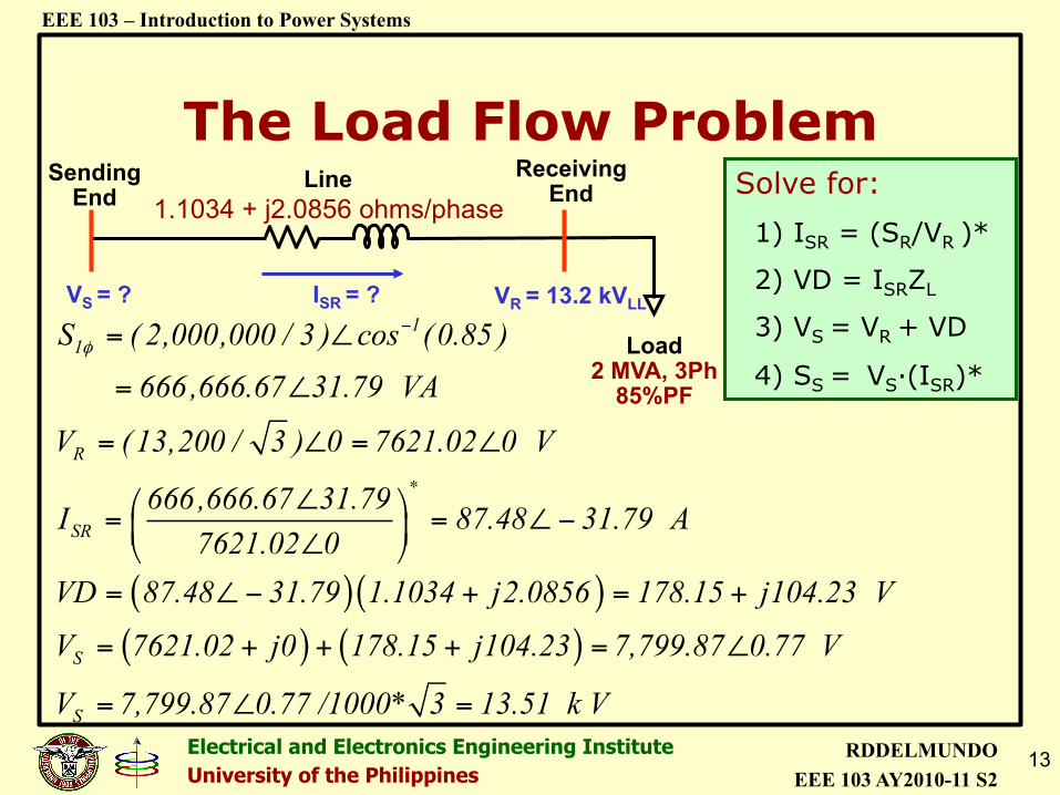
( )( )( )
11
R
SR
S
S ( 2,000,000 / 3 ) cos (0.85 )
666,666.67 31.79 VA
V (13,200 / 3 ) 0 7621.02 0 V
666,666.67 31.79I 87.48 31.79 A
7621.02 0VD 87.48 31.79 1.1034 j2.0856 178.15 j104.23 V
V 7621.02 j0 178
φ−
∗
= ∠
= ∠
= ∠ = ∠
∠% &= = ∠−' (∠) *
= ∠− + = +
= + + ( )
S
.15 j104.23 7,799.87 0.77 V
V 7,799.87 0.77 /1000* 3 13.51 k V
+ = ∠
= ∠ =
14 Electrical and Electronics Engineering Institute University of the Philippines
RDDELMUNDO EEE 103 AY2010-11 S2
EEE 103 – Introduction to Power Systems
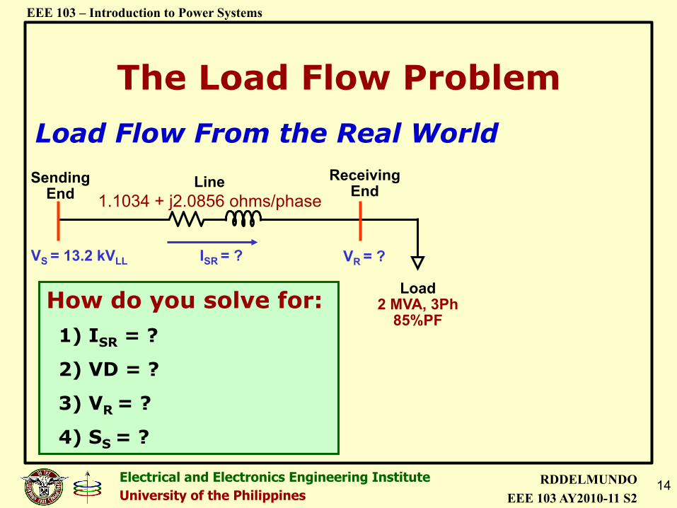
The Load Flow Problem
Sending End
Receiving End
VS = 13.2 kVLL
Load 2 MVA, 3Ph
85%PF
VR = ?
Load Flow From the Real World Line
1.1034 + j2.0856 ohms/phase
ISR = ?
How do you solve for: 1) ISR = ?
2) VD = ?
3) VR = ?
4) SS = ?
15 Electrical and Electronics Engineering Institute University of the Philippines
RDDELMUNDO EEE 103 AY2010-11 S2
EEE 103 – Introduction to Power Systems
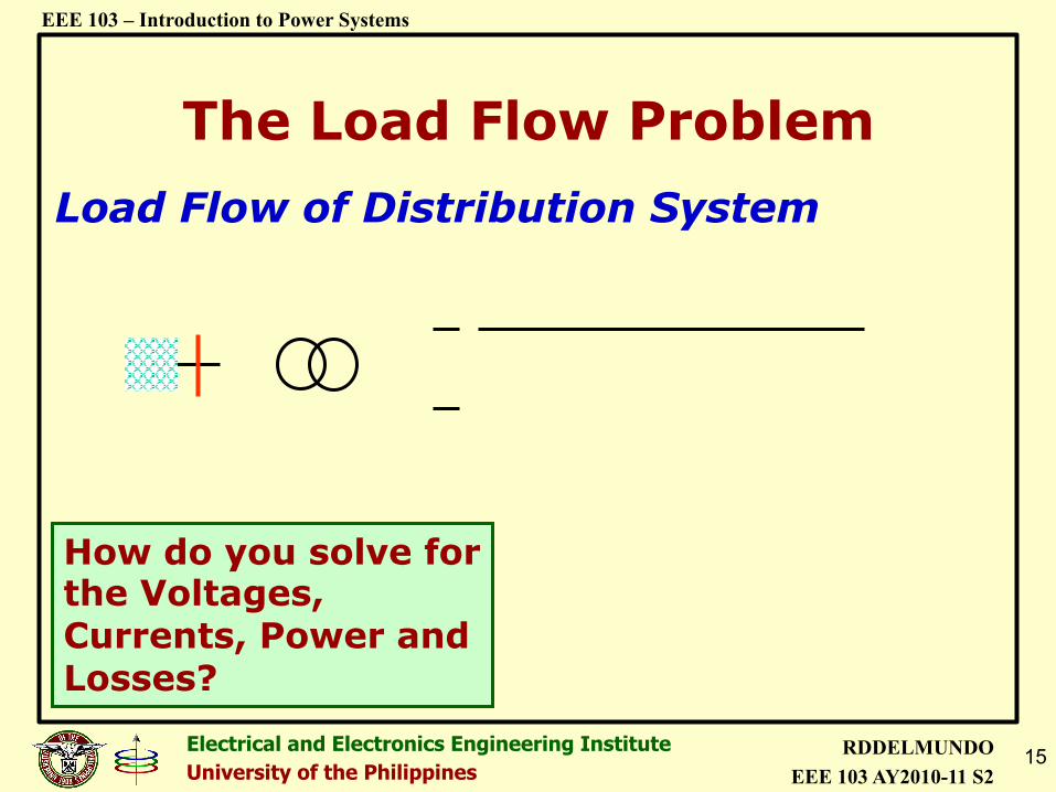
The Load Flow Problem Load Flow of Distribution System
How do you solve for the Voltages, Currents, Power and Losses?
Bus1
Utility Grid
Bus2 Bus3
Bus4 V1 = 67 kV
Lumped Load A 2 MVA 85%PF
Lumped Load B 1 MVA 85%PF
V2 = ?
V4 = ?
V3 = ? I23 , Loss23 = ?
I24 , Loss24 = ?
I12 , Loss12 = ?
P1 , Q1 = ? P2 , Q2 = ?
P3 , Q3 = ?
P4 , Q4 = ?
16 Electrical and Electronics Engineering Institute University of the Philippines
RDDELMUNDO EEE 103 AY2010-11 S2
EEE 103 – Introduction to Power Systems
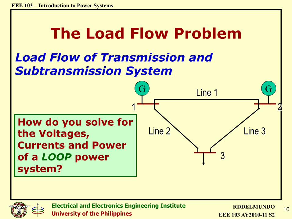
The Load Flow Problem
Line 1
Line 3 Line 2
1 2
3
G G
How do you solve for the Voltages, Currents and Power of a LOOP power system?
Load Flow of Transmission and Subtransmission System
17 Electrical and Electronics Engineering Institute University of the Philippines
RDDELMUNDO EEE 103 AY2010-11 S2
EEE 103 – Introduction to Power Systems
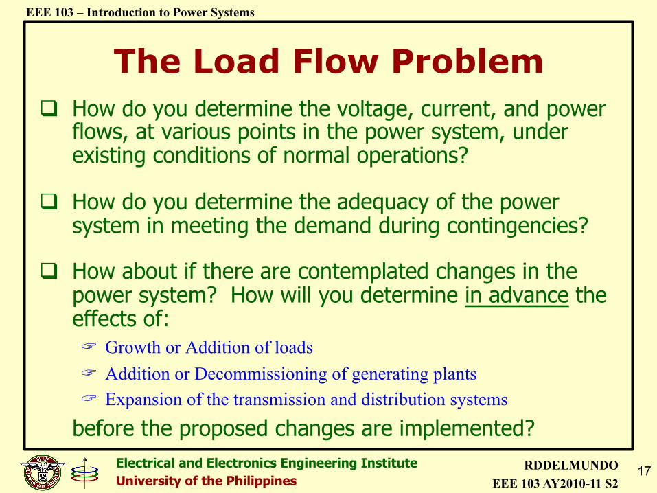
The Load Flow Problem ! How do you determine the voltage, current, and power
flows, at various points in the power system, under existing conditions of normal operations?
! How do you determine the adequacy of the power system in meeting the demand during contingencies?
! How about if there are contemplated changes in the power system? How will you determine in advance the effects of: ! Growth or Addition of loads ! Addition or Decommissioning of generating plants ! Expansion of the transmission and distribution systems
before the proposed changes are implemented?
18 Electrical and Electronics Engineering Institute University of the Philippines
RDDELMUNDO EEE 103 AY2010-11 S2
EEE 103 – Introduction to Power Systems
The Load Flow Problem
Load Flow Analysis simulates (i.e., mathematically
determines) the performance of an electric power system under a given set of conditions.
Load Flow (also called Power Flow) takes a snapshot of the electric power system at a given point in time.
ANSWER: THE LOAD FLOW STUDY!
19 Electrical and Electronics Engineering Institute University of the Philippines
RDDELMUNDO EEE 103 AY2010-11 S2
EEE 103 – Introduction to Power Systems
POWER SYSTEM MODELS FOR LOAD FLOW ANALYSIS
20 Electrical and Electronics Engineering Institute University of the Philippines
RDDELMUNDO EEE 103 AY2010-11 S2
EEE 103 – Introduction to Power Systems
Network Models
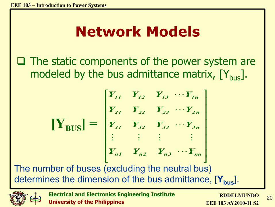
! The static components of the power system are modeled by the bus admittance matrix, [Ybus].
!!!!!!!!
"
#
$$$$$$$$
%
&
nn3n2n1n
n3333231
n2232221
n1131211
YYYY
YYYY
YYYY
YYYY
[YBUS] =
The number of buses (excluding the neutral bus) determines the dimension of the bus admittance, [Ybus].
21 Electrical and Electronics Engineering Institute University of the Philippines
RDDELMUNDO EEE 103 AY2010-11 S2
EEE 103 – Introduction to Power Systems
Generator Models
1. Voltage-controlled generating units to supply a scheduled active power P at a specified voltage magnitude V. The generators are equipped with voltage regulators to adjust the field excitation so that the units will supply or absorb a particular reactive power Q in order to maintain the voltage.
2. Swing generating units to maintain the frequency at 60Hz in addition to the specified voltage. The generating unit is equipped with frequency following controller (quick-responding speed governor) and is assigned as the Swing Generator.
22 Electrical and Electronics Engineering Institute University of the Philippines
RDDELMUNDO EEE 103 AY2010-11 S2
EEE 103 – Introduction to Power Systems
Bus Types
! The power system is interconnected through the busses. The busses must therefore be identified in the load flow model. ! Generators, shunt admittances, and loads are
connected from their corresponding bus to the neutral bus.
! Transmission lines, transformers, and series impedances are connected from bus to bus.
23 Electrical and Electronics Engineering Institute University of the Philippines
RDDELMUNDO EEE 103 AY2010-11 S2
EEE 103 – Introduction to Power Systems
Bus Types
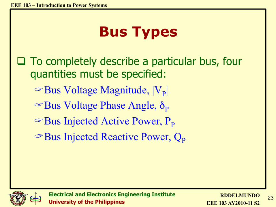
! To completely describe a particular bus, four quantities must be specified: ! Bus Voltage Magnitude, |VP| ! Bus Voltage Phase Angle, δP
! Bus Injected Active Power, PP
! Bus Injected Reactive Power, QP
24 Electrical and Electronics Engineering Institute University of the Philippines
RDDELMUNDO EEE 103 AY2010-11 S2
EEE 103 – Introduction to Power Systems
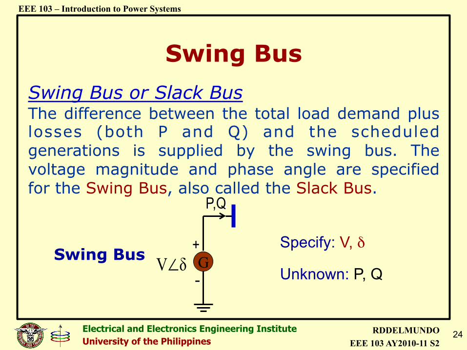
The difference between the total load demand plus losses (both P and Q) and the scheduled generations is supplied by the swing bus. The voltage magnitude and phase angle are specified for the Swing Bus, also called the Slack Bus.
Swing Bus Specify: V, δ
Unknown: P, Q G
P,Q
δV∠+
-
Swing Bus Swing Bus or Slack Bus
25 Electrical and Electronics Engineering Institute University of the Philippines
RDDELMUNDO EEE 103 AY2010-11 S2
EEE 103 – Introduction to Power Systems
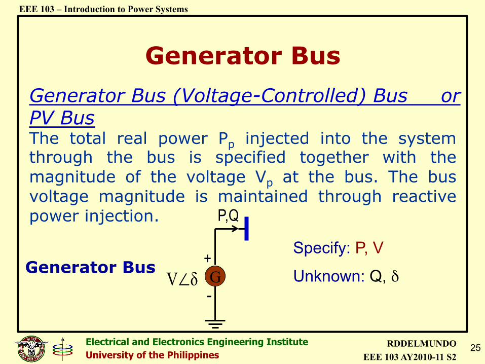
Generator Bus (Voltage-Controlled) Bus or PV Bus The total real power Pp injected into the system through the bus is specified together with the magnitude of the voltage Vp at the bus. The bus voltage magnitude is maintained through reactive power injection.
G
P,Q
δV∠+
- Generator Bus
Specify: P, V
Unknown: Q, δ
Generator Bus
26 Electrical and Electronics Engineering Institute University of the Philippines
RDDELMUNDO EEE 103 AY2010-11 S2
EEE 103 – Introduction to Power Systems
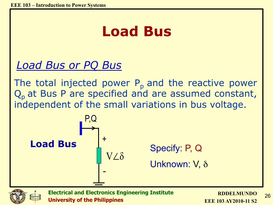
The total injected power Pp and the reactive power Qp at Bus P are specified and are assumed constant, independent of the small variations in bus voltage.
Load Bus or PQ Bus
P,Q
+
-
Load Bus Specify: P, Q
Unknown: V, δ δV∠
Load Bus
27 Electrical and Electronics Engineering Institute University of the Philippines
RDDELMUNDO EEE 103 AY2010-11 S2
EEE 103 – Introduction to Power Systems
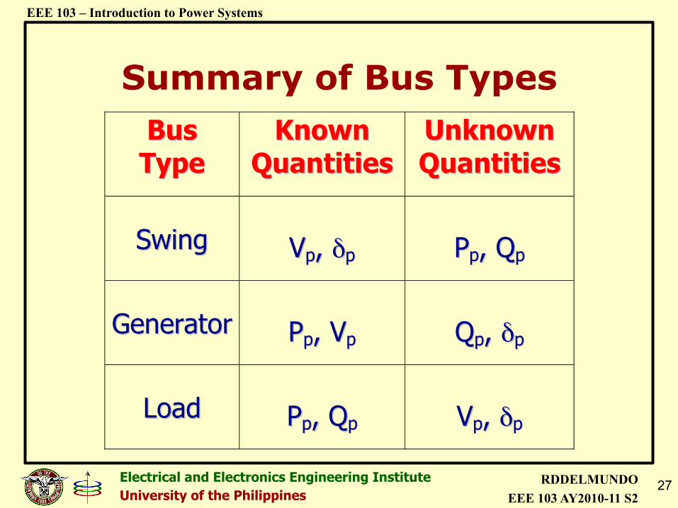
BBuuss TTyyppee
KKnnoowwnn QQuuaannttiittiieess
UUnnkknnoowwnn QQuuaannttiittiieess
SSwwiinngg
VVpp,, δδpp
PPpp,, QQpp
GGeenneerraattoorr
PPpp,, VVpp
QQpp,, δδpp
LLooaadd
PPpp,, QQpp
VVpp,, δδpp
Summary of Bus Types
28 Electrical and Electronics Engineering Institute University of the Philippines
RDDELMUNDO EEE 103 AY2010-11 S2
EEE 103 – Introduction to Power Systems
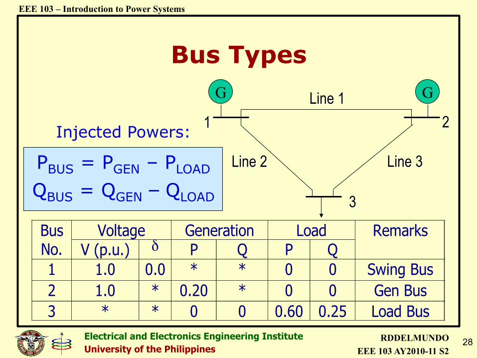
Line 1
Line 3 Line 2
1 2
3
G G
Voltage Generation Load Bus No. V (p.u.) δ P Q P Q
Remarks
1 1.0 0.0 * * 0 0 Swing Bus 2 1.0 * 0.20 * 0 0 Gen Bus 3 * * 0 0 0.60 0.25 Load Bus
PBUS = PGEN – PLOAD
Bus Types
QBUS = QGEN – QLOAD
Injected Powers:
29 Electrical and Electronics Engineering Institute University of the Philippines
RDDELMUNDO EEE 103 AY2010-11 S2
EEE 103 – Introduction to Power Systems
SOLUTIONS TO SIMULTANEOUS ALGEBRAIC EQUATIONS
30 Electrical and Electronics Engineering Institute University of the Philippines
RDDELMUNDO EEE 103 AY2010-11 S2
EEE 103 – Introduction to Power Systems
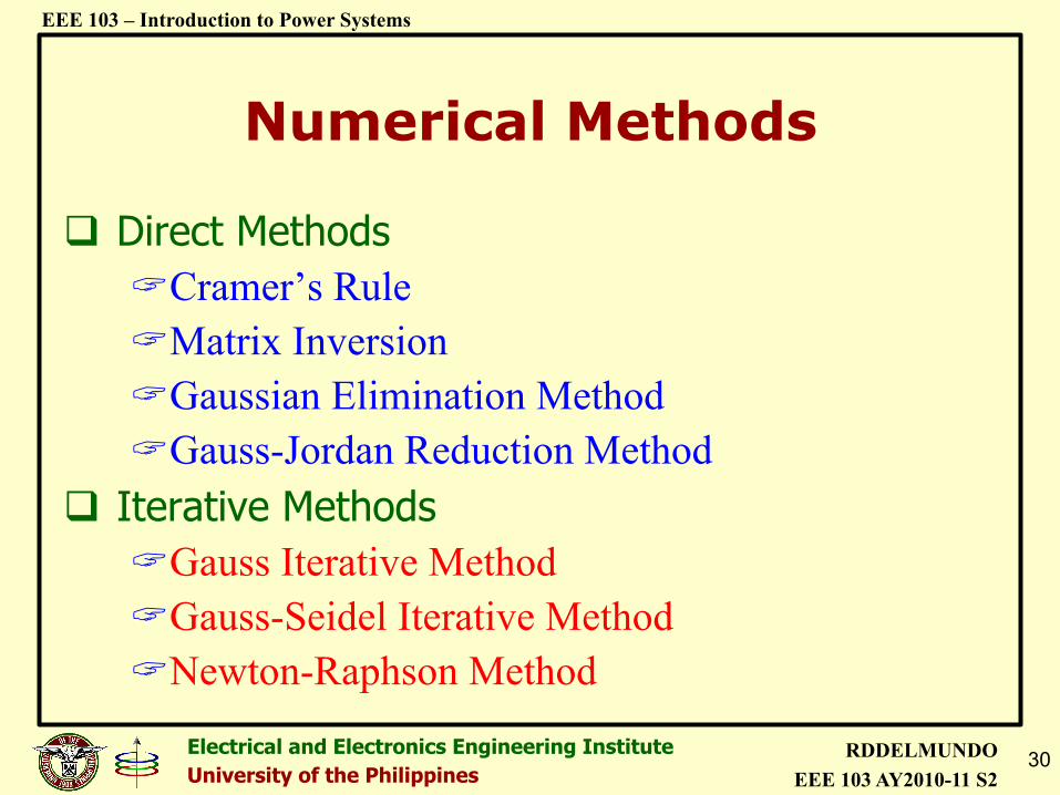
Numerical Methods
! Direct Methods ! Cramer’s Rule ! Matrix Inversion ! Gaussian Elimination Method ! Gauss-Jordan Reduction Method
! Iterative Methods ! Gauss Iterative Method ! Gauss-Seidel Iterative Method ! Newton-Raphson Method
31 Electrical and Electronics Engineering Institute University of the Philippines
RDDELMUNDO EEE 103 AY2010-11 S2
EEE 103 – Introduction to Power Systems
Iterative Methods
An iterative method (root word: iterate) is a repetitive process for obtaining the solution of an equation or a system of equations.
The solutions start from arbitrarily chosen initial estimates of the unknown variables from which a new set of estimates is determined.
Convergence is achieved when the absolute mismatch between the current and previous estimates is less than some acceptable pre-specified precision index (the convergence index) for all variables.
33 Electrical and Electronics Engineering Institute University of the Philippines
RDDELMUNDO EEE 103 AY2010-11 S2
EEE 103 – Introduction to Power Systems
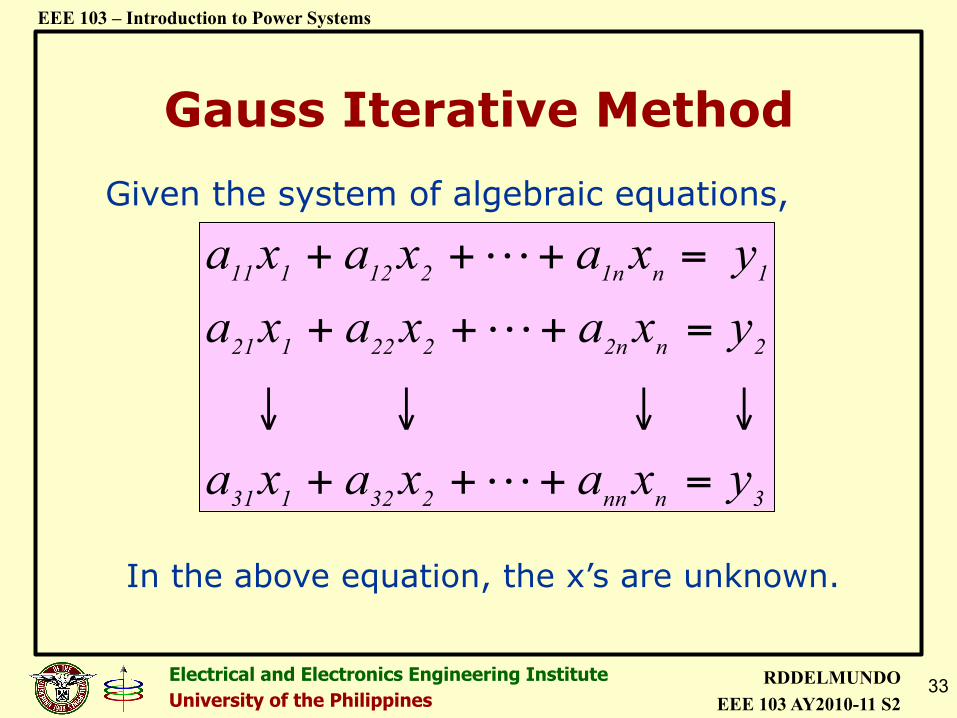
Given the system of algebraic equations,
In the above equation, the x’s are unknown.
3nnn232131
2n2n222121
1n1n212111
yxaxaxa
yxaxa xay xaxaxa
=+++
↓↓↓↓
=+++
=+++
Gauss Iterative Method
34 Electrical and Electronics Engineering Institute University of the Philippines
RDDELMUNDO EEE 103 AY2010-11 S2
EEE 103 – Introduction to Power Systems
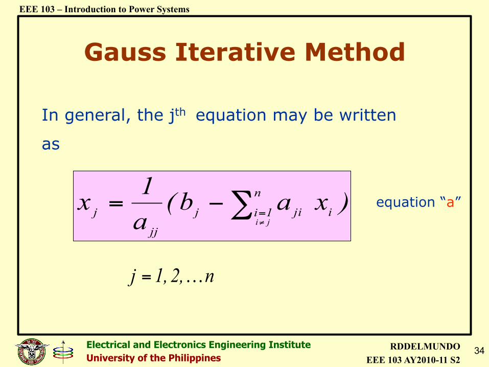
In general, the jth equation may be written
as
)xab(a1
x i
n
1i jij
jj
jji
∑≠=
−=
n 2, 1, j …=
equation “a”
Gauss Iterative Method
35 Electrical and Electronics Engineering Institute University of the Philippines
RDDELMUNDO EEE 103 AY2010-11 S2
EEE 103 – Introduction to Power Systems
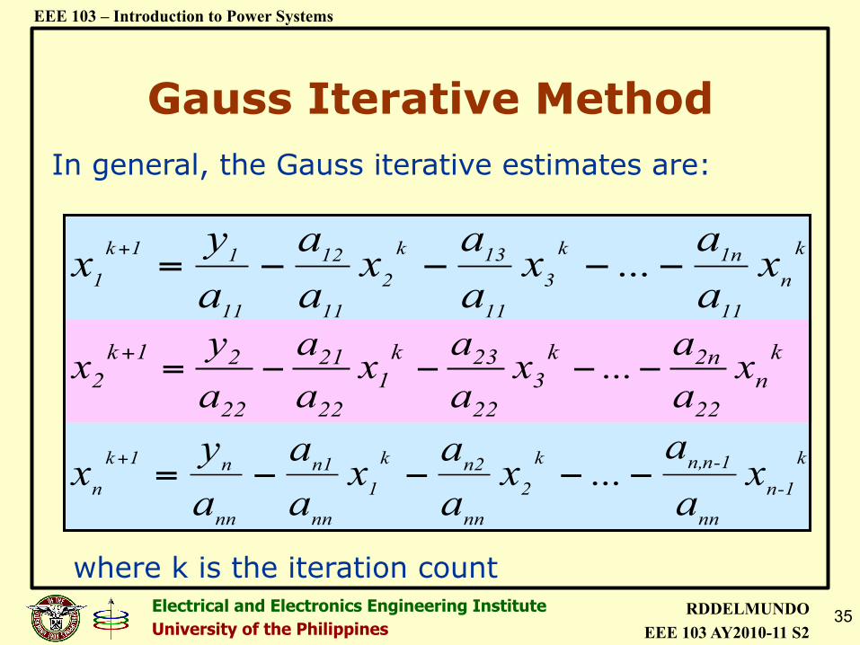
In general, the Gauss iterative estimates are:
where k is the iteration count
Gauss Iterative Method
k
n
11
1nk
3
11
13k
2
11
12
11
11k
1 xaa
...xaa
xaa
ayx −−−−=+
xaa
...xaa
xaa
ay
x kn
22
2nk3
22
23k1
22
21
22
21k2 −−−−=+
k
1-n
nn
1-nn,k
2
nn
n2k
1
nn
n1
nn
n1k
n xaa
...xaa
xaa
ay
x −−−−=+
36 Electrical and Electronics Engineering Institute University of the Philippines
RDDELMUNDO EEE 103 AY2010-11 S2
EEE 103 – Introduction to Power Systems
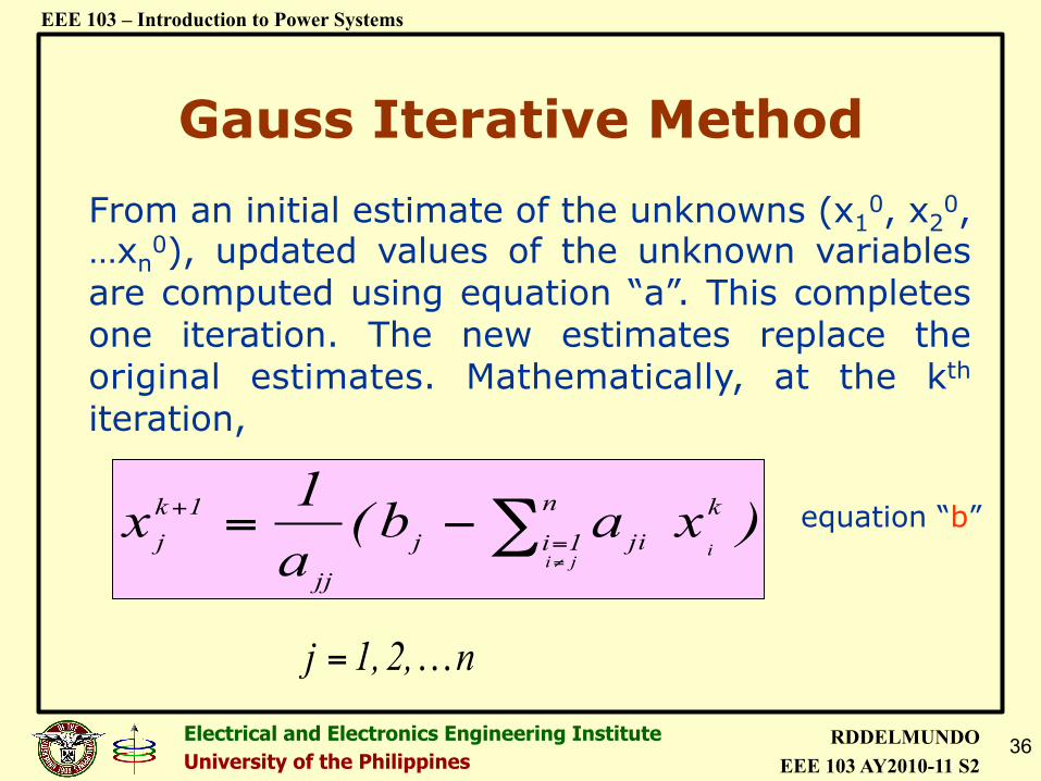
From an initial estimate of the unknowns (x10, x2
0,…xn
0), updated values of the unknown variables are computed using equation “a”. This completes one iteration. The new estimates replace the original estimates. Mathematically, at the kth iteration,
)xab(a1
x kn
1i jij
jj
1kj i
ji∑
≠=
+ −=
n 2, 1, j …=
equation “b”
Gauss Iterative Method
37 Electrical and Electronics Engineering Institute University of the Philippines
RDDELMUNDO EEE 103 AY2010-11 S2
EEE 103 – Introduction to Power Systems
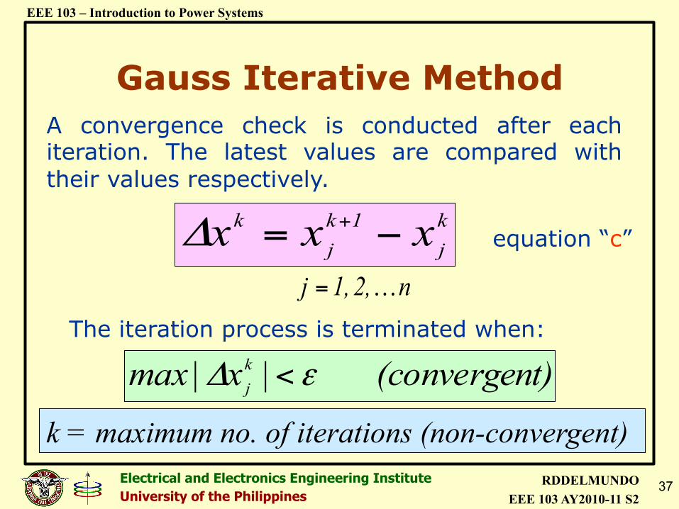
A convergence check is conducted after each iteration. The latest values are compared with their values respectively. k
j1k
jk xxx −= +Δ
n 2, 1, j …=
equation “c”
The iteration process is terminated when:
t)(convergen |x |max kj εΔ <
Gauss Iterative Method
k = maximum no. of iterations (non-convergent)
38 Electrical and Electronics Engineering Institute University of the Philippines
RDDELMUNDO EEE 103 AY2010-11 S2
EEE 103 – Introduction to Power Systems
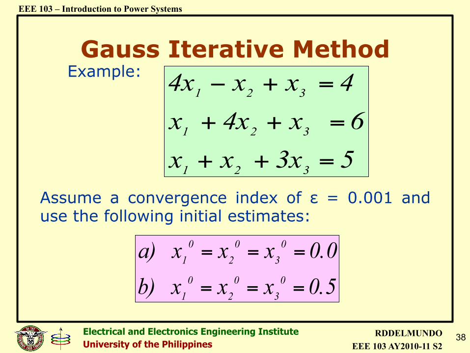
Example:
Assume a convergence index of ε = 0.001 and use the following initial estimates:
5 3x x x6 x 4x x
4 x x 4x
3 21
32 1
321
=++
=++
=+−
0.5 x x x b)
0.0 x x x a)0
30
20
1
0 3
0 2
0 1
===
===
Gauss Iterative Method
39 Electrical and Electronics Engineering Institute University of the Philippines
RDDELMUNDO EEE 103 AY2010-11 S2
EEE 103 – Introduction to Power Systems
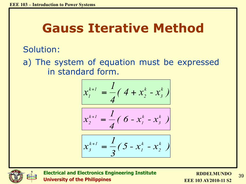
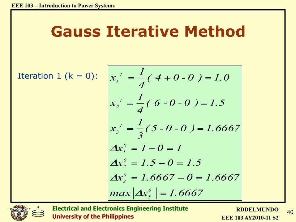
Solution: a) The system of equation must be expressed
in standard form.
)x- x 4 (41x k
3k2
1k1 +=+
Gauss Iterative Method
) x -x - 5(31x k
2k1
1k3 =+
) x - x - 6 ( 41x k
3k1
1k2 =+
40 Electrical and Electronics Engineering Institute University of the Philippines
RDDELMUNDO EEE 103 AY2010-11 S2
EEE 103 – Introduction to Power Systems
Iteration 1 (k = 0):
1.6667 x max
6667.106667.1x5.105.1x
101x
1.6667 ) 0 -0 - 5(31
x
1.5 ) 0 - 0 - 6 ( 41
x
1.0 ) 0 - 0 4 (41x
03
03
02
01
1 3
1 2
1 1
=
=−=
=−=
=−=
==
==
=+=
Δ
Δ
Δ
Δ
Gauss Iterative Method
41 Electrical and Electronics Engineering Institute University of the Philippines
RDDELMUNDO EEE 103 AY2010-11 S2
EEE 103 – Introduction to Power Systems
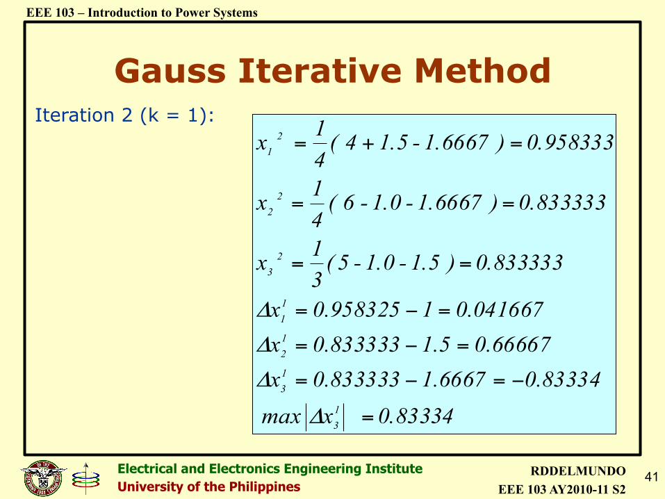
0.83334 x max
83334.06667.1833333.0x66667.05.1833333.0x
041667.01958325.0x
0.833333 ) 1.5 -1.0 - 5(31
x
0.833333 ) 1.6667 - 1.0 - 6 ( 41
x
0.958333 ) 1.6667 - 1.5 4 (41x
13
13
12
11
2 3
2 2
2 1
=
−=−=
=−=
=−=
==
==
=+=
Δ
Δ
Δ
Δ
Iteration 2 (k = 1):
Gauss Iterative Method
42 Electrical and Electronics Engineering Institute University of the Philippines
RDDELMUNDO EEE 103 AY2010-11 S2
EEE 103 – Introduction to Power Systems
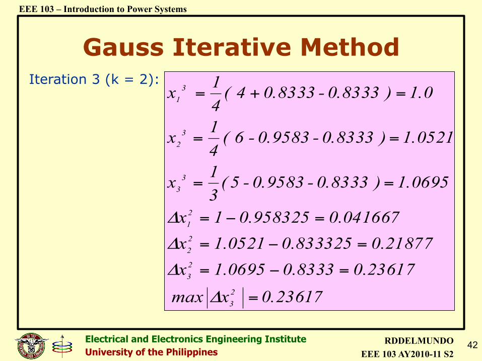
Iteration 3 (k = 2):
0.23617 x max
23617.08333.00695.1x21877.0833325.00521.1x
041667.0958325.01x
1.0695 ) 0.8333 -0.9583 - 5(31
x
1.0521 ) 0.8333 - 0.9583 - 6 ( 41
x
1.0 ) 0.8333 - 0.8333 4 (41x
23
23
22
21
3 3
3 2
3 1
=
=−=
=−=
=−=
==
==
=+=
Δ
Δ
Δ
Δ
Gauss Iterative Method
43 Electrical and Electronics Engineering Institute University of the Philippines
RDDELMUNDO EEE 103 AY2010-11 S2
EEE 103 – Introduction to Power Systems
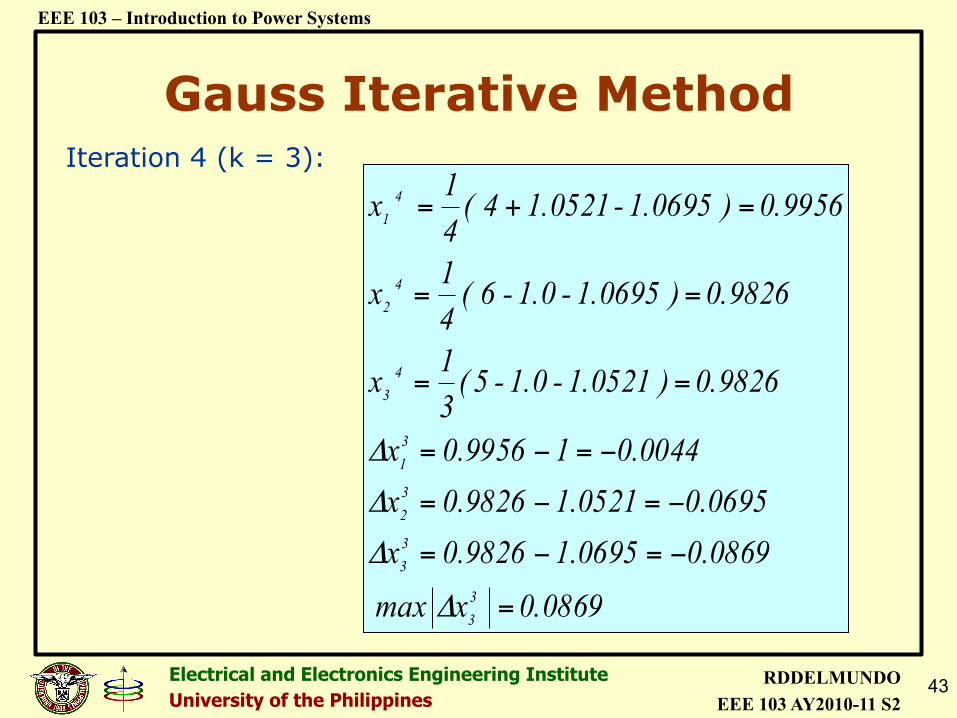
0.0869 x max
0869.00695.19826.0x0695.00521.19826.0x
0044.019956.0x
0.9826 ) 1.0521 -1.0 - 5(31
x
0.9826 ) 1.0695 - 1.0 - 6 ( 41
x
0.9956 ) 1.0695 - 1.0521 4 (41x
33
33
32
31
4 3
4 2
4 1
=
−=−=
−=−=
−=−=
==
==
=+=
Δ
Δ
Δ
Δ
Iteration 4 (k = 3):
Gauss Iterative Method
44 Electrical and Electronics Engineering Institute University of the Philippines
RDDELMUNDO EEE 103 AY2010-11 S2
EEE 103 – Introduction to Power Systems
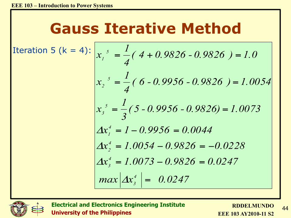
Iteration 5 (k = 4):
0.0247 x max
0247.09826.00073.1x0228.09826.00054.1x
0044.09956.01x
1.0073 0.9826) -0.9956 - 5(31
x
1.0054 ) 0.9826 - 0.9956 - 6 ( 41x
1.0 ) 0.9826 - 0.9826 4 (41
x
43
43
42
41
5 3
5 2
5 1
=
=−=
−=−=
=−=
==
==
=+=
Δ
Δ
Δ
Δ
Gauss Iterative Method
45 Electrical and Electronics Engineering Institute University of the Philippines
RDDELMUNDO EEE 103 AY2010-11 S2
EEE 103 – Introduction to Power Systems
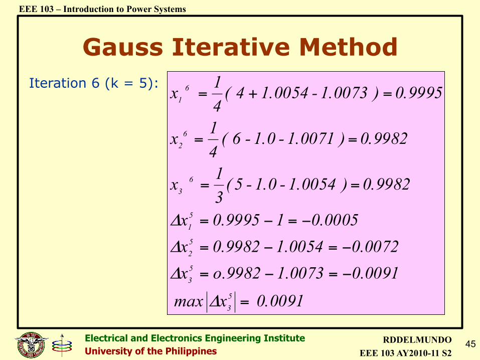
0.0091 x max
0091.00073.19982.ox0072.00054.19982.0x
0005.019995.0x
0.9982 ) 1.0054 -1.0 - 5(31
x
0.9982 ) 1.0071 - 1.0 - 6 ( 41
x
0.9995 ) 1.0073 - 1.0054 4 (41x
53
53
52
51
6 3
6 2
6 1
=
−=−=
−=−=
−=−=
==
==
=+=
Δ
Δ
Δ
Δ
Iteration 6 (k = 5):
Gauss Iterative Method
46 Electrical and Electronics Engineering Institute University of the Philippines
RDDELMUNDO EEE 103 AY2010-11 S2
EEE 103 – Introduction to Power Systems
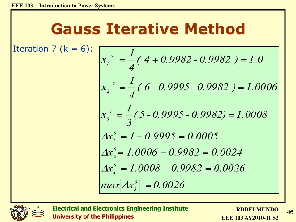
Iteration 7 (k = 6):
0.0026 xmax
0026.09982.00008.1x0024.09982.00006.1x
0005.09995.01x
1.0008 0.9982) -0.9995 - 5(31
x
1.0006 ) 0.9982 - 0.9995 - 6 ( 41
x
1.0 ) 0.9982 - 0.9982 4 (41x
63
63
62
61
7 3
7 2
7 1
=
=−=
=−=
=−=
==
==
=+=
Δ
Δ
Δ
Δ
Gauss Iterative Method
47 Electrical and Electronics Engineering Institute University of the Philippines
RDDELMUNDO EEE 103 AY2010-11 S2
EEE 103 – Introduction to Power Systems
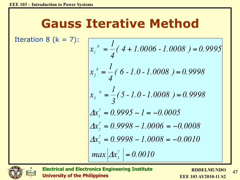
0.0010 x max
0010.00008.19998.0x0008.00006.19998.0x
0005.019995.0x
0.9998 ) 1.0008 -1.0 - 5(31
x
0.9998 ) 1.0008 - 1.0 - 6 ( 41x
0.9995 ) 1.0008 - 1.0006 4 (41
x
73
73
72
71
8 3
8 2
8 1
=
−=−=
−=−=
−=−=
==
==
=+=
Δ
Δ
Δ
Δ
Iteration 8 (k = 7):
Gauss Iterative Method
48 Electrical and Electronics Engineering Institute University of the Philippines
RDDELMUNDO EEE 103 AY2010-11 S2
EEE 103 – Introduction to Power Systems
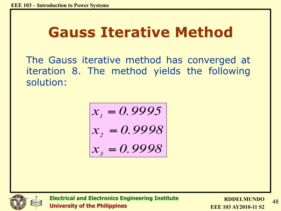
The Gauss iterative method has converged at iteration 8. The method yields the following solution:
0.9998 x0.9998 x
0.9995 x
3
2
1
=
=
=
Gauss Iterative Method
49 Electrical and Electronics Engineering Institute University of the Philippines
RDDELMUNDO EEE 103 AY2010-11 S2
EEE 103 – Introduction to Power Systems
GAUSS-SEIDEL ITERATIVE METHOD
FOR A SYSTEM OF EQUATIONS
50 Electrical and Electronics Engineering Institute University of the Philippines
RDDELMUNDO EEE 103 AY2010-11 S2
EEE 103 – Introduction to Power Systems
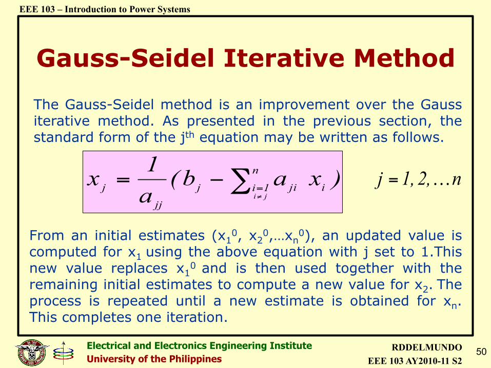
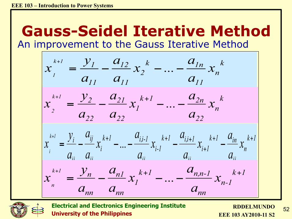
The Gauss-Seidel method is an improvement over the Gauss iterative method. As presented in the previous section, the standard form of the jth equation may be written as follows.
)xab(a1
x i
n
1i jij
jj
jji
∑≠=
−= n 2, 1, j …=
From an initial estimates (x10, x2
0,…xn0), an updated value is
computed for x1 using the above equation with j set to 1.This new value replaces x1
0 and is then used together with the remaining initial estimates to compute a new value for x2. The process is repeated until a new estimate is obtained for xn. This completes one iteration.
Gauss-Seidel Iterative Method
51 Electrical and Electronics Engineering Institute University of the Philippines
RDDELMUNDO EEE 103 AY2010-11 S2
EEE 103 – Introduction to Power Systems
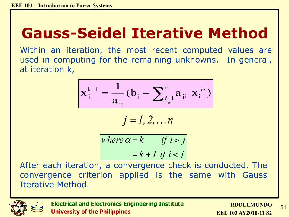
Within an iteration, the most recent computed values are used in computing for the remaining unknowns. In general, at iteration k,
i j
nk+1j j ji i1
jj
1x (b a x )
a iα
≠=
= −∑
n 2, 1, j …=
j i if 1k j i if k where
<+=
>=α
After each iteration, a convergence check is conducted. The convergence criterion applied is the same with Gauss Iterative Method.
Gauss-Seidel Iterative Method
52 Electrical and Electronics Engineering Institute University of the Philippines
RDDELMUNDO EEE 103 AY2010-11 S2
EEE 103 – Introduction to Power Systems
An improvement to the Gauss Iterative Method Gauss-Seidel Iterative Method
xaa
...xaa
ay
x kn
11
1nk2
11
12
11
11k
1−−−=
+
xaa
...xaa
ay
x kn
22
2n1k1
22
21
22
21k
2−−−= ++
1kn
ii
in1k1i
ii
1ii,1k1-i
ii
1-ii,1ki
ii
ij
ii
i xaa
xaa
xaa
...xaa
ay
x1k
i
+++
+++ −−−−−=+
xa
a...x
aa
ay
x 1k1-n
nn
1-nn,1k1
nn
n1
nn
n1k
n
++ −−−=+
53 Electrical and Electronics Engineering Institute University of the Philippines
RDDELMUNDO EEE 103 AY2010-11 S2
EEE 103 – Introduction to Power Systems
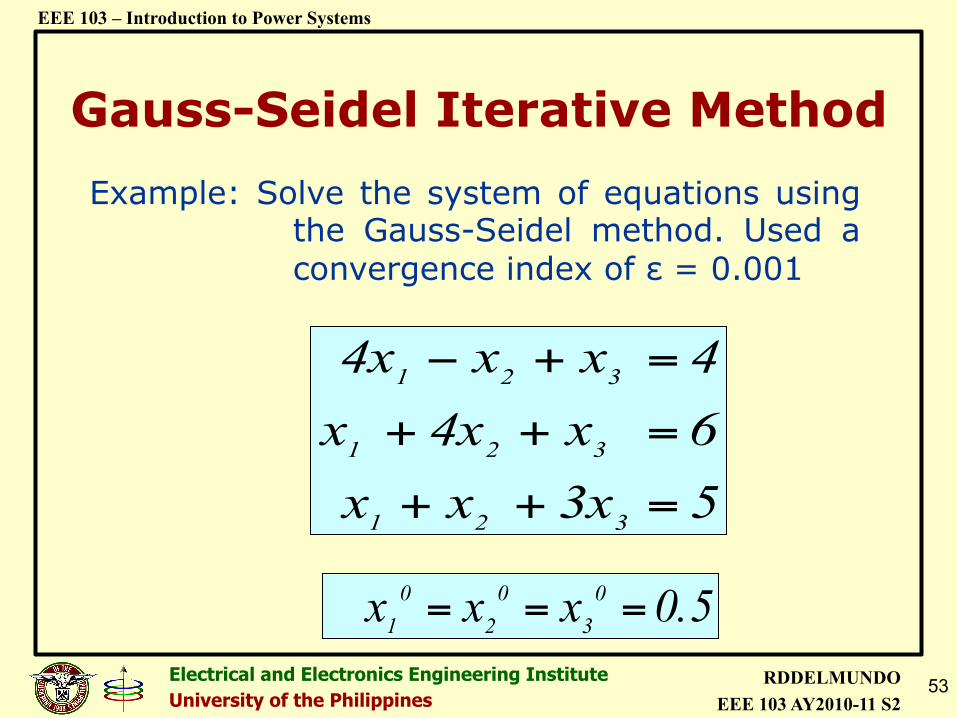
Example: Solve the system of equations using the Gauss-Seidel method. Used a convergence index of ε = 0.001
5 3x x x6 x 4x x4 x x 4x
3 21
32 1
321
=++
=++
=+−
0.5 x x x 0 3
0 2
0 1 ===
Gauss-Seidel Iterative Method
54 Electrical and Electronics Engineering Institute University of the Philippines
RDDELMUNDO EEE 103 AY2010-11 S2
EEE 103 – Introduction to Power Systems
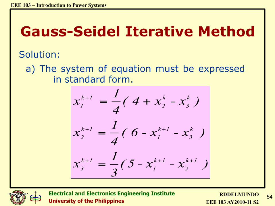
Solution: a) The system of equation must be expressed
in standard form.
) x -x - 5(31x
) x - x - 6 ( 41x
)x- x 4 (41x
1k2
1k1
1k3
k3
1k1
1k2
k3
k2
1k1
+++
++
+
=
=
+=
Gauss-Seidel Iterative Method
55 Electrical and Electronics Engineering Institute University of the Philippines
RDDELMUNDO EEE 103 AY2010-11 S2
EEE 103 – Introduction to Power Systems
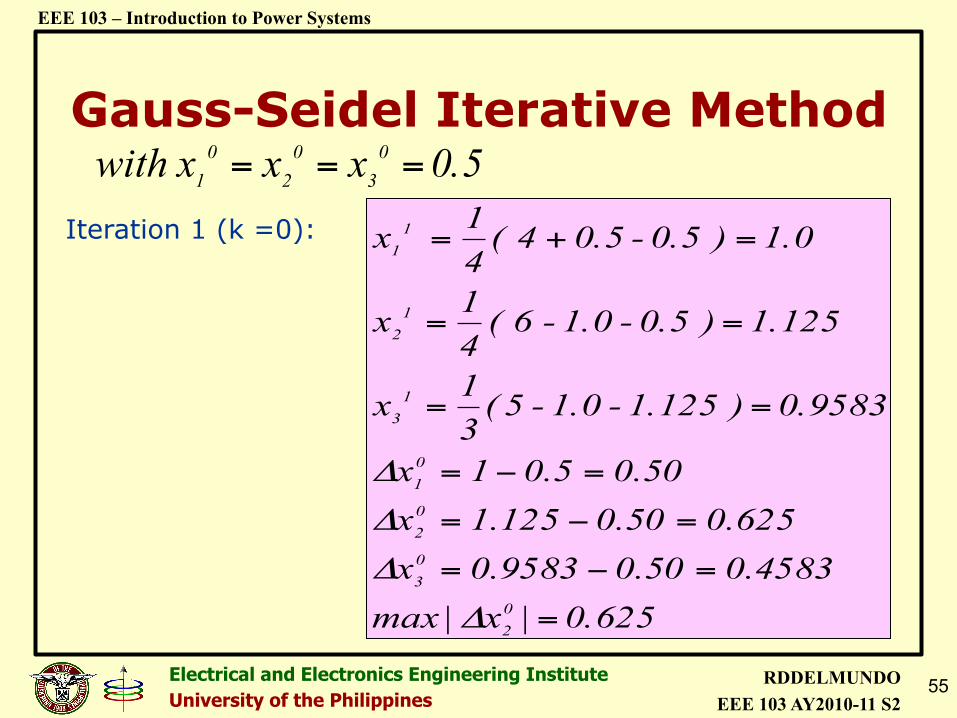
Iteration 1 (k =0):
0.625 | x |max
4583.050.09583.0x625.050.0125.1x
50.05.01x
0.9583 ) 1.125 -1.0 - 5(31x
1.125 ) 0.5 - 1.0 - 6 ( 41
x
1.0 ) 0.5 - 0.5 4 (41
x
02
03
02
01
1 3
1 2
1 1
=
=−=
=−=
=−=
==
==
=+=
Δ
Δ
Δ
Δ
0.5 x x x with 0 3
0 2
0 1 ===
Gauss-Seidel Iterative Method
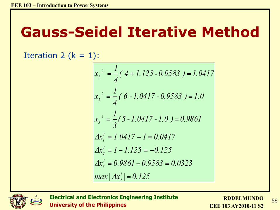
56 Electrical and Electronics Engineering Institute University of the Philippines
RDDELMUNDO EEE 103 AY2010-11 S2
EEE 103 – Introduction to Power Systems
0.125 | x |max
0323.09583.09861.0x125.0125.11x0417.010417.1x
0.9861 ) 1.0 -1.0417 - 5(31x
1.0 ) 0.9583 - 1.0417 - 6 ( 41
x
1.0417 ) 0.9583 - 1.125 4 (41
x
12
13
12
11
2 3
2 2
2 1
=
=−=
−=−=
=−=
==
==
=+=
Δ
Δ
Δ
Δ
Iteration 2 (k = 1):
Gauss-Seidel Iterative Method
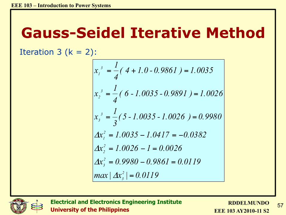
57 Electrical and Electronics Engineering Institute University of the Philippines
RDDELMUNDO EEE 103 AY2010-11 S2
EEE 103 – Introduction to Power Systems
Iteration 3 (k = 2):
0.0119 | x |max
0119.09861.09980.0x0026.010026.1x
0382.00417.10035.1x
0.9980 ) 1.0026 -1.0035 - 5(31x
1.0026 ) 0.9891 - 1.0035 - 6 ( 41
x
1.0035 ) 0.9861 - 1.0 4 (41x
23
23
22
21
3 3
3 2
3 1
=
=−=
=−=
−=−=
==
==
=+=
Δ
Δ
Δ
Δ
Gauss-Seidel Iterative Method
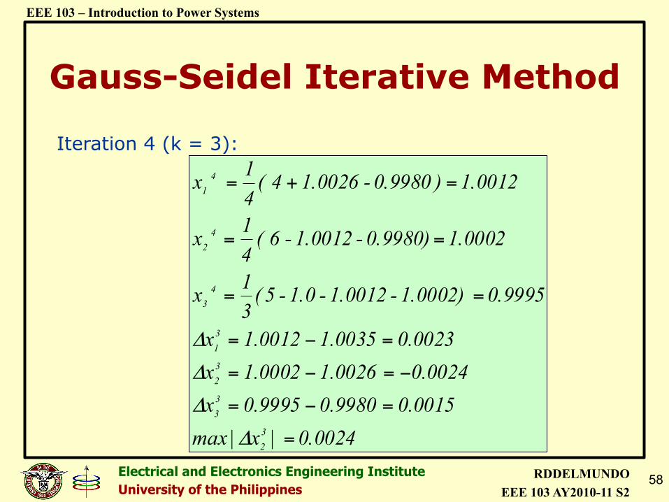
58 Electrical and Electronics Engineering Institute University of the Philippines
RDDELMUNDO EEE 103 AY2010-11 S2
EEE 103 – Introduction to Power Systems
0.0024 | x |max
0015.09980.09995.0x0024.00026.10002.1x
0023.00035.10012.1x
0.9995 1.0002) -1.0012 -1.0 - 5(31x
1.0002 0.9980) - 1.0012 - 6 ( 41
x
1.0012 )0.9980 -1.0026 4 (41
x
32
33
32
31
4 3
4 2
4 1
=
=−=
−=−=
=−=
==
==
=+=
Δ
Δ
Δ
Δ
Iteration 4 (k = 3):
Gauss-Seidel Iterative Method
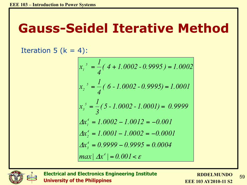
59 Electrical and Electronics Engineering Institute University of the Philippines
RDDELMUNDO EEE 103 AY2010-11 S2
EEE 103 – Introduction to Power Systems
Iteration 5 (k = 4):
εΔ
Δ
Δ
Δ
0.001 | x|max
0004.09995.09999.0x0001.00002.10001.1x001.00012.10002.1x
0.9999 1.0001) -1.0002 - 5(31x
1.0001 0.9995) - 1.0002 - 6 ( 41
x
1.0002 )0.9995 - 1.0002 4 (41
x
4
43
42
41
5 3
5 2
5 1
<=
=−=
−=−=
−=−=
==
==
=+=
Gauss-Seidel Iterative Method
60 Electrical and Electronics Engineering Institute University of the Philippines
RDDELMUNDO EEE 103 AY2010-11 S2
EEE 103 – Introduction to Power Systems
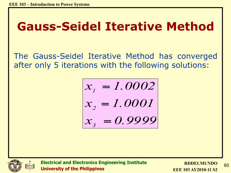
The Gauss-Seidel Iterative Method has converged after only 5 iterations with the following solutions:
0.9999 x1.0001 x1.0002 x
3
2
1
=
=
=
Gauss-Seidel Iterative Method
62 Electrical and Electronics Engineering Institute University of the Philippines
RDDELMUNDO EEE 103 AY2010-11 S2
EEE 103 – Introduction to Power Systems
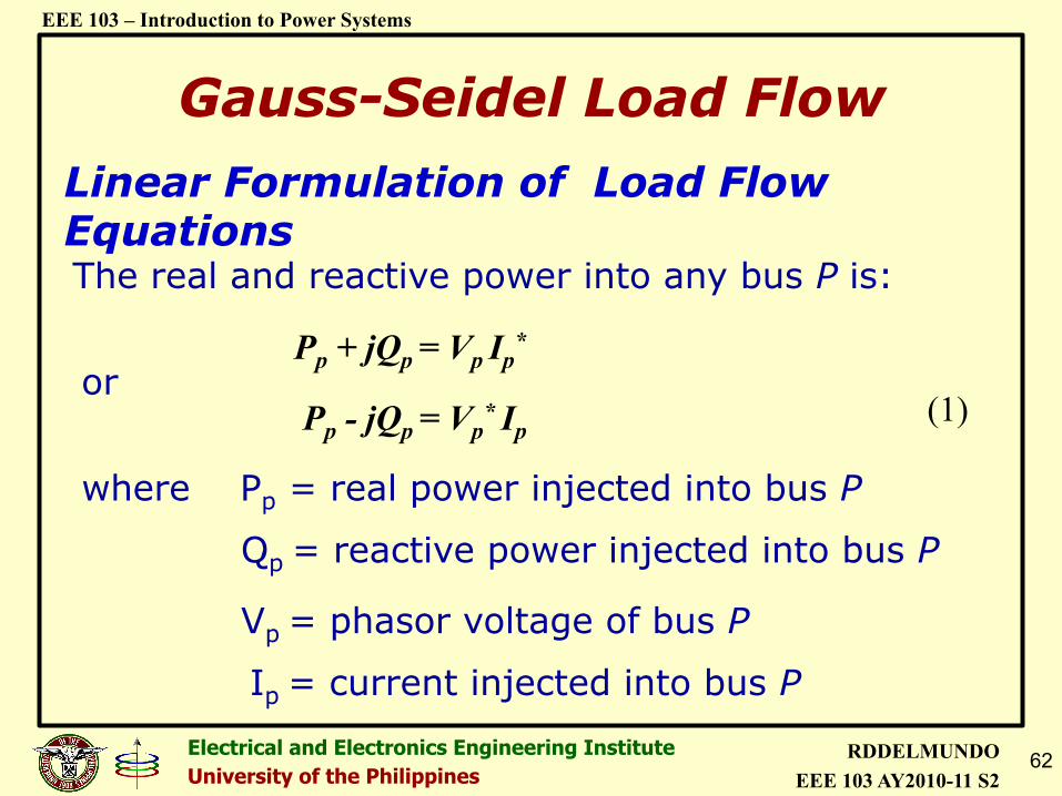
The real and reactive power into any bus P is:
Pp + jQp = Vp Ip*
where Pp = real power injected into bus P
Qp = reactive power injected into bus P
Vp = phasor voltage of bus P
Ip = current injected into bus P
Pp - jQp = Vp* Ip
or
Gauss-Seidel Load Flow
(1)
Linear Formulation of Load Flow Equations
63 Electrical and Electronics Engineering Institute University of the Philippines
RDDELMUNDO EEE 103 AY2010-11 S2
EEE 103 – Introduction to Power Systems
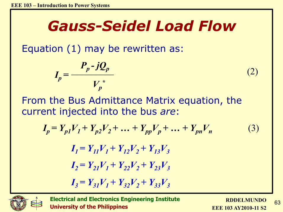
Equation (1) may be rewritten as:
Ip = Pp - jQp _________
Vp*
From the Bus Admittance Matrix equation, the current injected into the bus are:
I1 = Y11V1 + Y12V2 + Y13V3
I2 = Y21V1 + Y22V2 + Y23V3
I3 = Y31V1 + Y32V2 + Y33V3
Gauss-Seidel Load Flow
(2)
(3) Ip = Yp1V1 + Yp2V2 + … + YppVp + … + YpnVn
64 Electrical and Electronics Engineering Institute University of the Philippines
RDDELMUNDO EEE 103 AY2010-11 S2
EEE 103 – Introduction to Power Systems
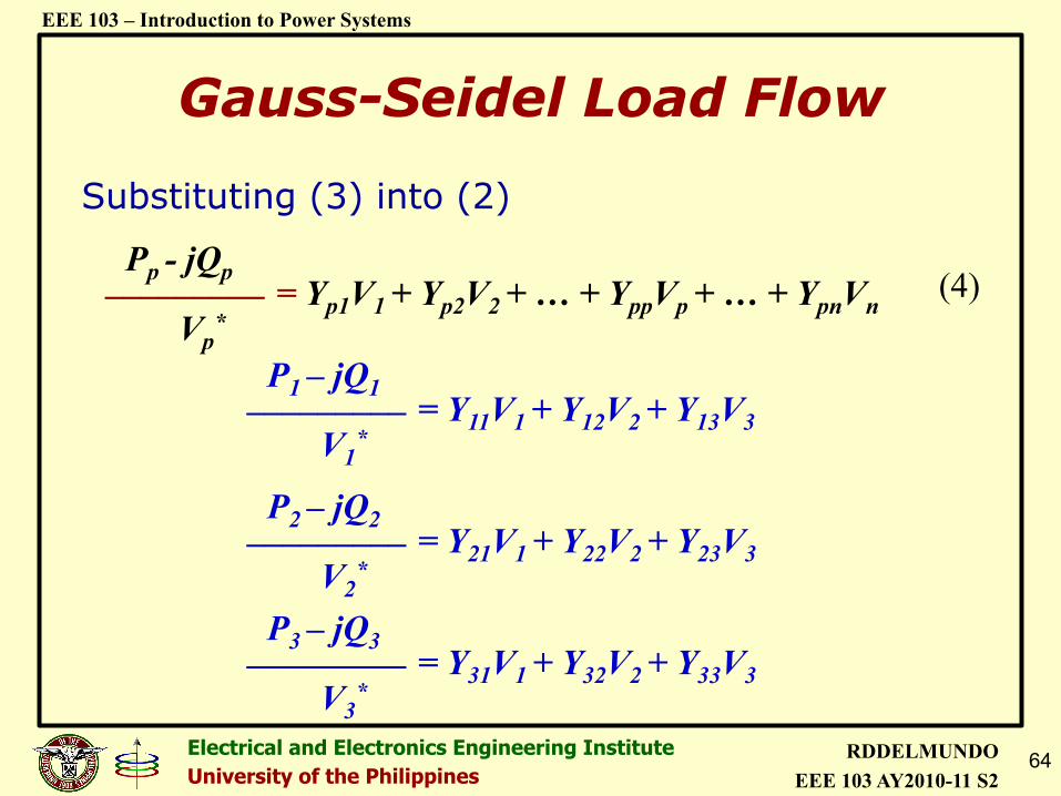
Substituting (3) into (2)
_________ Vp
*
Pp - jQp = Yp1V1 + Yp2V2 + … + YppVp + … + YpnVn
Gauss-Seidel Load Flow
_________ V1
*
P1 – jQ1 = Y11V1 + Y12V2 + Y13V3
_________ V2
*
P2 – jQ2 = Y21V1 + Y22V2 + Y23V3
_________ V3
*
P3 – jQ3 = Y31V1 + Y32V2 + Y33V3
(4)
65 Electrical and Electronics Engineering Institute University of the Philippines
RDDELMUNDO EEE 103 AY2010-11 S2
EEE 103 – Introduction to Power Systems
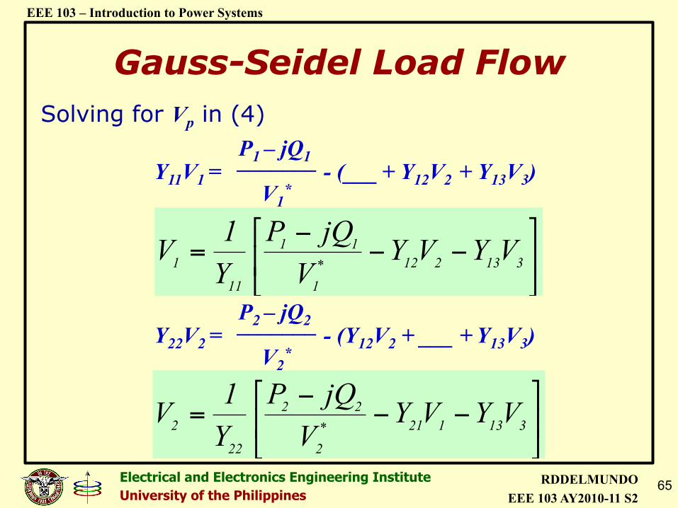
Solving for Vp in (4)
_______ Y11V1 = P1 – jQ1
V1*
- (___ + Y12V2 + Y13V3)
Gauss-Seidel Load Flow
!"
#$%
&−−
−= 313212*
1
11
11
1 VYVYVjQP
Y1V
_______ Y22V2 = P2 – jQ2
V2*
- (Y12V2 + ___ + Y13V3)
!"
#$%
&−−
−= 313121*
2
22
22
2 VYVYVjQP
Y1V
66 Electrical and Electronics Engineering Institute University of the Philippines
RDDELMUNDO EEE 103 AY2010-11 S2
EEE 103 – Introduction to Power Systems
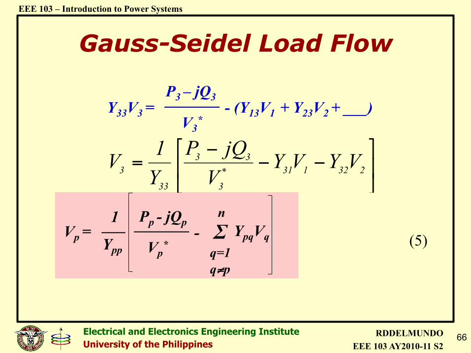
Gauss-Seidel Load Flow
!"
#$%
&−−
−= 232131*
3
33
33
3 VYVYVjQP
Y1V
_______ Y33V3 = P3 – jQ3
V3*
- (Y13V1 + Y23V2 + ___)
(5) Vp =
1 ___ Ypp
_______ Vp
*
Pp - jQp Σ - n
q=1 q≠p
YpqVq
67 Electrical and Electronics Engineering Institute University of the Philippines
RDDELMUNDO EEE 103 AY2010-11 S2
EEE 103 – Introduction to Power Systems
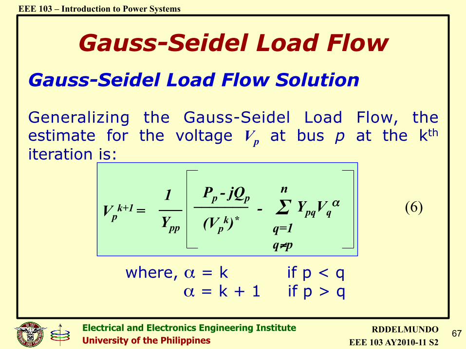
Generalizing the Gauss-Seidel Load Flow, the estimate for the voltage Vp at bus p at the kth iteration is:
Vpk+1
=
1 ___ Ypp
_______ (Vp
k)*
Pp - jQp Σ - n
q=1 q≠p
YpqVqα
where, α = k if p < q α = k + 1 if p > q
Gauss-Seidel Load Flow Gauss-Seidel Load Flow Solution
(6)
68 Electrical and Electronics Engineering Institute University of the Philippines
RDDELMUNDO EEE 103 AY2010-11 S2
EEE 103 – Introduction to Power Systems
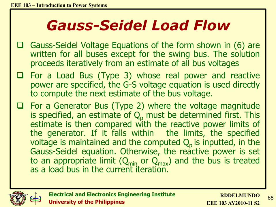
! Gauss-Seidel Voltage Equations of the form shown in (6) are written for all buses except for the swing bus. The solution proceeds iteratively from an estimate of all bus voltages
! For a Load Bus (Type 3) whose real power and reactive power are specified, the G-S voltage equation is used directly to compute the next estimate of the bus voltage.
! For a Generator Bus (Type 2) where the voltage magnitude is specified, an estimate of Qp must be determined first. This estimate is then compared with the reactive power limits of the generator. If it falls within the limits, the specified voltage is maintained and the computed Qp is inputted, in the Gauss-Seidel equation. Otherwise, the reactive power is set to an appropriate limit (Qmin or Qmax) and the bus is treated as a load bus in the current iteration.
Gauss-Seidel Load Flow
69 Electrical and Electronics Engineering Institute University of the Philippines
RDDELMUNDO EEE 103 AY2010-11 S2
EEE 103 – Introduction to Power Systems
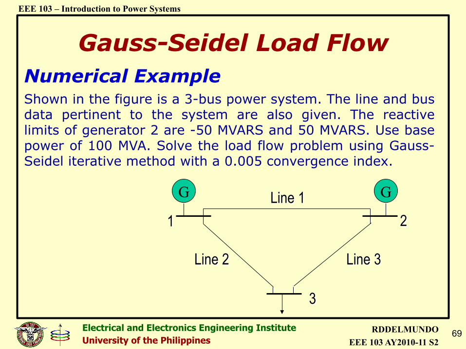
Numerical Example Shown in the figure is a 3-bus power system. The line and bus data pertinent to the system are also given. The reactive limits of generator 2 are -50 MVARS and 50 MVARS. Use base power of 100 MVA. Solve the load flow problem using Gauss-Seidel iterative method with a 0.005 convergence index.
Line 1
Line 3 Line 2
1 2
3
G G
Gauss-Seidel Load Flow
70 Electrical and Electronics Engineering Institute University of the Philippines
RDDELMUNDO EEE 103 AY2010-11 S2
EEE 103 – Introduction to Power Systems
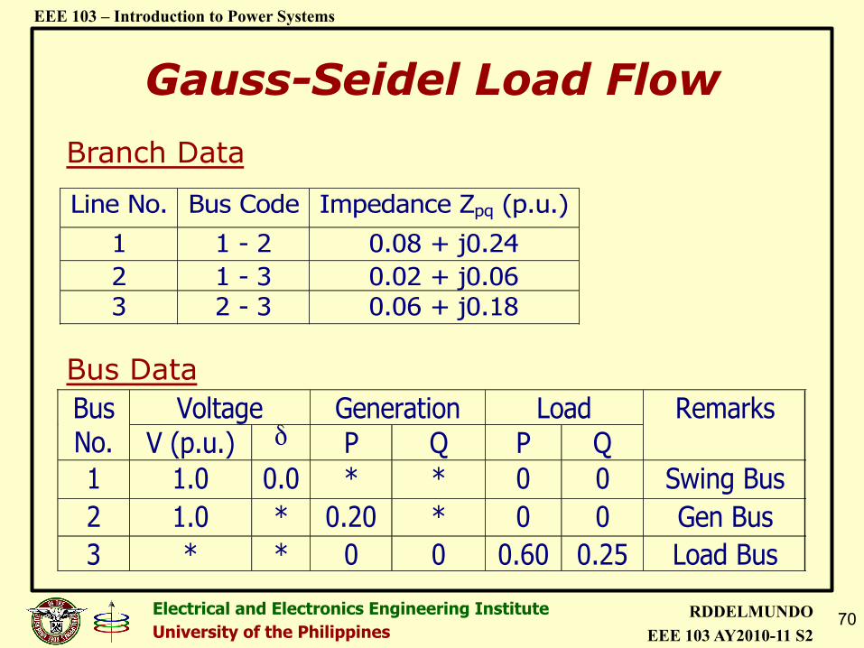
Branch Data
Line No. Bus Code Impedance Zpq (p.u.)
1 1 - 2 0.08 + j0.24 2 1 - 3 0.02 + j0.06 3 2 - 3 0.06 + j0.18
Bus Data Voltage Generation Load Bus
No. V (p.u.) δ P Q P Q Remarks
1 1.0 0.0 * * 0 0 Swing Bus 2 1.0 * 0.20 * 0 0 Gen Bus 3 * * 0 0 0.60 0.25 Load Bus
Gauss-Seidel Load Flow
71 Electrical and Electronics Engineering Institute University of the Philippines
RDDELMUNDO EEE 103 AY2010-11 S2
EEE 103 – Introduction to Power Systems
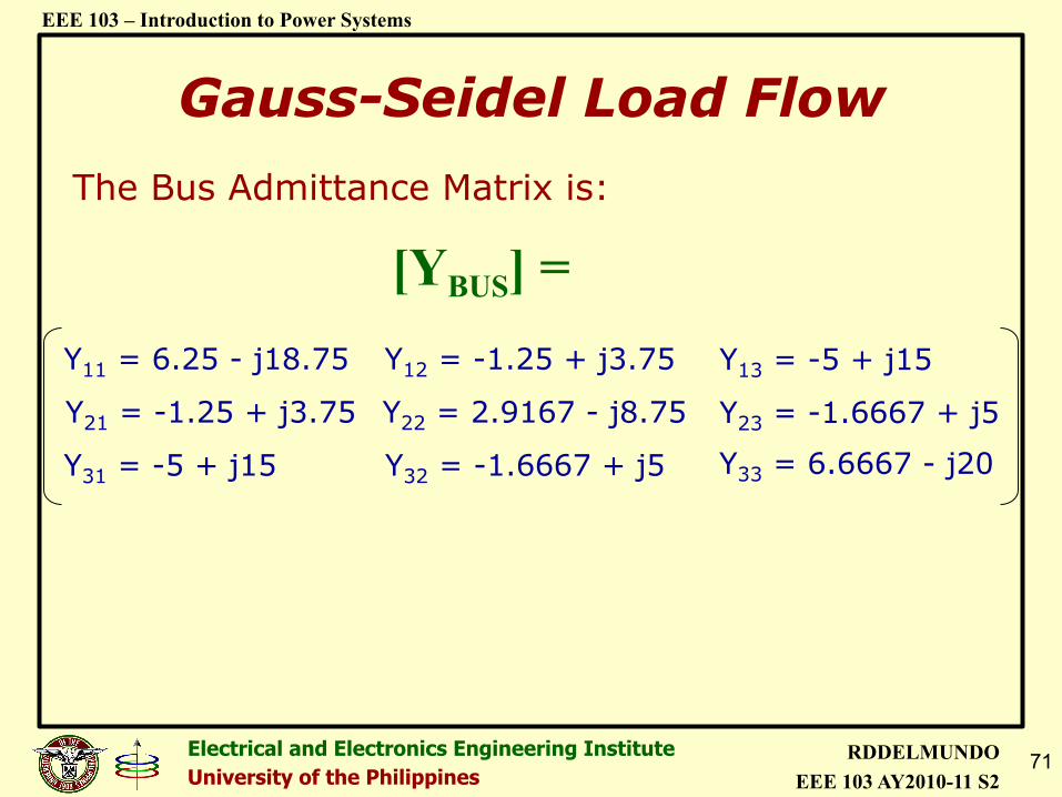
The Bus Admittance Matrix is:
Gauss-Seidel Load Flow
Y11 = 6.25 - j18.75
Y21 = -1.25 + j3.75
Y31 = -5 + j15
Y12 = -1.25 + j3.75
Y22 = 2.9167 - j8.75
Y32 = -1.6667 + j5 Y33 = 6.6667 - j20
Y13 = -5 + j15
Y23 = -1.6667 + j5
[YBUS] =
72 Electrical and Electronics Engineering Institute University of the Philippines
RDDELMUNDO EEE 103 AY2010-11 S2
EEE 103 – Introduction to Power Systems
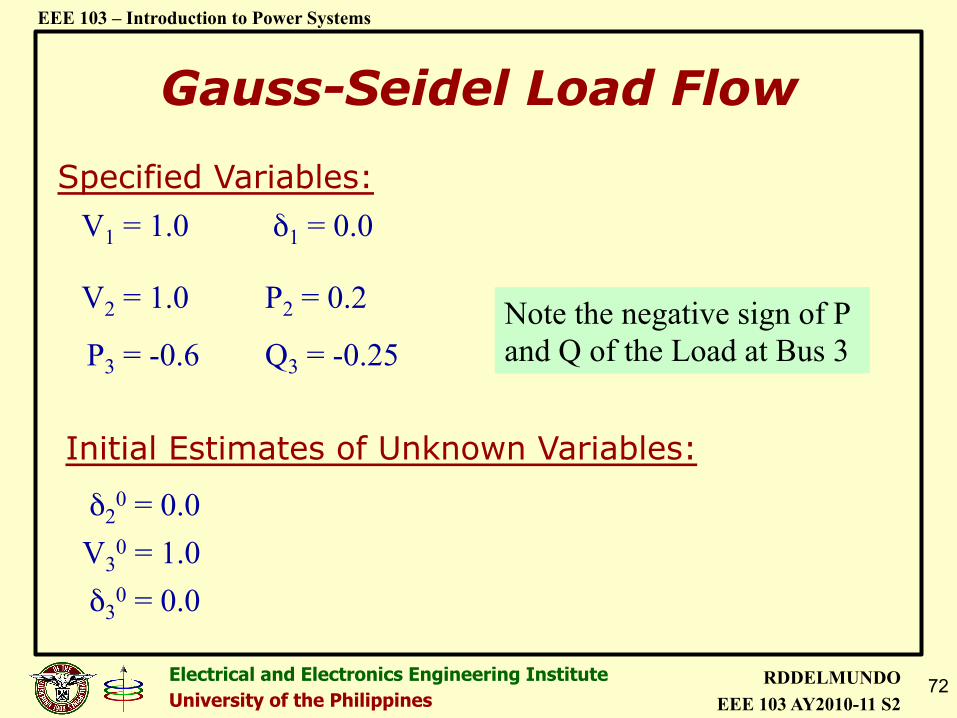
Specified Variables: V1 = 1.0 δ1 = 0.0
V2 = 1.0 P2 = 0.2
P3 = -0.6 Q3 = -0.25
Initial Estimates of Unknown Variables:
δ20 = 0.0
V30 = 1.0
δ30 = 0.0
Note the negative sign of P and Q of the Load at Bus 3
Gauss-Seidel Load Flow
73 Electrical and Electronics Engineering Institute University of the Philippines
RDDELMUNDO EEE 103 AY2010-11 S2
EEE 103 – Introduction to Power Systems
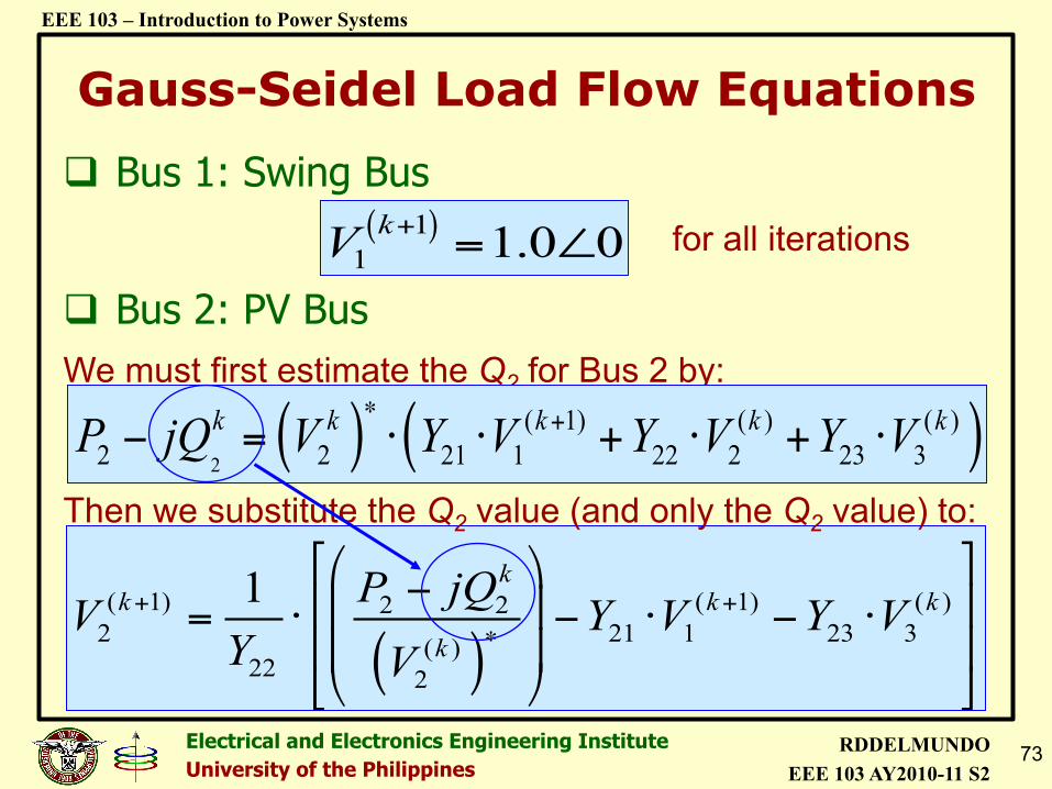
Gauss-Seidel Load Flow Equations
! Bus 1: Swing Bus
! Bus 2: PV Bus
for all iterations ( )11 1.0 0kV + = ∠
We must first estimate the Q2 for Bus 2 by:
( ) ( )2
( 1) ( ) ( )2 2 21 1 22 2 23 3
k k k k kP jQ V Y V Y V Y V∗ +− = ⋅ ⋅ + ⋅ + ⋅
( )( 1) ( 1) ( )2 22 21 1 23 3( )
22 2
1 kk k k
k
P jQV Y V Y VY V
+ +∗
" #$ %−' () *= ⋅ − ⋅ − ⋅' () *, -. /
Then we substitute the Q2 value (and only the Q2 value) to:
74 Electrical and Electronics Engineering Institute University of the Philippines
RDDELMUNDO EEE 103 AY2010-11 S2
EEE 103 – Introduction to Power Systems
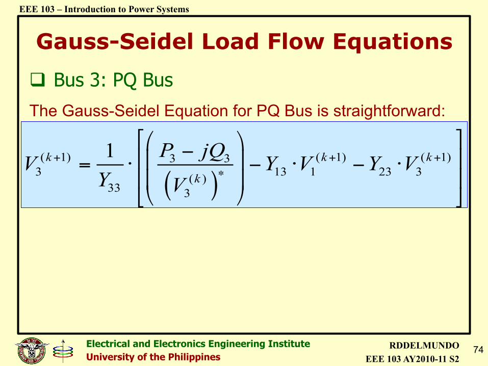
Gauss-Seidel Load Flow Equations
! Bus 3: PQ Bus
( )( 1) ( 1) ( 1)3 33 13 1 23 3( )
33 3
1k k k
k
P jQV Y V Y VY V
+ + +∗
" #$ %−' () *= ⋅ − ⋅ − ⋅' () *, -. /
The Gauss-Seidel Equation for PQ Bus is straightforward:
75 Electrical and Electronics Engineering Institute University of the Philippines
RDDELMUNDO EEE 103 AY2010-11 S2
EEE 103 – Introduction to Power Systems
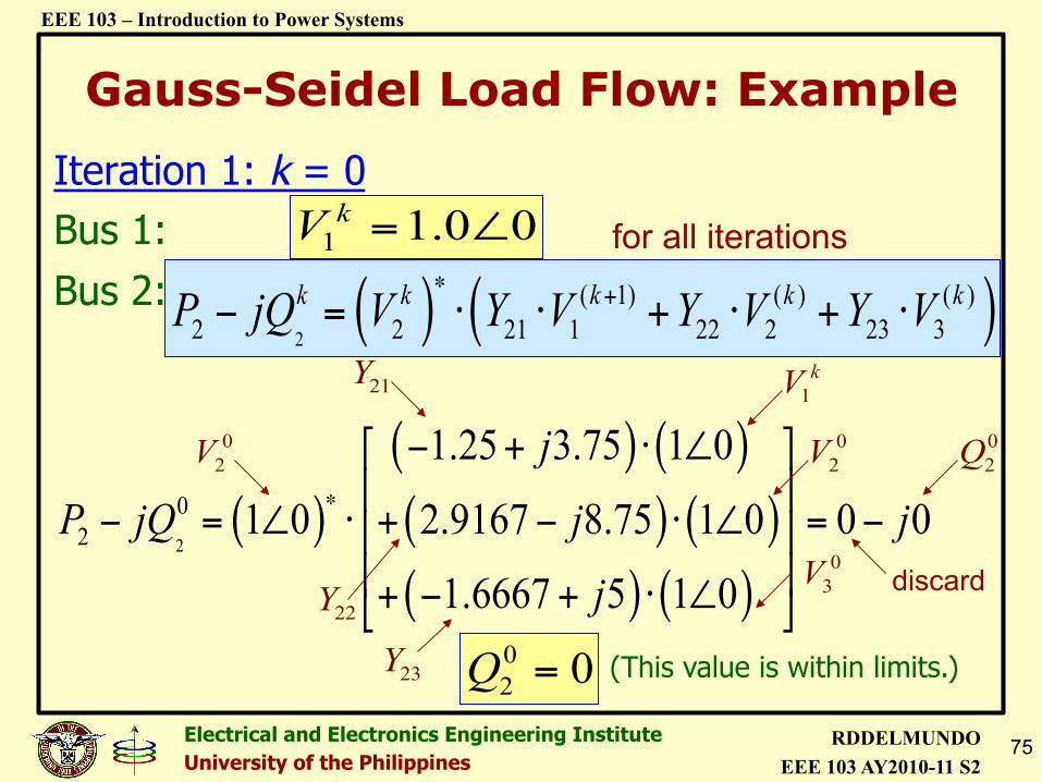
Gauss-Seidel Load Flow: Example Iteration 1: k = 0 Bus 1: Bus 2:
for all iterations 1 1.0 0kV = ∠
( ) ( )2
( 1) ( ) ( )2 2 21 1 22 2 23 3
k k k k kP jQ V Y V Y V Y V∗ +− = ⋅ ⋅ + ⋅ + ⋅
02 0Q =
( )( ) ( )( ) ( )( ) ( )
2
02
1.25 3.75 1 0
1 0 2.9167 8.75 1 0 0 0
1.6667 5 1 0
j
P jQ j j
j
∗
− + ⋅ ∠% &' (
− = ∠ ⋅ + − ⋅ ∠ = −' (' (+ − + ⋅ ∠) *
02V
21Y
22Y
23Y
1kV02V
03V discard
02Q
(This value is within limits.)
76 Electrical and Electronics Engineering Institute University of the Philippines
RDDELMUNDO EEE 103 AY2010-11 S2
EEE 103 – Introduction to Power Systems
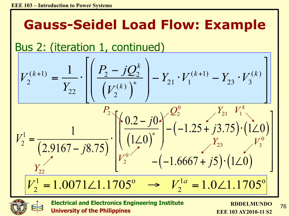
Gauss-Seidel Load Flow: Example Bus 2: (iteration 1, continued)
1 12 21.0071 1.1705 1.0 1.1705aV V= ∠ → = ∠o o
( ) ( )( ) ( )
( ) ( )
12
0.2 0 1.25 3.75 1 011 0
2.9167 8.751.6667 5 1 0
j jV
jj
∗
" #$ %−' (− − + ⋅ ∠+ ,+ ,= ⋅ ∠' (- .− ' (
− − + ⋅ ∠' (/ 0
( )( 1) ( 1) ( )2 22 21 1 23 3( )
22 2
1 kk k k
k
P jQV Y V Y VY V
+ +∗
" #$ %−' () *= ⋅ − ⋅ − ⋅' () *, -. /
22Y02V
2P 02Q 21Y 1
kV
23Y03V
77 Electrical and Electronics Engineering Institute University of the Philippines
RDDELMUNDO EEE 103 AY2010-11 S2
EEE 103 – Introduction to Power Systems
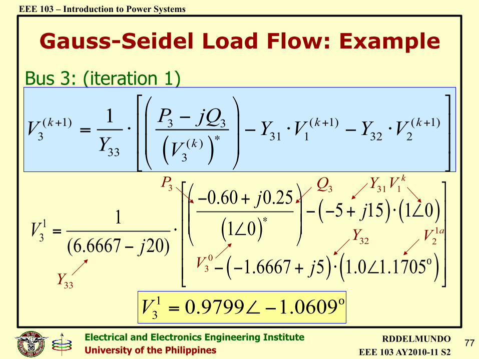
Gauss-Seidel Load Flow: Example Bus 3: (iteration 1)
13 0.9799 1.0609V = ∠− o
( )( ) ( )
( ) ( )
13
0.60 0.25 5 15 1 01 1 0(6.6667 20)
1.6667 5 1.0 1.1705
j jV
jj
∗
" #$ %− +' (− − + ⋅ ∠+ ,+ ,∠' (= ⋅ - .− ' (
− − + ⋅ ∠' (/ 0o
( )( 1) ( 1) ( 1)3 33 31 1 32 2( )
33 3
1k k k
k
P jQV Y V Y VY V
+ + +∗
" #$ %−' () *= ⋅ − ⋅ − ⋅' () *, -. /
33Y03V
3P 3Q 31Y 1kV
32Y12aV
78 Electrical and Electronics Engineering Institute University of the Philippines
RDDELMUNDO EEE 103 AY2010-11 S2
EEE 103 – Introduction to Power Systems
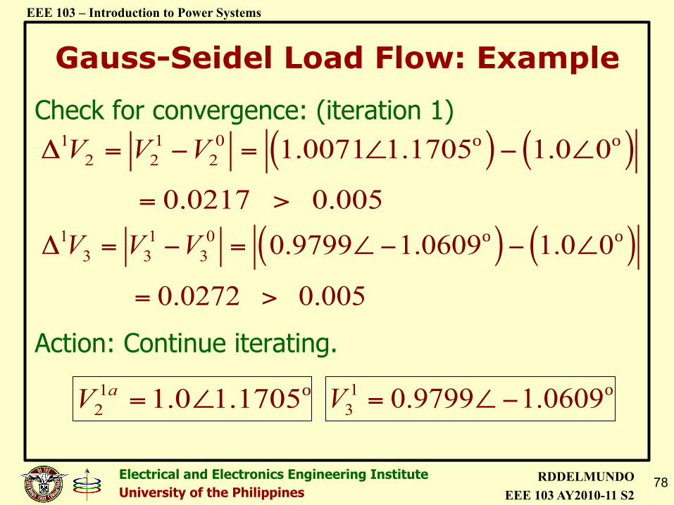
Gauss-Seidel Load Flow: Example Check for convergence: (iteration 1) Action: Continue iterating.
( ) ( )1 1 02 2 2 1.0071 1.1705 1.0 0
0.0217 0.005
V V VΔ = − = ∠ − ∠
= >
o o
( ) ( )1 1 03 3 3 0.9799 1.0609 1.0 0
0.0272 0.005
V V VΔ = − = ∠− − ∠
= >
o o
12 1.0 1.1705aV = ∠ o 1
3 0.9799 1.0609V = ∠− o
79 Electrical and Electronics Engineering Institute University of the Philippines
RDDELMUNDO EEE 103 AY2010-11 S2
EEE 103 – Introduction to Power Systems
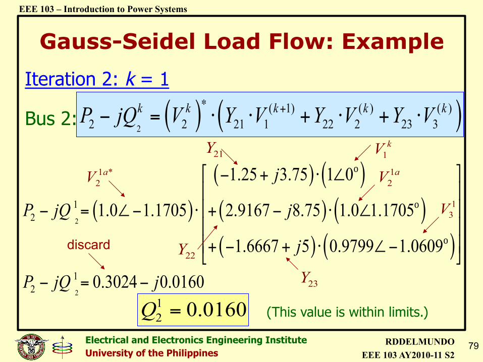
Gauss-Seidel Load Flow: Example Iteration 2: k = 1
Bus 2: ( ) ( )2
( 1) ( ) ( )2 2 21 1 22 2 23 3
k k k k kP jQ V Y V Y V Y V∗ +− = ⋅ ⋅ + ⋅ + ⋅
12 0.0160Q =
( )
( ) ( )( ) ( )( ) ( )
2
2
12
12
1.25 3.75 1 0
1.0 1.1705 2.9167 8.75 1.0 1.1705
1.6667 5 0.9799 1.0609
0.3024 0.0160
j
P jQ j
j
P jQ j
! "− + ⋅ ∠& '& '− = ∠− ⋅ + − ⋅ ∠& '& '+ − + ⋅ ∠−( )
− = −
o
o
o
1 *2aV
21Y
22Y
23Y
1kV12aV
13V
(This value is within limits.)
discard
80 Electrical and Electronics Engineering Institute University of the Philippines
RDDELMUNDO EEE 103 AY2010-11 S2
EEE 103 – Introduction to Power Systems
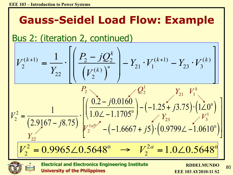
Gauss-Seidel Load Flow: Example Bus 2: (iteration 2, continued)
2 22 20.9965 0.5648 1.0 0.5648aV V= ∠ → = ∠o o
( )( ) ( )
( ) ( )22
0.2 0.0160 1.25 3.75 1 01 1.0 1.17052.9167 8.75
1.6667 5 0.9799 1.0610
j jV
jj
! − #$ % − − + ⋅ ∠( )* +∠−, -= ⋅ * +− * +− − + ⋅ ∠−. /
oo
o
( )( 1) ( 1) ( )2 22 21 1 23 3( )
22 2
1 kk k k
k
P jQV Y V Y VY V
+ +∗
" #$ %−' () *= ⋅ − ⋅ − ⋅' () *, -. /
22Y1 *2aV
2P 12Q 21Y 1
kV
23Y13V
81 Electrical and Electronics Engineering Institute University of the Philippines
RDDELMUNDO EEE 103 AY2010-11 S2
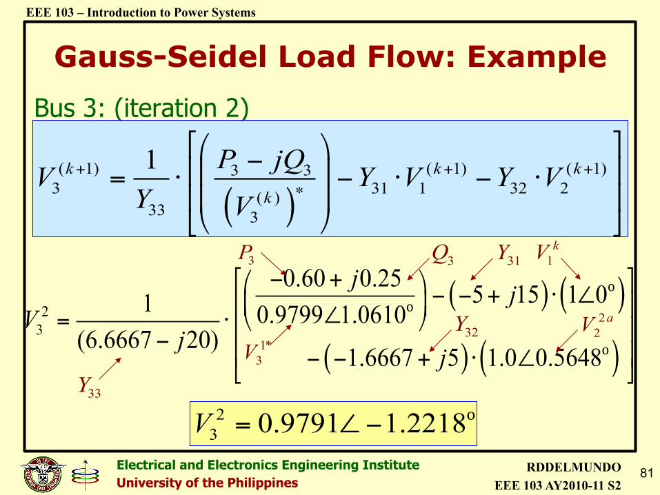
EEE 103 – Introduction to Power Systems
Gauss-Seidel Load Flow: Example Bus 3: (iteration 2)
23 0.9791 1.2218V = ∠− o
( ) ( )
( ) ( )23
0.60 0.25 5 15 1 01 0.9799 1.0610(6.6667 20)
1.6667 5 1.0 0.5648
j jV
jj
! − + #$ % − − + ⋅ ∠( )* +∠, -= ⋅ * +− * +− − + ⋅ ∠. /
oo
o
( )( 1) ( 1) ( 1)3 33 31 1 32 2( )
33 3
1k k k
k
P jQV Y V Y VY V
+ + +∗
" #$ %−' () *= ⋅ − ⋅ − ⋅' () *, -. /
33Y
1*3V
3P 3Q 31Y 1kV
32Y22aV
82 Electrical and Electronics Engineering Institute University of the Philippines
RDDELMUNDO EEE 103 AY2010-11 S2
EEE 103 – Introduction to Power Systems
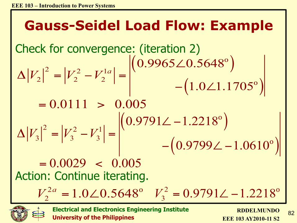
Gauss-Seidel Load Flow: Example Check for convergence: (iteration 2)
Action: Continue iterating.
( )( )
2 2 12 2 2
0.9965 0.5648
1.0 1.1705aV V V
∠Δ = − =
− ∠
o
o
( )( )
2 2 13 3 3
0.9791 1.2218
0.9799 1.0610V V V
∠−Δ = − =
− ∠−
o
o
22 1.0 0.5648aV = ∠ o 2
3 0.9791 1.2218V = ∠− o
0.0111 0.005= >
0.0029 0.005= <
83 Electrical and Electronics Engineering Institute University of the Philippines
RDDELMUNDO EEE 103 AY2010-11 S2
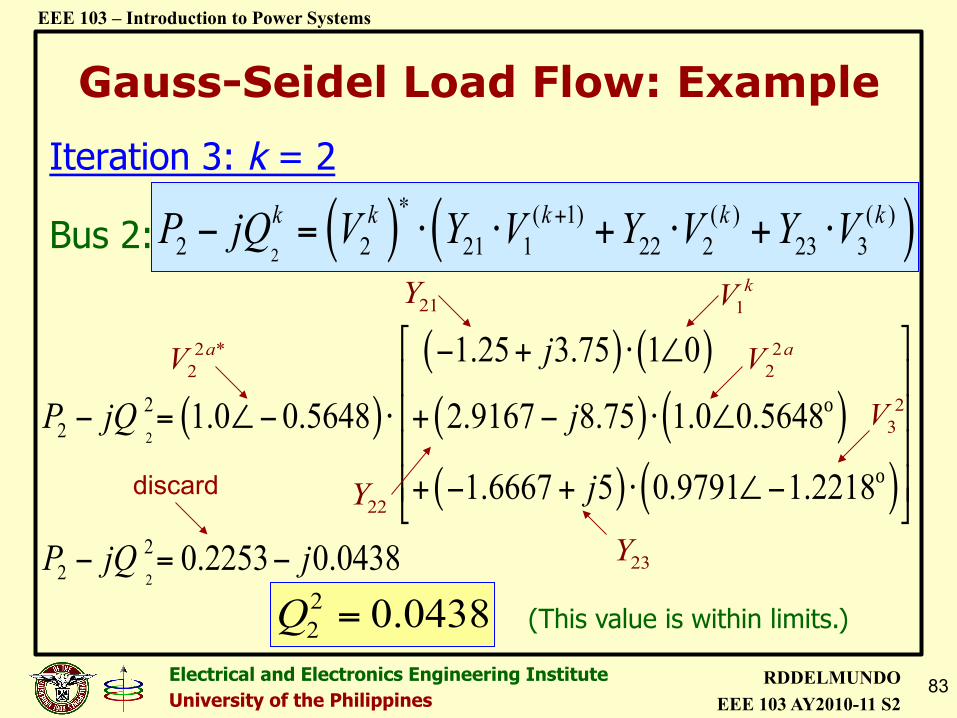
EEE 103 – Introduction to Power Systems
Gauss-Seidel Load Flow: Example Iteration 3: k = 2
Bus 2: ( ) ( )2
( 1) ( ) ( )2 2 21 1 22 2 23 3
k k k k kP jQ V Y V Y V Y V∗ +− = ⋅ ⋅ + ⋅ + ⋅
22 0.0438Q =
( )( ) ( )( ) ( )( ) ( )
2
2
22
22
1.25 3.75 1 0
1.0 0.5648 2.9167 8.75 1.0 0.5648
1.6667 5 0.9791 1.2218
0.2253 0.0438
j
P jQ j
j
P jQ j
! "− + ⋅ ∠& '& '− = ∠− ⋅ + − ⋅ ∠& '& '+ − + ⋅ ∠−( )
− = −
o
o
2 *2aV
21Y
22Y
23Y
1kV22aV
23V
(This value is within limits.)
discard
84 Electrical and Electronics Engineering Institute University of the Philippines
RDDELMUNDO EEE 103 AY2010-11 S2
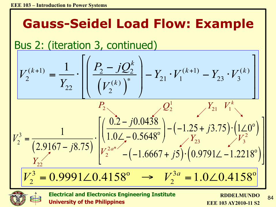
EEE 103 – Introduction to Power Systems
Gauss-Seidel Load Flow: Example Bus 2: (iteration 3, continued)
3 32 20.9991 0.4158 1.0 0.4158aV V= ∠ → = ∠o o
( )( ) ( )
( ) ( )32
0.2 0.0438 1.25 3.75 1 01 1.0 0.56482.9167 8.75
1.6667 5 0.9791 1.2218
j jV
jj
! − #$ % − − + ⋅ ∠( )* +∠−, -= ⋅ * +− * +− − + ⋅ ∠−. /
oo
o
( )( 1) ( 1) ( )2 22 21 1 23 3( )
22 2
1 kk k k
k
P jQV Y V Y VY V
+ +∗
" #$ %−' () *= ⋅ − ⋅ − ⋅' () *, -. /
22Y2 *2aV
2P 12Q 21Y 1
kV
23Y23V
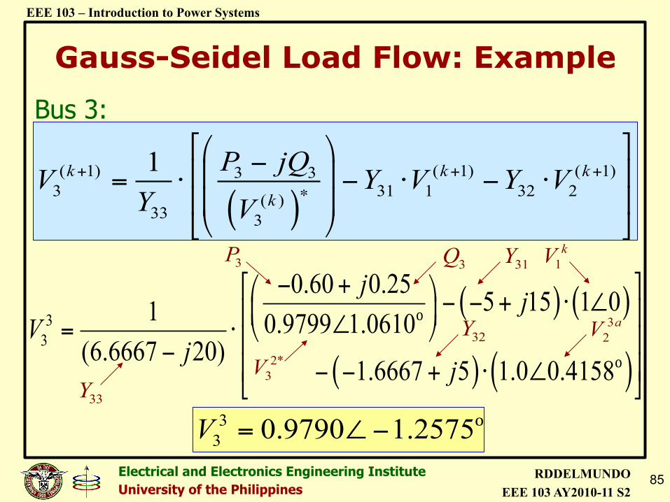
85 Electrical and Electronics Engineering Institute University of the Philippines
RDDELMUNDO EEE 103 AY2010-11 S2
EEE 103 – Introduction to Power Systems
Gauss-Seidel Load Flow: Example Bus 3:
33 0.9790 1.2575V = ∠− o
( ) ( )
( ) ( )33
0.60 0.25 5 15 1 01 0.9799 1.0610(6.6667 20)
1.6667 5 1.0 0.4158
j jV
jj
! − + #$ % − − + ⋅ ∠( )* +∠, -= ⋅ * +− * +− − + ⋅ ∠. /
o
o
( )( 1) ( 1) ( 1)3 33 31 1 32 2( )
33 3
1k k k
k
P jQV Y V Y VY V
+ + +∗
" #$ %−' () *= ⋅ − ⋅ − ⋅' () *, -. /
33Y2*3V
3P 3Q 31Y 1kV
32Y32aV
86 Electrical and Electronics Engineering Institute University of the Philippines
RDDELMUNDO EEE 103 AY2010-11 S2
EEE 103 – Introduction to Power Systems
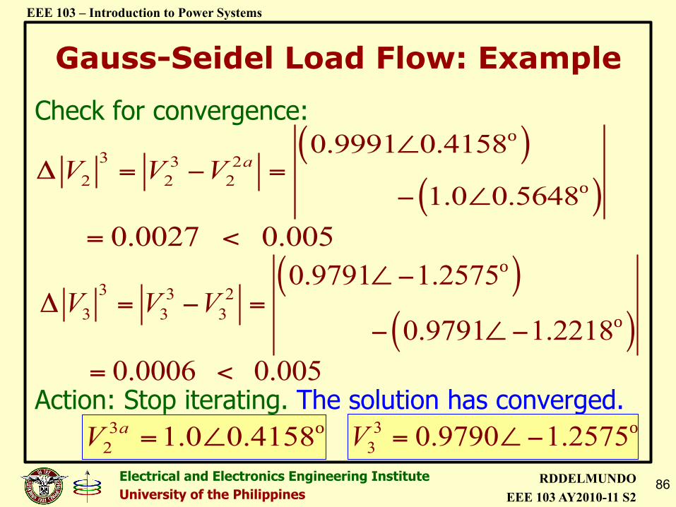
Gauss-Seidel Load Flow: Example Check for convergence:
Action: Stop iterating. The solution has converged.
( )( )
3 3 22 2 2
0.9991 0.4158
1.0 0.5648aV V V
∠Δ = − =
− ∠
o
o
( )( )
3 3 23 3 3
0.9791 1.2575
0.9791 1.2218V V V
∠−Δ = − =
− ∠−
o
o
32 1.0 0.4158aV = ∠ o 3
3 0.9790 1.2575V = ∠− o
0.0027 0.005= <
0.0006 0.005= <
88 Electrical and Electronics Engineering Institute University of the Philippines
RDDELMUNDO EEE 103 AY2010-11 S2
EEE 103 – Introduction to Power Systems
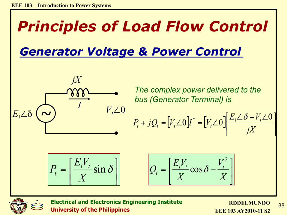
I
jX
Ei∠δ Vt∠0
Generator Voltage & Power Control
~
The complex power delivered to the bus (Generator Terminal) is
[ ] [ ] !"
#$%
& ∠−∠∠=∠=+
jXVEVIVjQP ti
tttt000 * δ
!"
#$%
&= δsinXVEP ti
t !"
#$%
&−=XV
XVEQ tti
t
2
cosδ
Principles of Load Flow Control
89 Electrical and Electronics Engineering Institute University of the Philippines
RDDELMUNDO EEE 103 AY2010-11 S2
EEE 103 – Introduction to Power Systems
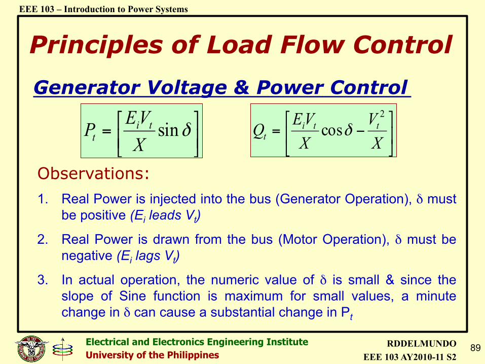
Generator Voltage & Power Control
!"
#$%
&= δsinXVEP ti
t !"
#$%
&−=XV
XVEQ tti
t
2
cosδ
Observations: 1. Real Power is injected into the bus (Generator Operation), δ must
be positive (Ei leads Vt)
2. Real Power is drawn from the bus (Motor Operation), δ must be negative (Ei lags Vt)
3. In actual operation, the numeric value of δ is small & since the slope of Sine function is maximum for small values, a minute change in δ can cause a substantial change in Pt
Principles of Load Flow Control
90 Electrical and Electronics Engineering Institute University of the Philippines
RDDELMUNDO EEE 103 AY2010-11 S2
EEE 103 – Introduction to Power Systems
Generator Voltage & Power Control
!"
#$%
&= δsinXVEP ti
t !"
#$%
&−=XV
XVEQ tti
t
2
cosδ
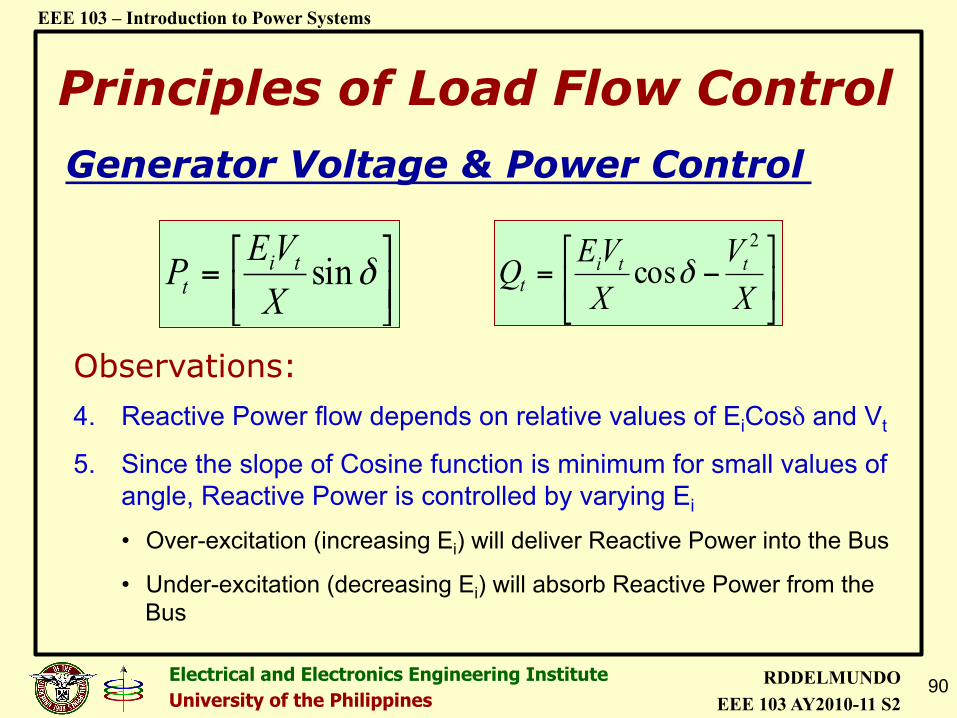
Observations: 4. Reactive Power flow depends on relative values of EiCosδ and Vt
5. Since the slope of Cosine function is minimum for small values of angle, Reactive Power is controlled by varying Ei • Over-excitation (increasing Ei) will deliver Reactive Power into the Bus
• Under-excitation (decreasing Ei) will absorb Reactive Power from the Bus
Principles of Load Flow Control
91 Electrical and Electronics Engineering Institute University of the Philippines
RDDELMUNDO EEE 103 AY2010-11 S2
EEE 103 – Introduction to Power Systems
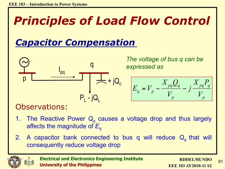
Capacitor Compensation
Ipq p
q
PL - jQL
+ jQc
~
p
qpq
p
qpqpq V
PXj
VQX
VE −−=
The voltage of bus q can be expressed as
Observations: 1. The Reactive Power Qq causes a voltage drop and thus largely
affects the magnitude of Eq
2. A capacitor bank connected to bus q will reduce Qq that will consequently reduce voltage drop
Principles of Load Flow Control
92 Electrical and Electronics Engineering Institute University of the Philippines
RDDELMUNDO EEE 103 AY2010-11 S2
EEE 103 – Introduction to Power Systems
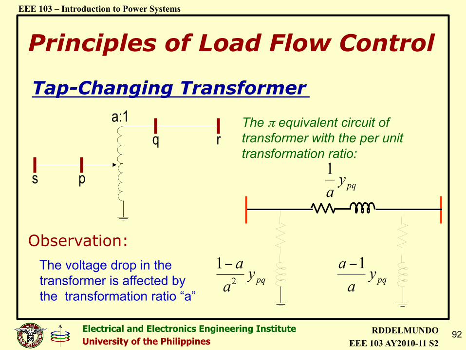
Tap-Changing Transformer a:1
q r
s p
The π equivalent circuit of transformer with the per unit transformation ratio:
pqyaa2
1−pqya
a 1−
pqya1
Observation: The voltage drop in the transformer is affected by the transformation ratio “a”
Principles of Load Flow Control
94 Electrical and Electronics Engineering Institute University of the Philippines
RDDELMUNDO EEE 103 AY2010-11 S2
EEE 103 – Introduction to Power Systems
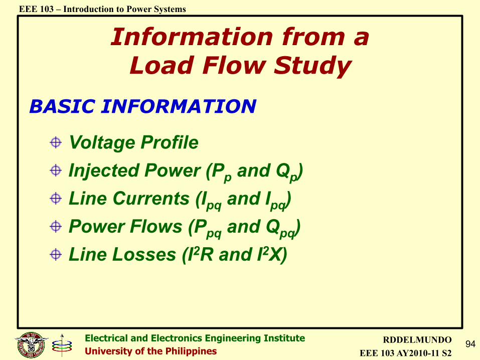
BASIC INFORMATION
" Voltage Profile " Injected Power (Pp and Qp) " Line Currents (Ipq and Ipq) " Power Flows (Ppq and Qpq) " Line Losses (I2R and I2X)
Information from a Load Flow Study
95 Electrical and Electronics Engineering Institute University of the Philippines
RDDELMUNDO EEE 103 AY2010-11 S2
EEE 103 – Introduction to Power Systems
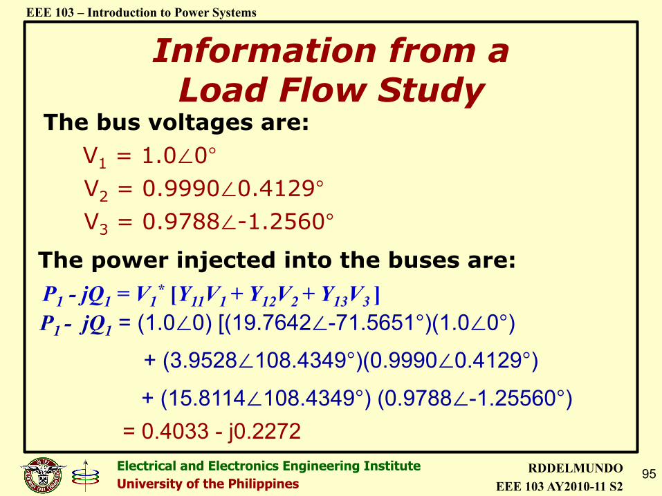
The bus voltages are: V1 = 1.0∠0° V2 = 0.9990∠0.4129° V3 = 0.9788∠-1.2560°
The power injected into the buses are:
P1 - jQ1 = (1.0∠0) [(19.7642∠-71.5651°)(1.0∠0°)
+ (3.9528∠108.4349°)(0.9990∠0.4129°)
+ (15.8114∠108.4349°) (0.9788∠-1.25560°) = 0.4033 - j0.2272
P1 - jQ1 = V1* [Y11V1 + Y12V2 + Y13V3 ]
Information from a Load Flow Study
96 Electrical and Electronics Engineering Institute University of the Philippines
RDDELMUNDO EEE 103 AY2010-11 S2
EEE 103 – Introduction to Power Systems
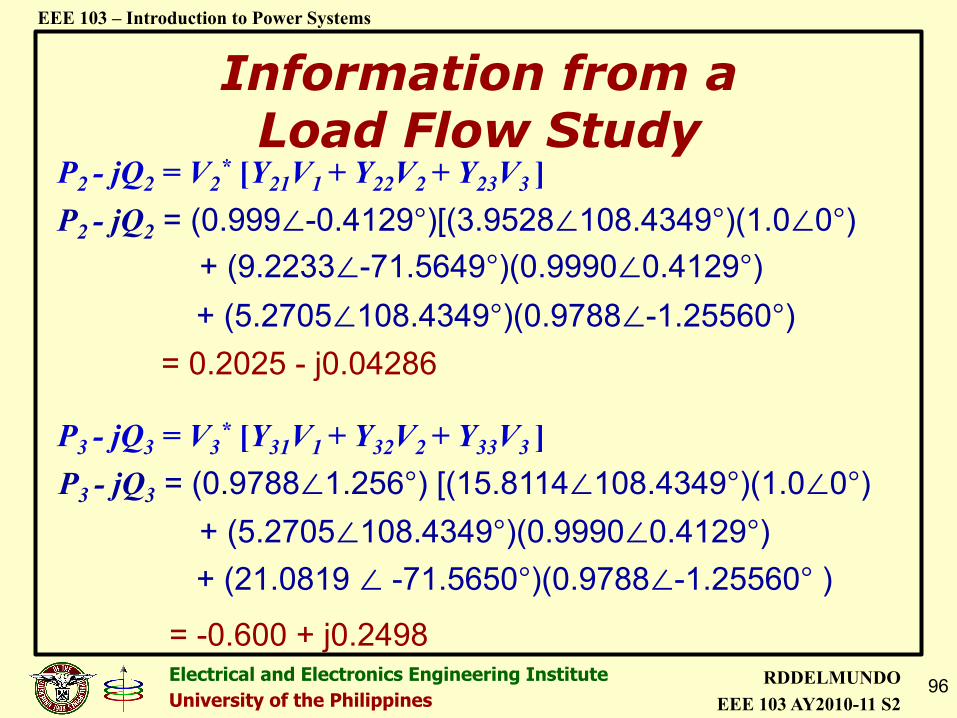
P2 - jQ2 = (0.999∠-0.4129°)[(3.9528∠108.4349°)(1.0∠0°) + (9.2233∠-71.5649°)(0.9990∠0.4129°) + (5.2705∠108.4349°)(0.9788∠-1.25560°)
= 0.2025 - j0.04286
P3 - jQ3 = (0.9788∠1.256°) [(15.8114∠108.4349°)(1.0∠0°) + (5.2705∠108.4349°)(0.9990∠0.4129°) + (21.0819 ∠ -71.5650°)(0.9788∠-1.25560° )
= -0.600 + j0.2498
P2 - jQ2 = V2* [Y21V1 + Y22V2 + Y23V3 ]
P3 - jQ3 = V3* [Y31V1 + Y32V2 + Y33V3 ]
Information from a Load Flow Study
97 Electrical and Electronics Engineering Institute University of the Philippines
RDDELMUNDO EEE 103 AY2010-11 S2
EEE 103 – Introduction to Power Systems
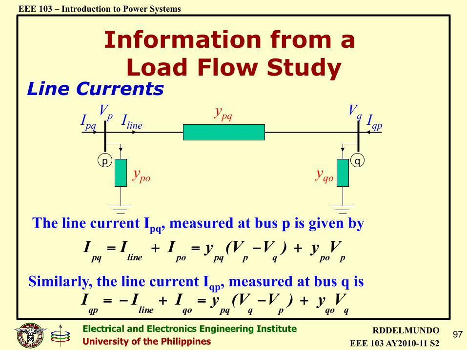
p q ypo yqo
ypq Ipq Iqp Iline Vp Vq
ppoqppqpolinepqVy )VV(yI II +−=+=
qqopqpqqolineqpVy )VV(yI I I +−=+−=
The line current Ipq, measured at bus p is given by
Similarly, the line current Iqp, measured at bus q is
Line Currents
Information from a Load Flow Study
98 Electrical and Electronics Engineering Institute University of the Philippines
RDDELMUNDO EEE 103 AY2010-11 S2
EEE 103 – Introduction to Power Systems
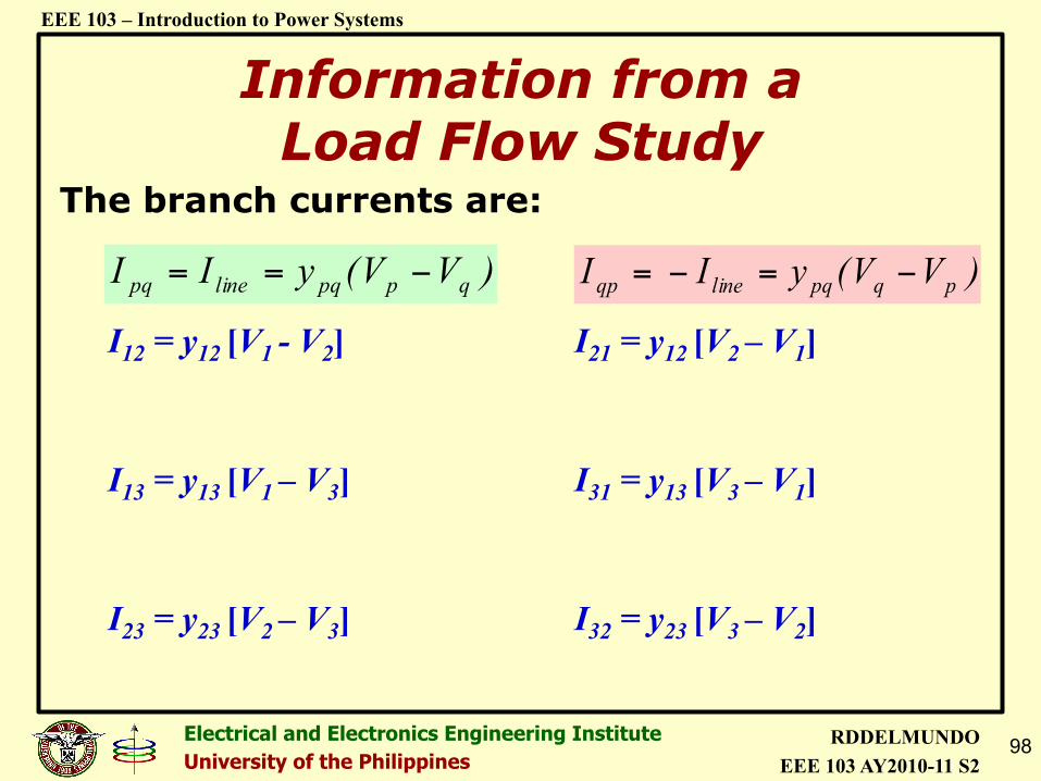
The branch currents are:
)VV(yII qppqlinepq −== )VV(yI I pqpqlineqp −=−=
I12 = y12 [V1 - V2] I21 = y12 [V2 – V1]
I13 = y13 [V1 – V3] I31 = y13 [V3 – V1]
I23 = y23 [V2 – V3] I32 = y23 [V3 – V2]
Information from a Load Flow Study
99 Electrical and Electronics Engineering Institute University of the Philippines
RDDELMUNDO EEE 103 AY2010-11 S2
EEE 103 – Introduction to Power Systems
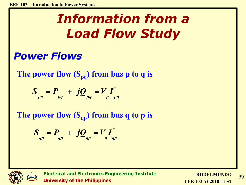
The power flow (Spq) from bus p to q is *
pqppqpqpqIVQj PS =+=
The power flow (Sqp) from bus q to p is *
qpqqpqpqpIVQj PS =+=
Power Flows
Information from a Load Flow Study
100 Electrical and Electronics Engineering Institute University of the Philippines
RDDELMUNDO EEE 103 AY2010-11 S2
EEE 103 – Introduction to Power Systems
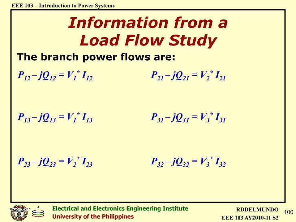
The branch power flows are:
P12 – jQ12 = V1* I12 P21 – jQ21 = V2
* I21
P13 – jQ13 = V1* I13 P31 – jQ31 = V3
* I31
P23 – jQ23 = V2* I23 P32 – jQ32 = V3
* I32
Information from a Load Flow Study
101 Electrical and Electronics Engineering Institute University of the Philippines
RDDELMUNDO EEE 103 AY2010-11 S2
EEE 103 – Introduction to Power Systems
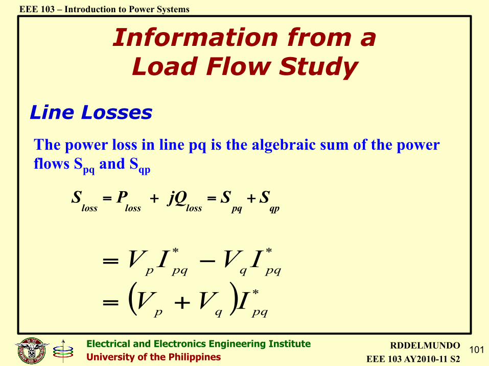
The power loss in line pq is the algebraic sum of the power flows Spq and Sqp
qppqlosslosslossSSQj PS +=+=
Line Losses
Information from a Load Flow Study
( ) *pqqp
*pqq
*pqp
IVVIVIV
+=
−=
102 Electrical and Electronics Engineering Institute University of the Philippines
RDDELMUNDO EEE 103 AY2010-11 S2
EEE 103 – Introduction to Power Systems
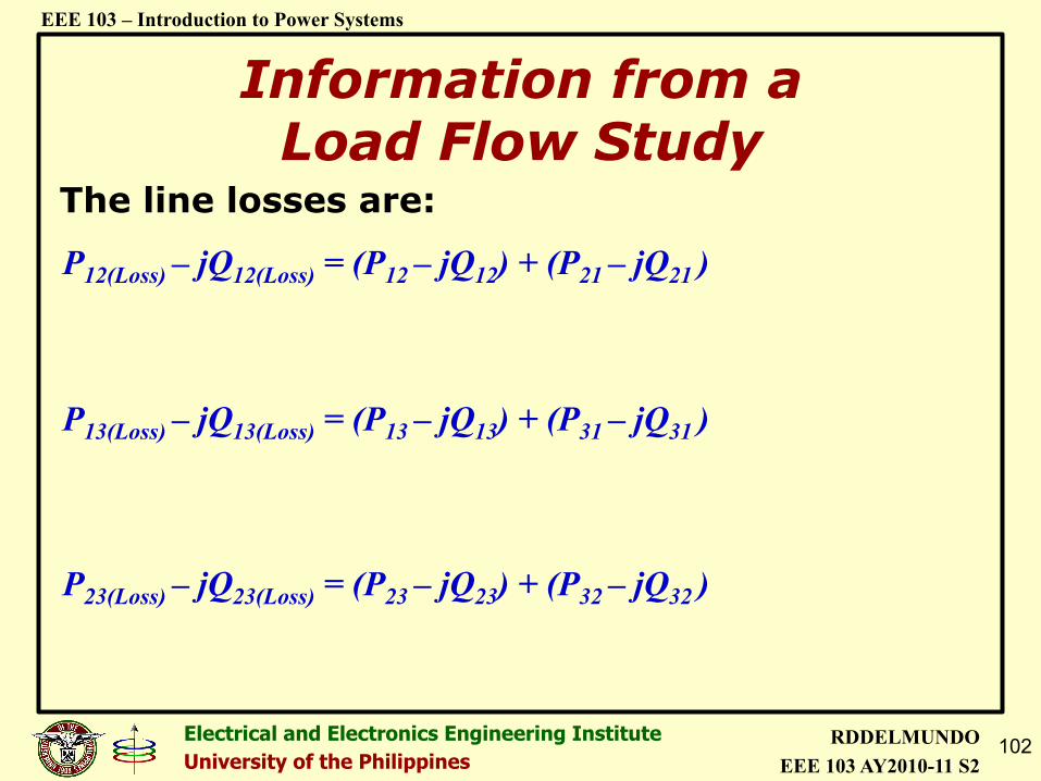
The line losses are:
P12(Loss) – jQ12(Loss) = (P12 – jQ12) + (P21 – jQ21 )
P13(Loss) – jQ13(Loss) = (P13 – jQ13) + (P31 – jQ31 )
P23(Loss) – jQ23(Loss) = (P23 – jQ23) + (P32 – jQ32 )
Information from a Load Flow Study
103 Electrical and Electronics Engineering Institute University of the Philippines
RDDELMUNDO EEE 103 AY2010-11 S2
EEE 103 – Introduction to Power Systems
Information from a Load Flow Study
Other Information:
" Overvoltage and Undervoltage Buses " Critical and Overloaded Transformers
and Lines " Total System Losses
105 Electrical and Electronics Engineering Institute University of the Philippines
RDDELMUNDO EEE 103 AY2010-11 S2
EEE 103 – Introduction to Power Systems
Sensitivity Analysis with Load Flow Study
9) Add or remove rotating or static var supply to buses.
8) Increase or decrease transformer size.
7) Change transformer taps.
6) Change bus voltages.
5) Increase conductor size on T&D lines.
4) Add new transmission or distribution lines.
3) Add, remove or shift generation to any bus.
2) Add, reduce or remove load to any or all buses. 1) Take any line, transformer or generator out of service.
Uses of Load Flow Studies

106 Electrical and Electronics Engineering Institute University of the Philippines
RDDELMUNDO EEE 103 AY2010-11 S2
EEE 103 – Introduction to Power Systems
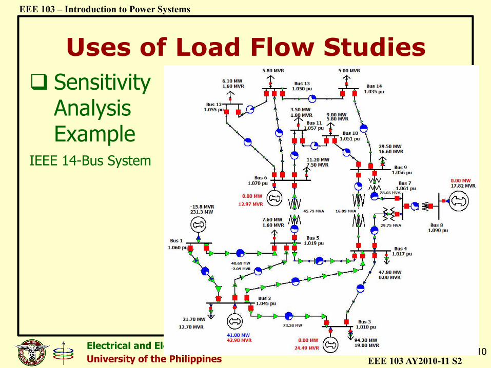
Uses of Load Flow Studies ! Sensitivity
Analysis Example
IEEE 14-Bus System
107 Electrical and Electronics Engineering Institute University of the Philippines
RDDELMUNDO EEE 103 AY2010-11 S2
EEE 103 – Introduction to Power Systems
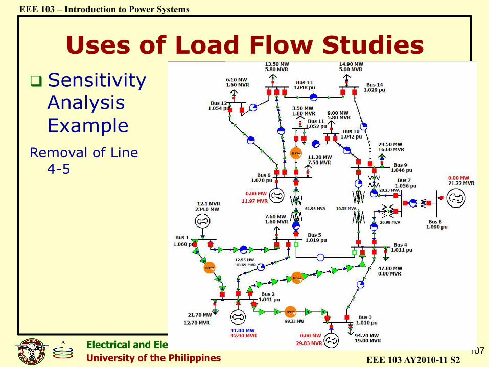
Uses of Load Flow Studies ! Sensitivity
Analysis Example
Removal of Line 4-5

108 Electrical and Electronics Engineering Institute University of the Philippines
RDDELMUNDO EEE 103 AY2010-11 S2
EEE 103 – Introduction to Power Systems
Uses of Load Flow Studies ! Sensitivity
Analysis Example
IEEE 14-Bus System
109 Electrical and Electronics Engineering Institute University of the Philippines
RDDELMUNDO EEE 103 AY2010-11 S2
EEE 103 – Introduction to Power Systems
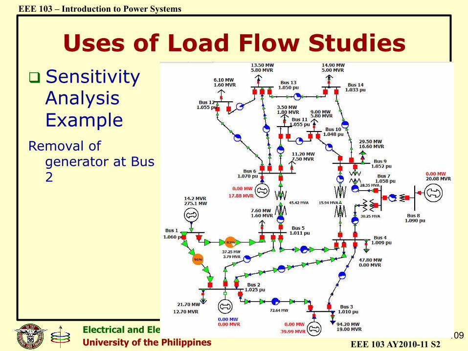
Uses of Load Flow Studies ! Sensitivity
Analysis Example
Removal of generator at Bus 2
110 Electrical and Electronics Engineering Institute University of the Philippines
RDDELMUNDO EEE 103 AY2010-11 S2
EEE 103 – Introduction to Power Systems
Uses of Load Flow Studies ! Sensitivity
Analysis Example
IEEE 14-Bus System
111 Electrical and Electronics Engineering Institute University of the Philippines
RDDELMUNDO EEE 103 AY2010-11 S2
EEE 103 – Introduction to Power Systems
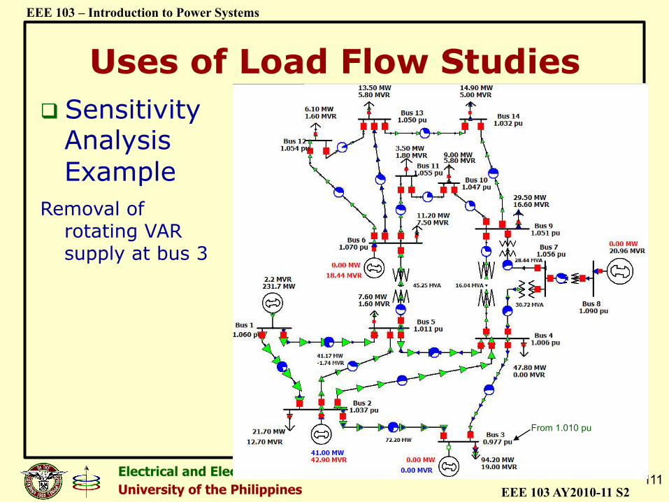
Uses of Load Flow Studies ! Sensitivity
Analysis Example
Removal of rotating VAR supply at bus 3
From 1.010 pu

112 Electrical and Electronics Engineering Institute University of the Philippines
RDDELMUNDO EEE 103 AY2010-11 S2
EEE 103 – Introduction to Power Systems
Uses of Load Flow Studies ! Sensitivity
Analysis Example
IEEE 14-Bus System
113 Electrical and Electronics Engineering Institute University of the Philippines
RDDELMUNDO EEE 103 AY2010-11 S2
EEE 103 – Introduction to Power Systems
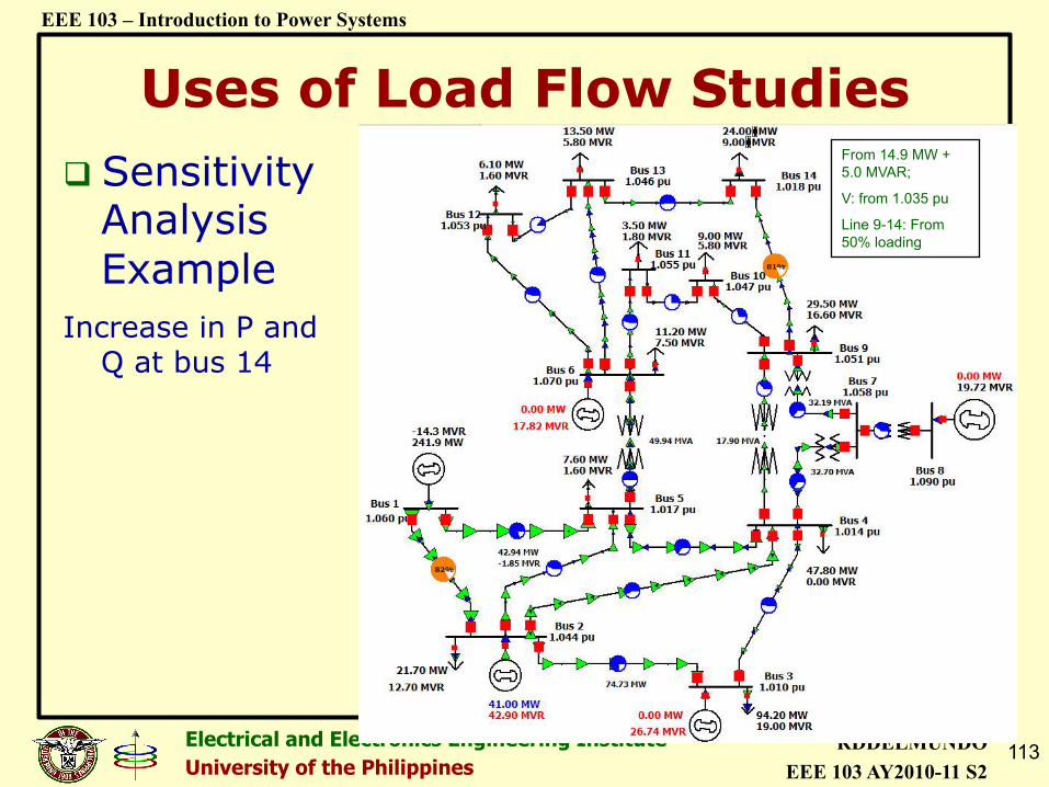
Uses of Load Flow Studies ! Sensitivity
Analysis Example
Increase in P and Q at bus 14
From 14.9 MW + 5.0 MVAR;
V: from 1.035 pu
Line 9-14: From 50% loading
114 Electrical and Electronics Engineering Institute University of the Philippines
RDDELMUNDO EEE 103 AY2010-11 S2
EEE 103 – Introduction to Power Systems
Uses of Load Flow Studies
! Analysis of existing conditions: ! Check for voltage violations (undervoltage/overvoltage). ! Check for transformer overloading/line overloading. ! Check for system losses.
! Analysis for correction of power quality issues: ! Voltage adjustment at the delivery points ! Transformer tap changing ! Capacitor compensation:
" Compensation for Peak Loading " Check for overvoltages during Off-Peak conditions " Optimize capacitor allocation and capacitor switching
115 Electrical and Electronics Engineering Institute University of the Philippines
RDDELMUNDO EEE 103 AY2010-11 S2
EEE 103 – Introduction to Power Systems
Uses of Load Flow Studies
! Analysis for Expansion Planning: ! Construction of new substation ! Addition of capacity to existing substation ! Construction of new feeder segment ! Extension of existing feeder segment ! Addition of parallel feeder segment ! Replacement of conductors in existing feeder segments ! Conversion of entire feeder circuits from one voltage
level to another voltage level ! Addition of generators
116 Electrical and Electronics Engineering Institute University of the Philippines
RDDELMUNDO EEE 103 AY2010-11 S2
EEE 103 – Introduction to Power Systems
Uses of Load Flow Studies
! Contingency Analysis: ! Reliability of the Transmission, Subtransmission, and
Distribution Systems Reliability denotes that not only is the power system working, but that it is working properly. That is, no physical and technical constraints must be violated – i.e., voltage must be well regulated and within acceptable range, load limits of the transformers and the lines must not be exceeded, and power balance must be satisfied.
! System Loss Analysis: ! Identification of lossy components in the power system.