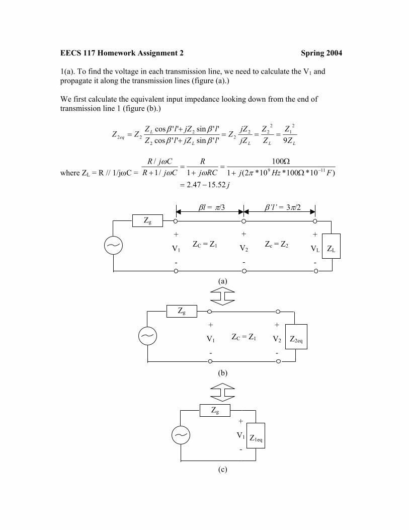
EECS 117 Homework Assignment 2 Spring 2004 1(a). To find the voltage in each transmission line, we need to calculate the V1 and propagate it along the transmission lines (figure (a).) We first calculate the equivalent input impedance looking down from the end of transmission line 1 (figure (b).)

LLLL

Leq Z

ZZZ

jZjZZ

ljZlZljZlZZZ

9''sin''cos''sin''cos 2

12

222

2

222 ===

++

=ββββ

where ZL = R // 1/jωC = j

FHzjRCjR

CjRCjR

52.1547.2)10*100*10*2(1

1001/1

/119

−=Ω+

Ω=

+=

+ −πωωω

β’l’ = 3π/2 βl = π/3

+

V1

-

Zc = Z2 +

VL

-

ZC = Z1 +

V2

-

ZL

Zg (a)

+

V2

-

+

V1

-

ZC = Z1

Z2eq

Zg (b)

+

V1

-

Z1eq

Zg

(c)

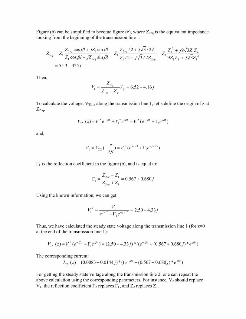
Figure (b) can be simplified to become figure (c), where Z1eq is the equivalent impedance looking from the beginning of the transmission line 1.

j

ZjZZZZjZZ

ZjZ

ZjZZ

ljZlZljZlZ

ZZL

L

eq

eq

eq

eqeq

4253.55

3939

2/32/

2/32/sincossincos

211

12

11

21

121

21

1211

−=

+

+=

+

+=

+

+=

ββββ

Then,

jVZZ

ZV g

geq

eq 16.452.61

11 −=

+=

To calculate the voltage, VTL1, along the transmission line 1, let’s define the origin of z at Z2eq.

)()( 11111zjzjzjzj

TL eeVeVeVzV ββββ Γ+=+= −+−−+ and,

)()3

( 3/1

3/111

ππ

βπ jj

TL eeVVV −+ Γ+=−=

Γ1 is the reflection coefficient in the figure (b), and is equal to:

jZZZZ

eq

eq 680.0567.012

121 +=

+

−=Γ

Using the known information, we can get

jee

VV jj 33.450.23/1

3/1

1 −=Γ+

= −+

ππ

Thus, we have calculated the steady state voltage along the transmission line 1 (for z=0 at the end of the transmission line 1):

)*)680.0567.0(((*)33.450.2()()( 111zjzjzjzj

TL ejejeeVzV ββββ ++−=Γ+= −−+

The corresponding current: )*)680.0567.0(((*)0144.00083.0()(1

zjzjTL ejejzI ββ +−−= −

For getting the steady state voltage along the transmission line 2, one can repeat the above calculation using the corresponding parameters. For instance, V2 should replace V1, the reflection coefficient Γ2 replaces Γ1, and Z2 replaces Z1.

jVVV TL 09.586.6)1()0( 112 −=Γ+== +

jZZZZ

L

L 289.0908.02

22 −−=

+−

=Γ

jee

VV jj 12.314.32/32

2/32

2 +=Γ+

= −+

ππ

For z’ = 0 at the load,

)*)289.0908.0(((*)12.314.3()()'( '''2

'22

zjzjzjzjTL ejejeeVzV ββββ +−+=Γ+= −−+

)*)289.0908.0(((*)0312.00314.0()'( ''

2zjzj

TL ejejzI ββ +++= −

(b) For line 1, 4.1611

1

1 =Γ−

Γ+=VSWR

For line 2, 5.4111

2

2 =Γ−

Γ+=VSWR

(c). The average power delivered to the load = [ ] *, Re

21

LLLav IVP = , where VL and IL are

the voltage and current at the load, respectively.

[ ] [ ] === 9)0()0(Re

21Re

21 *

22*

, TLTLLLLav IVIVP mW

(d). The average power delivered by the source to the transmission lines =

[ ]

=

=

== 91Re

2Re

21Re

21

1

21

*

1

11

*11,

eqeqLav Z

VZV

VIVP mW.

This is the same as the one in part (c), which is expected as the transmission lines are lossless. 2. (Two typos in the question: … desired to deliver 10W into ZL2 and the remaining power into ZL3.)

Since VSWR = 0 dB is required for each line and 11

+−

=ΓVSWRVSWR , |Γ| = 0. Thus, ZL2=Z2,

ZL3=Z3.

Because it is a perfect match, the length of the transmission lines does not change the impedance of the transmission lines seen from the junction downwards. The voltages at the junction of the two transmission lines are the same, for they are measured at the same junction. Thus, the currents going into individual lines determine the amount of power flowing into the respective loads.

( ) ( ) 4

1/1Re2/

/1Re2/

2

3

32

1

22

1

3

2 ===ZZ

ZV

ZVPP

L

L

So Z2 = 4 Z3 would make 10 W going into ZL2 and 40 W into ZL3.

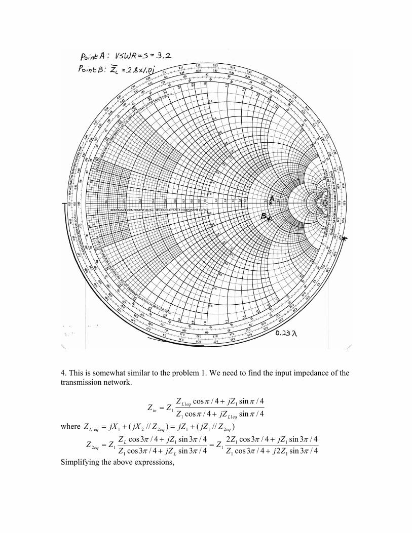
3. Given VWSR = 3.2, 524.011

=+−

=ΓVSWRVSWR

At the position in the transmission line where the voltage is minimum, the current is maximum, so the impedance and the impedance normalized to Z0 at that point is minimum. The impedance is also real. Thus the normalized impedance of this position has a point lying on the left hand part along the horizontal axis in the Smith chart. Since this position is 0.23 wavelength away from the load, you need to move the point counterclockwise 0.23λ to find the normalized impedance of the load. The new point has an angle subtended at the origin of -14.40. To find the distance of the new point from the origin of the chart, one needs to make use of the fact that propagation along the transmission line just rotates the impedance point about the origin. The radius of the circular locus does not change. At the position of the line where the voltage is maximum, the normalized impedance is maximum and real, and is equal to VWSR = 3.2. Thus, the point corresponding to the normalized load impedance can be obtained by moving this point about the origin of the chart, by –14.40. This point has a reading of 2.8 – 1.0j. Therefore, the load impedance is 196 – 70j Ω.

4. This is somewhat similar to the problem 1. We need to find the input impedance of the transmission network.

4/sin4/cos4/sin4/cos

11

111 ππ

ππ

eqL

eqLin jZZ

jZZZZ

+

+=

where )//()//( 2112211 eqeqeqL ZjZjZZjXjXZ +=+=

4/3sin24/3cos4/3sin4/3cos2

4/3sin4/3cos4/3sin4/3cos

11

111

1

112 ππ

ππππππ

ZjZjZZZ

jZZjZZZZ

L

Leq +

+=

++

=

Simplifying the above expressions,

12 )6.08.0( ZjZ eq +=

111

1111 )5.125.0(

)6.08.0()6.08.0(* ZjjZjZjZjZjZZ eqL +=

+++

+=

111

111 )2.46.1(

4/sin)5.125.0(4/cos4/sin4/cos)5.125.0( Zj

ZjjZjZZjZZin −=

++++

=ππππ

Thus, voltage across the beginning of the line 1, V1 is equal to:

jVZZ

ZV g

gin

in 861.047.41 −=+

=

Since the transmission lines are lossless, the power delivered into the line is equal to the power consumed by the load. Hence, power transmitted to the load =

11

21

*

1

11,

820.01Re2

Re21

ZZV

ZVVP

eqeqLav =

=

= W

Γ1 for transmission line 1 = jjj 787.0344.0

)15.125.0()15.125.0(

+=++−+

2.1311

1

1 =Γ−

Γ+=VSWR

Γ2 for transmission line 2 = 3/1)12()12(

=+−

211

2

2 =Γ−

Γ+=VSWR

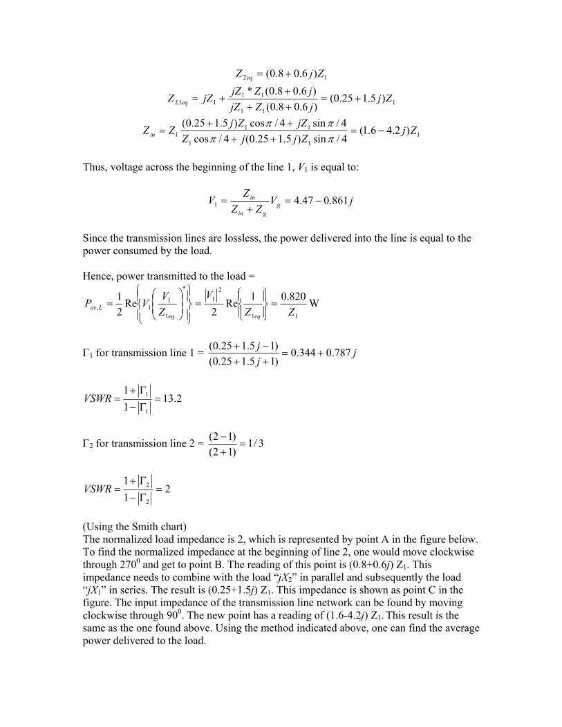
(Using the Smith chart) The normalized load impedance is 2, which is represented by point A in the figure below. To find the normalized impedance at the beginning of line 2, one would move clockwise through 2700 and get to point B. The reading of this point is (0.8+0.6j) Z1. This impedance needs to combine with the load “jX2” in parallel and subsequently the load “jX1” in series. The result is (0.25+1.5j) Z1. This impedance is shown as point C in the figure. The input impedance of the transmission line network can be found by moving clockwise through 900. The new point has a reading of (1.6-4.2j) Z1. This result is the same as the one found above. Using the method indicated above, one can find the average power delivered to the load.

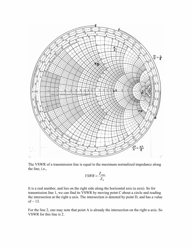
The VSWR of a transmission line is equal to the maximum normalized impedance along the line, i.e.,

0

max

ZZ

VSWR =

It is a real number, and lies on the right side along the horizontal axis (u axis). So for transmission line 1, we can find its VSWR by moving point C about a circle and reading the intersection at the right u axis. The intersection is denoted by point D, and has a value of ~ 13. For the line 2, one may note that point A is already the intersection on the right u axis. So VSWR for this line is 2.

5(a). In general, voltage and current along a transmission line have forms:

zz eVeVzV γγ −−+ +=)(

[ ]zz eVeVZ

zI γγ −−+ −=0

1)(

where ZY=γ

YZZ =0

'','' CjGYLjRZ ωω +=+= In this case, because R’>>ωL’, Z ~ R’. Y ~ j ωC’. Thus, the propagation constant

)1(2/'''' jCRCRj +== ωωγ . Since βαγ j+= , 2/''CRωβ = , and propagation

velocity = )''/(2/ CRωβω = . (b) Using the voltage and current expression given above, the input impedance is equal to be (z = -l) :

lZlZlZlZ

ZeeZ

eVeVeVeVZlZ

L

Ll

l

ll

ll

i γγγγ

γ

γ

γγ

γγ

sinhcoshsinhcosh

11)(

0

002

2

00 ++

=Γ−Γ+

=−+

= −

−

−−+

−−+

where ZL is the load impedance, )1()'2/(')'/('0 jCRCjRZ −== ωω , and l is the distance of the point of interest to the load. (c) For a shorted termination,

( ) ( )

+−==

++

= ljCRjC

RlZlZlZlZlZ

ZlZL

Li 1

2''tanh1

'2'tanh

sinhcoshsinhcosh

)( 00

00

ωω

γγγγγ

Expansion of Z0 around ω = 0 gives:

)(''

0 ωω

OC

jRZ +−=

O(ω) represents the higher-order terms in the expansion. Expansion of tanh(γl) around ω = 0 gives:

( ) )(''31''tanh 2/33 ωωωγ OlCjRjRClCRjl +−=

So,

CRjRZi2

31~ ω−

R and C are the sums of the resistance and capacitance of the components in the transmission model. At low frequency, the shorted transmission line acts like a resistor. This is true until the frequency is so large that the imaginary part, which is the reactive component of the impedance, is comparable to the real part. In particular, the parts become equal when

RCCRR

/3or 3/2

==

ωω

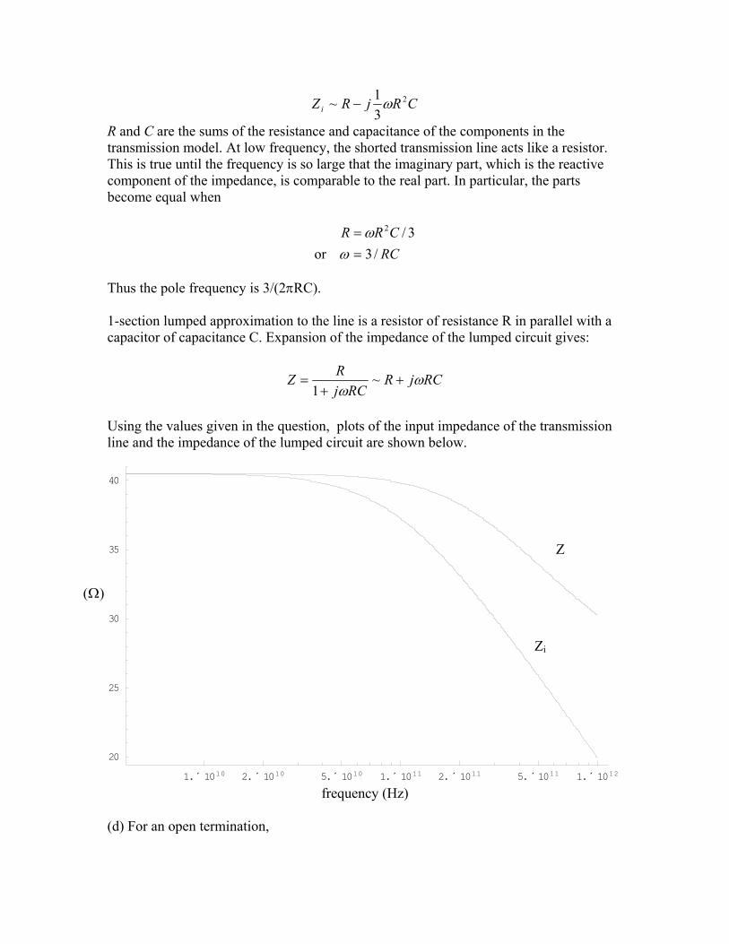
Thus the pole frequency is 3/(2πRC). 1-section lumped approximation to the line is a resistor of resistance R in parallel with a capacitor of capacitance C. Expansion of the impedance of the lumped circuit gives:

RCjRRCj

RZ ωω

++

= ~1

Using the values given in the question, plots of the input impedance of the transmission line and the impedance of the lumped circuit are shown below.

1. ´ 1010 2. ´ 1010 5. ´ 1010 1. ´ 1011 2. ´ 1011 5. ´ 1011 1. ´ 1012

20

25

30

35

40

Z

(Ω)

Zi

frequency (Hz) (d) For an open termination,

( ) ( )

+−==

++

= ljCRjC

RlZlZlZlZlZ

ZlZL

Li 1

2''tanh1

'2'tanh

sinhcoshsinhcosh

)( 00

00

ωω

γγγγγ

Just like in part (c), expansion of Z0 around ω = 0 gives:

)(''

0 ωω

OC

jRZ +−=

Expansion of 1/tanh(γl) around ω = 0 gives:

( ) ( ) )(45

''''3''

1tanh1 32

3

ωωωω

γ Olj

CRljCRj

lCRjl +++=

Combining the two results gives:

++−

451

3~

2CRC

jRZiω

ω

At low frequency, because of the values of R and C in this problem. Thus,

( ) CRC 21 ωω >>−

CjRZi ω

13

~ +−

It is a capacitor of capacitance C in series to a resistor of resistance R/3. An 1-section lumped approximation to the line gives R in series with C, i.e., )/( CjRZi ω−= . (e) The voltage along the line is equal to:

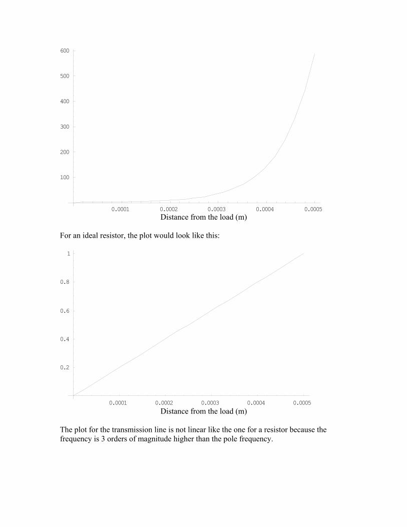
)sinh()()( lVeeVlV ll γγγ +−+ =−= So for R = 106Ω/500µm = 2*109 Ω, C = 100*10-15F/500 µm = 2*1010 F, we can plot the V/V+ vs. the distance from the load.

0.0001 0.0002 0.0003 0.0004 0.0005

100

200

300

400

500

600

Distance from the load (m)

For an ideal resistor, the plot would look like this:

0.0001 0.0002 0.0003 0.0004 0.0005

0.2

0.4

0.6

0.8

1

Distance from the load (m)

The plot for the transmission line is not linear like the one for a resistor because the frequency is 3 orders of magnitude higher than the pole frequency.