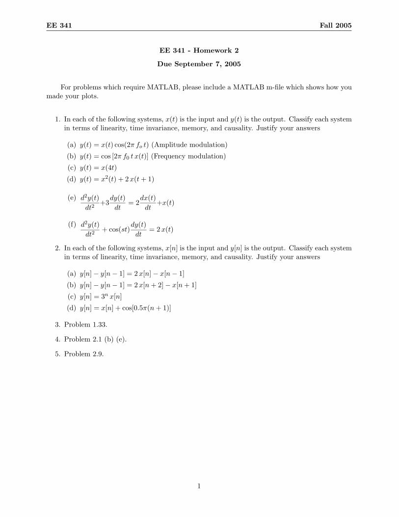
EE 341 Fall 2005

EE 341 - Homework 2

Due September 7, 2005

For problems which require MATLAB, please include a MATLAB m-file which shows how youmade your plots.

1. In each of the following systems, x(t) is the input and y(t) is the output. Classify each systemin terms of linearity, time invariance, memory, and causality. Justify your answers

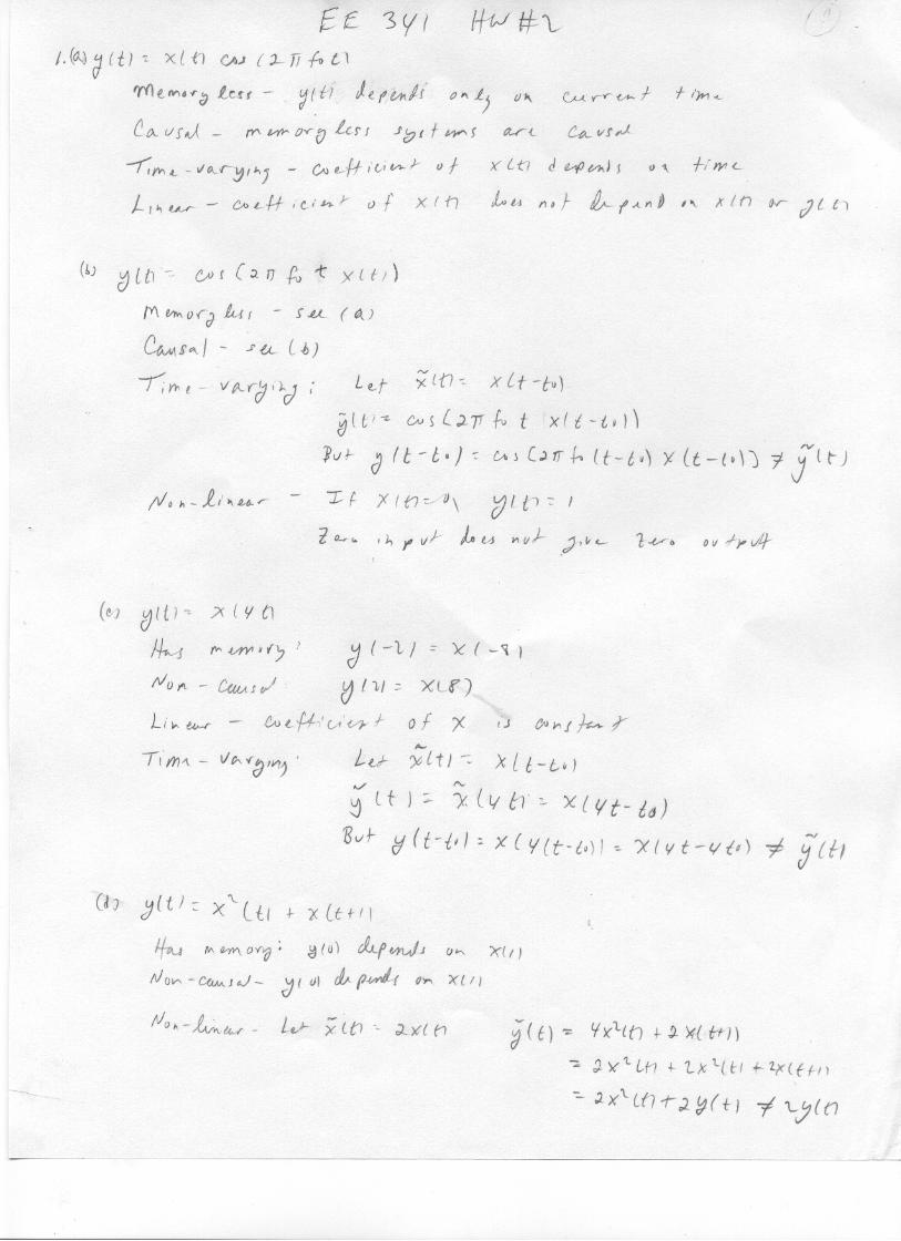
(a) y(t) = x(t) cos(2π fo t) (Amplitude modulation)

(b) y(t) = cos [2π f0 t x(t)] (Frequency modulation)

(c) y(t) = x(4t)

(d) y(t) = x2(t) + 2 x(t + 1)

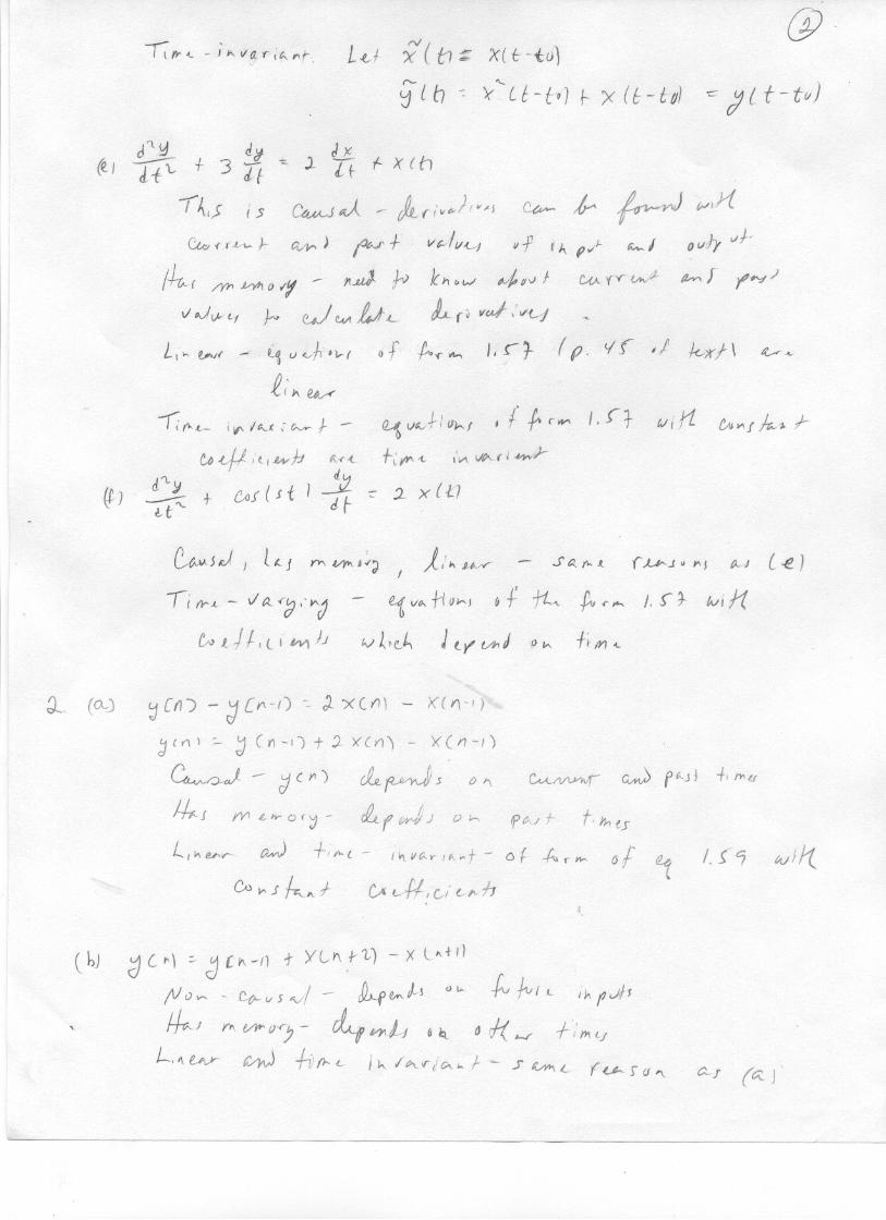
(e) d2y(t)dt2

+3dy(t)dt

= 2dx(t)

dt+x(t)

(f) d2y(t)dt2

+ cos(st)dy(t)dt

= 2x(t)

2. In each of the following systems, x[n] is the input and y[n] is the output. Classify each systemin terms of linearity, time invariance, memory, and causality. Justify your answers

(a) y[n]− y[n− 1] = 2 x[n]− x[n− 1]

(b) y[n]− y[n− 1] = 2 x[n + 2]− x[n + 1]

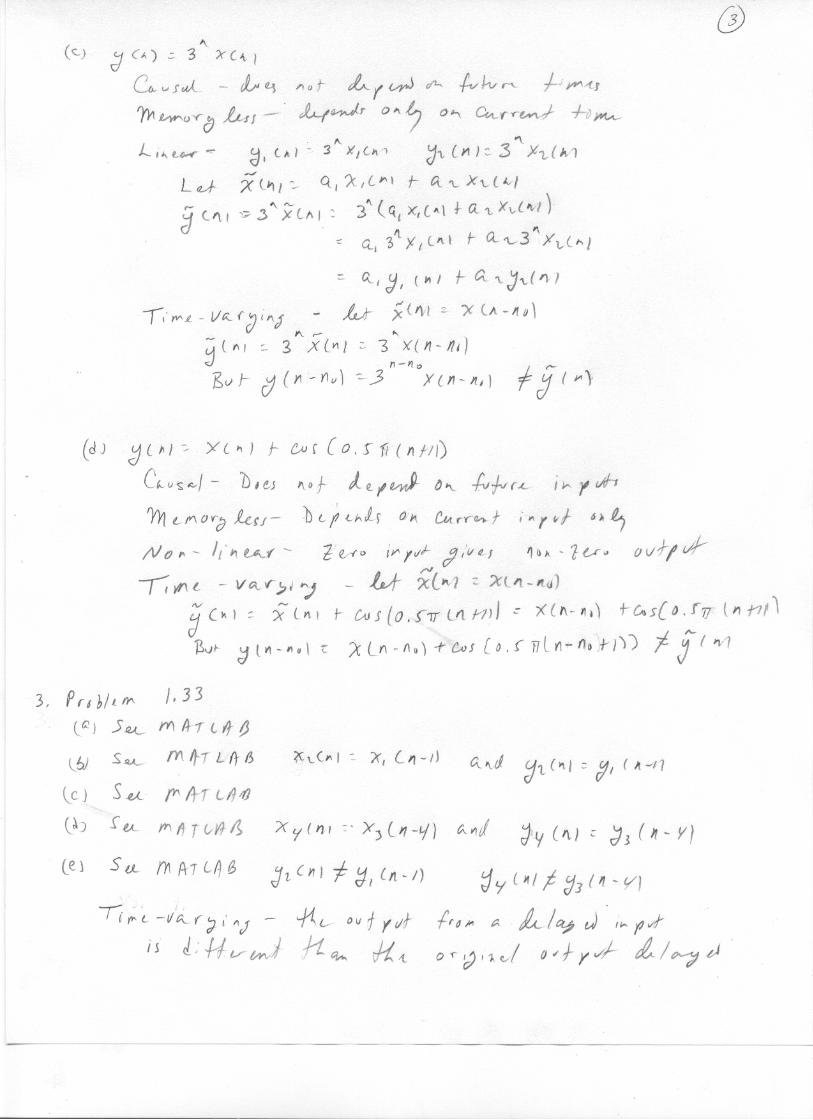
(c) y[n] = 3n x[n]

(d) y[n] = x[n] + cos[0.5π(n + 1)]

3. Problem 1.33.

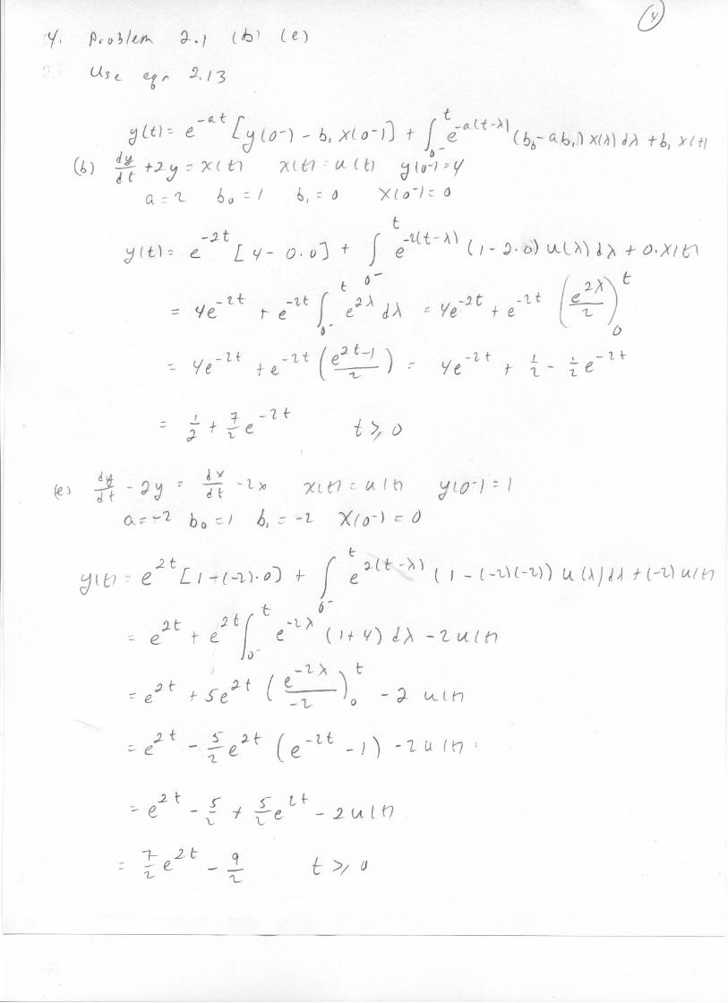
4. Problem 2.1 (b) (e).

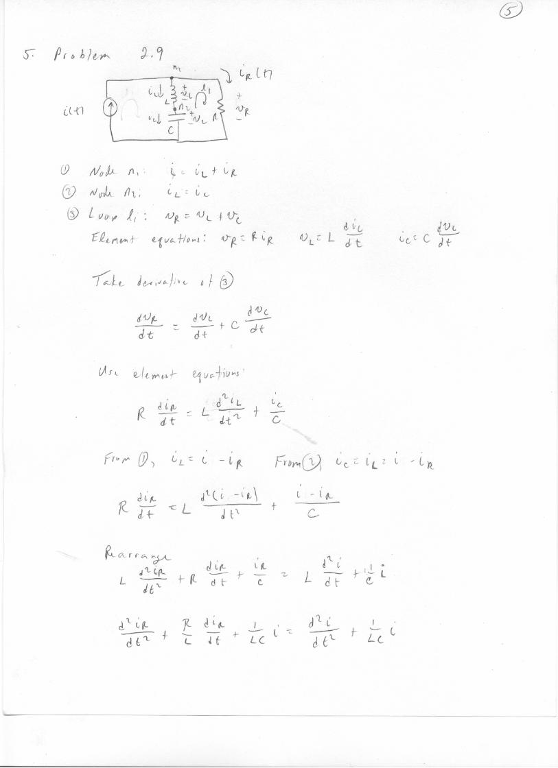
5. Problem 2.9.

1

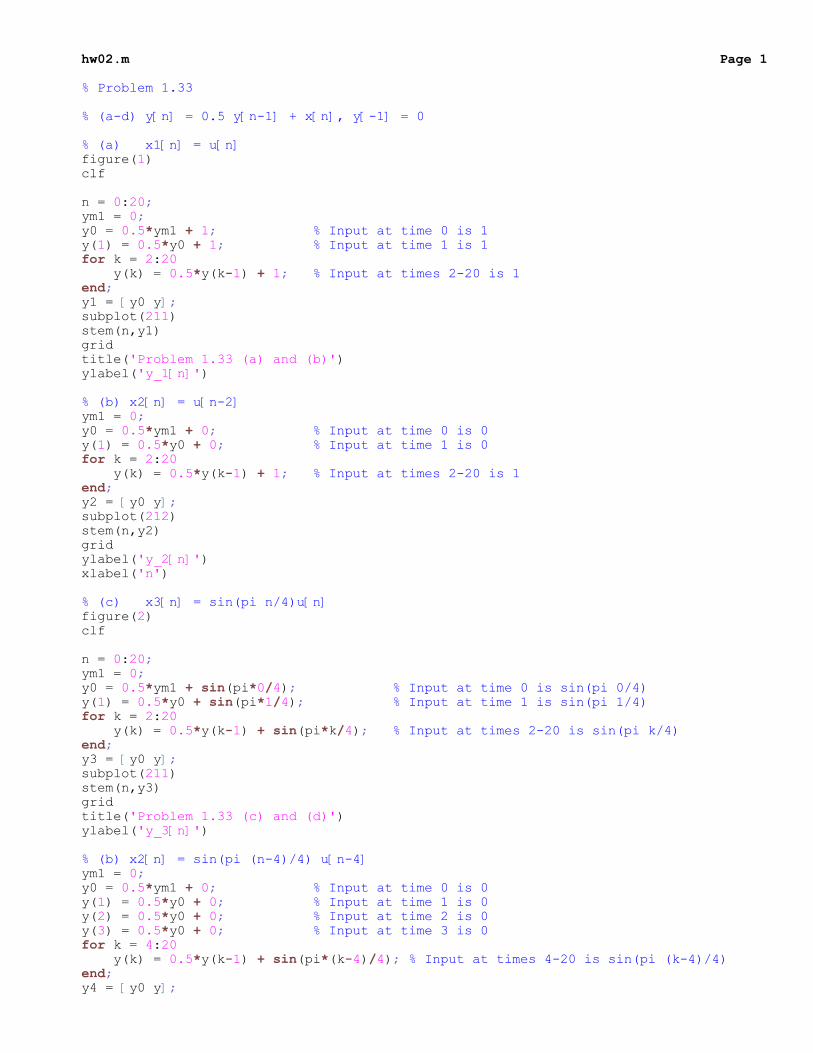
hw02.m Page 1% Problem 1.33

% (a-d) y[n] = 0.5 y[n-1] + x[n], y[-1] = 0

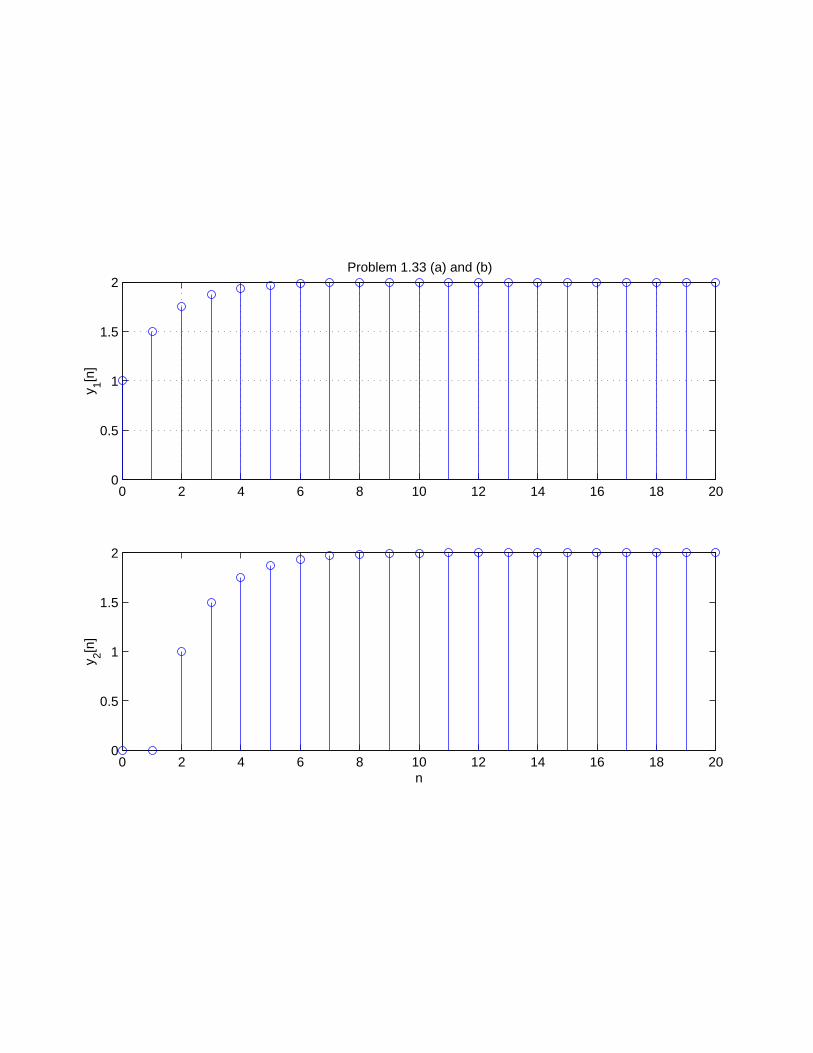
% (a) x1[n] = u[n]figure(1)clf

n = 0:20;ym1 = 0;y0 = 0.5*ym1 + 1; % Input at time 0 is 1y(1) = 0.5*y0 + 1; % Input at time 1 is 1for k = 2:20 y(k) = 0.5*y(k-1) + 1; % Input at times 2-20 is 1end;y1 = [y0 y];subplot(211)stem(n,y1)gridtitle('Problem 1.33 (a) and (b)')ylabel('y_1[n]')

% (b) x2[n] = u[n-2]ym1 = 0;y0 = 0.5*ym1 + 0; % Input at time 0 is 0y(1) = 0.5*y0 + 0; % Input at time 1 is 0for k = 2:20 y(k) = 0.5*y(k-1) + 1; % Input at times 2-20 is 1end;y2 = [y0 y];subplot(212)stem(n,y2)gridylabel('y_2[n]')xlabel('n')

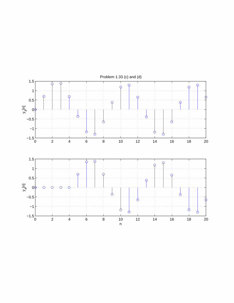
% (c) x3[n] = sin(pi n/4)u[n]figure(2)clf

n = 0:20;ym1 = 0;y0 = 0.5*ym1 + sin(pi*0/4); % Input at time 0 is sin(pi 0/4)y(1) = 0.5*y0 + sin(pi*1/4); % Input at time 1 is sin(pi 1/4)for k = 2:20 y(k) = 0.5*y(k-1) + sin(pi*k/4); % Input at times 2-20 is sin(pi k/4)end;y3 = [y0 y];subplot(211)stem(n,y3)gridtitle('Problem 1.33 (c) and (d)')ylabel('y_3[n]')

% (b) x2[n] = sin(pi (n-4)/4) u[n-4]ym1 = 0;y0 = 0.5*ym1 + 0; % Input at time 0 is 0y(1) = 0.5*y0 + 0; % Input at time 1 is 0y(2) = 0.5*y0 + 0; % Input at time 2 is 0y(3) = 0.5*y0 + 0; % Input at time 3 is 0for k = 4:20 y(k) = 0.5*y(k-1) + sin(pi*(k-4)/4); % Input at times 4-20 is sin(pi (k-4)/4)end;y4 = [y0 y];

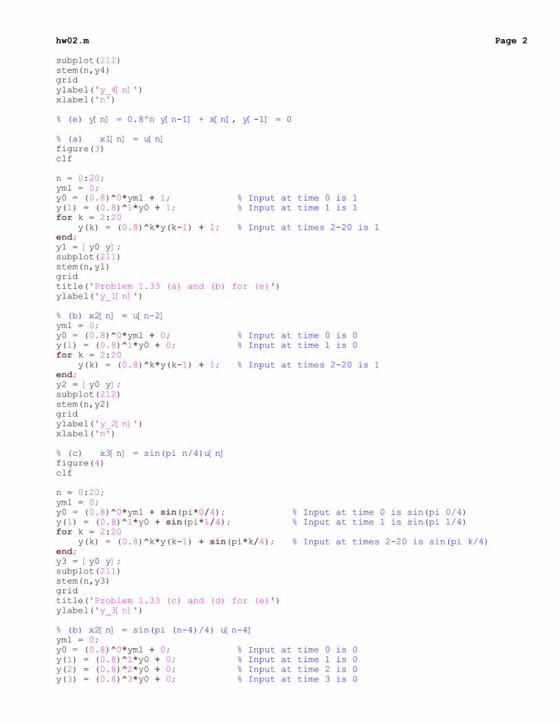
hw02.m Page 2subplot(212)stem(n,y4)gridylabel('y_4[n]')xlabel('n')

% (e) y[n] = 0.8^n y[n-1] + x[n], y[-1] = 0

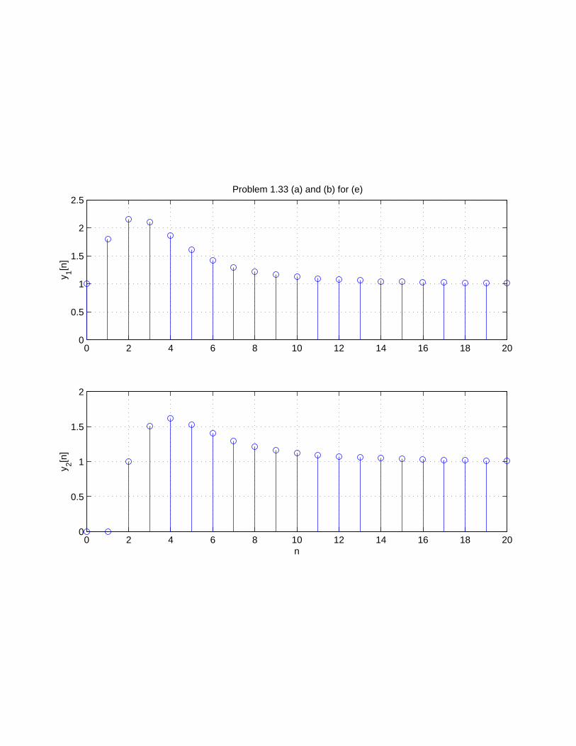
% (a) x1[n] = u[n]figure(3)clf

n = 0:20;ym1 = 0;y0 = (0.8)^0*ym1 + 1; % Input at time 0 is 1y(1) = (0.8)^1*y0 + 1; % Input at time 1 is 1for k = 2:20 y(k) = (0.8)^k*y(k-1) + 1; % Input at times 2-20 is 1end;y1 = [y0 y];subplot(211)stem(n,y1)gridtitle('Problem 1.33 (a) and (b) for (e)')ylabel('y_1[n]')

% (b) x2[n] = u[n-2]ym1 = 0;y0 = (0.8)^0*ym1 + 0; % Input at time 0 is 0y(1) = (0.8)^1*y0 + 0; % Input at time 1 is 0for k = 2:20 y(k) = (0.8)^k*y(k-1) + 1; % Input at times 2-20 is 1end;y2 = [y0 y];subplot(212)stem(n,y2)gridylabel('y_2[n]')xlabel('n')

% (c) x3[n] = sin(pi n/4)u[n]figure(4)clf

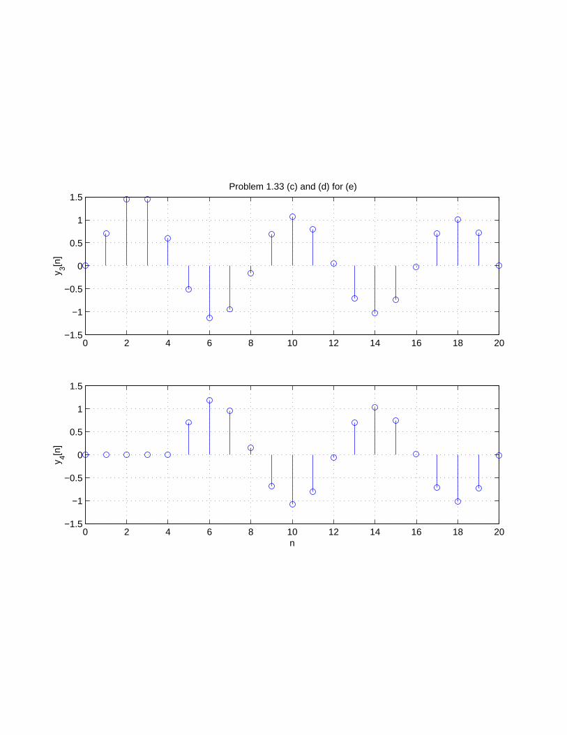
n = 0:20;ym1 = 0;y0 = (0.8)^0*ym1 + sin(pi*0/4); % Input at time 0 is sin(pi 0/4)y(1) = (0.8)^1*y0 + sin(pi*1/4); % Input at time 1 is sin(pi 1/4)for k = 2:20 y(k) = (0.8)^k*y(k-1) + sin(pi*k/4); % Input at times 2-20 is sin(pi k/4)end;y3 = [y0 y];subplot(211)stem(n,y3)gridtitle('Problem 1.33 (c) and (d) for (e)')ylabel('y_3[n]')

% (b) x2[n] = sin(pi (n-4)/4) u[n-4]ym1 = 0;y0 = (0.8)^0*ym1 + 0; % Input at time 0 is 0y(1) = (0.8)^1*y0 + 0; % Input at time 1 is 0y(2) = (0.8)^2*y0 + 0; % Input at time 2 is 0y(3) = (0.8)^3*y0 + 0; % Input at time 3 is 0

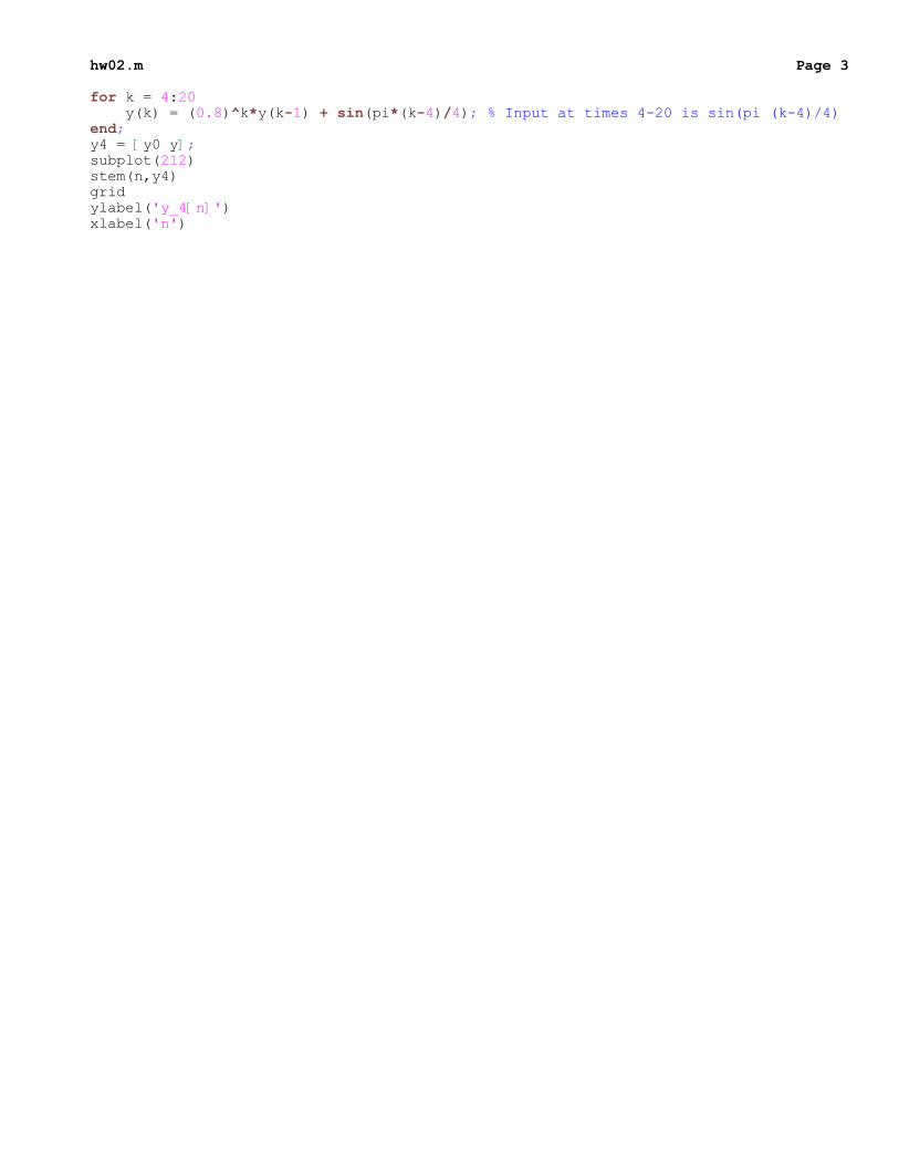
hw02.m Page 3for k = 4:20 y(k) = (0.8)^k*y(k-1) + sin(pi*(k-4)/4); % Input at times 4-20 is sin(pi (k-4)/4)end;y4 = [y0 y];subplot(212)stem(n,y4)gridylabel('y_4[n]')xlabel('n')

0 2 4 6 8 10 12 14 16 18 200

0.5

1

1.5

2Problem 1.33 (a) and (b)

y 1[n]

0 2 4 6 8 10 12 14 16 18 200

0.5

1

1.5

2

y 2[n]

n

0 2 4 6 8 10 12 14 16 18 20−1.5

−1

−0.5

0

0.5

1

1.5Problem 1.33 (c) and (d)

y 3[n]

0 2 4 6 8 10 12 14 16 18 20−1.5

−1

−0.5

0

0.5

1

1.5

y 4[n]

n

0 2 4 6 8 10 12 14 16 18 200

0.5

1

1.5

2

2.5Problem 1.33 (a) and (b) for (e)

y 1[n]

0 2 4 6 8 10 12 14 16 18 200

0.5

1

1.5

2

y 2[n]

n

0 2 4 6 8 10 12 14 16 18 20−1.5

−1

−0.5

0

0.5

1

1.5Problem 1.33 (c) and (d) for (e)

y 3[n]

0 2 4 6 8 10 12 14 16 18 20−1.5

−1

−0.5

0

0.5

1

1.5

y 4[n]

n