
EE 178 Lecture Notes 0 Course Introduction · EE 178 Lecture Notes 0 Course Introduction ... A...
181
EE 178 Lecture Notes 0 Course Introduction • About EE178 • About Probability • Course Goals • Course Topics • Lecture Notes EE 178: Course Introduction Page 0 – 1 EE 178 • EE 178 provides an introduction to probabilistic system analysis: ◦ Basic probability theory ◦ Some statistics ◦ Examples from EE systems • Fulfills the EE undergraduate probability and statistics requirement (alternatives include Stat 116 and Math 151) • Very important background for EEs ◦ Signal processing ◦ Communication ◦ Communication networks ◦ Reliability of systems ◦ Noise in circuits EE 178: Course Introduction Page 0 – 2
Transcript of EE 178 Lecture Notes 0 Course Introduction · EE 178 Lecture Notes 0 Course Introduction ... A...
EE 178 Lecture Notes 0
Course Introduction
• About EE178
• About Probability
• Course Goals
• Course Topics
• Lecture Notes
EE 178: Course Introduction Page 0 – 1
EE 178
• EE 178 provides an introduction to probabilistic system analysis:
Basic probability theory
Some statistics
Examples from EE systems
• Fulfills the EE undergraduate probability and statistics requirement (alternativesinclude Stat 116 and Math 151)
• Very important background for EEs
Signal processing
Communication
Communication networks
Reliability of systems
Noise in circuits
EE 178: Course Introduction Page 0 – 2
• Also important in many other fields, including
Computer science (Artificial intelligence)
Economics
Finance (stock market)
Physics (statistical physics, quantum physics)
Medicine (drug trials)
• Knowledge of probability is almost as necessary as calculus and linear algebra
EE 178: Course Introduction Page 0 – 3
Probability Theory
• Probability provides mathematical models for random phenomena andexperiments, such as: gambling, stock market, packet transmission in networks,electron emission, noise, statistical mechanics, etc.
• Its origin lies in observations associated with games of chance:
If an “unbiased” coin is tossed n times and heads come up nH times, therelative frequency of heads, nH/n, is likely to be very close to 1/2
If a card is drawn from a perfectly shuffled deck and then replaced, the deckis reshuffled, and the process is repeated n times, the relative frequency ofspades is around 1/4
• The purpose of probability theory is to describe and predict such relativefrequencies (averages) in terms of probabilities of events
• But how is probability defined?
EE 178: Course Introduction Page 0 – 4
• Classical definition of probability: This was the prevailing definition for manycenturies.Define the probability of an event A as:
P(A) =NA
N,
where N is the number of possible outcomes of the random experiment and NA
is the number of outcomes favorable to the event AFor example for a 6-sided die there are 6 outcomes and 3 of them are even, thusP(even) = 3/6Problems with this classical definition:
Here the assumption is that all outcomes are equally likely (probable). Thus,the concept of probability is used to define probability itself! Cannot be usedas basis for a mathematical theory
In many random experiments, the outcomes are not equally likely
The definition doesn’t work when the number of possible outcomes is infinite
EE 178: Course Introduction Page 0 – 5
• Relative frequency definition of probability: Here the probability of an event A isdefined as:
P(A) = limn→∞
nA
n,
where nA is the number of times A occurs in n performances of the experiment
Problems with the frequency definition:
How do we assert that such limit exists?
We often cannot perform the experiment multiple times (or even once, e.g.,defining the probability of a nuclear plant failure)
EE 178: Course Introduction Page 0 – 6
Axiomatic Definition of Probability
• The axiomatic definition of probability was introduced by Kolmogorov in 1933. Itprovides rules for assigning probabilities to events in a mathematically consistentway and for deducing probabilities of events from probabilities of other events
• Elements of axiomatic definition:
Set of all possible outcomes of the random experiment Ω (Sample space)
Set of events, which are subsets of Ω
A probability law (measure or function) that assigns probabilities to eventssuch that:1. P(A) ≥ 02. P(Ω) = 1, and3. If A and B are disjoint events, i.e., A ∩B = ∅, then
P(A ∪B) = P(A) + P(B)
• These rules are consistent with relative frequency interpretation
EE 178: Course Introduction Page 0 – 7
• Unlike the relative frequency definition, where the limit is assumed to exist, theaxiomatic approach itself is used to prove when and under what conditions suchlimit exists (Laws of Large Numbers) and how fast it is approached (CentralLimit Theorem)
• The theory provides mathematically precise ways for dealing with experimentswith infinite number of possible outcomes, defining random variables, etc.
• The theory does not deal with what the values of the probabilities are or howthey are obtained. Any assignment of probabilities that satisfies the axioms islegitimate
• How do we find the actual probabilities? They are obtained from:
Physics, e.g., Boltzmann, Bose-Einstein, Fermi-Dirac statistics
Engineering models, e.g., queuing models for communication networks,models for noisy communication channels
Social science theories, e.g., intelligence, behavior
Empirically. Collect data and fit a model (may have no physical, engineering,or social meaning ...)
EE 178: Course Introduction Page 0 – 8
Statistics and Statistical Signal Processing
• Statistics applies probability theory to real world problems. It deals with:
Methods for data collection and construction of experiments described byprobabilistic models, and
Methods for making inferences from data, e.g., estimating probabilities,deciding if a drug is effective from drug trials
• Statistical signal processing:
Develops probabilistic models for EE signals, e.g., speech, audio, images,video, and systems, e.g., communication, storage, compression, errorcorrection, pattern recognition
Uses tools from probability and statistics to design signal processingalgorithms to extract, predict, estimate, detect, compress, . . . such signals
The field has provided the foundation for the Information Age. Its impact onour lives has been huge: cell phones, DSL, digital cameras, DVD, MP3players, digital TV, medical imaging, etc.
EE 178: Course Introduction Page 0 – 9
Course Goals
• Provide an introduction to probability theory (precise but not overlymathematical)
• Provide, through examples, some applications of probability to EE systems
• Provide some exposure to statistics and statistical signal processing
• Provide background for more advanced courses in statistical signal processingand communication (e.g., EE 278, 279)
• Have a lot of fun solving cool probability problems
WARNING: To really understand probability you have to work homeworkproblems yourself. Just reading solutions or having others give you solutionswill not do
EE 178: Course Introduction Page 0 – 10
Course Outline
1. Sample Space and probability (B&T: Chapter 1)
• Set theory• Sample space: discrete, continuous• Events• Probability law• Conditional probability; chain rule• Law of total probability• Bayes rule• Independence• Counting
EE 178: Course Introduction Page 0 – 11
2. Random Variables (B&T: 2.1–2.4, 3.1–3.3, 3.6 pp. 179–186)
• Basic concepts• Probability mass function (pmf)• Famous discrete random variables• Probability density function (pdf)• Famous continuous random variables• Mean and variance• Cumulative distribution function (cdf)• Functions of random variables
3. Multiple Random variables (B&T: 2.5–2.7, 3.4–3.5, 3.6 pp. 186–190, 4.2)
• Joint, marginal, and conditional pmf: Bayes rule for pmfs, independence• Joint, marginal, and conditional pdf: Bayes rule for pdfs, independence• Functions of multiple random variables
EE 178: Course Introduction Page 0 – 12
4. Expectation: (B&T: 2.4, 3.1, pp. 144–148, 4.3, 4.5, 4.6)
• Definition and properties• Correlation and covariance• Sum of random variables• Conditional expectation• Iterated expectation• Mean square error estimation
5. Transforms (B&T: 4.1)
6. Limit Theorems (B&T: 7.1, 7.2, 4.1, 7.4)
• Sample mean• Markov and Chebychev inequalities• Weak law of large numbers• The Central Limit Theorem• Confidence Intervals
EE 178: Course Introduction Page 0 – 13
7. Random Processes: (B&T: 5.1, 6.1–6.4)
• Basic concepts• Bernoulli process• Markov chains
EE 178: Course Introduction Page 0 – 14

Lecture Notes
• Based on B&T text, Prof. Gray EE 178 notes, and other sources
• Help organize the material and reduce note taking in lectures
• You will need to take some notes, e.g. clarifications, missing steps inderivations, solutions to additional examples
• Slide title indicates a topic that often continues over several consecutive slides
• Lecture notes + your notes + review sessions should be sufficient (B&T is onlyrecommended)
EE 178: Course Introduction Page 0 – 15
EE 178 Lecture Notes 1
Basic Probability
• Set Theory
• Elements of Probability
• Conditional probability
• Sequential Calculation of Probability
• Total Probability and Bayes Rule
• Independence
• Counting
EE 178: Basic Probability Page 1 – 1
Set Theory Basics
• A set is a collection of objects, which are its elements
ω ∈ A means that ω is an element of the set A
A set with no elements is called the empty set, denoted by ∅
• Types of sets:
Finite: A = ω1, ω2, . . . , ωn
Countably infinite: A = ω1, ω2, . . ., e.g., the set of integers
Uncountable: A set that takes a continuous set of values, e.g., the [0, 1]interval, the real line, etc.
• A set can be described by all ω having a certain property, e.g., A = [0, 1] can bewritten as A = ω : 0 ≤ ω ≤ 1
• A set B ⊂ A means that every element of B is an element of A
• A universal set Ω contains all objects of particular interest in a particularcontext, e.g., sample space for random experiment
EE 178: Basic Probability Page 1 – 2
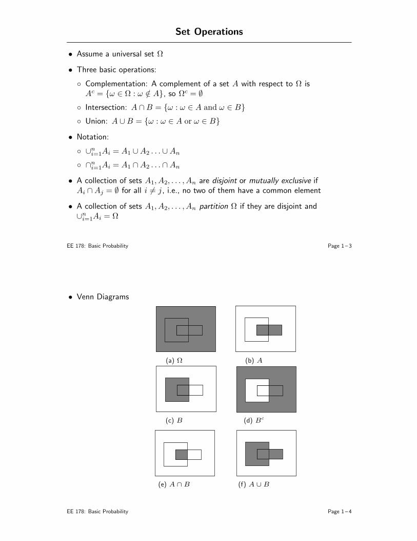
Set Operations
• Assume a universal set Ω
• Three basic operations:
Complementation: A complement of a set A with respect to Ω isAc = ω ∈ Ω : ω /∈ A, so Ωc = ∅
Intersection: A ∩B = ω : ω ∈ A and ω ∈ B
Union: A ∪B = ω : ω ∈ A or ω ∈ B
• Notation:
∪ni=1Ai = A1 ∪A2 . . . ∪An
∩ni=1Ai = A1 ∩A2 . . . ∩An
• A collection of sets A1, A2, . . . , An are disjoint or mutually exclusive ifAi ∩Aj = ∅ for all i 6= j , i.e., no two of them have a common element
• A collection of sets A1, A2, . . . , An partition Ω if they are disjoint and∪ni=1Ai = Ω
EE 178: Basic Probability Page 1 – 3
• Venn Diagrams
(e) A ∩ B (f) A ∪ B
(b) A
(d) Bc
(a) Ω
(c) B
EE 178: Basic Probability Page 1 – 4
Algebra of Sets
• Basic relations:
1. S ∩ Ω = S
2. (Ac)c = A
3. A ∩Ac = ∅
4. Commutative law: A ∪B = B ∪A
5. Associative law: A ∪ (B ∪ C) = (A ∪B) ∪ C
6. Distributive law: A ∩ (B ∪ C) = (A ∩B) ∪ (A ∩ C)
7. DeMorgan’s law: (A ∩B)c = Ac ∪Bc
DeMorgan’s law can be generalized to n events:
(∩ni=1Ai)
c= ∪n
i=1Aci
• These can all be proven using the definition of set operations or visualized usingVenn Diagrams
EE 178: Basic Probability Page 1 – 5
Elements of Probability
• Probability theory provides the mathematical rules for assigning probabilities tooutcomes of random experiments, e.g., coin flips, packet arrivals, noise voltage
• Basic elements of probability:
Sample space: The set of all possible “elementary” or “finest grain”outcomes of the random experiment (also called sample points)– The sample points are all disjoint– The sample points are collectively exhaustive, i.e., together they make upthe entire sample space
Events: Subsets of the sample space
Probability law : An assignment of probabilities to events in a mathematicallyconsistent way
EE 178: Basic Probability Page 1 – 6

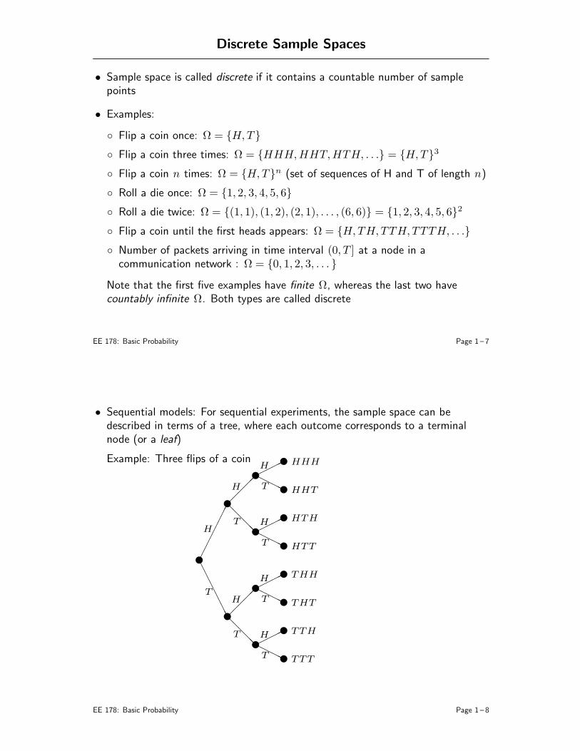
Discrete Sample Spaces
• Sample space is called discrete if it contains a countable number of samplepoints
• Examples:
Flip a coin once: Ω = H, T
Flip a coin three times: Ω = HHH,HHT,HTH, . . . = H,T3
Flip a coin n times: Ω = H,Tn (set of sequences of H and T of length n)
Roll a die once: Ω = 1, 2, 3, 4, 5, 6
Roll a die twice: Ω = (1, 1), (1, 2), (2, 1), . . . , (6, 6) = 1, 2, 3, 4, 5, 62
Flip a coin until the first heads appears: Ω = H,TH, TTH, TTTH, . . .
Number of packets arriving in time interval (0, T ] at a node in acommunication network : Ω = 0, 1, 2, 3, . . .
Note that the first five examples have finite Ω, whereas the last two havecountably infinite Ω. Both types are called discrete
EE 178: Basic Probability Page 1 – 7
• Sequential models: For sequential experiments, the sample space can bedescribed in terms of a tree, where each outcome corresponds to a terminalnode (or a leaf)
Example: Three flips of a coin
|
H
|
H
|
@@@@@@
T|
AAAAAAAAAAA
T
|
H
|
@@@@@@
T|
HHHHHHHT
HHHHHHHT
HHHHHHHT
HHHHHHHT
|HHH
|HHT
|HTH
|HTT
|THH
|THT
|TTH
|TTT
EE 178: Basic Probability Page 1 – 8
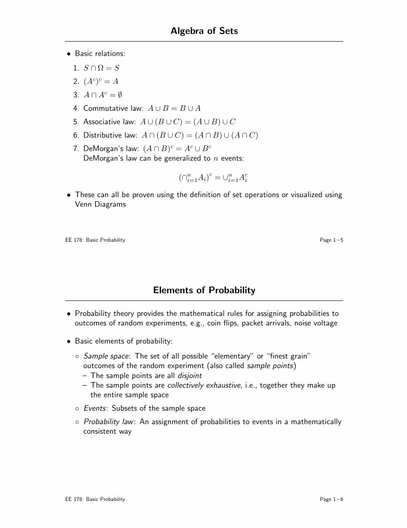
• Example: Roll a fair four-sided die twice.
Sample space can be represented by a tree as above, or graphically
f
f
f
f
f
f
f
f
f
f
f
f
f
f
f
f
2nd roll
1st roll
1
2
3
4
1 2 3 4
EE 178: Basic Probability Page 1 – 9
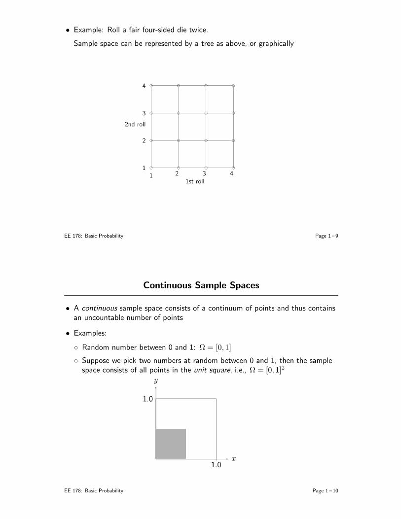
Continuous Sample Spaces
• A continuous sample space consists of a continuum of points and thus containsan uncountable number of points
• Examples:
Random number between 0 and 1: Ω = [0, 1]
Suppose we pick two numbers at random between 0 and 1, then the samplespace consists of all points in the unit square, i.e., Ω = [0, 1]2
6
-
1.0
1.0x
y
EE 178: Basic Probability Page 1 – 10
Packet arrival time: t ∈ (0,∞), thus Ω = (0,∞)
Arrival times for n packets: ti ∈ (0,∞), for i = 1, 2, . . . , n, thus Ω = (0,∞)n
• A sample space is said to be mixed if it is neither discrete nor continuous, e.g.,Ω = [0, 1] ∪ 3
EE 178: Basic Probability Page 1 – 11
Events
• Events are subsets of the sample space. An event occurs if the outcome of theexperiment belongs to the event
• Examples:
Any outcome (sample point) is an event (also called an elementary event),e.g., HTH in three coin flips experiment or 0.35 in the picking of arandom number between 0 and 1 experiment
Flip coin 3 times and get exactly one H. This is a more complicated event,consisting of three sample points TTH, THT, HTT
Flip coin 3 times and get an odd number of H’s. The event isTTH, THT, HTT, HHH
Pick a random number between 0 and 1 and get a number between 0.0 and0.5. The event is [0, 0.5]
• An event might have no points in it, i.e., be the empty set ∅
EE 178: Basic Probability Page 1 – 12
Axioms of Probability
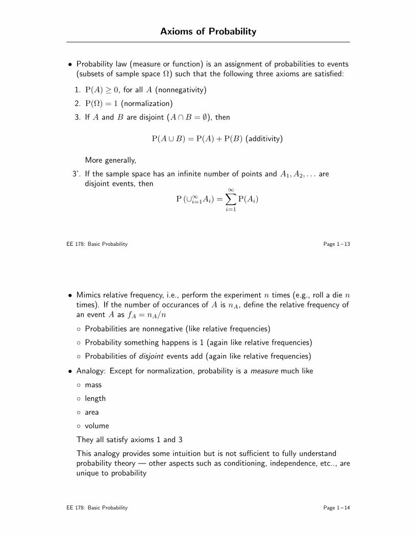
• Probability law (measure or function) is an assignment of probabilities to events(subsets of sample space Ω) such that the following three axioms are satisfied:
1. P(A) ≥ 0, for all A (nonnegativity)
2. P(Ω) = 1 (normalization)
3. If A and B are disjoint (A ∩B = ∅), then
P(A ∪B) = P(A) + P(B) (additivity)
More generally,
3’. If the sample space has an infinite number of points and A1, A2, . . . aredisjoint events, then
P (∪∞
i=1Ai) =∞∑
i=1
P(Ai)
EE 178: Basic Probability Page 1 – 13
• Mimics relative frequency, i.e., perform the experiment n times (e.g., roll a die ntimes). If the number of occurances of A is nA, define the relative frequency ofan event A as fA = nA/n
Probabilities are nonnegative (like relative frequencies)
Probability something happens is 1 (again like relative frequencies)
Probabilities of disjoint events add (again like relative frequencies)
• Analogy: Except for normalization, probability is a measure much like
mass
length
area
volume
They all satisfy axioms 1 and 3
This analogy provides some intuition but is not sufficient to fully understandprobability theory — other aspects such as conditioning, independence, etc.., areunique to probability
EE 178: Basic Probability Page 1 – 14
Probability for Discrete Sample Spaces
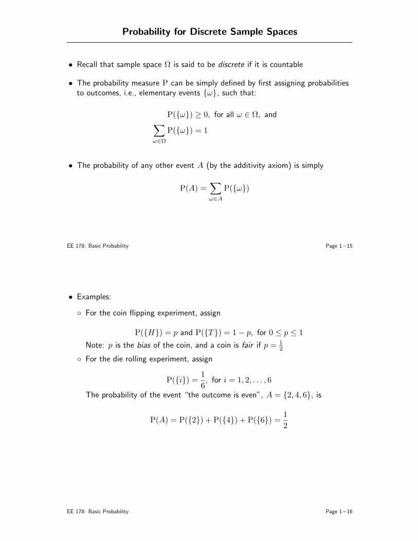
• Recall that sample space Ω is said to be discrete if it is countable
• The probability measure P can be simply defined by first assigning probabilitiesto outcomes, i.e., elementary events ω, such that:
P(ω) ≥ 0, for all ω ∈ Ω, and∑
ω∈Ω
P(ω) = 1
• The probability of any other event A (by the additivity axiom) is simply
P(A) =∑
ω∈A
P(ω)
EE 178: Basic Probability Page 1 – 15
• Examples:
For the coin flipping experiment, assign
P(H) = p and P(T) = 1− p, for 0 ≤ p ≤ 1
Note: p is the bias of the coin, and a coin is fair if p = 12
For the die rolling experiment, assign
P(i) =1
6, for i = 1, 2, . . . , 6
The probability of the event “the outcome is even”, A = 2, 4, 6, is
P(A) = P(2) + P(4) + P(6) =1
2
EE 178: Basic Probability Page 1 – 16

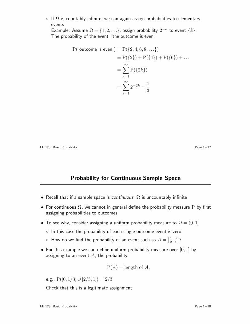
If Ω is countably infinite, we can again assign probabilities to elementaryeventsExample: Assume Ω = 1, 2, . . ., assign probability 2−k to event kThe probability of the event “the outcome is even”
P( outcome is even ) = P(2, 4, 6, 8, . . .)
= P(2) + P(4) + P(6) + . . .
=∞∑
k=1
P(2k)
=∞∑
k=1
2−2k =1
3
EE 178: Basic Probability Page 1 – 17
Probability for Continuous Sample Space
• Recall that if a sample space is continuous, Ω is uncountably infinite
• For continuous Ω, we cannot in general define the probability measure P by firstassigning probabilities to outcomes
• To see why, consider assigning a uniform probability measure to Ω = (0, 1]
In this case the probability of each single outcome event is zero
How do we find the probability of an event such as A =[
12,
34
]
?
• For this example we can define uniform probability measure over [0, 1] byassigning to an event A, the probability
P(A) = length of A,
e.g., P([0, 1/3] ∪ [2/3, 1]) = 2/3
Check that this is a legitimate assignment
EE 178: Basic Probability Page 1 – 18

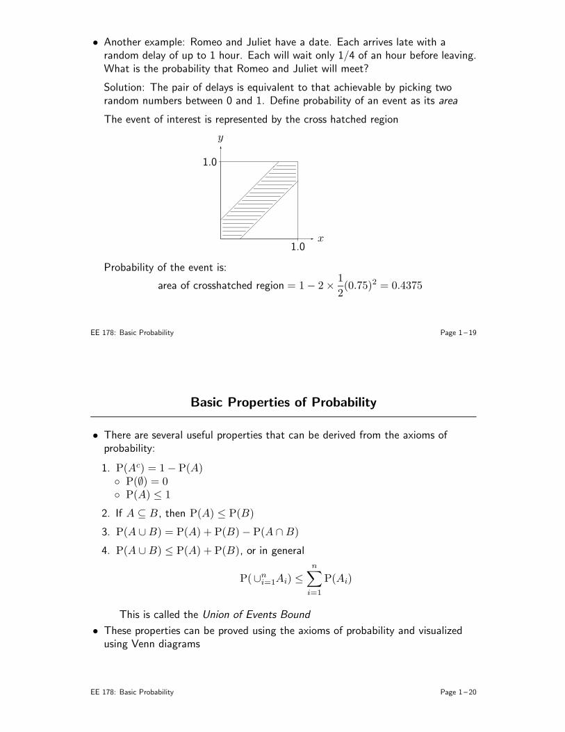
• Another example: Romeo and Juliet have a date. Each arrives late with arandom delay of up to 1 hour. Each will wait only 1/4 of an hour before leaving.What is the probability that Romeo and Juliet will meet?
Solution: The pair of delays is equivalent to that achievable by picking tworandom numbers between 0 and 1. Define probability of an event as its area
The event of interest is represented by the cross hatched region
6
-
1.0
1.0x
y
Probability of the event is:
area of crosshatched region = 1− 2×1
2(0.75)2 = 0.4375
EE 178: Basic Probability Page 1 – 19
Basic Properties of Probability
• There are several useful properties that can be derived from the axioms ofprobability:
1. P(Ac) = 1− P(A) P(∅) = 0 P(A) ≤ 1
2. If A ⊆ B , then P(A) ≤ P(B)
3. P(A ∪B) = P(A) + P(B)− P(A ∩ B)
4. P(A ∪B) ≤ P(A) + P(B), or in general
P(∪ni=1Ai) ≤
n∑
i=1
P(Ai)
This is called the Union of Events Bound
• These properties can be proved using the axioms of probability and visualizedusing Venn diagrams
EE 178: Basic Probability Page 1 – 20

Conditional Probability
• Conditional probability allows us to compute probabilities of events based onpartial knowledge of the outcome of a random experiment
• Examples:
We are told that the sum of the outcomes from rolling a die twice is 9. Whatis the probability the outcome of the first die was a 6?
A spot shows up on a radar screen. What is the probability that there is anaircraft?
You receive a 0 at the output of a digital communication system. What is theprobability that a 0 was sent?
• As we shall see, conditional probability provides us with two methods forcomputing probabilities of events: the sequential method and thedivide-and-conquer method
• It is also the basis of inference in statistics: make an observation and reasonabout the cause
EE 178: Basic Probability Page 1 – 21
• In general, given an event B has occurred, we wish to find the probability ofanother event A, P(A|B)
• If all elementary outcomes are equally likely, then
P(A|B) =# of outcomes in both A and B
# of outcomes in B
• In general, if B is an event such that P(B) 6= 0, the conditional probability ofany event A given B is defined as
P(A|B) =P(A ∩B)
P(B), or
P(A,B)
P(B)
• The function P(·|B) for fixed B specifies a probability law, i.e., it satisfies theaxioms of probability
EE 178: Basic Probability Page 1 – 22

Example
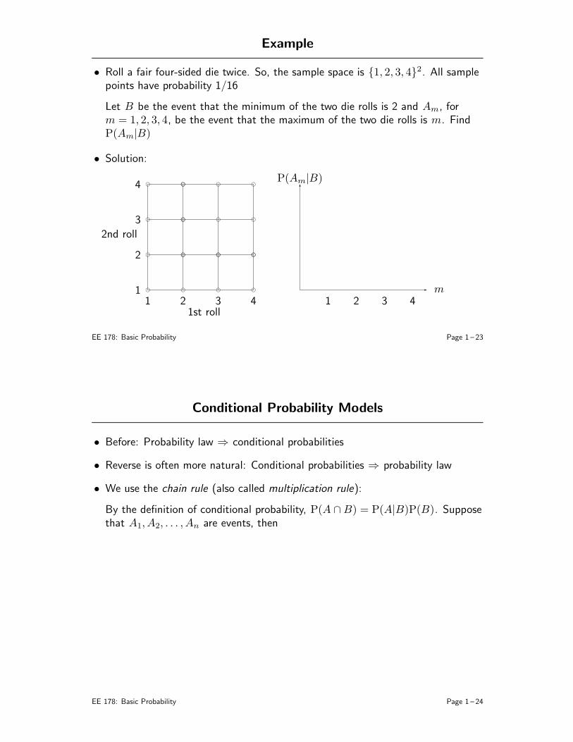
• Roll a fair four-sided die twice. So, the sample space is 1, 2, 3, 42. All samplepoints have probability 1/16
Let B be the event that the minimum of the two die rolls is 2 and Am, form = 1, 2, 3, 4, be the event that the maximum of the two die rolls is m. FindP(Am|B)
• Solution:
f
f
f
f
f
f
f
f
f
f
f
f
f
f
f
f
f
f
f
f f
2nd roll
1st roll
1
2
3
4
1 2 3 4
-
6
m
P(Am|B)
1 2 3 4
EE 178: Basic Probability Page 1 – 23
Conditional Probability Models
• Before: Probability law ⇒ conditional probabilities
• Reverse is often more natural: Conditional probabilities ⇒ probability law
• We use the chain rule (also called multiplication rule):
By the definition of conditional probability, P(A ∩B) = P(A|B)P(B). Supposethat A1, A2, . . . , An are events, then
EE 178: Basic Probability Page 1 – 24

P(A1 ∩A2 ∩A3 · · · ∩An)
= P(A1 ∩A2 ∩A3 · · · ∩An−1)× P(An|A1 ∩A2 ∩ A3 · · · ∩An−1)
= P(A1 ∩A2 ∩A3 · · · ∩An−2)× P(An−1|A1 ∩A2 ∩A3 · · · ∩An−2)
× P(An|A1 ∩A2 ∩A3 · · · ∩An−1)
...
= P(A1)× P(A2|A1)× P(A3|A1 ∩A2) · · ·P(An|A1 ∩A2 ∩A3 · · · ∩An−1)
=n∏
i=1
P(Ai|A1, A2, . . . , Ai−1),
where A0 = ∅
EE 178: Basic Probability Page 1 – 25
Sequential Calculation of Probabilities
• Procedure:
1. Construct a tree description of the sample space for a sequential experiment
2. Assign the conditional probabilities on the corresponding branches of the tree
3. By the chain rule, the probability of an outcome can be obtained bymultiplying the conditional probabilities along the path from the root to theleaf node corresponding to the outcome
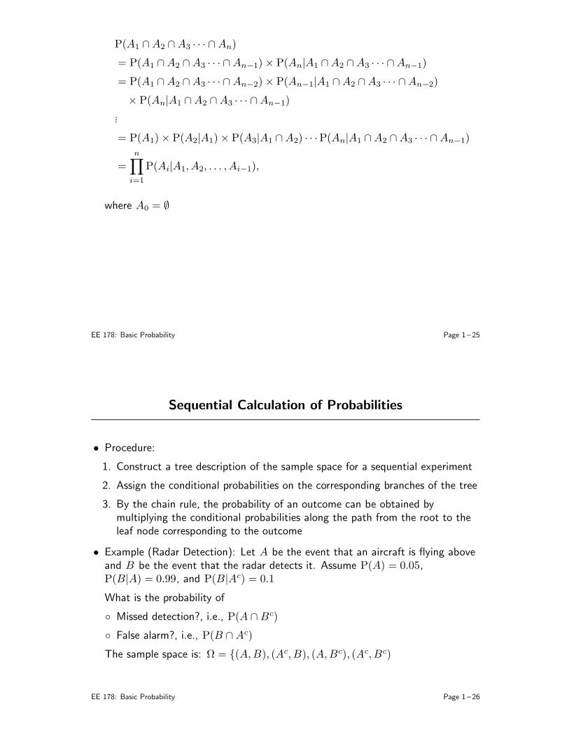
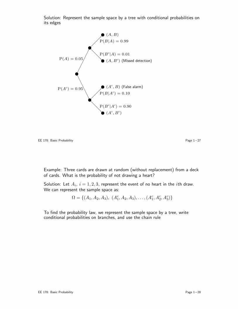
• Example (Radar Detection): Let A be the event that an aircraft is flying aboveand B be the event that the radar detects it. Assume P(A) = 0.05,P(B|A) = 0.99, and P(B|Ac) = 0.1
What is the probability of
Missed detection?, i.e., P(A ∩ Bc)
False alarm?, i.e., P(B ∩Ac)
The sample space is: Ω = (A,B), (Ac, B), (A,Bc), (Ac, Bc)
EE 178: Basic Probability Page 1 – 26

Solution: Represent the sample space by a tree with conditional probabilities onits edges
P(A) = 0.05
P(B|A) = 0.99
@@@@@@
P(Bc|A) = 0.01
(A,B)
AAAAAAAAAAAA
P(Ac) = 0.95
P(B|Ac) = 0.10
(A,Bc) (Missed detection)
@@@@@@
P(Bc|Ac) = 0.90
(Ac, B) (False alarm)
(Ac, Bc)
EE 178: Basic Probability Page 1 – 27
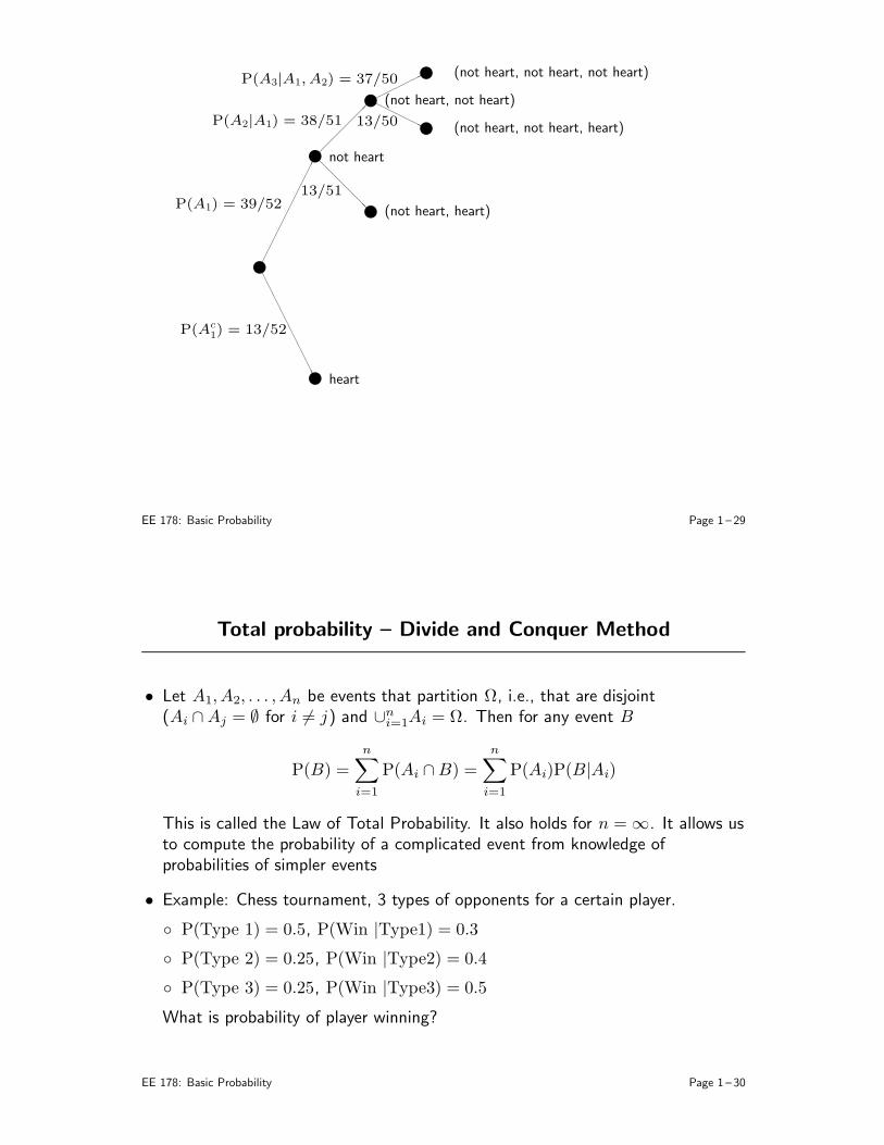
Example: Three cards are drawn at random (without replacement) from a deckof cards. What is the probability of not drawing a heart?
Solution: Let Ai, i = 1, 2, 3, represent the event of no heart in the ith draw.We can represent the sample space as:
Ω = (A1, A2, A3), (Ac1, A2, A3), . . . , (A
c1, A
c2, A
c3)
To find the probability law, we represent the sample space by a tree, writeconditional probabilities on branches, and use the chain rule
EE 178: Basic Probability Page 1 – 28

~
P(A1) = 39/52
not heart~
P(A2|A1) = 38/51
(not heart, not heart)~
@@@@@@@
13/51
(not heart, heart)~
AAAAAAAAAAAAAA
P(Ac1) = 13/52
heart~
P(A3|A1, A2) = 37/50 (not heart, not heart, not heart)
HHHHHHH13/50 (not heart, not heart, heart)
~
~
EE 178: Basic Probability Page 1 – 29
Total probability – Divide and Conquer Method
• Let A1, A2, . . . , An be events that partition Ω, i.e., that are disjoint(Ai ∩Aj = ∅ for i 6= j) and ∪n
i=1Ai = Ω. Then for any event B
P(B) =n∑
i=1
P(Ai ∩B) =n∑
i=1
P(Ai)P(B|Ai)
This is called the Law of Total Probability. It also holds for n = ∞. It allows usto compute the probability of a complicated event from knowledge ofprobabilities of simpler events
• Example: Chess tournament, 3 types of opponents for a certain player.
P(Type 1) = 0.5, P(Win |Type1) = 0.3
P(Type 2) = 0.25, P(Win |Type2) = 0.4
P(Type 3) = 0.25, P(Win |Type3) = 0.5
What is probability of player winning?
EE 178: Basic Probability Page 1 – 30

Solution: Let B be the event of winning and Ai be the event of playing Type i,i = 1, 2, 3:
P(B) =3
∑
i=1
P(Ai)P(B|Ai)
= 0.5× 0.3 + 0.25× 0.4 + 0.25× 0.5
= 0.375
EE 178: Basic Probability Page 1 – 31
Bayes Rule
• Let A1, A2, . . . , An be nonzero probability events (the causes) that partition Ω,and let B be a nonzero probability event (the effect)
• We often know the a priori probabilities P(Ai), i = 1, 2, . . . , n and theconditional probabilities P(B|Ai)s and wish to find the a posteriori probabilities
P(Aj|B) for j = 1, 2, . . . , n
• From the definition of conditional probability, we know that
P(Aj|B) =P(B,Aj)
P(B)=
P(B|Aj)
P(B)P(Aj)
By the law of total probability
P(B) =n∑
i=1
P(Ai)P(B|Ai)
EE 178: Basic Probability Page 1 – 32
Substituting we obtain Bayes rule
P(Aj|B) =P(B|Aj)
∑ni=1P(Ai)P(B|Ai)
P(Aj) for j = 1, 2, . . . , n
• Bayes rule also applies when the number of events n = ∞
• Radar Example: Recall that A is event that the aircraft is flying above and B isthe event that the aircraft is detected by the radar. What is the probability thatan aircraft is actually there given that the radar indicates a detection?
Recall P(A) = 0.05, P(B|A) = 0.99, P(B|Ac) = 0.1. Using Bayes rule:
P(there is an aircraft|radar detects it) = P(A|B)
=P(B|A)P(A)
P(B|A)P(A) + P(B|Ac)P(Ac)
=0.05× 0.99
0.05× 0.99 + 0.95× 0.1
= 0.3426
EE 178: Basic Probability Page 1 – 33
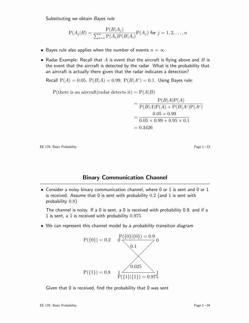
Binary Communication Channel
• Consider a noisy binary communication channel, where 0 or 1 is sent and 0 or 1is received. Assume that 0 is sent with probability 0.2 (and 1 is sent withprobability 0.8)
The channel is noisy. If a 0 is sent, a 0 is received with probability 0.9, and if a1 is sent, a 1 is received with probability 0.975
• We can represent this channel model by a probability transition diagram
00
1 1
P(0|0) = 0.9
P(1|1) = 0.975
P(0) = 0.2
P(1) = 0.8
0.1
0.025
Given that 0 is received, find the probability that 0 was sent
EE 178: Basic Probability Page 1 – 34
• This is a random experiment with sample space Ω = (0, 0), (0, 1), (1, 0), (1, 1),where the first entry is the bit sent and the second is the bit received
• Define the two events
A = 0 is sent = (0, 1), (0, 0), and
B = 0 is received = (0, 0), (1, 0)
• The probability measure is defined via the P(A), P(B|A), and P(Bc|Ac)provided on the probability transition diagram of the channel
• To find P(A|B), the a posteriori probability that a 0 was sent. We use Bayesrule
P(A|B) =P(B|A)P(A)
P(A)P(B|A) + P(Ac)P(B|Ac),
to obtain
P(A|B) =0.9
0.2× 0.2 = 0.9,
which is much higher than the a priori probability of A (= 0.2)
EE 178: Basic Probability Page 1 – 35
Independence
• It often happens that the knowledge that a certain event B has occurred has noeffect on the probability that another event A has occurred, i.e.,
P(A|B) = P(A)
In this case we say that the two events are statistically independent
• Equivalently, two events are said to be statistically independent if
P(A,B) = P(A)P(B)
So, in this case, P(A|B) = P(A) and P(B|A) = P(B)
• Example: Assuming that the binary channel of the previous example is used tosend two bits independently, what is the probability that both bits are in error?
EE 178: Basic Probability Page 1 – 36
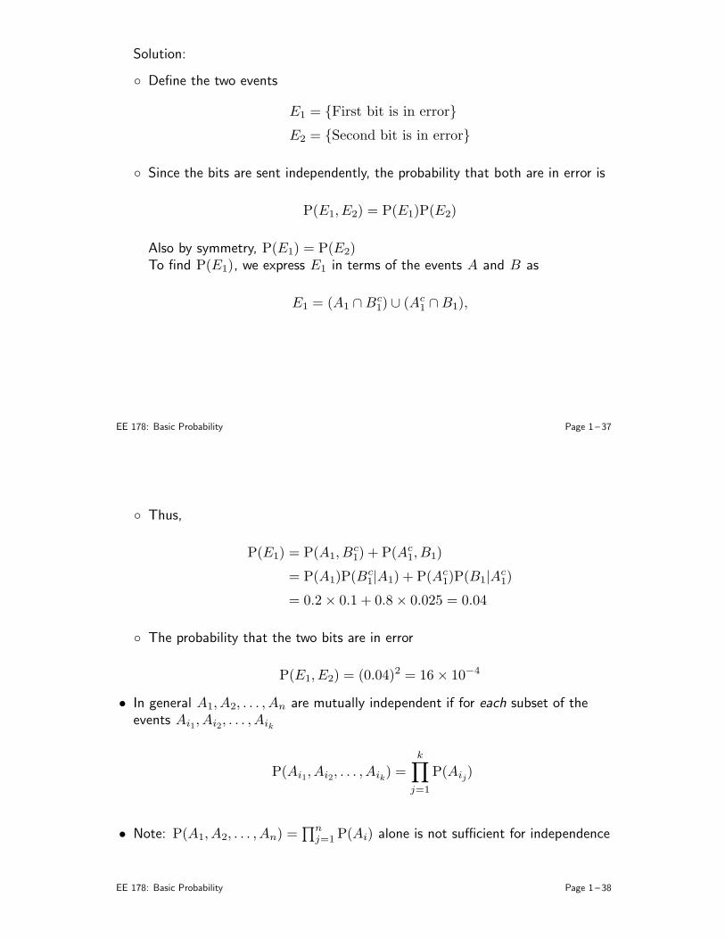
Solution:
Define the two events
E1 = First bit is in error
E2 = Second bit is in error
Since the bits are sent independently, the probability that both are in error is
P(E1, E2) = P(E1)P(E2)
Also by symmetry, P(E1) = P(E2)To find P(E1), we express E1 in terms of the events A and B as
E1 = (A1 ∩Bc1) ∪ (Ac
1 ∩B1),
EE 178: Basic Probability Page 1 – 37
Thus,
P(E1) = P(A1, Bc1) + P(Ac
1, B1)
= P(A1)P(Bc1|A1) + P(Ac
1)P(B1|Ac1)
= 0.2× 0.1 + 0.8× 0.025 = 0.04
The probability that the two bits are in error
P(E1, E2) = (0.04)2 = 16× 10−4
• In general A1, A2, . . . , An are mutually independent if for each subset of theevents Ai1, Ai2, . . . , Aik
P(Ai1, Ai2, . . . , Aik) =k∏
j=1
P(Aij)
• Note: P(A1, A2, . . . , An) =∏n
j=1P(Ai) alone is not sufficient for independence
EE 178: Basic Probability Page 1 – 38

Example: Roll two fair dice independently. Define the events
A = First die = 1, 2, or 3
B = First die = 2, 3, or 6
C = Sum of outcomes = 9
Are A, B , and C independent?
EE 178: Basic Probability Page 1 – 39
Solution:
Since the dice are fair and the experiments are performed independently, theprobability of any pair of outcomes is 1/36, and
P(A) =1
2, P(B) =
1
2, P(C) =
1
9
Since A ∩B ∩ C = (3, 6), P(A,B,C) = 136 = P(A)P(B)P(C)
But are A, B , and C independent? Let’s find
P(A,B) =2
6=
1
36=
1
4= P(A)P(B),
and thus A, B , and C are not independent!
EE 178: Basic Probability Page 1 – 40

• Also, independence of subsets does not necessarily imply independence
Example: Flip a fair coin twice independently. Define the events:
A: First toss is Head
B : Second toss is Head
C : First and second toss have different outcomes
A and B are independent, A and C are independent, and B and C areindependent
Are A,B,C mutually independent?
Clearly not, since if you know A and B , you know that C could not haveoccured, i.e., P(A,B,C) = 0 6= P(A)P(B)P(C) = 1/8
EE 178: Basic Probability Page 1 – 41
Counting
• Discrete uniform law:
Finite sample space where all sample points are equally probable:
P(A) =number of sample points in A
total number of sample points
Variation: all outcomes in A are equally likely, each with probability p. Then,
P(A) = p× (number of elements of A)
• In both cases, we compute probabilities by counting
EE 178: Basic Probability Page 1 – 42

Basic Counting Principle
• Procedure (multiplication rule):
r steps
ni choices at step i
Number of choices is n1 × n2 × · · · × nr
• Example:
Number of license plates with 3 letters followed by 4 digits:
With no repetition (replacement), the number is:
• Example: Consider a set of objects s1, s2, . . . , sn. How many subsets of theseobjects are there (including the set itself and the empty set)?
Each object may or may not be in the subset (2 options)
The number of subsets is:
EE 178: Basic Probability Page 1 – 43
De Mere’s Paradox
• Counting can be very tricky
• Classic example: Throw three 6-sided dice. Is the probability that the sum of theoutcomes is 11 equal to the the probability that the sum of the outcomes is 12?
• De Mere’s argued that they are, since the number of different ways to obtain 11and 12 are the same:
Sum=11: 6, 4, 1, 6, 3, 2, 5, 5, 1, 5, 4, 2, 5, 3, 3, 4, 4, 3
Sum=12: 6, 5, 1, 6, 4, 2, 6, 3, 3, 5, 5, 2, 5, 4, 3, 4, 4, 4
• This turned out to be false. Why?
EE 178: Basic Probability Page 1 – 44

Basic Types of Counting
• Assume we have n distinct objects a1, a2, . . . , an, e.g., digits, letters, etc.
• Some basic counting questions:
How many different ordered sequences of k objects can be formed out of then objects with replacement?
How many different ordered sequences of k ≤ n objects can be formed out ofthe n objects without replacement? (called k-permutations)
How many different unordered sequences (subsets) of k ≤ n objects can beformed out of the n objects without replacement? (called k-combinations)
Given r nonnegative integers n1, n2, . . . , nr that sum to n (the number ofobjects), how many ways can the n objects be partitioned into r subsets(unordered sequences) with the ith subset having exactly ni objects? (callerpartitions, and is a generalization of combinations)
EE 178: Basic Probability Page 1 – 45
Ordered Sequences With and Without Replacement
• The number of ordered k-sequences from n objects with replacement isn× n× n . . .× n k times, i.e., nk
Example: If n = 2, e.g., binary digits, the number of ordered k-sequences is 2k
• The number of different ordered sequences of k objects that can be formed fromn objects without replacement, i.e., the k-permutations, is
n× (n− 1)× (n− 2) · · · × (n− k + 1)
If k = n, the number is
n× (n− 1)× (n− 2) · · · × 2× 1 = n! (n-factorial)
Thus the number of k-permutations is: n!/(n− k)!
• Example: Consider the alphabet set A,B,C,D, so n = 4
The number of k = 2-permutations of n = 4 objects is 12
They are: AB,AC,AD,BA,BC,BD,CA,CB,CD,DA,DB, and DC
EE 178: Basic Probability Page 1 – 46
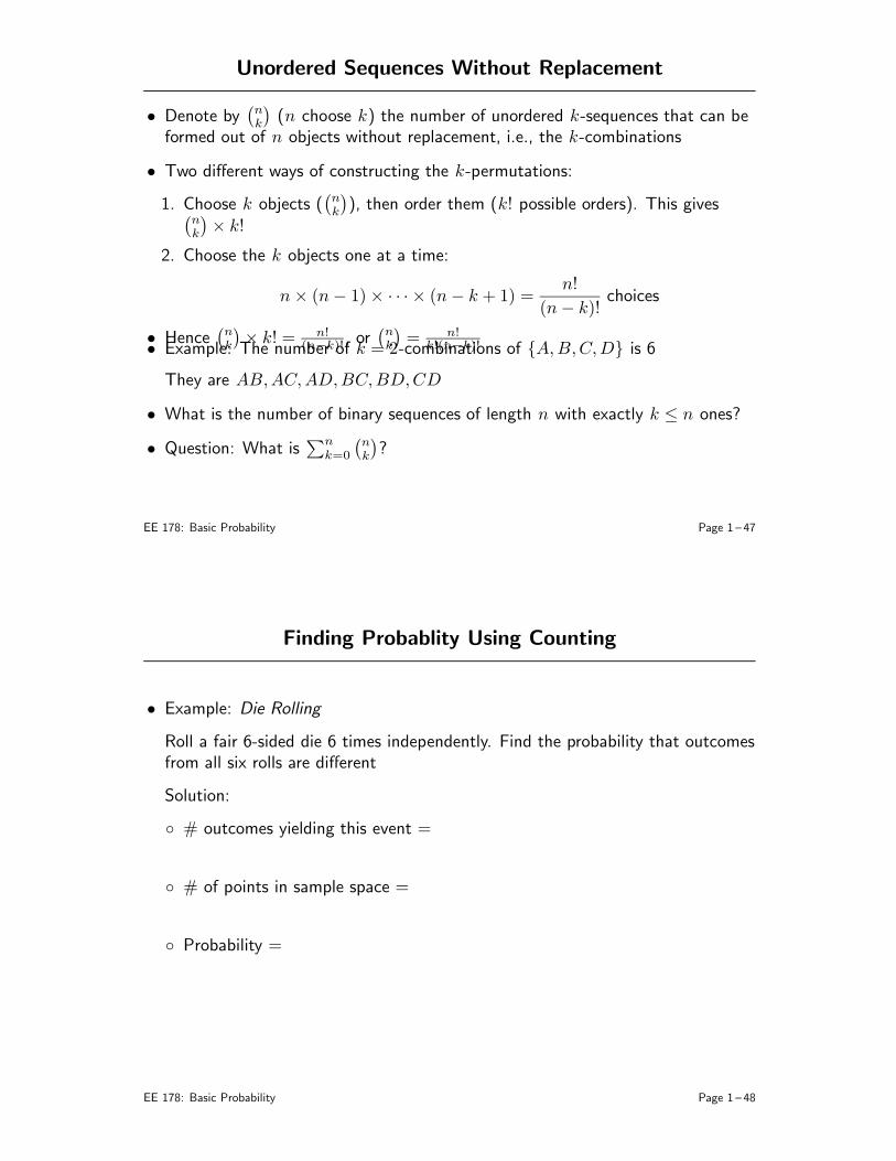
Unordered Sequences Without Replacement
• Denote by(
nk
)
(n choose k) the number of unordered k-sequences that can beformed out of n objects without replacement, i.e., the k-combinations
• Two different ways of constructing the k-permutations:
1. Choose k objects ((
nk
)
), then order them (k! possible orders). This gives(
nk
)
× k!
2. Choose the k objects one at a time:
n× (n− 1)× · · · × (n− k + 1) =n!
(n− k)!choices
• Hence(
nk
)
× k! = n!(n−k)! , or
(
nk
)
= n!k!(n−k)!• Example: The number of k = 2-combinations of A,B,C,D is 6
They are AB,AC,AD,BC,BD,CD
• What is the number of binary sequences of length n with exactly k ≤ n ones?
• Question: What is∑n
k=0
(
nk
)
?
EE 178: Basic Probability Page 1 – 47
Finding Probablity Using Counting
• Example: Die Rolling
Roll a fair 6-sided die 6 times independently. Find the probability that outcomesfrom all six rolls are different
Solution:
# outcomes yielding this event =
# of points in sample space =
Probability =
EE 178: Basic Probability Page 1 – 48

• Example: The Birthday Problem
k people are selected at random. What is the probability that all k birthdayswill be different (neglect leap years)
Solution:
Total # ways of assigning birthdays to k people:
# of ways of assigning birthdays to k people with no two having the samebirthday:
Probability:
EE 178: Basic Probability Page 1 – 49
Binomial Probabilities
• Consider n independent coin tosses, where P(H) = p for 0 < p < 1
• Outcome is a sequence of H s and T s of length n
P(sequence) = p#heads(1− p)#tails
• The probability of k heads in n tosses is thus
P(k heads) =∑
sequences with k heads
P(sequence)
= #(k−head sequences)× pk(1− p)n−k
=
(
n
k
)
pk(1− p)n−k
Check that it sums to 1
EE 178: Basic Probability Page 1 – 50

• Example: Toss a coin with bias p independently 10 times.
Define the events B = 3 out of 10 tosses are heads andA = first two tosses are heads. Find P(A|B)
Solution: The conditional probability is
P(A|B) =P(A,B)
P(B)
All points in B have the same probability p3(1− p)7, so we can find theconditional probability by counting:
# points in B beginning with two heads =
# points in B =
Probability =
EE 178: Basic Probability Page 1 – 51
Partitions
• Let n1, n2, n3, . . . , nr be such that
r∑
i=1
ni = n
How many ways can the n objects be partitioned into r subsets (unorderedsequences) with the ith subset having exactly ni objects?
• If r = 2 with n1, n− n1 the answer is the n1-combinations( (nn1)
)
• Answer in general:
EE 178: Basic Probability Page 1 – 52

(
n
n1 n2 . . . nr
)
=
(
n
n1
)
×
(
n− n1
n2
)
×
(
n− (n1 + n2)
n3
)
× . . .
(
n−∑r−1
i=1 ni
nr
)
=n!
n1!(n− n1)!×
(n− n1)!
n2!(n− (n1 + n2))!× · · ·
=n!
n1!n2! · · ·nr!
EE 178: Basic Probability Page 1 – 53
• Example: Balls and bins
We have n balls and r bins. We throw each ball independently and at randominto a bin. What is the probability that bin i = 1, 2, . . . , r will have exactly ni
balls, where∑r
i=1 ni = n?
Solution:
The probability of each outcome (sequence of ni balls in bin i) is:
# of ways of partitioning the n balls into r bins such that bin i has exactlyni balls is:
Probability:
EE 178: Basic Probability Page 1 – 54

• Example: Cards
Consider a perfectly shuffled 52-card deck dealt to 4 players. FindP(each player gets an ace)
Solution:
Size of the sample space is:
# of ways of distributing the four aces:
# of ways of dealing the remaining 48 cards:
Probability =
EE 178: Basic Probability Page 1 – 55

EE 178 Lecture Notes 1
Basic Probability
• Set Theory
• Elements of Probability
• Conditional probability
• Sequential Calculation of Probability
• Total Probability and Bayes Rule
• Independence
• Counting
EE 178: Basic Probability Page 1 – 1
Set Theory Basics
• A set is a collection of objects, which are its elements
ω ∈ A means that ω is an element of the set A
A set with no elements is called the empty set, denoted by ∅
• Types of sets:
Finite: A = ω1, ω2, . . . , ωn
Countably infinite: A = ω1, ω2, . . ., e.g., the set of integers
Uncountable: A set that takes a continuous set of values, e.g., the [0, 1]interval, the real line, etc.
• A set can be described by all ω having a certain property, e.g., A = [0, 1] can bewritten as A = ω : 0 ≤ ω ≤ 1
• A set B ⊂ A means that every element of B is an element of A
• A universal set Ω contains all objects of particular interest in a particularcontext, e.g., sample space for random experiment
EE 178: Basic Probability Page 1 – 2

Set Operations
• Assume a universal set Ω
• Three basic operations:
Complementation: A complement of a set A with respect to Ω isAc = ω ∈ Ω : ω /∈ A, so Ωc = ∅
Intersection: A ∩B = ω : ω ∈ A and ω ∈ B
Union: A ∪B = ω : ω ∈ A or ω ∈ B
• Notation:
∪ni=1Ai = A1 ∪A2 . . . ∪An
∩ni=1Ai = A1 ∩A2 . . . ∩An
• A collection of sets A1, A2, . . . , An are disjoint or mutually exclusive ifAi ∩Aj = ∅ for all i 6= j , i.e., no two of them have a common element
• A collection of sets A1, A2, . . . , An partition Ω if they are disjoint and∪ni=1Ai = Ω
EE 178: Basic Probability Page 1 – 3
• Venn Diagrams
(e) A ∩ B (f) A ∪ B
(b) A
(d) Bc
(a) Ω
(c) B
EE 178: Basic Probability Page 1 – 4

Algebra of Sets
• Basic relations:
1. S ∩ Ω = S
2. (Ac)c = A
3. A ∩Ac = ∅
4. Commutative law: A ∪B = B ∪A
5. Associative law: A ∪ (B ∪ C) = (A ∪B) ∪ C
6. Distributive law: A ∩ (B ∪ C) = (A ∩B) ∪ (A ∩ C)
7. DeMorgan’s law: (A ∩B)c = Ac ∪Bc
DeMorgan’s law can be generalized to n events:
(∩ni=1Ai)
c= ∪n
i=1Aci
• These can all be proven using the definition of set operations or visualized usingVenn Diagrams
EE 178: Basic Probability Page 1 – 5
Elements of Probability
• Probability theory provides the mathematical rules for assigning probabilities tooutcomes of random experiments, e.g., coin flips, packet arrivals, noise voltage
• Basic elements of probability:
Sample space: The set of all possible “elementary” or “finest grain”outcomes of the random experiment (also called sample points)– The sample points are all disjoint– The sample points are collectively exhaustive, i.e., together they make upthe entire sample space
Events: Subsets of the sample space
Probability law : An assignment of probabilities to events in a mathematicallyconsistent way
EE 178: Basic Probability Page 1 – 6
Discrete Sample Spaces
• Sample space is called discrete if it contains a countable number of samplepoints
• Examples:
Flip a coin once: Ω = H, T
Flip a coin three times: Ω = HHH,HHT,HTH, . . . = H,T3
Flip a coin n times: Ω = H,Tn (set of sequences of H and T of length n)
Roll a die once: Ω = 1, 2, 3, 4, 5, 6
Roll a die twice: Ω = (1, 1), (1, 2), (2, 1), . . . , (6, 6) = 1, 2, 3, 4, 5, 62
Flip a coin until the first heads appears: Ω = H,TH, TTH, TTTH, . . .
Number of packets arriving in time interval (0, T ] at a node in acommunication network : Ω = 0, 1, 2, 3, . . .
Note that the first five examples have finite Ω, whereas the last two havecountably infinite Ω. Both types are called discrete
EE 178: Basic Probability Page 1 – 7
• Sequential models: For sequential experiments, the sample space can bedescribed in terms of a tree, where each outcome corresponds to a terminalnode (or a leaf)
Example: Three flips of a coin
|
H
|
H
|
@@@@@@
T|
AAAAAAAAAAA
T
|
H
|
@@@@@@
T|
HHHHHHHT
HHHHHHHT
HHHHHHHT
HHHHHHHT
|HHH
|HHT
|HTH
|HTT
|THH
|THT
|TTH
|TTT
EE 178: Basic Probability Page 1 – 8

• Example: Roll a fair four-sided die twice.
Sample space can be represented by a tree as above, or graphically
f
f
f
f
f
f
f
f
f
f
f
f
f
f
f
f
2nd roll
1st roll
1
2
3
4
1 2 3 4
EE 178: Basic Probability Page 1 – 9
Continuous Sample Spaces
• A continuous sample space consists of a continuum of points and thus containsan uncountable number of points
• Examples:
Random number between 0 and 1: Ω = [0, 1]
Suppose we pick two numbers at random between 0 and 1, then the samplespace consists of all points in the unit square, i.e., Ω = [0, 1]2
6
-
1.0
1.0x
y
EE 178: Basic Probability Page 1 – 10

Packet arrival time: t ∈ (0,∞), thus Ω = (0,∞)
Arrival times for n packets: ti ∈ (0,∞), for i = 1, 2, . . . , n, thus Ω = (0,∞)n
• A sample space is said to be mixed if it is neither discrete nor continuous, e.g.,Ω = [0, 1] ∪ 3
EE 178: Basic Probability Page 1 – 11
Events
• Events are subsets of the sample space. An event occurs if the outcome of theexperiment belongs to the event
• Examples:
Any outcome (sample point) is an event (also called an elementary event),e.g., HTH in three coin flips experiment or 0.35 in the picking of arandom number between 0 and 1 experiment
Flip coin 3 times and get exactly one H. This is a more complicated event,consisting of three sample points TTH, THT, HTT
Flip coin 3 times and get an odd number of H’s. The event isTTH, THT, HTT, HHH
Pick a random number between 0 and 1 and get a number between 0.0 and0.5. The event is [0, 0.5]
• An event might have no points in it, i.e., be the empty set ∅
EE 178: Basic Probability Page 1 – 12

Axioms of Probability
• Probability law (measure or function) is an assignment of probabilities to events(subsets of sample space Ω) such that the following three axioms are satisfied:
1. P(A) ≥ 0, for all A (nonnegativity)
2. P(Ω) = 1 (normalization)
3. If A and B are disjoint (A ∩B = ∅), then
P(A ∪B) = P(A) + P(B) (additivity)
More generally,
3’. If the sample space has an infinite number of points and A1, A2, . . . aredisjoint events, then
P (∪∞
i=1Ai) =∞∑
i=1
P(Ai)
EE 178: Basic Probability Page 1 – 13
• Mimics relative frequency, i.e., perform the experiment n times (e.g., roll a die ntimes). If the number of occurances of A is nA, define the relative frequency ofan event A as fA = nA/n
Probabilities are nonnegative (like relative frequencies)
Probability something happens is 1 (again like relative frequencies)
Probabilities of disjoint events add (again like relative frequencies)
• Analogy: Except for normalization, probability is a measure much like
mass
length
area
volume
They all satisfy axioms 1 and 3
This analogy provides some intuition but is not sufficient to fully understandprobability theory — other aspects such as conditioning, independence, etc.., areunique to probability
EE 178: Basic Probability Page 1 – 14

Probability for Discrete Sample Spaces
• Recall that sample space Ω is said to be discrete if it is countable
• The probability measure P can be simply defined by first assigning probabilitiesto outcomes, i.e., elementary events ω, such that:
P(ω) ≥ 0, for all ω ∈ Ω, and∑
ω∈Ω
P(ω) = 1
• The probability of any other event A (by the additivity axiom) is simply
P(A) =∑
ω∈A
P(ω)
EE 178: Basic Probability Page 1 – 15
• Examples:
For the coin flipping experiment, assign
P(H) = p and P(T) = 1− p, for 0 ≤ p ≤ 1
Note: p is the bias of the coin, and a coin is fair if p = 12
For the die rolling experiment, assign
P(i) =1
6, for i = 1, 2, . . . , 6
The probability of the event “the outcome is even”, A = 2, 4, 6, is
P(A) = P(2) + P(4) + P(6) =1
2
EE 178: Basic Probability Page 1 – 16
If Ω is countably infinite, we can again assign probabilities to elementaryeventsExample: Assume Ω = 1, 2, . . ., assign probability 2−k to event kThe probability of the event “the outcome is even”
P( outcome is even ) = P(2, 4, 6, 8, . . .)
= P(2) + P(4) + P(6) + . . .
=∞∑
k=1
P(2k)
=∞∑
k=1
2−2k =1
3
EE 178: Basic Probability Page 1 – 17
Probability for Continuous Sample Space
• Recall that if a sample space is continuous, Ω is uncountably infinite
• For continuous Ω, we cannot in general define the probability measure P by firstassigning probabilities to outcomes
• To see why, consider assigning a uniform probability measure to Ω = (0, 1]
In this case the probability of each single outcome event is zero
How do we find the probability of an event such as A =[
12,
34
]
?
• For this example we can define uniform probability measure over [0, 1] byassigning to an event A, the probability
P(A) = length of A,
e.g., P([0, 1/3] ∪ [2/3, 1]) = 2/3
Check that this is a legitimate assignment
EE 178: Basic Probability Page 1 – 18
• Another example: Romeo and Juliet have a date. Each arrives late with arandom delay of up to 1 hour. Each will wait only 1/4 of an hour before leaving.What is the probability that Romeo and Juliet will meet?
Solution: The pair of delays is equivalent to that achievable by picking tworandom numbers between 0 and 1. Define probability of an event as its area
The event of interest is represented by the cross hatched region
6
-
1.0
1.0x
y
Probability of the event is:
area of crosshatched region = 1− 2×1
2(0.75)2 = 0.4375
EE 178: Basic Probability Page 1 – 19
Basic Properties of Probability
• There are several useful properties that can be derived from the axioms ofprobability:
1. P(Ac) = 1− P(A) P(∅) = 0 P(A) ≤ 1
2. If A ⊆ B , then P(A) ≤ P(B)
3. P(A ∪B) = P(A) + P(B)− P(A ∩ B)
4. P(A ∪B) ≤ P(A) + P(B), or in general
P(∪ni=1Ai) ≤
n∑
i=1
P(Ai)
This is called the Union of Events Bound
• These properties can be proved using the axioms of probability and visualizedusing Venn diagrams
EE 178: Basic Probability Page 1 – 20
Conditional Probability
• Conditional probability allows us to compute probabilities of events based onpartial knowledge of the outcome of a random experiment
• Examples:
We are told that the sum of the outcomes from rolling a die twice is 9. Whatis the probability the outcome of the first die was a 6?
A spot shows up on a radar screen. What is the probability that there is anaircraft?
You receive a 0 at the output of a digital communication system. What is theprobability that a 0 was sent?
• As we shall see, conditional probability provides us with two methods forcomputing probabilities of events: the sequential method and thedivide-and-conquer method
• It is also the basis of inference in statistics: make an observation and reasonabout the cause
EE 178: Basic Probability Page 1 – 21
• In general, given an event B has occurred, we wish to find the probability ofanother event A, P(A|B)
• If all elementary outcomes are equally likely, then
P(A|B) =# of outcomes in both A and B
# of outcomes in B
• In general, if B is an event such that P(B) 6= 0, the conditional probability ofany event A given B is defined as
P(A|B) =P(A ∩B)
P(B), or
P(A,B)
P(B)
• The function P(·|B) for fixed B specifies a probability law, i.e., it satisfies theaxioms of probability
EE 178: Basic Probability Page 1 – 22
Example
• Roll a fair four-sided die twice. So, the sample space is 1, 2, 3, 42. All samplepoints have probability 1/16
Let B be the event that the minimum of the two die rolls is 2 and Am, form = 1, 2, 3, 4, be the event that the maximum of the two die rolls is m. FindP(Am|B)
• Solution:
f
f
f
f
f
f
f
f
f
f
f
f
f
f
f
f
f
f
f
f f
2nd roll
1st roll
1
2
3
4
1 2 3 4
-
6
m
P(Am|B)
1 2 3 4
EE 178: Basic Probability Page 1 – 23
Conditional Probability Models
• Before: Probability law ⇒ conditional probabilities
• Reverse is often more natural: Conditional probabilities ⇒ probability law
• We use the chain rule (also called multiplication rule):
By the definition of conditional probability, P(A ∩B) = P(A|B)P(B). Supposethat A1, A2, . . . , An are events, then
EE 178: Basic Probability Page 1 – 24
P(A1 ∩A2 ∩A3 · · · ∩An)
= P(A1 ∩A2 ∩A3 · · · ∩An−1)× P(An|A1 ∩A2 ∩ A3 · · · ∩An−1)
= P(A1 ∩A2 ∩A3 · · · ∩An−2)× P(An−1|A1 ∩A2 ∩A3 · · · ∩An−2)
× P(An|A1 ∩A2 ∩A3 · · · ∩An−1)
...
= P(A1)× P(A2|A1)× P(A3|A1 ∩A2) · · ·P(An|A1 ∩A2 ∩A3 · · · ∩An−1)
=n∏
i=1
P(Ai|A1, A2, . . . , Ai−1),
where A0 = ∅
EE 178: Basic Probability Page 1 – 25
Sequential Calculation of Probabilities
• Procedure:
1. Construct a tree description of the sample space for a sequential experiment
2. Assign the conditional probabilities on the corresponding branches of the tree
3. By the chain rule, the probability of an outcome can be obtained bymultiplying the conditional probabilities along the path from the root to theleaf node corresponding to the outcome
• Example (Radar Detection): Let A be the event that an aircraft is flying aboveand B be the event that the radar detects it. Assume P(A) = 0.05,P(B|A) = 0.99, and P(B|Ac) = 0.1
What is the probability of
Missed detection?, i.e., P(A ∩ Bc)
False alarm?, i.e., P(B ∩Ac)
The sample space is: Ω = (A,B), (Ac, B), (A,Bc), (Ac, Bc)
EE 178: Basic Probability Page 1 – 26
Solution: Represent the sample space by a tree with conditional probabilities onits edges
P(A) = 0.05
P(B|A) = 0.99
@@@@@@
P(Bc|A) = 0.01
(A,B)
AAAAAAAAAAAA
P(Ac) = 0.95
P(B|Ac) = 0.10
(A,Bc) (Missed detection)
@@@@@@
P(Bc|Ac) = 0.90
(Ac, B) (False alarm)
(Ac, Bc)
EE 178: Basic Probability Page 1 – 27
Example: Three cards are drawn at random (without replacement) from a deckof cards. What is the probability of not drawing a heart?
Solution: Let Ai, i = 1, 2, 3, represent the event of no heart in the ith draw.We can represent the sample space as:
Ω = (A1, A2, A3), (Ac1, A2, A3), . . . , (A
c1, A
c2, A
c3)
To find the probability law, we represent the sample space by a tree, writeconditional probabilities on branches, and use the chain rule
EE 178: Basic Probability Page 1 – 28
~
P(A1) = 39/52
not heart~
P(A2|A1) = 38/51
(not heart, not heart)~
@@@@@@@
13/51
(not heart, heart)~
AAAAAAAAAAAAAA
P(Ac1) = 13/52
heart~
P(A3|A1, A2) = 37/50 (not heart, not heart, not heart)
HHHHHHH13/50 (not heart, not heart, heart)
~
~
EE 178: Basic Probability Page 1 – 29
Total probability – Divide and Conquer Method
• Let A1, A2, . . . , An be events that partition Ω, i.e., that are disjoint(Ai ∩Aj = ∅ for i 6= j) and ∪n
i=1Ai = Ω. Then for any event B
P(B) =n∑
i=1
P(Ai ∩B) =n∑
i=1
P(Ai)P(B|Ai)
This is called the Law of Total Probability. It also holds for n = ∞. It allows usto compute the probability of a complicated event from knowledge ofprobabilities of simpler events
• Example: Chess tournament, 3 types of opponents for a certain player.
P(Type 1) = 0.5, P(Win |Type1) = 0.3
P(Type 2) = 0.25, P(Win |Type2) = 0.4
P(Type 3) = 0.25, P(Win |Type3) = 0.5
What is probability of player winning?
EE 178: Basic Probability Page 1 – 30
Solution: Let B be the event of winning and Ai be the event of playing Type i,i = 1, 2, 3:
P(B) =3
∑
i=1
P(Ai)P(B|Ai)
= 0.5× 0.3 + 0.25× 0.4 + 0.25× 0.5
= 0.375
EE 178: Basic Probability Page 1 – 31
Bayes Rule
• Let A1, A2, . . . , An be nonzero probability events (the causes) that partition Ω,and let B be a nonzero probability event (the effect)
• We often know the a priori probabilities P(Ai), i = 1, 2, . . . , n and theconditional probabilities P(B|Ai)s and wish to find the a posteriori probabilities
P(Aj|B) for j = 1, 2, . . . , n
• From the definition of conditional probability, we know that
P(Aj|B) =P(B,Aj)
P(B)=
P(B|Aj)
P(B)P(Aj)
By the law of total probability
P(B) =n∑
i=1
P(Ai)P(B|Ai)
EE 178: Basic Probability Page 1 – 32

Substituting we obtain Bayes rule
P(Aj|B) =P(B|Aj)
∑ni=1P(Ai)P(B|Ai)
P(Aj) for j = 1, 2, . . . , n
• Bayes rule also applies when the number of events n = ∞
• Radar Example: Recall that A is event that the aircraft is flying above and B isthe event that the aircraft is detected by the radar. What is the probability thatan aircraft is actually there given that the radar indicates a detection?
Recall P(A) = 0.05, P(B|A) = 0.99, P(B|Ac) = 0.1. Using Bayes rule:
P(there is an aircraft|radar detects it) = P(A|B)
=P(B|A)P(A)
P(B|A)P(A) + P(B|Ac)P(Ac)
=0.05× 0.99
0.05× 0.99 + 0.95× 0.1
= 0.3426
EE 178: Basic Probability Page 1 – 33
Binary Communication Channel
• Consider a noisy binary communication channel, where 0 or 1 is sent and 0 or 1is received. Assume that 0 is sent with probability 0.2 (and 1 is sent withprobability 0.8)
The channel is noisy. If a 0 is sent, a 0 is received with probability 0.9, and if a1 is sent, a 1 is received with probability 0.975
• We can represent this channel model by a probability transition diagram
00
1 1
P(0|0) = 0.9
P(1|1) = 0.975
P(0) = 0.2
P(1) = 0.8
0.1
0.025
Given that 0 is received, find the probability that 0 was sent
EE 178: Basic Probability Page 1 – 34

• This is a random experiment with sample space Ω = (0, 0), (0, 1), (1, 0), (1, 1),where the first entry is the bit sent and the second is the bit received
• Define the two events
A = 0 is sent = (0, 1), (0, 0), and
B = 0 is received = (0, 0), (1, 0)
• The probability measure is defined via the P(A), P(B|A), and P(Bc|Ac)provided on the probability transition diagram of the channel
• To find P(A|B), the a posteriori probability that a 0 was sent. We use Bayesrule
P(A|B) =P(B|A)P(A)
P(A)P(B|A) + P(Ac)P(B|Ac),
to obtain
P(A|B) =0.9
0.2× 0.2 = 0.9,
which is much higher than the a priori probability of A (= 0.2)
EE 178: Basic Probability Page 1 – 35
Independence
• It often happens that the knowledge that a certain event B has occurred has noeffect on the probability that another event A has occurred, i.e.,
P(A|B) = P(A)
In this case we say that the two events are statistically independent
• Equivalently, two events are said to be statistically independent if
P(A,B) = P(A)P(B)
So, in this case, P(A|B) = P(A) and P(B|A) = P(B)
• Example: Assuming that the binary channel of the previous example is used tosend two bits independently, what is the probability that both bits are in error?
EE 178: Basic Probability Page 1 – 36

Solution:
Define the two events
E1 = First bit is in error
E2 = Second bit is in error
Since the bits are sent independently, the probability that both are in error is
P(E1, E2) = P(E1)P(E2)
Also by symmetry, P(E1) = P(E2)To find P(E1), we express E1 in terms of the events A and B as
E1 = (A1 ∩Bc1) ∪ (Ac
1 ∩B1),
EE 178: Basic Probability Page 1 – 37
Thus,
P(E1) = P(A1, Bc1) + P(Ac
1, B1)
= P(A1)P(Bc1|A1) + P(Ac
1)P(B1|Ac1)
= 0.2× 0.1 + 0.8× 0.025 = 0.04
The probability that the two bits are in error
P(E1, E2) = (0.04)2 = 16× 10−4
• In general A1, A2, . . . , An are mutually independent if for each subset of theevents Ai1, Ai2, . . . , Aik
P(Ai1, Ai2, . . . , Aik) =k∏
j=1
P(Aij)
• Note: P(A1, A2, . . . , An) =∏n
j=1P(Ai) alone is not sufficient for independence
EE 178: Basic Probability Page 1 – 38
Example: Roll two fair dice independently. Define the events
A = First die = 1, 2, or 3
B = First die = 2, 3, or 6
C = Sum of outcomes = 9
Are A, B , and C independent?
EE 178: Basic Probability Page 1 – 39
Solution:
Since the dice are fair and the experiments are performed independently, theprobability of any pair of outcomes is 1/36, and
P(A) =1
2, P(B) =
1
2, P(C) =
1
9
Since A ∩B ∩ C = (3, 6), P(A,B,C) = 136 = P(A)P(B)P(C)
But are A, B , and C independent? Let’s find
P(A,B) =2
6=
1
36=
1
4= P(A)P(B),
and thus A, B , and C are not independent!
EE 178: Basic Probability Page 1 – 40
• Also, independence of subsets does not necessarily imply independence
Example: Flip a fair coin twice independently. Define the events:
A: First toss is Head
B : Second toss is Head
C : First and second toss have different outcomes
A and B are independent, A and C are independent, and B and C areindependent
Are A,B,C mutually independent?
Clearly not, since if you know A and B , you know that C could not haveoccured, i.e., P(A,B,C) = 0 6= P(A)P(B)P(C) = 1/8
EE 178: Basic Probability Page 1 – 41
Counting
• Discrete uniform law:
Finite sample space where all sample points are equally probable:
P(A) =number of sample points in A
total number of sample points
Variation: all outcomes in A are equally likely, each with probability p. Then,
P(A) = p× (number of elements of A)
• In both cases, we compute probabilities by counting
EE 178: Basic Probability Page 1 – 42
Basic Counting Principle
• Procedure (multiplication rule):
r steps
ni choices at step i
Number of choices is n1 × n2 × · · · × nr
• Example:
Number of license plates with 3 letters followed by 4 digits:
With no repetition (replacement), the number is:
• Example: Consider a set of objects s1, s2, . . . , sn. How many subsets of theseobjects are there (including the set itself and the empty set)?
Each object may or may not be in the subset (2 options)
The number of subsets is:
EE 178: Basic Probability Page 1 – 43
De Mere’s Paradox
• Counting can be very tricky
• Classic example: Throw three 6-sided dice. Is the probability that the sum of theoutcomes is 11 equal to the the probability that the sum of the outcomes is 12?
• De Mere’s argued that they are, since the number of different ways to obtain 11and 12 are the same:
Sum=11: 6, 4, 1, 6, 3, 2, 5, 5, 1, 5, 4, 2, 5, 3, 3, 4, 4, 3
Sum=12: 6, 5, 1, 6, 4, 2, 6, 3, 3, 5, 5, 2, 5, 4, 3, 4, 4, 4
• This turned out to be false. Why?
EE 178: Basic Probability Page 1 – 44
Basic Types of Counting
• Assume we have n distinct objects a1, a2, . . . , an, e.g., digits, letters, etc.
• Some basic counting questions:
How many different ordered sequences of k objects can be formed out of then objects with replacement?
How many different ordered sequences of k ≤ n objects can be formed out ofthe n objects without replacement? (called k-permutations)
How many different unordered sequences (subsets) of k ≤ n objects can beformed out of the n objects without replacement? (called k-combinations)
Given r nonnegative integers n1, n2, . . . , nr that sum to n (the number ofobjects), how many ways can the n objects be partitioned into r subsets(unordered sequences) with the ith subset having exactly ni objects? (callerpartitions, and is a generalization of combinations)
EE 178: Basic Probability Page 1 – 45
Ordered Sequences With and Without Replacement
• The number of ordered k-sequences from n objects with replacement isn× n× n . . .× n k times, i.e., nk
Example: If n = 2, e.g., binary digits, the number of ordered k-sequences is 2k
• The number of different ordered sequences of k objects that can be formed fromn objects without replacement, i.e., the k-permutations, is
n× (n− 1)× (n− 2) · · · × (n− k + 1)
If k = n, the number is
n× (n− 1)× (n− 2) · · · × 2× 1 = n! (n-factorial)
Thus the number of k-permutations is: n!/(n− k)!
• Example: Consider the alphabet set A,B,C,D, so n = 4
The number of k = 2-permutations of n = 4 objects is 12
They are: AB,AC,AD,BA,BC,BD,CA,CB,CD,DA,DB, and DC
EE 178: Basic Probability Page 1 – 46

Unordered Sequences Without Replacement
• Denote by(
nk
)
(n choose k) the number of unordered k-sequences that can beformed out of n objects without replacement, i.e., the k-combinations
• Two different ways of constructing the k-permutations:
1. Choose k objects ((
nk
)
), then order them (k! possible orders). This gives(
nk
)
× k!
2. Choose the k objects one at a time:
n× (n− 1)× · · · × (n− k + 1) =n!
(n− k)!choices
• Hence(
nk
)
× k! = n!(n−k)! , or
(
nk
)
= n!k!(n−k)!• Example: The number of k = 2-combinations of A,B,C,D is 6
They are AB,AC,AD,BC,BD,CD
• What is the number of binary sequences of length n with exactly k ≤ n ones?
• Question: What is∑n
k=0
(
nk
)
?
EE 178: Basic Probability Page 1 – 47
Finding Probablity Using Counting
• Example: Die Rolling
Roll a fair 6-sided die 6 times independently. Find the probability that outcomesfrom all six rolls are different
Solution:
# outcomes yielding this event =
# of points in sample space =
Probability =
EE 178: Basic Probability Page 1 – 48
• Example: The Birthday Problem
k people are selected at random. What is the probability that all k birthdayswill be different (neglect leap years)
Solution:
Total # ways of assigning birthdays to k people:
# of ways of assigning birthdays to k people with no two having the samebirthday:
Probability:
EE 178: Basic Probability Page 1 – 49
Binomial Probabilities
• Consider n independent coin tosses, where P(H) = p for 0 < p < 1
• Outcome is a sequence of H s and T s of length n
P(sequence) = p#heads(1− p)#tails
• The probability of k heads in n tosses is thus
P(k heads) =∑
sequences with k heads
P(sequence)
= #(k−head sequences)× pk(1− p)n−k
=
(
n
k
)
pk(1− p)n−k
Check that it sums to 1
EE 178: Basic Probability Page 1 – 50
• Example: Toss a coin with bias p independently 10 times.
Define the events B = 3 out of 10 tosses are heads andA = first two tosses are heads. Find P(A|B)
Solution: The conditional probability is
P(A|B) =P(A,B)
P(B)
All points in B have the same probability p3(1− p)7, so we can find theconditional probability by counting:
# points in B beginning with two heads =
# points in B =
Probability =
EE 178: Basic Probability Page 1 – 51
Partitions
• Let n1, n2, n3, . . . , nr be such that
r∑
i=1
ni = n
How many ways can the n objects be partitioned into r subsets (unorderedsequences) with the ith subset having exactly ni objects?
• If r = 2 with n1, n− n1 the answer is the n1-combinations( (nn1)
)
• Answer in general:
EE 178: Basic Probability Page 1 – 52
(
n
n1 n2 . . . nr
)
=
(
n
n1
)
×
(
n− n1
n2
)
×
(
n− (n1 + n2)
n3
)
× . . .
(
n−∑r−1
i=1 ni
nr
)
=n!
n1!(n− n1)!×
(n− n1)!
n2!(n− (n1 + n2))!× · · ·
=n!
n1!n2! · · ·nr!
EE 178: Basic Probability Page 1 – 53
• Example: Balls and bins
We have n balls and r bins. We throw each ball independently and at randominto a bin. What is the probability that bin i = 1, 2, . . . , r will have exactly ni
balls, where∑r
i=1 ni = n?
Solution:
The probability of each outcome (sequence of ni balls in bin i) is:
# of ways of partitioning the n balls into r bins such that bin i has exactlyni balls is:
Probability:
EE 178: Basic Probability Page 1 – 54

• Example: Cards
Consider a perfectly shuffled 52-card deck dealt to 4 players. FindP(each player gets an ace)
Solution:
Size of the sample space is:
# of ways of distributing the four aces:
# of ways of dealing the remaining 48 cards:
Probability =
EE 178: Basic Probability Page 1 – 55
Lecture Notes 2
Random Variables
• Definition
• Discrete Random Variables: Probability mass function (pmf)
• Continuous Random Variables: Probability density function (pdf)
• Mean and Variance
• Cumulative Distribution Function (cdf)
• Functions of Random Variables
Corresponding pages from B&T textbook: 72–83, 86, 88, 90, 140–144, 146–150, 152–157, 179–186.
EE 178: Random Variables Page 2 – 1
Random Variable
• A random variable is a real-valued variable that takes on values randomlySounds nice, but not terribly precise or useful
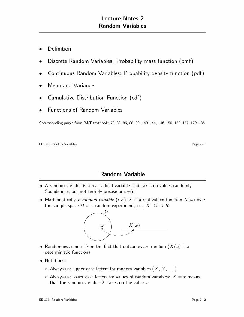
• Mathematically, a random variable (r.v.) X is a real-valued function X(ω) overthe sample space Ω of a random experiment, i.e., X : Ω → R
Ω
ω X(ω)
• Randomness comes from the fact that outcomes are random (X(ω) is adeterministic function)
• Notations:
Always use upper case letters for random variables (X , Y , . . .)
Always use lower case letters for values of random variables: X = x meansthat the random variable X takes on the value x
EE 178: Random Variables Page 2 – 2
• Examples:
1. Flip a coin n times. Here Ω = H,Tn. Define the random variableX ∈ 0, 1, 2, . . . , n to be the number of heads
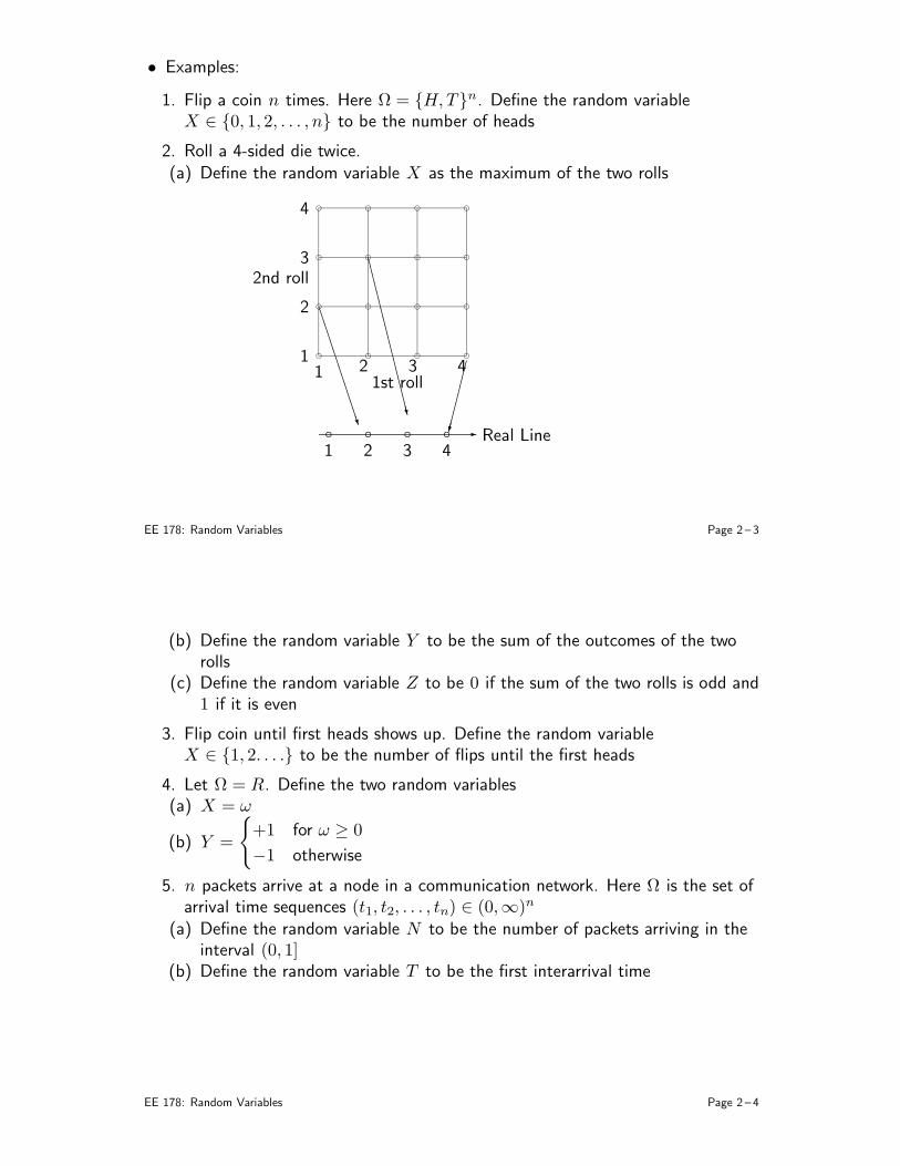
2. Roll a 4-sided die twice.(a) Define the random variable X as the maximum of the two rolls
e
e
e
e
e
e
e
e
e
e
e
e
e
e
e
e
2nd roll
1st roll
1
2
3
4
1 2 3 4
- Real Linee e e e
1 2 3 4
BBBBBBBBBBBBBBN
CCCCCCCCCCCCCCCCCCCW
EE 178: Random Variables Page 2 – 3
(b) Define the random variable Y to be the sum of the outcomes of the tworolls
(c) Define the random variable Z to be 0 if the sum of the two rolls is odd and1 if it is even
3. Flip coin until first heads shows up. Define the random variableX ∈ 1, 2. . . . to be the number of flips until the first heads
4. Let Ω = R. Define the two random variables(a) X = ω
(b) Y =
+1 for ω ≥ 0
−1 otherwise
5. n packets arrive at a node in a communication network. Here Ω is the set ofarrival time sequences (t1, t2, . . . , tn) ∈ (0,∞)n
(a) Define the random variable N to be the number of packets arriving in theinterval (0, 1]
(b) Define the random variable T to be the first interarrival time
EE 178: Random Variables Page 2 – 4
• Why do we need random variables?
Random variable can represent the gain or loss in a random experiment, e.g.,stock market
Random variable can represent a measurement over a random experiment,e.g., noise voltage on a resistor
• In most applications we care more about these costs/measurements than theunderlying probability space
• Very often we work directly with random variables without knowing (or caring toknow) the underlying probability space
EE 178: Random Variables Page 2 – 5
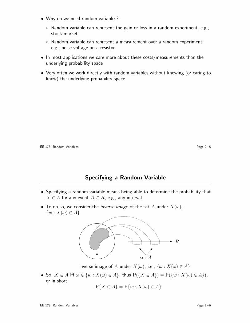
Specifying a Random Variable
• Specifying a random variable means being able to determine the probability thatX ∈ A for any event A ⊂ R, e.g., any interval
• To do so, we consider the inverse image of the set A under X(ω),w : X(ω) ∈ A
R
set A
inverse image of A under X(ω), i.e., ω : X(ω) ∈ A
• So, X ∈ A iff ω ∈ w : X(ω) ∈ A, thus P(X ∈ A) = P(w : X(ω) ∈ A),or in short
PX ∈ A = Pw : X(ω) ∈ A
EE 178: Random Variables Page 2 – 6
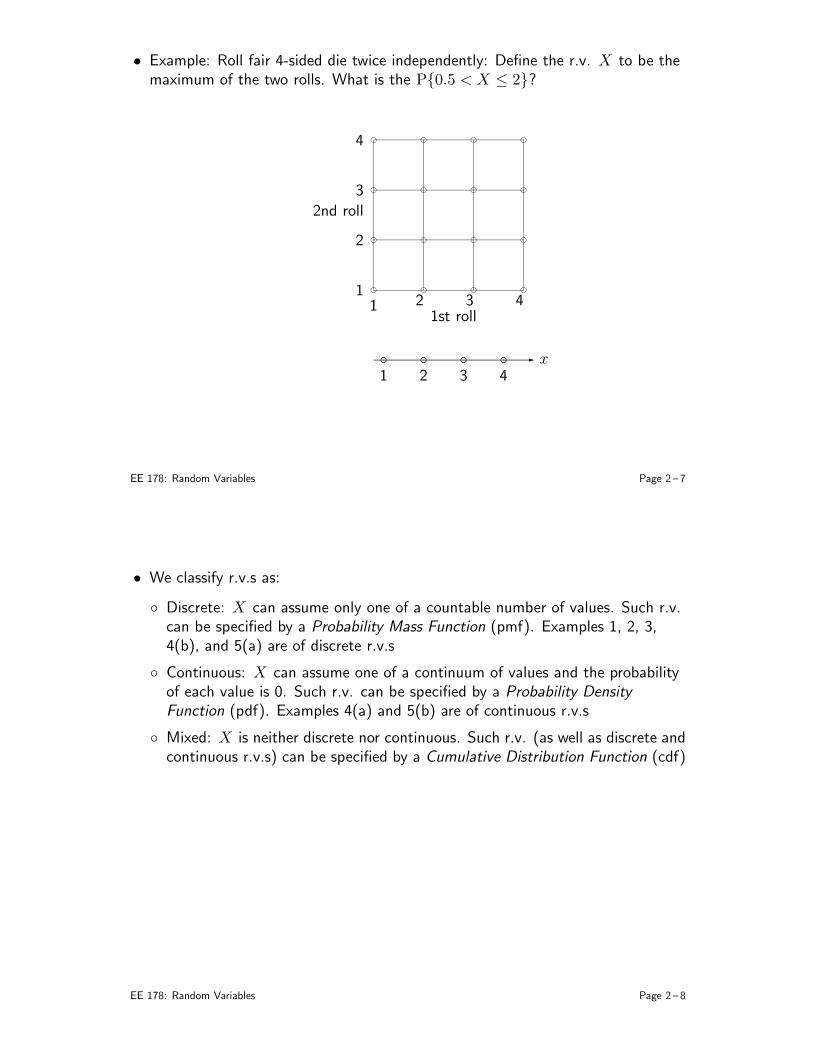
• Example: Roll fair 4-sided die twice independently: Define the r.v. X to be themaximum of the two rolls. What is the P0.5 < X ≤ 2?
f
f
f
f
f
f
f
f
f
f
f
f
f
f
f
f
2nd roll
1st roll
1
2
3
4
1 2 3 4
- xf f f f
1 2 3 4
EE 178: Random Variables Page 2 – 7
• We classify r.v.s as:
Discrete: X can assume only one of a countable number of values. Such r.v.can be specified by a Probability Mass Function (pmf). Examples 1, 2, 3,4(b), and 5(a) are of discrete r.v.s
Continuous: X can assume one of a continuum of values and the probabilityof each value is 0. Such r.v. can be specified by a Probability Density
Function (pdf). Examples 4(a) and 5(b) are of continuous r.v.s
Mixed: X is neither discrete nor continuous. Such r.v. (as well as discrete andcontinuous r.v.s) can be specified by a Cumulative Distribution Function (cdf)
EE 178: Random Variables Page 2 – 8
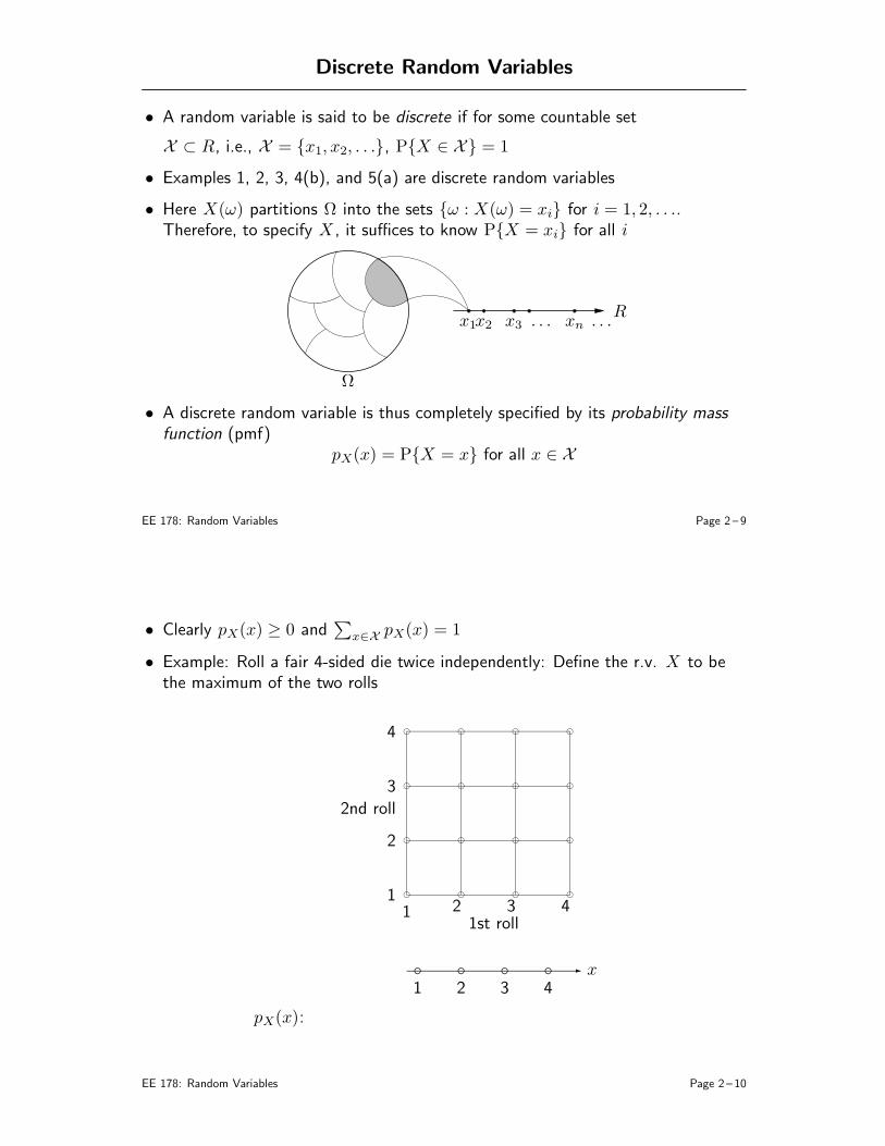
Discrete Random Variables
• A random variable is said to be discrete if for some countable set
X ⊂ R, i.e., X = x1, x2, . . ., PX ∈ X = 1
• Examples 1, 2, 3, 4(b), and 5(a) are discrete random variables
• Here X(ω) partitions Ω into the sets ω : X(ω) = xi for i = 1, 2, . . ..Therefore, to specify X , it suffices to know PX = xi for all i
Ω
. . .. . .x1x2 x3 xnR
• A discrete random variable is thus completely specified by its probability mass
function (pmf)pX(x) = PX = x for all x ∈ X
EE 178: Random Variables Page 2 – 9
• Clearly pX(x) ≥ 0 and∑
x∈XpX(x) = 1
• Example: Roll a fair 4-sided die twice independently: Define the r.v. X to bethe maximum of the two rolls
f
f
f
f
f
f
f
f
f
f
f
f
f
f
f
f
2nd roll
1st roll
1
2
3
4
1 2 3 4
- xf f f f
1 2 3 4
pX(x):
EE 178: Random Variables Page 2 – 10
• Note that pX(x) can be viewed as a probability measure over a discrete samplespace (even though the original sample space may be continuous as in examples4(b) and 5(a))
• The probability of any event A ⊂ R is given by
PX ∈ A =∑
x∈A∩X
pX(x)
For the previous example P1 < X ≤ 2.5 or X ≥ 3.5 =
• Notation: We use X ∼ pX(x) or simply X ∼ p(x) to mean that the discreterandom variable X has pmf pX(x) or p(x)
EE 178: Random Variables Page 2 – 11
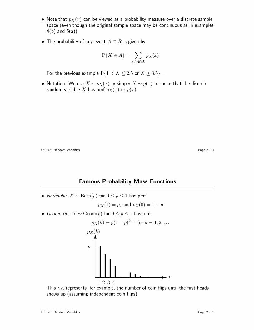
Famous Probability Mass Functions
• Bernoulli : X ∼ Bern(p) for 0 ≤ p ≤ 1 has pmf
pX(1) = p, and pX(0) = 1− p
• Geometric : X ∼ Geom(p) for 0 ≤ p ≤ 1 has pmf
pX(k) = p(1− p)k−1 for k = 1, 2, . . .
pX(k)
p
k1 2 3 4
. . .. . .
This r.v. represents, for example, the number of coin flips until the first headsshows up (assuming independent coin flips)
EE 178: Random Variables Page 2 – 12
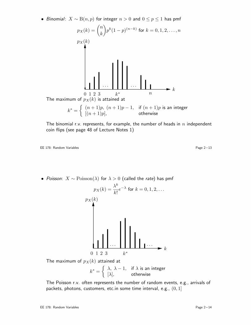
• Binomial : X ∼ B(n, p) for integer n > 0 and 0 ≤ p ≤ 1 has pmf
pX(k) =
(
n
k
)
pk(1− p)(n−k) for k = 0, 1, 2, . . . , n
pX(k)
k0 1 2 3
. . .. . .
nk∗
The maximum of pX(k) is attained at
k∗ =
(n+ 1)p, (n+ 1)p− 1, if (n+ 1)p is an integer[(n+ 1)p], otherwise
The binomial r.v. represents, for example, the number of heads in n independentcoin flips (see page 48 of Lecture Notes 1)
EE 178: Random Variables Page 2 – 13
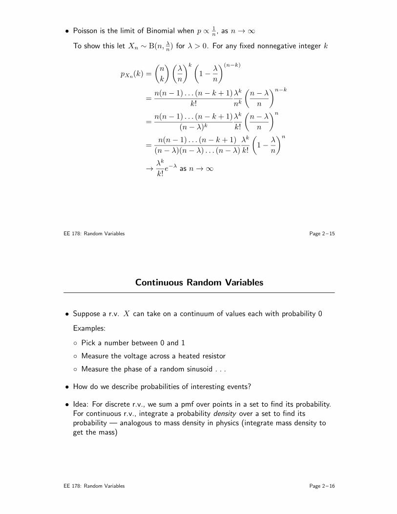
• Poisson: X ∼ Poisson(λ) for λ > 0 (called the rate) has pmf
pX(k) =λk
k!e−λ for k = 0, 1, 2, . . .
pX(k)
k1 2 30
. . . . . .
k∗
The maximum of pX(k) attained at
k∗ =
λ, λ− 1, if λ is an integer[λ], otherwise
The Poisson r.v. often represents the number of random events, e.g., arrivals ofpackets, photons, customers, etc.in some time interval, e.g., (0, 1]
EE 178: Random Variables Page 2 – 14
• Poisson is the limit of Binomial when p ∝ 1n , as n → ∞
To show this let Xn ∼ B(n, λn) for λ > 0. For any fixed nonnegative integer k
pXn(k) =
(
n
k
)(
λ
n
)k(
1−λ
n
)(n−k)
=n(n− 1) . . . (n− k + 1)
k!
λk
nk
(
n− λ
n
)n−k
=n(n− 1) . . . (n− k + 1)
(n− λ)kλk
k!
(
n− λ
n
)n
=n(n− 1) . . . (n− k + 1)
(n− λ)(n− λ) . . . (n− λ)
λk
k!
(
1−λ
n
)n
→λk
k!e−λ as n → ∞
EE 178: Random Variables Page 2 – 15
Continuous Random Variables
• Suppose a r.v. X can take on a continuum of values each with probability 0
Examples:
Pick a number between 0 and 1
Measure the voltage across a heated resistor
Measure the phase of a random sinusoid . . .
• How do we describe probabilities of interesting events?
• Idea: For discrete r.v., we sum a pmf over points in a set to find its probability.For continuous r.v., integrate a probability density over a set to find itsprobability — analogous to mass density in physics (integrate mass density toget the mass)
EE 178: Random Variables Page 2 – 16
Probability Density Function
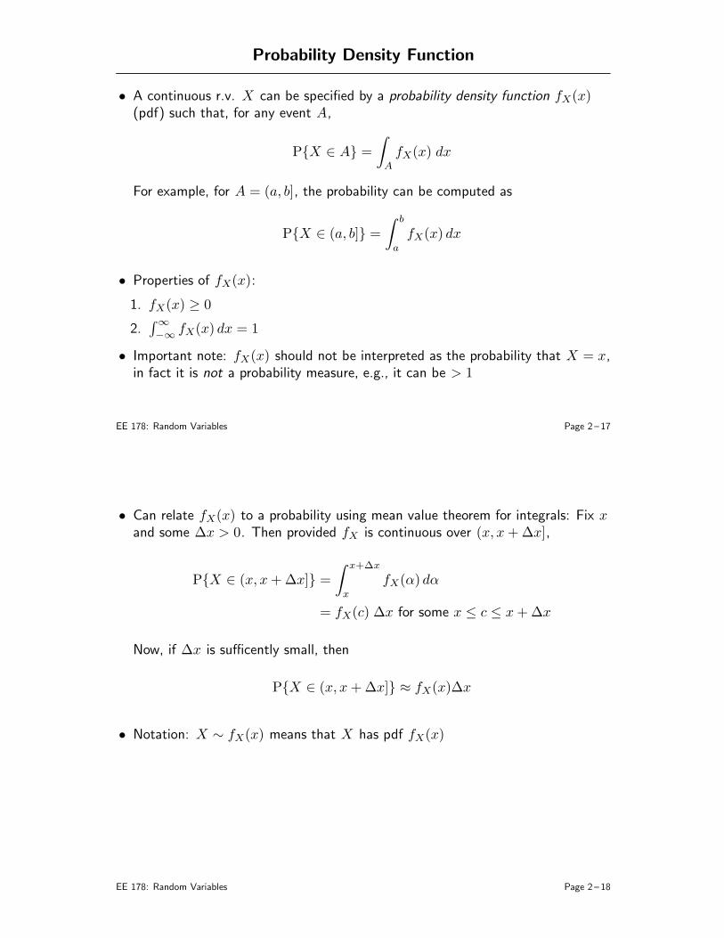
• A continuous r.v. X can be specified by a probability density function fX(x)(pdf) such that, for any event A,
PX ∈ A =
∫
A
fX(x) dx
For example, for A = (a, b], the probability can be computed as
PX ∈ (a, b] =
∫ b
a
fX(x) dx
• Properties of fX(x):
1. fX(x) ≥ 0
2.∫
∞
−∞fX(x) dx = 1
• Important note: fX(x) should not be interpreted as the probability that X = x,in fact it is not a probability measure, e.g., it can be > 1
EE 178: Random Variables Page 2 – 17
• Can relate fX(x) to a probability using mean value theorem for integrals: Fix xand some ∆x > 0. Then provided fX is continuous over (x, x+∆x],
PX ∈ (x, x+∆x] =
∫ x+∆x
x
fX(α) dα
= fX(c) ∆x for some x ≤ c ≤ x+∆x
Now, if ∆x is sufficently small, then
PX ∈ (x, x+∆x] ≈ fX(x)∆x
• Notation: X ∼ fX(x) means that X has pdf fX(x)
EE 178: Random Variables Page 2 – 18
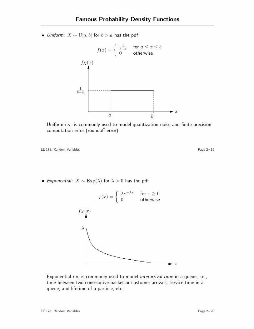
Famous Probability Density Functions
• Uniform: X ∼ U[a, b] for b > a has the pdf
f(x) =
1b−a for a ≤ x ≤ b
0 otherwise
fX(x)
1b−a
a bx
Uniform r.v. is commonly used to model quantization noise and finite precisioncomputation error (roundoff error)
EE 178: Random Variables Page 2 – 19
• Exponential : X ∼ Exp(λ) for λ > 0 has the pdf
f(x) =
λe−λx for x ≥ 00 otherwise
fX(x)
λ
x
Exponential r.v. is commonly used to model interarrival time in a queue, i.e.,time between two consecutive packet or customer arrivals, service time in aqueue, and lifetime of a particle, etc..
EE 178: Random Variables Page 2 – 20
Example: Let X ∼ Exp(0.1) be the customer service time at a bank (inminutes). The person ahead of you has been served for 5 minutes. What is theprobability that you will wait another 5 minutes or more before getting served?
We want to find PX > 10 |X > 5
Solution: By definition of conditional probability
PX > 10 |X > 5 =PX > 10, X > 5
PX > 5
=PX > 10
PX > 5
=
∫
∞
100.1e−0.1x dx
∫
∞
50.1e−0.1x dx
=e−1
e−0.5= e−0.5,
but PX > 5 = e−0.5, i.e., the conditional probability of waiting more than 5additional minutes given that you have already waited more than 5 minutes isthe same as the unconditional probability of waiting more than 5 minutes!
EE 178: Random Variables Page 2 – 21
This is because the exponential r.v. is memoryless, which in general means thatfor any 0 ≤ x1 < x,
PX > x |X > x1 = PX > x− x1
To show this, consider
PX > x |X > x1 =PX > x, X > x1
PX > x1
=PX > x
PX > x1
=
∫
∞
xλe−λx dx
∫
∞
x1λe−λx dx
=e−λx
e−λx1= e−λ(x−x1)
= PX > x− x1
EE 178: Random Variables Page 2 – 22
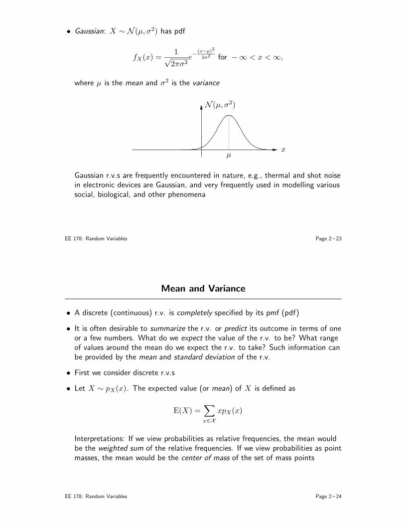
• Gaussian: X ∼ N (µ, σ2) has pdf
fX(x) =1
√2πσ2
e−
(x−µ)2
2σ2 for −∞ < x < ∞,
where µ is the mean and σ2 is the variance
N (µ, σ2)
µx
Gaussian r.v.s are frequently encountered in nature, e.g., thermal and shot noisein electronic devices are Gaussian, and very frequently used in modelling varioussocial, biological, and other phenomena
EE 178: Random Variables Page 2 – 23
Mean and Variance
• A discrete (continuous) r.v. is completely specified by its pmf (pdf)
• It is often desirable to summarize the r.v. or predict its outcome in terms of oneor a few numbers. What do we expect the value of the r.v. to be? What rangeof values around the mean do we expect the r.v. to take? Such information canbe provided by the mean and standard deviation of the r.v.
• First we consider discrete r.v.s
• Let X ∼ pX(x). The expected value (or mean) of X is defined as
E(X) =∑
x∈X
xpX(x)
Interpretations: If we view probabilities as relative frequencies, the mean wouldbe the weighted sum of the relative frequencies. If we view probabilities as pointmasses, the mean would be the center of mass of the set of mass points
EE 178: Random Variables Page 2 – 24
• Example: If the weather is good, which happens with probability 0.6, Alice walksthe 2 miles to class at a speed 5 miles/hr, otherwise she rides a bus at speed 30miles/hr. What is the expected time to get to class?
Solution: Define the discrete r.v. T to take the value (2/5)hr with probability0.6 and (2/30)hr with probability 0.4. The expected value of T
E(T ) = 2/5× 0.6 + 2/30× 0.4 = 4/15 hr
• The second moment (or mean square or average power) of X is defined as
E(X2) =∑
x∈X
x2pX(x)
For the previous example, the second moment is
E(T 2) = (2/5)2 × 0.6 + (2/30)2 × 0.4 = 22/225 hr2
• The variance of X is defined as
Var(X) = E[
(X − E(X))2]
=∑
x∈X
(x− E(X))2pX(x)
EE 178: Random Variables Page 2 – 25
Note that the Var ≥ 0. The variance has the interpretation of the moment of
inertia about the center of mass for a set of mass points
• The standard deviation of X is defined as σX =√
Var(X)
• Variance in terms of mean and second moment: Expanding the square and usingthe linearity of sum, we obtain
Var(X) = E[
(X − E(X))2]
=∑
x
(x− E(X))2pX(x)
=∑
x
(x2 − 2xE(X) + [E(X)]2)pX(x)
=∑
x
x2pX(x)− 2E(X)∑
x
xpX(x) + [E(X)]2∑
x
pX(x)
= E(X2)− 2[E(X)]2 + [E(X)]2
= E(X2)− [E(X)]2
Note that since for any r.v., Var(X) ≥ 0, E(X2) ≥ (E(X))2
So, for our example, Var(T ) = 22/225− (4/15)2 = 0.02667.
EE 178: Random Variables Page 2 – 26
Mean and Variance of Famous Discrete RVs
• Bernoulli r.v. X ∼ Bern(p): The mean is
E(X) = p× 1 + (1− p)× 0 = p
The second moment is
E(X2) = p× 12 + (1− p)× 02 = p
Thus the variance is
Var(X) = E(X2)− (E(X))2 = p− p2 = p(1− p)
• Binomial r.v. X ∼ B(n, p): It is not easy to find it using the definition. Laterwe use a much simpler method to show that
E(X) = np
Var(X) = np(1− p)
Just n times the mean (variance) of a Bernoulli!
EE 178: Random Variables Page 2 – 27
• Geometric r.v. X ∼ Geom(p): The mean is
E(X) =∞∑
k=1
kp(1− p)k−1
=p
1− p
∞∑
k=1
k(1− p)k
=p
1− p
∞∑
k=0
k(1− p)k
=p
1− p×
1− p
p2=
1
p
Note: We found the series sum using the following trick:
Recall that for |a| < 1, the sum of the geometric series
∞∑
k=0
ak =1
1− a
EE 178: Random Variables Page 2 – 28
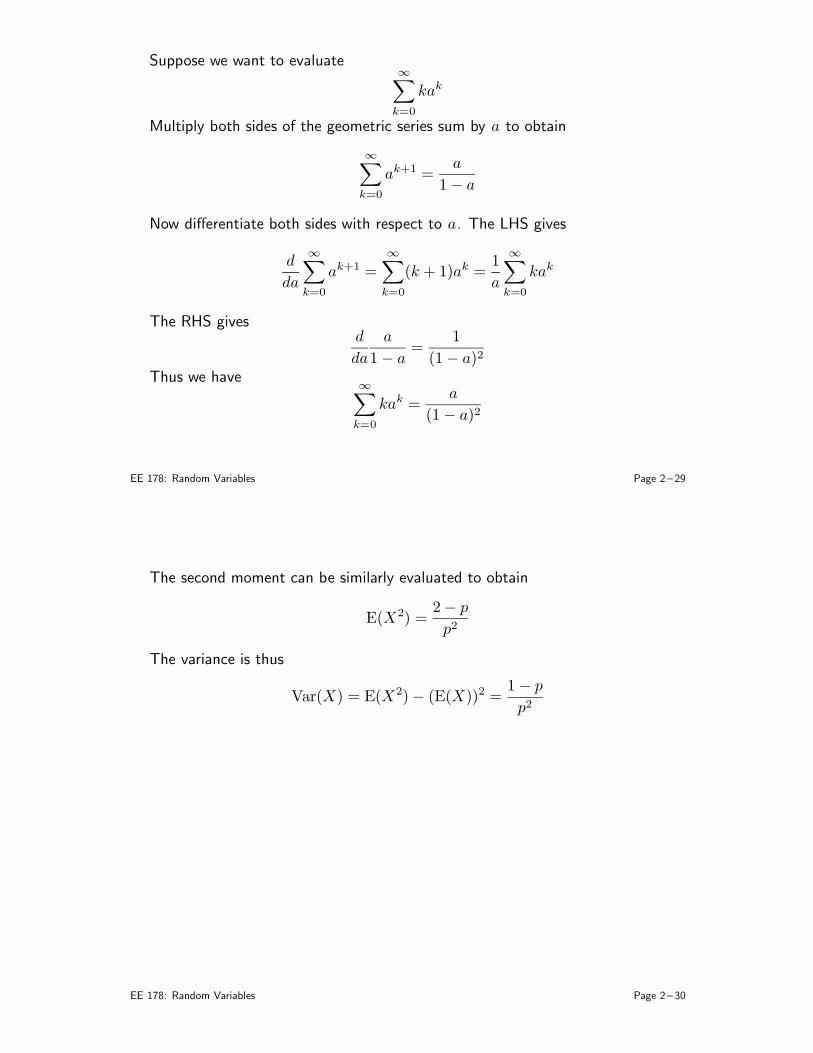
Suppose we want to evaluate∞∑
k=0
kak
Multiply both sides of the geometric series sum by a to obtain
∞∑
k=0
ak+1 =a
1− a
Now differentiate both sides with respect to a. The LHS gives
d
da
∞∑
k=0
ak+1 =∞∑
k=0
(k + 1)ak =1
a
∞∑
k=0
kak
The RHS givesd
da
a
1− a=
1
(1− a)2
Thus we have∞∑
k=0
kak =a
(1− a)2
EE 178: Random Variables Page 2 – 29
The second moment can be similarly evaluated to obtain
E(X2) =2− p
p2
The variance is thus
Var(X) = E(X2)− (E(X))2 =1− p
p2
EE 178: Random Variables Page 2 – 30
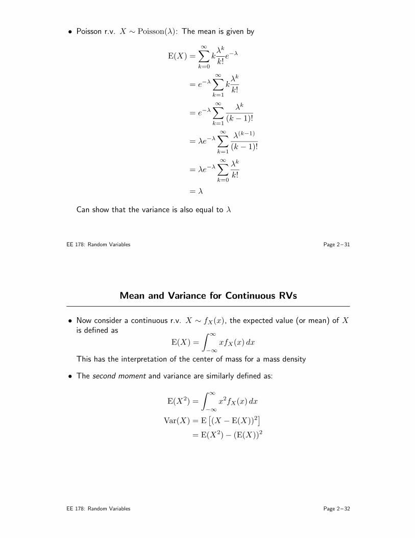
• Poisson r.v. X ∼ Poisson(λ): The mean is given by
E(X) =∞∑
k=0
kλk
k!e−λ
= e−λ∞∑
k=1
kλk
k!
= e−λ∞∑
k=1
λk
(k − 1)!
= λe−λ∞∑
k=1
λ(k−1)
(k − 1)!
= λe−λ∞∑
k=0
λk
k!
= λ
Can show that the variance is also equal to λ
EE 178: Random Variables Page 2 – 31
Mean and Variance for Continuous RVs
• Now consider a continuous r.v. X ∼ fX(x), the expected value (or mean) of Xis defined as
E(X) =
∫
∞
−∞
xfX(x) dx
This has the interpretation of the center of mass for a mass density
• The second moment and variance are similarly defined as:
E(X2) =
∫
∞
−∞
x2fX(x) dx
Var(X) = E[
(X − E(X))2]
= E(X2)− (E(X))2
EE 178: Random Variables Page 2 – 32
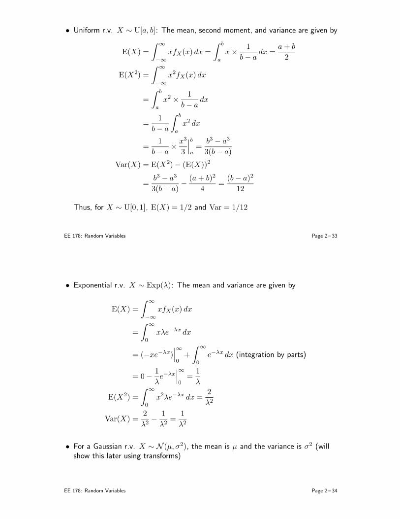
• Uniform r.v. X ∼ U[a, b]: The mean, second moment, and variance are given by
E(X) =
∫
∞
−∞
xfX(x) dx =
∫ b
a
x×1
b− adx =
a+ b
2
E(X2) =
∫
∞
−∞
x2fX(x) dx
=
∫ b
a
x2 ×1
b− adx
=1
b− a
∫ b
a
x2 dx
=1
b− a×
x3
3
∣
∣
∣
b
a=
b3 − a3
3(b− a)
Var(X) = E(X2)− (E(X))2
=b3 − a3
3(b− a)−
(a+ b)2
4=
(b− a)2
12
Thus, for X ∼ U[0, 1], E(X) = 1/2 and Var = 1/12
EE 178: Random Variables Page 2 – 33
• Exponential r.v. X ∼ Exp(λ): The mean and variance are given by
E(X) =
∫
∞
−∞
xfX(x) dx
=
∫
∞
0
xλe−λx dx
= (−xe−λx)∣
∣
∣
∞
0+
∫
∞
0
e−λx dx (integration by parts)
= 0−1
λe−λx
∣
∣
∣
∞
0=
1
λ
E(X2) =
∫
∞
0
x2λe−λx dx =2
λ2
Var(X) =2
λ2−
1
λ2=
1
λ2
• For a Gaussian r.v. X ∼ N (µ, σ2), the mean is µ and the variance is σ2 (willshow this later using transforms)
EE 178: Random Variables Page 2 – 34
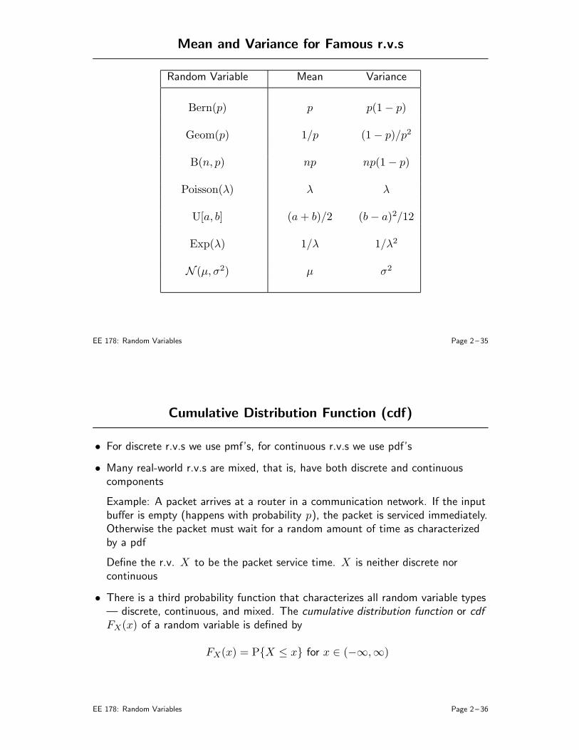
Mean and Variance for Famous r.v.s
Random Variable Mean Variance
Bern(p) p p(1− p)
Geom(p) 1/p (1− p)/p2
B(n, p) np np(1− p)
Poisson(λ) λ λ
U[a, b] (a+ b)/2 (b− a)2/12
Exp(λ) 1/λ 1/λ2
N (µ, σ2) µ σ2
EE 178: Random Variables Page 2 – 35
Cumulative Distribution Function (cdf)
• For discrete r.v.s we use pmf’s, for continuous r.v.s we use pdf’s
• Many real-world r.v.s are mixed, that is, have both discrete and continuouscomponents
Example: A packet arrives at a router in a communication network. If the inputbuffer is empty (happens with probability p), the packet is serviced immediately.Otherwise the packet must wait for a random amount of time as characterizedby a pdf
Define the r.v. X to be the packet service time. X is neither discrete norcontinuous
• There is a third probability function that characterizes all random variable types— discrete, continuous, and mixed. The cumulative distribution function or cdfFX(x) of a random variable is defined by
FX(x) = PX ≤ x for x ∈ (−∞,∞)
EE 178: Random Variables Page 2 – 36
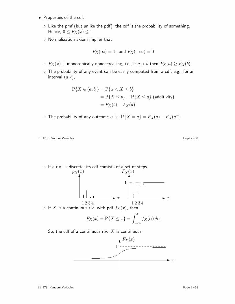
• Properties of the cdf:
Like the pmf (but unlike the pdf), the cdf is the probability of something.Hence, 0 ≤ FX(x) ≤ 1
Normalization axiom implies that
FX(∞) = 1, and FX(−∞) = 0
FX(x) is monotonically nondecreasing, i.e., if a > b then FX(a) ≥ FX(b)
The probability of any event can be easily computed from a cdf, e.g., for aninterval (a, b],
PX ∈ (a, b] = Pa < X ≤ b
= PX ≤ b − PX ≤ a (additivity)
= FX(b)− FX(a)
The probability of any outcome a is: PX = a = FX(a)− FX(a−)
EE 178: Random Variables Page 2 – 37
If a r.v. is discrete, its cdf consists of a set of stepspX(x) FX(x)
x x
1
11 22 33 44 If X is a continuous r.v. with pdf fX(x), then
FX(x) = PX ≤ x =
∫ x
−∞
fX(α) dα
So, the cdf of a continuous r.v. X is continuous
FX(x)
1
x
EE 178: Random Variables Page 2 – 38
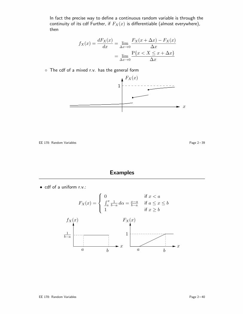
In fact the precise way to define a continuous random variable is through thecontinuity of its cdf Further, if FX(x) is differentiable (almost everywhere),then
fX(x) =dFX(x)
dx= lim
∆x→0
FX(x+∆x)− FX(x)
∆x
= lim∆x→0
Px < X ≤ x+∆x
∆x
The cdf of a mixed r.v. has the general form
FX(x)
1
x
EE 178: Random Variables Page 2 – 39
Examples
• cdf of a uniform r.v.:
FX(x) =
0 if x < a∫ x
a1
b−a dα = x−ab−a if a ≤ x ≤ b
1 if x ≥ b
fX(x) FX(x)
1b−a
a a bbxx
1
EE 178: Random Variables Page 2 – 40
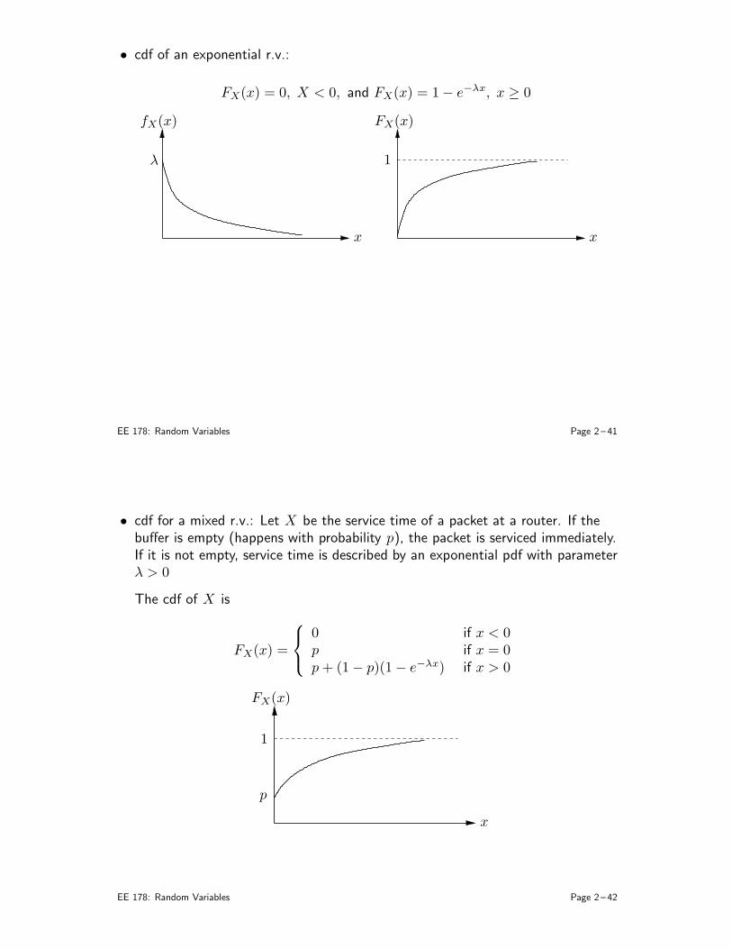
• cdf of an exponential r.v.:
FX(x) = 0, X < 0, and FX(x) = 1− e−λx, x ≥ 0
fX(x) FX(x)
λ 1
xx
EE 178: Random Variables Page 2 – 41
• cdf for a mixed r.v.: Let X be the service time of a packet at a router. If thebuffer is empty (happens with probability p), the packet is serviced immediately.If it is not empty, service time is described by an exponential pdf with parameterλ > 0
The cdf of X is
FX(x) =
0 if x < 0p if x = 0p+ (1− p)(1− e−λx) if x > 0
FX(x)
p
1
x
EE 178: Random Variables Page 2 – 42
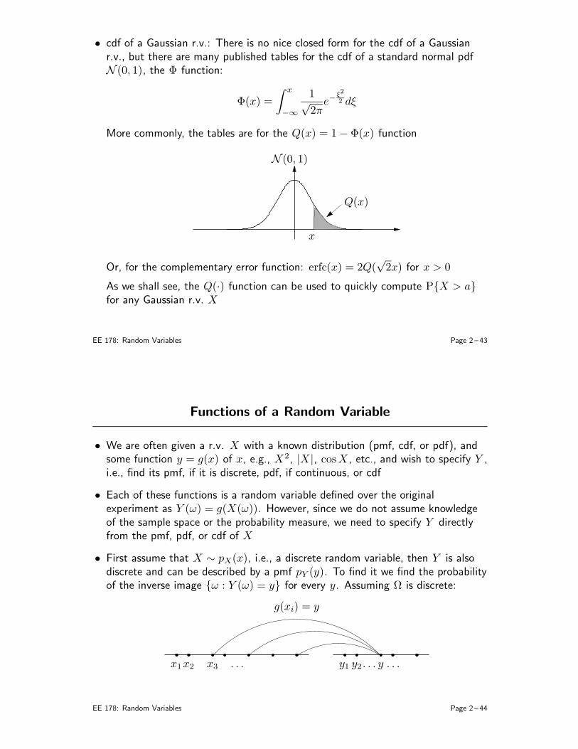
• cdf of a Gaussian r.v.: There is no nice closed form for the cdf of a Gaussianr.v., but there are many published tables for the cdf of a standard normal pdfN (0, 1), the Φ function:
Φ(x) =
∫ x
−∞
1√2π
e−ξ2
2 dξ
More commonly, the tables are for the Q(x) = 1− Φ(x) function
N (0, 1)
x
Q(x)
Or, for the complementary error function: erfc(x) = 2Q(√2x) for x > 0
As we shall see, the Q(·) function can be used to quickly compute PX > afor any Gaussian r.v. X
EE 178: Random Variables Page 2 – 43
Functions of a Random Variable
• We are often given a r.v. X with a known distribution (pmf, cdf, or pdf), andsome function y = g(x) of x, e.g., X2, |X |, cosX , etc., and wish to specify Y ,i.e., find its pmf, if it is discrete, pdf, if continuous, or cdf
• Each of these functions is a random variable defined over the originalexperiment as Y (ω) = g(X(ω)). However, since we do not assume knowledgeof the sample space or the probability measure, we need to specify Y directlyfrom the pmf, pdf, or cdf of X
• First assume that X ∼ pX(x), i.e., a discrete random variable, then Y is alsodiscrete and can be described by a pmf pY (y). To find it we find the probabilityof the inverse image ω : Y (ω) = y for every y. Assuming Ω is discrete:
x1x2 x3 y1 y2 y . . .. . .. . .
g(xi) = y
EE 178: Random Variables Page 2 – 44
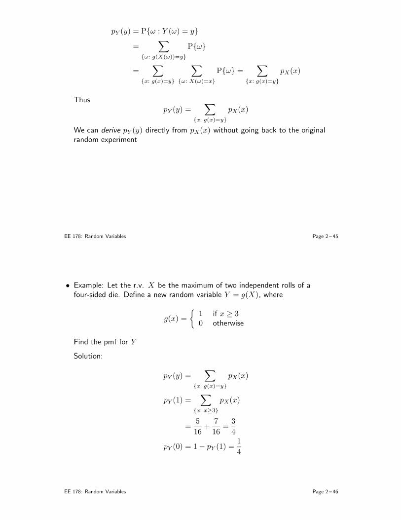
pY (y) = Pω : Y (ω) = y
=∑
ω: g(X(ω))=y
Pω
=∑
x: g(x)=y
∑
ω: X(ω)=x
Pω =∑
x: g(x)=y
pX(x)
ThuspY (y) =
∑
x: g(x)=y
pX(x)
We can derive pY (y) directly from pX(x) without going back to the originalrandom experiment
EE 178: Random Variables Page 2 – 45
• Example: Let the r.v. X be the maximum of two independent rolls of afour-sided die. Define a new random variable Y = g(X), where
g(x) =
1 if x ≥ 30 otherwise
Find the pmf for Y
Solution:
pY (y) =∑
x: g(x)=y
pX(x)
pY (1) =∑
x: x≥3
pX(x)
=5
16+
7
16=
3
4
pY (0) = 1− pY (1) =1
4
EE 178: Random Variables Page 2 – 46
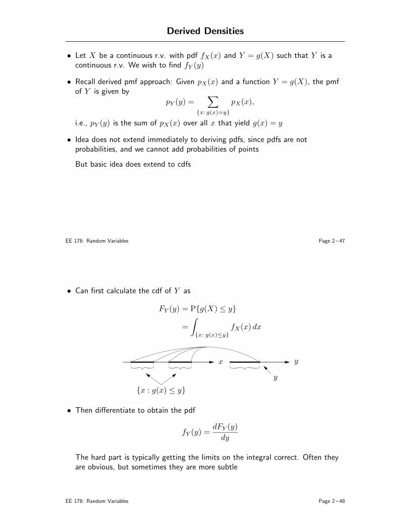
Derived Densities
• Let X be a continuous r.v. with pdf fX(x) and Y = g(X) such that Y is acontinuous r.v. We wish to find fY (y)
• Recall derived pmf approach: Given pX(x) and a function Y = g(X), the pmfof Y is given by
pY (y) =∑
x: g(x)=y
pX(x),
i.e., pY (y) is the sum of pX(x) over all x that yield g(x) = y
• Idea does not extend immediately to deriving pdfs, since pdfs are notprobabilities, and we cannot add probabilities of points
But basic idea does extend to cdfs
EE 178: Random Variables Page 2 – 47
• Can first calculate the cdf of Y as
FY (y) = Pg(X) ≤ y
=
∫
x: g(x)≤y
fX(x) dx
x y
y
x : g(x) ≤ y
• Then differentiate to obtain the pdf
fY (y) =dFY (y)
dy
The hard part is typically getting the limits on the integral correct. Often theyare obvious, but sometimes they are more subtle
EE 178: Random Variables Page 2 – 48
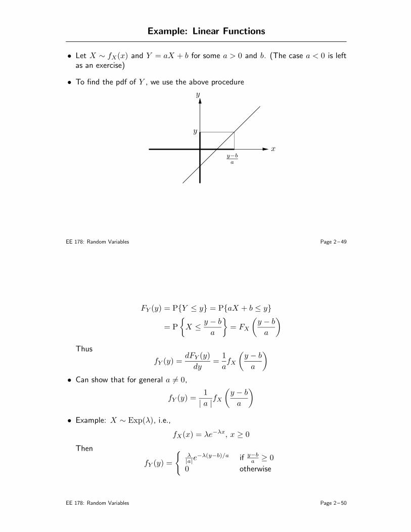
Example: Linear Functions
• Let X ∼ fX(x) and Y = aX + b for some a > 0 and b. (The case a < 0 is leftas an exercise)
• To find the pdf of Y , we use the above procedure
y
x
y
y−ba
EE 178: Random Variables Page 2 – 49
FY (y) = PY ≤ y = PaX + b ≤ y
= P
X ≤y − b
a
= FX
(
y − b
a
)
Thus
fY (y) =dFY (y)
dy=
1
afX
(
y − b
a
)
• Can show that for general a 6= 0,
fY (y) =1
| a |fX
(
y − b
a
)
• Example: X ∼ Exp(λ), i.e.,
fX(x) = λe−λx, x ≥ 0
Then
fY (y) =
λ|a|e
−λ(y−b)/a if y−ba ≥ 0
0 otherwise
EE 178: Random Variables Page 2 – 50
• Example: X ∼ N (µ, σ2), i.e.,
fX(x) =1
√2πσ2
e−
(x−µ)2
2σ2
Again setting Y = aX + b,
fY (y) =1
| a |fX
(
y − b
a
)
=1
| a |
1√2πσ2
e−
(
y−ba −µ
)2
2σ2
=1
√
2π(aσ)2e−
(y−b−aµ)2
2a2σ2
=1
√
2πσ2Y
e−
(y−µY )2
2σ2Y for −∞ < y < ∞
Therefore, Y ∼ N (aµ+ b, a2σ2)
EE 178: Random Variables Page 2 – 51
This result can be used to compute probabilities for an arbitrary Gaussian r.v.from knowledge of the distribution a N (0, 1) r.v.
Suppose Y ∼ N (µY , σ2Y ) and we wish to find PY > y
From the above result, we can express Y = σYX + µY , where X ∼ N (0, 1)
Thus
PY > y = PσYX + µY > y
= P
X >y − µY
σY
= Q
(
y − µY
σY
)
EE 178: Random Variables Page 2 – 52
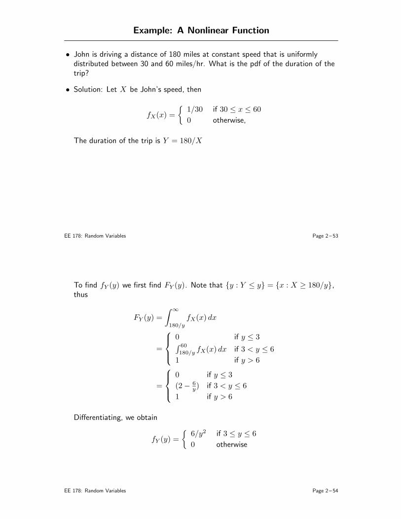
Example: A Nonlinear Function
• John is driving a distance of 180 miles at constant speed that is uniformlydistributed between 30 and 60 miles/hr. What is the pdf of the duration of thetrip?
• Solution: Let X be John’s speed, then
fX(x) =
1/30 if 30 ≤ x ≤ 60
0 otherwise,
The duration of the trip is Y = 180/X
EE 178: Random Variables Page 2 – 53
To find fY (y) we first find FY (y). Note that y : Y ≤ y = x : X ≥ 180/y,thus
FY (y) =
∫
∞
180/y
fX(x) dx
=
0 if y ≤ 3∫ 60
180/yfX(x) dx if 3 < y ≤ 6
1 if y > 6
=
0 if y ≤ 3
(2− 6y) if 3 < y ≤ 6
1 if y > 6
Differentiating, we obtain
fY (y) =
6/y2 if 3 ≤ y ≤ 6
0 otherwise
EE 178: Random Variables Page 2 – 54
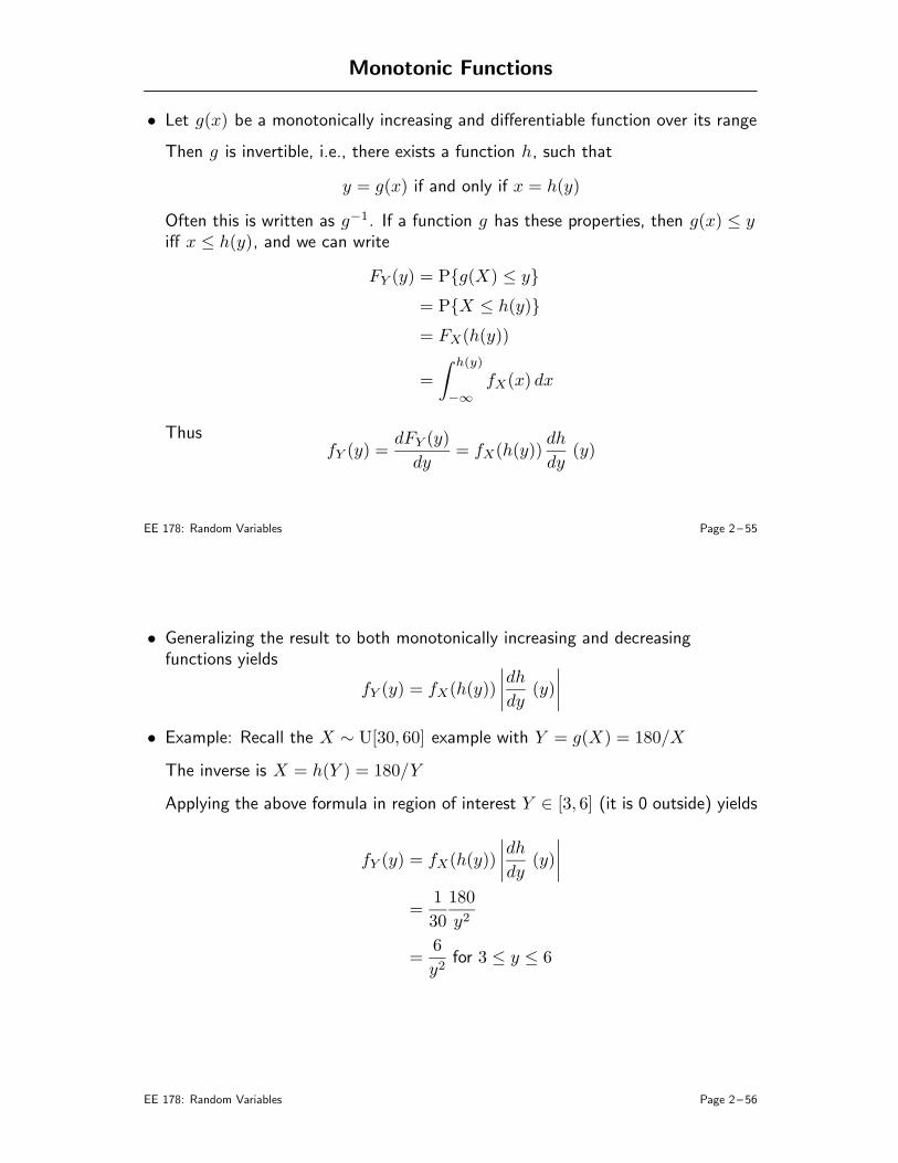
Monotonic Functions
• Let g(x) be a monotonically increasing and differentiable function over its range
Then g is invertible, i.e., there exists a function h, such that
y = g(x) if and only if x = h(y)
Often this is written as g−1. If a function g has these properties, then g(x) ≤ yiff x ≤ h(y), and we can write
FY (y) = Pg(X) ≤ y
= PX ≤ h(y)
= FX(h(y))
=
∫ h(y)
−∞
fX(x) dx
ThusfY (y) =
dFY (y)
dy= fX(h(y))
dh
dy(y)
EE 178: Random Variables Page 2 – 55
• Generalizing the result to both monotonically increasing and decreasingfunctions yields
fY (y) = fX(h(y))
∣
∣
∣
∣
dh
dy(y)
∣
∣
∣
∣
• Example: Recall the X ∼ U[30, 60] example with Y = g(X) = 180/X
The inverse is X = h(Y ) = 180/Y
Applying the above formula in region of interest Y ∈ [3, 6] (it is 0 outside) yields
fY (y) = fX(h(y))
∣
∣
∣
∣
dh
dy(y)
∣
∣
∣
∣
=1
30
180
y2
=6
y2for 3 ≤ y ≤ 6
EE 178: Random Variables Page 2 – 56
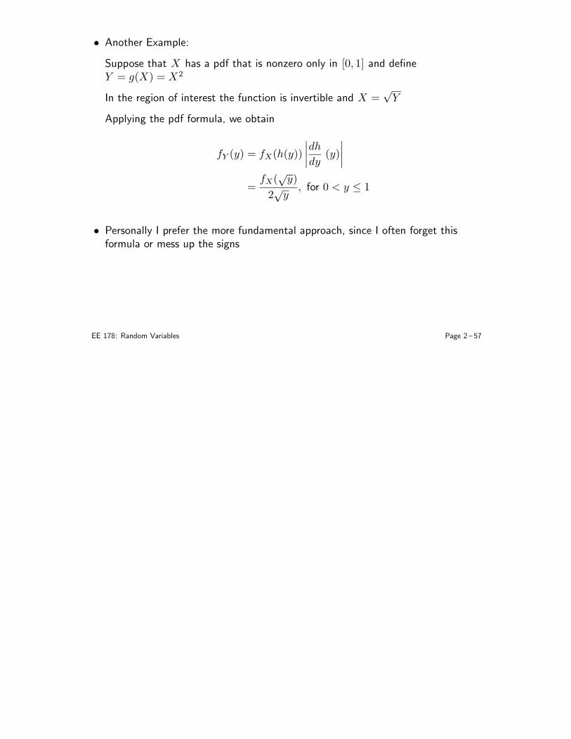
• Another Example:
Suppose that X has a pdf that is nonzero only in [0, 1] and defineY = g(X) = X2
In the region of interest the function is invertible and X =√Y
Applying the pdf formula, we obtain
fY (y) = fX(h(y))
∣
∣
∣
∣
dh
dy(y)
∣
∣
∣
∣
=fX(
√y)
2√y
, for 0 < y ≤ 1
• Personally I prefer the more fundamental approach, since I often forget thisformula or mess up the signs
EE 178: Random Variables Page 2 – 57
EE 178 Lecture Notes 3
Multiple Random Variables
• Joint, Marginal, and Conditional pmfs
• Bayes Rule and Independence for pmfs
• Joint, Marginal, and Conditional pdfs
• Bayes Rule and Independence for pdfs
• Functions of Two RVs
• One Discrete and One Continuous RVs
• More Than Two Random Variables
Corresponding pages from B&T textbook: 110-111, 158-159, 164-170, 173-178, 186-190, 221-225.
EE 178: Multiple Random Variables Page 3 – 1
Two Discrete Random Variables – Joint PMFs
• As we have seen, one can define several r.v.s on the sample space of a randomexperiment. How do we jointly specify multiple r.v.s, i.e., be able to determinethe probability of any event involving multiple r.v.s?
• We first consider two discrete r.v.s
• Let X and Y be two discrete random variables defined on the same experiment.They are completely specified by their joint pmf
pX,Y (x, y) = PX = x, Y = y for all x ∈ X , y ∈ Y
• Clearly, pX,Y (x, y) ≥ 0, and∑
x∈X
∑
y∈YpX,Y (x, y) = 1
• Notation: We use (X,Y ) ∼ pX,Y (x, y) to mean that the two discrete r.v.s havethe specified joint pmf
EE 178: Multiple Random Variables Page 3 – 2
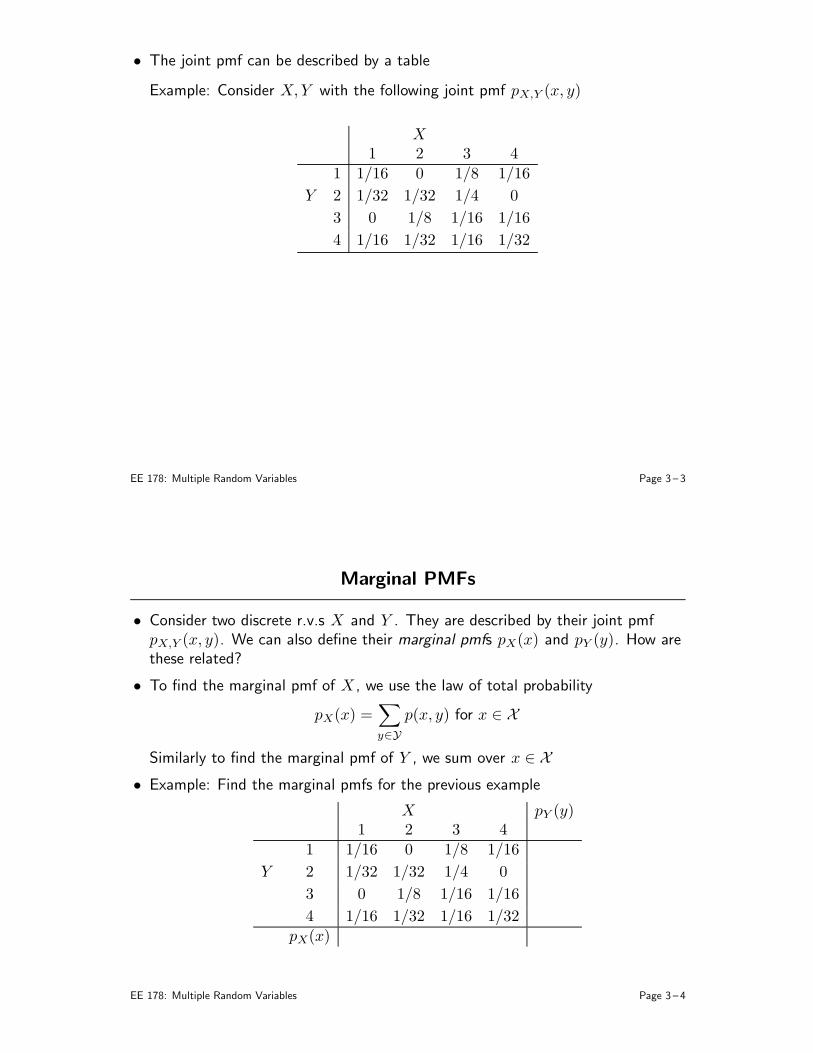
• The joint pmf can be described by a table
Example: Consider X,Y with the following joint pmf pX,Y (x, y)
X1 2 3 4
1 1/16 0 1/8 1/16
Y 2 1/32 1/32 1/4 0
3 0 1/8 1/16 1/16
4 1/16 1/32 1/16 1/32
EE 178: Multiple Random Variables Page 3 – 3
Marginal PMFs
• Consider two discrete r.v.s X and Y . They are described by their joint pmfpX,Y (x, y). We can also define their marginal pmfs pX(x) and pY (y). How arethese related?
• To find the marginal pmf of X , we use the law of total probability
pX(x) =∑
y∈Y
p(x, y) for x ∈ X
Similarly to find the marginal pmf of Y , we sum over x ∈ X
• Example: Find the marginal pmfs for the previous example
X pY (y)1 2 3 4
1 1/16 0 1/8 1/16
Y 2 1/32 1/32 1/4 0
3 0 1/8 1/16 1/16
4 1/16 1/32 1/16 1/32pX(x)
EE 178: Multiple Random Variables Page 3 – 4
Conditional PMFs
• The conditional pmf of X given Y = y is defined as
pX|Y (x|y) =pX,Y (x, y)
pY (y)for pY (y) 6= 0 and x ∈ X
Also, the conditional pmf of Y given X = x is
pY |X(y|x) =pX,Y (x, y)
pX(x)for pX(x) 6= 0 and y ∈ Y
• For fixed x, pY |X(y|x) is a pmf for Y
• Example: Find pY |X(y|2) for the previous example
EE 178: Multiple Random Variables Page 3 – 5
• Chain rule: Can write
pX,Y (x, y) = pX(x)pY |X(y|x)
• Bayes rule for pmfs: Given pX(x) and pY |X(y|x) for all (x, y) ∈ X × Y , we canfind
pX|Y (x|y) =pX,Y (x, y)
pY (y)
=pY |X(y|x)
pY (y)pX(x)
=pY |X(y|x)
∑
x′∈X
pX,Y (x′, y)pX(x), by total probability
Using the chain rule, we obtain another version of Bayes rule
pX|Y (x|y) =pY |X(y|x)
∑
x′∈X
pX(x′)pY |X(y|x′)pX(x)
EE 178: Multiple Random Variables Page 3 – 6
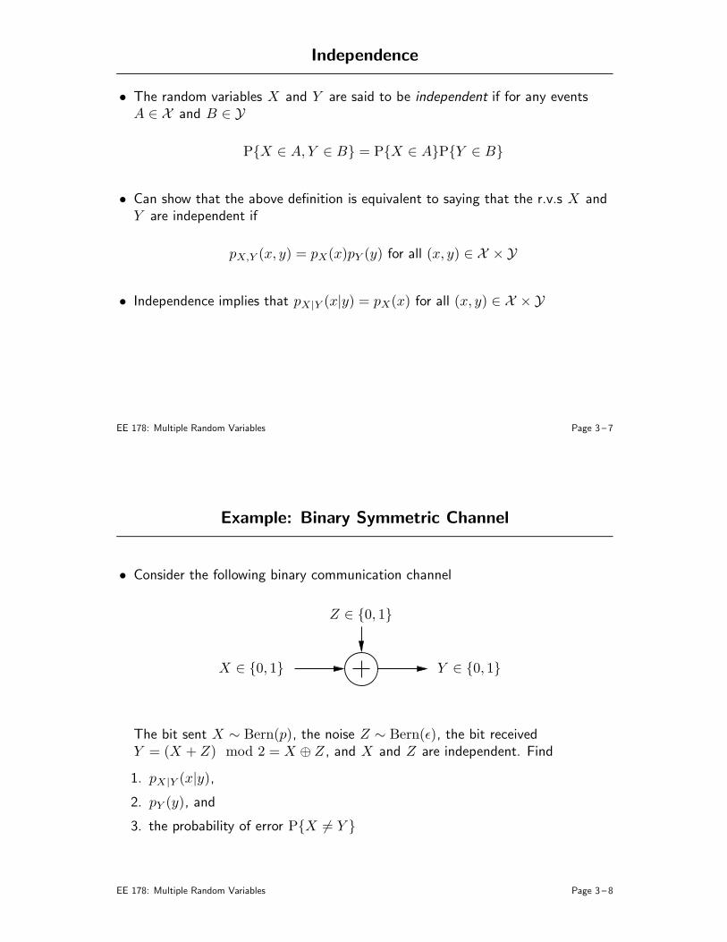
Independence
• The random variables X and Y are said to be independent if for any eventsA ∈ X and B ∈ Y
PX ∈ A, Y ∈ B = PX ∈ APY ∈ B
• Can show that the above definition is equivalent to saying that the r.v.s X andY are independent if
pX,Y (x, y) = pX(x)pY (y) for all (x, y) ∈ X × Y
• Independence implies that pX|Y (x|y) = pX(x) for all (x, y) ∈ X × Y
EE 178: Multiple Random Variables Page 3 – 7
Example: Binary Symmetric Channel
• Consider the following binary communication channel
X ∈ 0, 1 Y ∈ 0, 1
Z ∈ 0, 1
The bit sent X ∼ Bern(p), the noise Z ∼ Bern(ǫ), the bit receivedY = (X + Z) mod 2 = X ⊕ Z , and X and Z are independent. Find
1. pX|Y (x|y),
2. pY (y), and
3. the probability of error PX 6= Y
EE 178: Multiple Random Variables Page 3 – 8
1. To find pX|Y (x|y) we use Bayes rule
pX|Y (x|y) =pY |X(y|x)
∑
x′∈X
pY |X(y|x′)pX(x′)pX(x)
We know pX(x). To find pY |X , note that
pY |X(y|x) = PY = y|X = x
= PX ⊕ Z = y|X = x
= PZ = y ⊕X |X = x
= PZ = y ⊕ x|X = x
= PZ = y ⊕ x, since Z and X are independent
= pZ(y ⊕ x)
So we have
pY |X(0|0) = pZ(0⊕ 0) = pZ(0) = 1− ǫ, pY |X(0|1) = pZ(0⊕ 1) = pZ(1) = ǫ
pY |X(1|0) = pZ(1⊕ 0) = pZ(1) = ǫ, pY |X(1|1) = pZ(1⊕ 1) = pZ(0) = 1− ǫ
EE 178: Multiple Random Variables Page 3 – 9
Plugging in the Bayes rule equation, we obtain
pX|Y (0|0) =pY |X(0|0)
pY |X(0|0)pX(0) + pY |X(0|1)pX(1)pX(0)
=(1− ǫ)(1− p)
(1− ǫ)(1− p) + ǫp
pX|Y (1|0) =pY |X(0|1)
pY |X(0|0)pX(0) + pY |X(0|1)pX(1)pX(1) = 1− pX|Y (0|0)
=ǫp
(1− ǫ)(1− p) + ǫp
pX|Y (0|1) =pY |X(1|0)
pY |X(1|0)pX(0) + pY |X(1|1)pX(1)pX(0)
=ǫ(1− p)
ǫ(1− p) + (1− ǫ)p
pX|Y (1|1) =pY |X(1|1)
pY |X(1|0)pX(0) + pY |X(1|1)pX(1)pX(1) = 1− pX|Y (0|1)
=(1− ǫ)p
ǫ(1− p) + (1− ǫ)p
EE 178: Multiple Random Variables Page 3 – 10
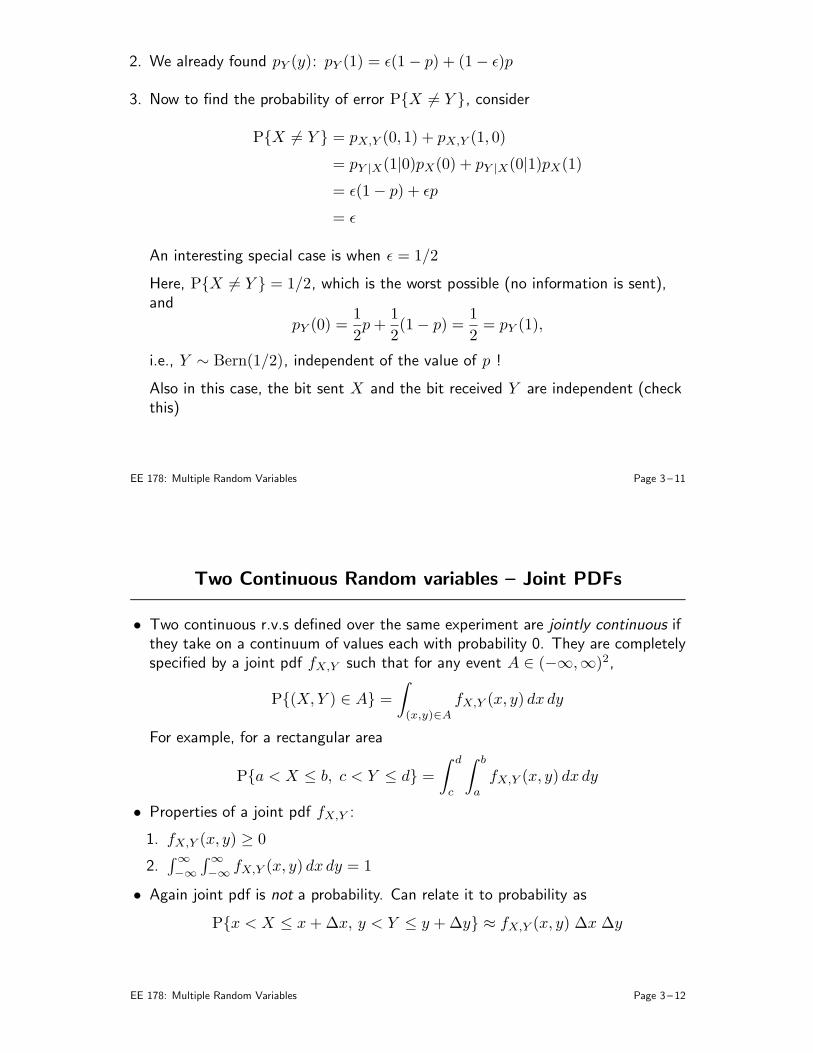
2. We already found pY (y): pY (1) = ǫ(1− p) + (1− ǫ)p
3. Now to find the probability of error PX 6= Y , consider
PX 6= Y = pX,Y (0, 1) + pX,Y (1, 0)
= pY |X(1|0)pX(0) + pY |X(0|1)pX(1)
= ǫ(1− p) + ǫp
= ǫ
An interesting special case is when ǫ = 1/2
Here, PX 6= Y = 1/2, which is the worst possible (no information is sent),and
pY (0) =1
2p+
1
2(1− p) =
1
2= pY (1),
i.e., Y ∼ Bern(1/2), independent of the value of p !
Also in this case, the bit sent X and the bit received Y are independent (checkthis)
EE 178: Multiple Random Variables Page 3 – 11
Two Continuous Random variables – Joint PDFs
• Two continuous r.v.s defined over the same experiment are jointly continuous ifthey take on a continuum of values each with probability 0. They are completelyspecified by a joint pdf fX,Y such that for any event A ∈ (−∞,∞)2,
P(X,Y ) ∈ A =
∫
(x,y)∈A
fX,Y (x, y) dx dy
For example, for a rectangular area
Pa < X ≤ b, c < Y ≤ d =
∫ d
c
∫ b
a
fX,Y (x, y) dx dy
• Properties of a joint pdf fX,Y :
1. fX,Y (x, y) ≥ 0
2.∫
∞
−∞
∫
∞
−∞fX,Y (x, y) dx dy = 1
• Again joint pdf is not a probability. Can relate it to probability as
Px < X ≤ x+∆x, y < Y ≤ y +∆y ≈ fX,Y (x, y) ∆x ∆y
EE 178: Multiple Random Variables Page 3 – 12
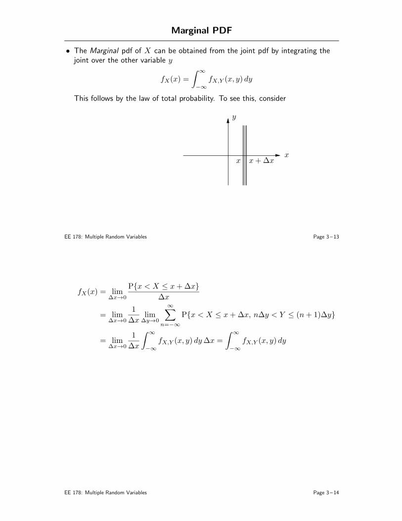
Marginal PDF
• The Marginal pdf of X can be obtained from the joint pdf by integrating thejoint over the other variable y
fX(x) =
∫
∞
−∞
fX,Y (x, y) dy
This follows by the law of total probability. To see this, consider
x
y
x x+∆x
EE 178: Multiple Random Variables Page 3 – 13
fX(x) = lim∆x→0
Px < X ≤ x+∆x
∆x
= lim∆x→0
1
∆xlim
∆y→0
∞∑
n=−∞
Px < X ≤ x+∆x, n∆y < Y ≤ (n+ 1)∆y
= lim∆x→0
1
∆x
∫
∞
−∞
fX,Y (x, y) dy∆x =
∫
∞
−∞
fX,Y (x, y) dy
EE 178: Multiple Random Variables Page 3 – 14
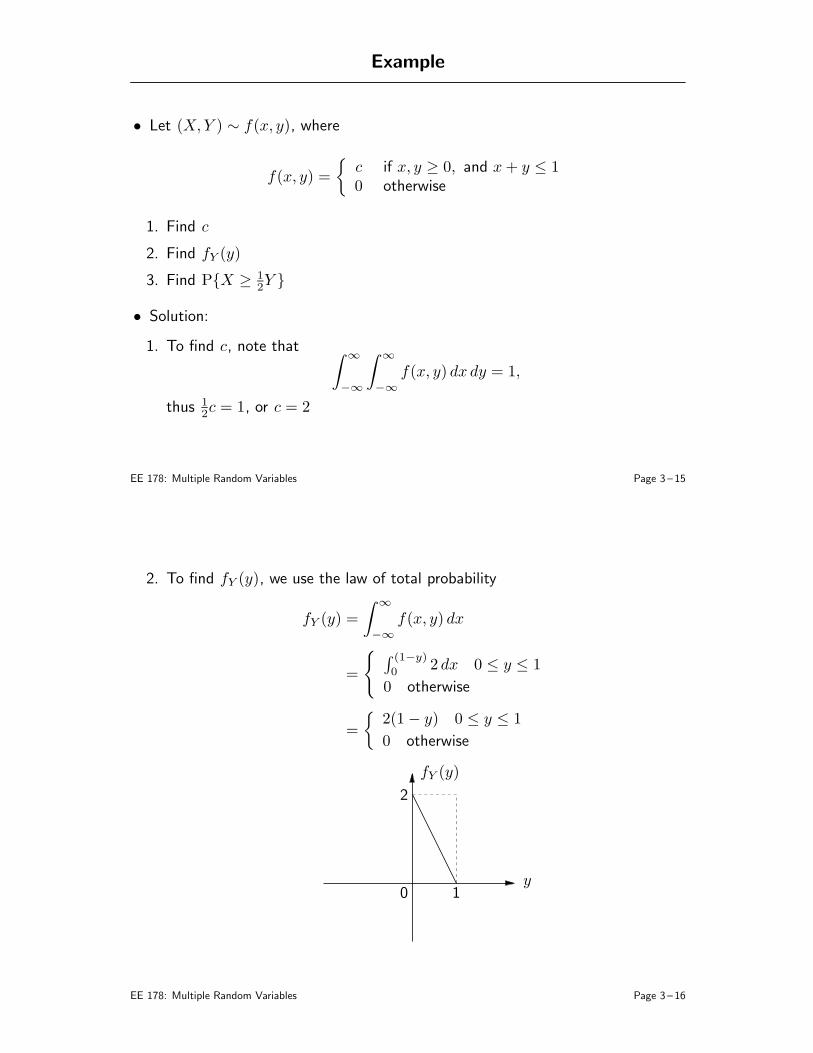
Example
• Let (X,Y ) ∼ f(x, y), where
f(x, y) =
c if x, y ≥ 0, and x+ y ≤ 10 otherwise
1. Find c
2. Find fY (y)
3. Find PX ≥ 12Y
• Solution:
1. To find c, note that∫
∞
−∞
∫
∞
−∞
f(x, y) dx dy = 1,
thus 12c = 1, or c = 2
EE 178: Multiple Random Variables Page 3 – 15
2. To find fY (y), we use the law of total probability
fY (y) =
∫
∞
−∞
f(x, y) dx
=
∫ (1−y)
02 dx 0 ≤ y ≤ 1
0 otherwise
=
2(1− y) 0 ≤ y ≤ 1
0 otherwise
y
fY (y)
2
0 1
EE 178: Multiple Random Variables Page 3 – 16
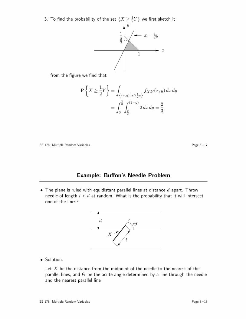
3. To find the probability of the set X ≥ 12Y we first sketch it
x
y
123
1
x = 12y
from the figure we find that
P
X ≥1
2Y
=
∫
(x,y):x≥12y
fX,Y (x, y) dx dy
=
∫ 23
0
∫ (1−y)
y2
2 dx dy =2
3
EE 178: Multiple Random Variables Page 3 – 17
Example: Buffon’s Needle Problem
• The plane is ruled with equidistant parallel lines at distance d apart. Throwneedle of length l < d at random. What is the probability that it will intersectone of the lines?
X
d
l
Θ
• Solution:
Let X be the distance from the midpoint of the needle to the nearest of theparallel lines, and Θ be the acute angle determined by a line through the needleand the nearest parallel line
EE 178: Multiple Random Variables Page 3 – 18
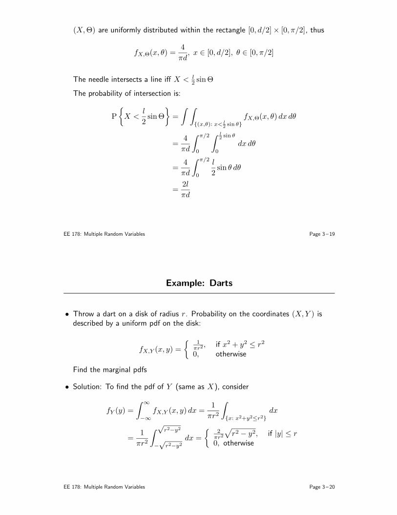
(X,Θ) are uniformly distributed within the rectangle [0, d/2]× [0, π/2], thus
fX,Θ(x, θ) =4
πd, x ∈ [0, d/2], θ ∈ [0, π/2]
The needle intersects a line iff X < l2 sinΘ
The probability of intersection is:
P
X <l
2sinΘ
=
∫ ∫
(x,θ): x< l2 sin θ
fX,Θ(x, θ) dx dθ
=4
πd
∫ π/2
0
∫ l2 sin θ
0
dx dθ
=4
πd
∫ π/2
0
l
2sin θ dθ
=2l
πd
EE 178: Multiple Random Variables Page 3 – 19
Example: Darts
• Throw a dart on a disk of radius r. Probability on the coordinates (X,Y ) isdescribed by a uniform pdf on the disk:
fX,Y (x, y) =
1πr2
, if x2 + y2 ≤ r2
0, otherwise
Find the marginal pdfs
• Solution: To find the pdf of Y (same as X), consider
fY (y) =
∫
∞
−∞
fX,Y (x, y) dx =1
πr2
∫
x: x2+y2≤r2
dx
=1
πr2
∫
√r2−y2
−
√r2−y2
dx =
2πr2
√
r2 − y2, if |y| ≤ r0, otherwise
EE 178: Multiple Random Variables Page 3 – 20
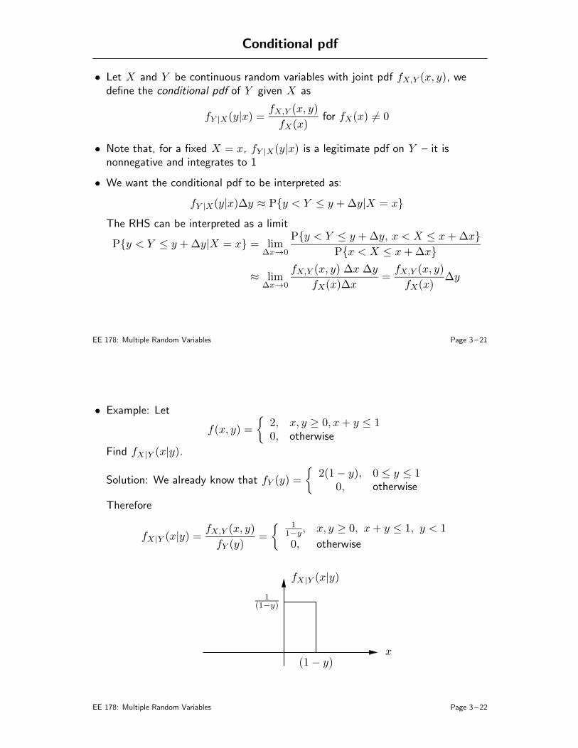
Conditional pdf
• Let X and Y be continuous random variables with joint pdf fX,Y (x, y), wedefine the conditional pdf of Y given X as
fY |X(y|x) =fX,Y (x, y)
fX(x)for fX(x) 6= 0
• Note that, for a fixed X = x, fY |X(y|x) is a legitimate pdf on Y – it isnonnegative and integrates to 1
• We want the conditional pdf to be interpreted as:
fY |X(y|x)∆y ≈ Py < Y ≤ y +∆y|X = x
The RHS can be interpreted as a limit
Py < Y ≤ y +∆y|X = x = lim∆x→0
Py < Y ≤ y +∆y, x < X ≤ x+∆x
Px < X ≤ x+∆x
≈ lim∆x→0
fX,Y (x, y) ∆x ∆y
fX(x)∆x=
fX,Y (x, y)
fX(x)∆y
EE 178: Multiple Random Variables Page 3 – 21
• Example: Let
f(x, y) =
2, x, y ≥ 0, x+ y ≤ 10, otherwise
Find fX|Y (x|y).
Solution: We already know that fY (y) =
2(1− y), 0 ≤ y ≤ 10, otherwise
Therefore
fX|Y (x|y) =fX,Y (x, y)
fY (y)=
11−y, x, y ≥ 0, x+ y ≤ 1, y < 1
0, otherwise
x
fX|Y (x|y)
1(1−y)
(1− y)
EE 178: Multiple Random Variables Page 3 – 22
• Chain rule: pX,Y (x, y) = pX(x)pY |X(y|x)
EE 178: Multiple Random Variables Page 3 – 23
Independence and Bayes Rule
• Independence: Two continuous r.v.s are said to be independent if
fX,Y (x, y) = fX(x)fY (y) for all x, y
It can be shown that this definition is equivalent to saying that X and Y areindependent if for any two events A,B ⊂ (−∞,∞)
PX ∈ A, Y ∈ B = PX ∈ APY ∈ B
• Example: Are X and Y in the previous example independent?
• Bayes rule for densities: Given fX(x) and fY |X(y|x), we can find
fX|Y (x|y) =fY |X(y|x)
fY (y)fX(x)
=fY |X(y|x)
∫
∞
−∞fX,Y (u, y)du
fX(x)
=fY |X(y|x)
∫
∞
−∞fX(u)fY |X(y|u) du
fX(x)
EE 178: Multiple Random Variables Page 3 – 24
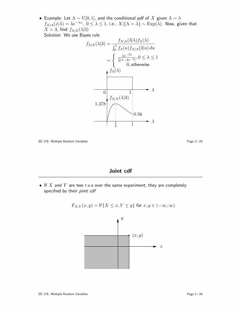
• Example: Let Λ ∼ U[0, 1], and the conditional pdf of X given Λ = λfX|Λ(x|λ) = λe−λx, 0 ≤ λ ≤ 1, i.e., X |Λ = λ ∼ Exp(λ). Now, given thatX = 3, find fΛ|X(λ|3)Solution: We use Bayes rule
fΛ|X(λ|3) =fX|Λ(3|λ)fΛ(λ)
∫ 1
0fΛ(u)fX|Λ(3|u) du
=
λe−3λ
19(1−4e−3)
, 0 ≤ λ ≤ 1
0, otherwise
λ
λ
fΛ(λ)
fΛ|X(λ|3)0
1
1
13
1.378
0.56
EE 178: Multiple Random Variables Page 3 – 25
Joint cdf
• If X and Y are two r.v.s over the same experiment, they are completelyspecified by their joint cdf
FX,Y (x, y) = PX ≤ x, Y ≤ y for x, y ∈ (−∞,∞)
x
y
(x, y)
EE 178: Multiple Random Variables Page 3 – 26
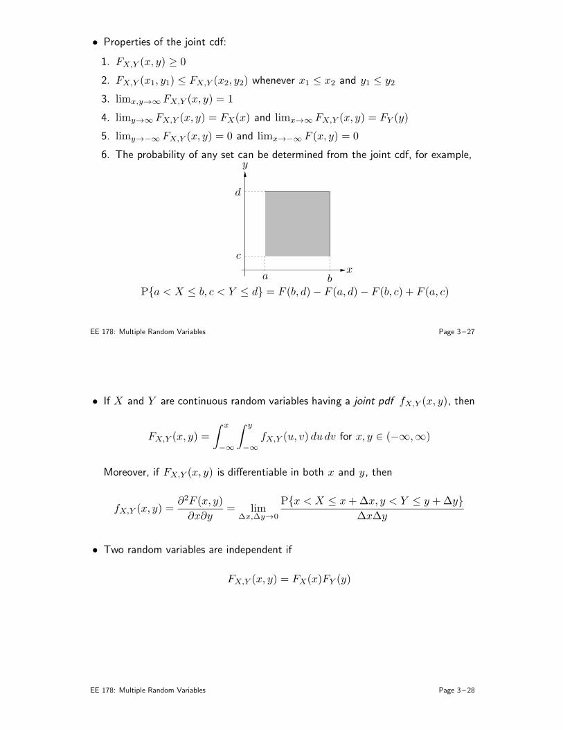
• Properties of the joint cdf:
1. FX,Y (x, y) ≥ 0
2. FX,Y (x1, y1) ≤ FX,Y (x2, y2) whenever x1 ≤ x2 and y1 ≤ y2
3. limx,y→∞FX,Y (x, y) = 1
4. limy→∞FX,Y (x, y) = FX(x) and limx→∞FX,Y (x, y) = FY (y)
5. limy→−∞ FX,Y (x, y) = 0 and limx→−∞ F (x, y) = 0
6. The probability of any set can be determined from the joint cdf, for example,
x
y
a b
c
d
Pa < X ≤ b, c < Y ≤ d = F (b, d)− F (a, d)− F (b, c) + F (a, c)
EE 178: Multiple Random Variables Page 3 – 27
• If X and Y are continuous random variables having a joint pdf fX,Y (x, y), then
FX,Y (x, y) =
∫ x
−∞
∫ y
−∞
fX,Y (u, v) dudv for x, y ∈ (−∞,∞)
Moreover, if FX,Y (x, y) is differentiable in both x and y, then
fX,Y (x, y) =∂2F (x, y)
∂x∂y= lim
∆x,∆y→0
Px < X ≤ x+∆x, y < Y ≤ y +∆y
∆x∆y
• Two random variables are independent if
FX,Y (x, y) = FX(x)FY (y)
EE 178: Multiple Random Variables Page 3 – 28
Functions of Two Random Variables
• Let X and Y be two r.v.s with known pdf fX,Y (x, y) and Z = g(x, y) be afunction of X and Y . We wish to find fZ(z)
• We use the same procedure as before: First calculate the cdf of Z , thendifferentiate it to find fZ(z)
• Example: Max and Min of Independent Random Variables
Let X ∼ fX(x) and Y ∼ fY (y) be independent, and define
U = maxX,Y , and V = minX,Y
Find the pdfs of U and V
• Solution: To find the pdf of U , we first find its cdf
FU(u) = PU ≤ u
= PX ≤ u, Y ≤ u
= FX(u)FY (u), by independence
EE 178: Multiple Random Variables Page 3 – 29
Now, to find the pdf, we take the derivative w.r.t. u
fU(u) = fX(u)FY (u) + fY (u)FX(u)
For example, if X and Y are uniformly distributed between 0 and 1,
fU(u) = 2u for 0 ≤ u ≤ 1
Next, to find the pdf of V , consider
FV (v) = PV ≤ v
= 1− PV > v
= 1− PX > v, Y > v
= 1− (1− FX(v))(1− FY (v))
= FX(v) + FY (v)− FX(v)FY (v),
thus
fV (v) = fX(v) + fY (v)− fX(v)FY (v)− fY (v)FX(v)
For example, if X ∼ Exp(λ1) and Y ∼ Exp(λ2), then V ∼ Exp(λ1 + λ2)
EE 178: Multiple Random Variables Page 3 – 30
Sum of Independent Random Variables
• Let X and Y be independent r.v.s with known distributions. We wish to findthe distribution of their sum W = X + Y
• First assume X ∼ pX(x) and Y ∼ pY (y) are independent integer-valued r.v.s,then for any integer w, the pmf of their sum
pW (w) = PX + Y = w
=∑
(x,y): x+y=w
PX = x, Y = y
=∑
x
PX = x, Y = w − x
=∑
x
PX = xPY = w − x, by independence
=∑
x
pX(x)pY (w − x)
This is the discrete convolution of the two pmfs
EE 178: Multiple Random Variables Page 3 – 31
For example, let X ∼ Poisson(λ1) and Y ∼ Poisson(λ2) be independent, thenthe pmf of their sum
pW (w) =
∞∑
x=−∞
pX(x)pY (w − x)
=w∑
x=0
pX(x)pY (w − x) for w = 0, 1, . . .
=
w∑
x=0
λx1
x!e−λ1
λw−x2
(w − x)!e−λ2
=(λ1 + λ2)
w
w!e−(λ1+λ2)
w∑
x=0
(
w
x
)(
λ1
λ1 + λ2
)x(λ2
λ1 + λ2
)w−x
=(λ1 + λ2)
w
w!e−(λ1+λ2)
Thus W = X + Y ∼ Poisson(λ1 + λ2)In general a Poisson r.v. with parameter λ can be written as the sum of anynumber of independent Poisson(λi) r.v.s, so long as
∑
λi = λ. This property ofa distribution is called infinite divisibility
EE 178: Multiple Random Variables Page 3 – 32
• Now, let’s assume that X ∼ fX(x), and Y ∼ fY (y) are independent continuousr.v.s. We wish to find the pdf of their sum W = X + Y . To do so, first notethat
PW ≤ w|X = x = PX + Y ≤ w|X = x
= Px+ Y ≤ w|X = x
= Px+ Y ≤ w, by independence
= FY (w − x)
ThusfW |X(w|x) = fY (w − x), a very useful result
Now, to find the pdf of W , consider
fW (w) =
∫
∞
−∞
fW,X(w, x) dx
=
∫
∞
−∞
fX(x)fW |X(w|x) dx =
∫
∞
−∞
fX(x)fY (w − x) dx
This is the convolution of fX(x) and fY (y)
EE 178: Multiple Random Variables Page 3 – 33
• Example: Assume that X ∼ U[0, 1] and Y ∼ U[0, 1] are independent r.v.s. Findthe pdf of their sum W = X + YSolution: To find the pdf of the sum, we convolve the two pdfs
fW (w) =
∫
∞
−∞
fX(x)fY (w − x) dx
=
∫ w
0dx, if 0 ≤ w ≤ 1
∫ 1
w−1dx, if 1 < w ≤ 2
0, otherwise
=
w, if 0 ≤ w ≤ 1
2− w, if 1 < w ≤ 2
0, otherwise
• Example: If X ∼ N (µ1, σ21) and Y ∼ N (µ2, σ
22) are indepedent, then their sum
W ∼ N (µ1 + µ2, σ21 + σ2
2), i.e., Gaussian is also an infinitely divisibledistribution– any Gaussian r.v. can be written as the sum of any number ofindependent Gaussians as long as their means sum to its mean and theirvariances sum to its variance (will prove this using transforms later)
EE 178: Multiple Random Variables Page 3 – 34
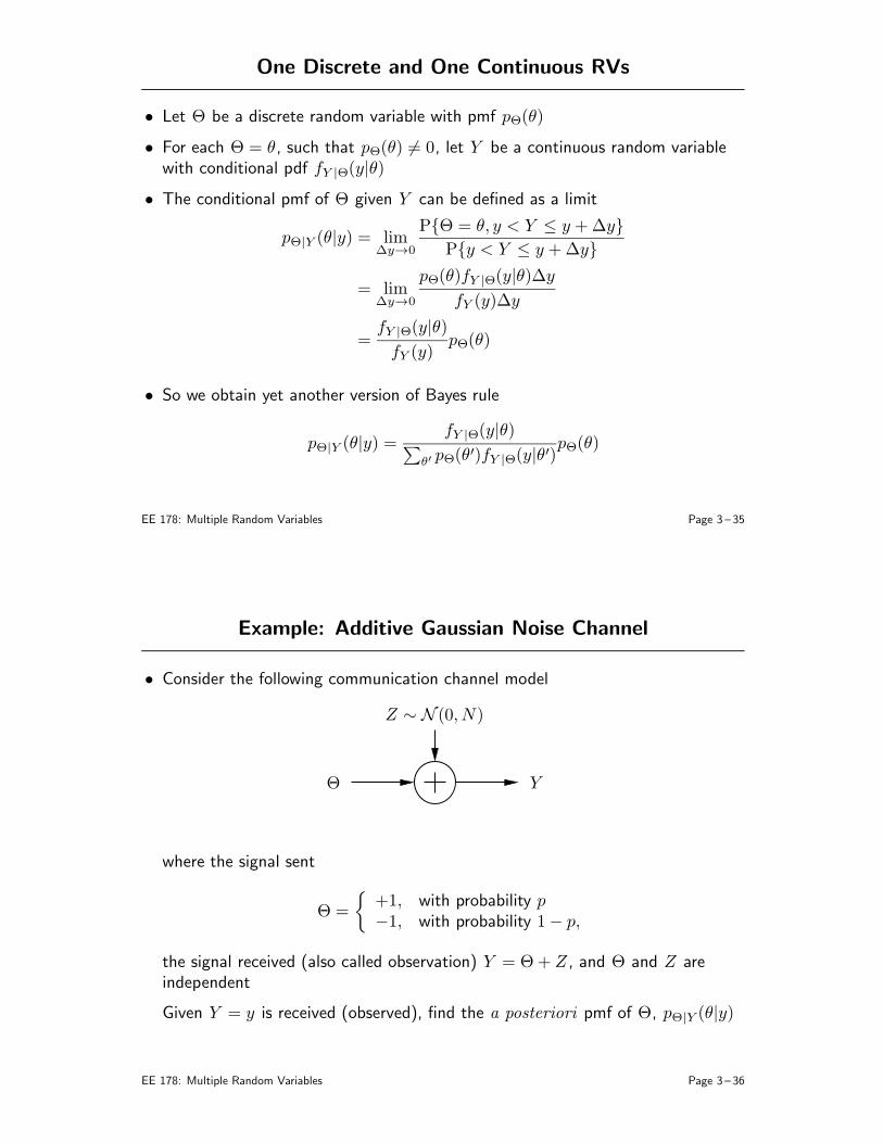
One Discrete and One Continuous RVs
• Let Θ be a discrete random variable with pmf pΘ(θ)
• For each Θ = θ, such that pΘ(θ) 6= 0, let Y be a continuous random variablewith conditional pdf fY |Θ(y|θ)
• The conditional pmf of Θ given Y can be defined as a limit
pΘ|Y (θ|y) = lim∆y→0
PΘ = θ, y < Y ≤ y +∆y
Py < Y ≤ y +∆y
= lim∆y→0
pΘ(θ)fY |Θ(y|θ)∆y
fY (y)∆y
=fY |Θ(y|θ)
fY (y)pΘ(θ)
• So we obtain yet another version of Bayes rule
pΘ|Y (θ|y) =fY |Θ(y|θ)
∑
θ′ pΘ(θ′)fY |Θ(y|θ′)
pΘ(θ)
EE 178: Multiple Random Variables Page 3 – 35
Example: Additive Gaussian Noise Channel
• Consider the following communication channel model
Θ Y
Z ∼ N (0, N)
where the signal sent
Θ =
+1, with probability p−1, with probability 1− p,
the signal received (also called observation) Y = Θ+ Z , and Θ and Z areindependent
Given Y = y is received (observed), find the a posteriori pmf of Θ, pΘ|Y (θ|y)
EE 178: Multiple Random Variables Page 3 – 36
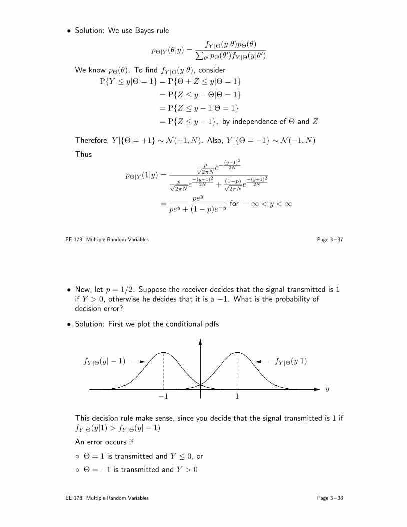
• Solution: We use Bayes rule
pΘ|Y (θ|y) =fY |Θ(y|θ)pΘ(θ)
∑
θ′ pΘ(θ′)fY |Θ(y|θ′)
We know pΘ(θ). To find fY |Θ(y|θ), consider
PY ≤ y|Θ = 1 = PΘ+ Z ≤ y|Θ = 1
= PZ ≤ y −Θ|Θ = 1
= PZ ≤ y − 1|Θ = 1
= PZ ≤ y − 1, by independence of Θ and Z
Therefore, Y |Θ = +1 ∼ N (+1, N). Also, Y |Θ = −1 ∼ N (−1, N)
Thus
pΘ|Y (1|y) =
p√
2πNe−
(y−1)2
2N
p√
2πNe−(y−1)2
2N + (1−p)√
2πNe−(y+1)2
2N
=pey
pey + (1− p)e−yfor −∞ < y < ∞
EE 178: Multiple Random Variables Page 3 – 37
• Now, let p = 1/2. Suppose the receiver decides that the signal transmitted is 1if Y > 0, otherwise he decides that it is a −1. What is the probability ofdecision error?
• Solution: First we plot the conditional pdfs
y
fY |Θ(y| − 1) fY |Θ(y|1)
1−1
This decision rule make sense, since you decide that the signal transmitted is 1 iffY |Θ(y|1) > fY |Θ(y| − 1)
An error occurs if
Θ = 1 is transmitted and Y ≤ 0, or
Θ = −1 is transmitted and Y > 0
EE 178: Multiple Random Variables Page 3 – 38
But if Θ = 1, then Y ≤ 0 iff Z < −1, and if Θ = −1, then Y > 0 iff Z > 1
Thus the probability of error is
P error = PΘ = 1, Y ≤ 0 or Θ = −1, Y > 0
= PΘ = 1, Y ≤ 0+ PΘ = −1, Y > 0
= PΘ = 1PY ≤ 0|Θ = 1+ PΘ = −1PY > 0|Θ = −1
=1
2PZ < −1+
1
2PZ > 1
= Q
(
1√N
)
EE 178: Multiple Random Variables Page 3 – 39
Summary: Total Probability and Bayes Rule
• Law of total probability:
events: P(B) =∑
iP(Ai ∩B), Ais partition Ω
pmf: pX(x) =∑
y p(x, y)
pdf: fX(x) =∫
fX,Y (x, y) dy
mixed: fY (y) =∑
θ pΘ(θ)fY |Θ(y|θ), pΘ(θ) =∫
fY (y)pΘ|Y (θ|y)dy
• Bayes rule:
events: P(Aj|B) =P(B|Aj)
∑
i P(B|Ai)P(Ai)P(Aj), Ais partition Ω
pmf: pX|Y (x|y) =pY |X(y|x)
∑
x′ pY |X(y|x′)pX(x′)pX(x)
pdf: fX|Y (x|y) =fY |X(y|x)
∫
fX(x′)fY |X(y|x′) dx′fX(x)
mixed: pΘ|Y (θ|y) =fY |Θ(y|θ)
∑
θ′ pΘ(θ′)fY |Θ(y|θ′) pΘ(θ),
fY |Θ(y|θ) =pΘ|Y (θ|y)
∫
fY (y′)pΘ|Y (θ|y′)dy′fY (y)
EE 178: Multiple Random Variables Page 3 – 40
More Than Two RVs
• Let X1, X2, . . . , Xn be random variables (defined over the same experiment)
• If the r.v.s are discrete then they can be jointly specified by their joint pmf
pX1,X2,...,Xn(x1, x2, . . . , xn), for all (x1, x2, . . . , xn) ∈ X1 ×X2×, . . .×Xn
• If the r.v.s are jointly continuous, then they can be specified by the joint pdf
fX1,X2,...,Xn(x1, x2, . . . , xn), for all (x1, x2, . . . , xn)
• Marginal pdf (or pmf) is the joint pdf (or pmf) for a subset of X1, . . . , Xn;e.g. for three r.v.s X1, X2, X3, the marginals are fXi(xi) and fXi,Xj(xi, xj) fori 6= j
• The marginals can be obtained from the joint in the usual way, e.g. for then = 3 example
fX1,X2(x1, x2) =
∫
∞
−∞
fX1,X2,X3(x1, x2, x3) dx3
EE 178: Multiple Random Variables Page 3 – 41
• Conditional pmf or pdf can be defined in the usual way, e.g. the conditional pdfof (Xk+1, Xk+2, . . . ,Xn) given (X1, X2, . . . , Xk) is
fXk+1,...,Xn|X1,...,Xk(xk+1, . . . , xn|x1, . . . , xk) =
fX1,...,Xn(x1, . . . , xn)
fX1,...,Xk(x1, . . . , xk)
• Chain rule: We can write
fX1,...,Xn(x1, . . . , xn) = fX1(x1)fX2|X1(x2|x1)fX3|X1,X2
(x3|x1, x2) . . .
. . . fXn|X1,...,Xn−1(xn|x1, . . . , xn−1)
• In general X1, X2, . . . , Xn are completely specified by their joint cdf
FX1,...,Xn(x1, . . . , xn) = PX1 ≤ x1, . . . ,Xn ≤ xn, for all (x1, . . . , xn)
EE 178: Multiple Random Variables Page 3 – 42
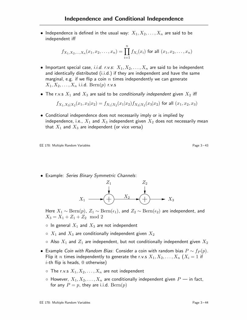
Independence and Conditional Independence
• Independence is defined in the usual way: X1,X2, . . . ,Xn are said to beindependent iff
fX1,X2,...,Xn(x1, x2, . . . , xn) =n∏
i=1
fXi(xi) for all (x1, x2, . . . , xn)
• Important special case, i.i.d. r.v.s: X1,X2, . . . ,Xn are said to be independentand identically distributed (i.i.d.) if they are independent and have the samemarginal, e.g. if we flip a coin n times independently we can generateX1,X2, . . . ,Xn i.i.d. Bern(p) r.v.s
• The r.v.s X1 and X3 are said to be conditionally independent given X2 iff
fX1,X3|X2(x1, x3|x2) = fX1|X2
(x1|x2)fX3|X2(x3|x2) for all (x1, x2, x3)
• Conditional independence does not necessarily imply or is implied byindependence, i.e., X1 and X3 independent given X2 does not necessarily meanthat X1 and X3 are independent (or vice versa)
EE 178: Multiple Random Variables Page 3 – 43
• Example: Series Binary Symmetric Channels:
X1X2 X3
Z1 Z2
Here X1 ∼ Bern(p), Z1 ∼ Bern(ǫ1), and Z2 ∼ Bern(ǫ2) are independent, andX3 = X1 + Z1 + Z2 mod 2
In general X1 and X3 are not independent
X1 and X3 are conditionally independent given X2
Also X1 and Z1 are independent, but not conditionally independent given X2
• Example Coin with Random Bias: Consider a coin with random bias P ∼ fP (p).Flip it n times independently to generate the r.v.s X1,X2, . . . ,Xn (Xi = 1 ifi-th flip is heads, 0 otherwise)
The r.v.s X1,X2, . . . ,Xn are not independent
However, X1, X2, . . . , Xn are conditionally independent given P — in fact,for any P = p, they are i.i.d. Bern(p)
EE 178: Multiple Random Variables Page 3 – 44
Lecture Notes 4
Expectation
• Definition and Properties
• Covariance and Correlation
• Linear MSE Estimation
• Sum of RVs
• Conditional Expectation
• Iterated Expectation
• Nonlinear MSE Estimation
• Sum of Random Number of RVs
Corresponding pages from B&T: 81-92, 94-98, 104-115, 160-163, 171-174, 179, 225-233, 236-247.
EE 178: Expectation Page 4 – 1
Definition
• We already introduced the notion of expectation (mean) of a r.v.
• We generalize this definition and discuss it in more depth
• Let X ∈ X be a discrete r.v. with pmf pX(x) and g(x) be a function of x. Theexpectation or expected value of g(X) is defined as
E(g(X)) =∑
x∈X
g(x)pX(x)
• For a continuous r.v. X ∼ fX(x), the expected value of g(X) is defined as
E(g(X)) =
∫
∞
−∞
g(x)fX(x) dx
• Examples:
g(X) = c, a constant, then E(g(X)) = c
g(X) = X , E(X) =∑
x xpX(x) is the mean of X
g(X) = Xk, E(Xk) is the kth moment of X
g(X) = (X − E(X))2, E[
(X − E(X))2]
is the variance of X
EE 178: Expectation Page 4 – 2
• Expectation is linear, i.e., for any constants a and b
E [ag1(X) + bg2(X)] = aE(g1(X)) + bE(g2(X))
Examples:
E(aX + b) = aE(X) + b
Var(aX + b) = a2Var(X)Proof: From the definition
Var(aX + b) = E[
((aX + b)− E(aX + b))2]
= E[
(aX + b− aE(X)− b)2]
= E[
a2(X − E(X))2]
= a2E(
(X − E(X))2)
= a2Var(X)
EE 178: Expectation Page 4 – 3
Fundamental Theorem of Expectation
• Theorem: Let X ∼ pX(x) and Y = g(X) ∼ pY (y), then
E(Y ) =∑
y∈Y
ypY (y) =∑
x∈X
g(x)pX(x) = E(g(X))
• The same formula holds for fY (y) using integrals instead of sums
• Conclusion: E(Y ) can be found using either fX(x) or fY (y). It is often mucheasier to use fX(x) than to first find fY (y) then find E(Y )
• Proof: We prove the theorem for discrete r.v.s. Consider
E(Y ) =∑
y
ypY (y)
=∑
y
y∑
x: g(x)=y
pX(x)
=∑
y
∑
x: g(x)=y
ypX(x)
=∑
y
∑
x: g(x)=y
g(x)pX(x) =∑
x
g(x)pX(x)
EE 178: Expectation Page 4 – 4
Expectation Involving Two RVs
• Let (X,Y ) ∼ fX,Y (x, y) and let g(x, y) be a function of x and y. Theexpectation of g(X,Y ) is defined as
E(g(X,Y )) =
∫
∞
−∞
∫
∞
−∞
g(x, y)fX,Y (x, y) dx dy
The function g(X, Y ) may be X , Y , X2, X + Y , etc.
• The correlation of X and Y is defined as E(XY )
• The covariance of X and Y is defined as
Cov(X,Y ) = E [(X − E(X))(Y − E(Y ))]
= E [XY −X E(Y )− Y E(X) + E(X) E(Y )]
= E(XY )− E(X) E(Y )
Note that if X = Y , then Cov(X,Y ) = Var(X)
EE 178: Expectation Page 4 – 5
• Example: Let
f(x, y) =
2 for x, y ≥ 0, x+ y ≤ 10 otherwise
Find E(X), Var(X), and Cov(X,Y )
Solution: The mean is
E(X) =
∫
∞
−∞
∫
∞
−∞
xf(x, y) dy dx
=
∫ 1
0
∫ 1−x
0
2x dy dx = 2
∫ 1
0
(1− x)x dx =1
3
To find the variance, we first find the second moment
E(X2) =
∫ 1
0
∫ 1−x
0
2x2 dy dx = 2
∫ 1
0
(1− x)x2 dx =1
6
Thus,
Var(X) = E(X2)− (E(X))2 =1
6−
1
9=
1
18
EE 178: Expectation Page 4 – 6
The covariance of X and Y is
Cov(X,Y ) = 2
∫ 1
0
∫ 1−x
0
xy dy dx− E(X)E(Y )
=
∫ 1
0
x(1− x)2 dx−1
9=
1
12−
1
9= −
1
36
EE 178: Expectation Page 4 – 7
Independence and Uncorrelation
• Let X and Y be independent r.v.s and g(X) and h(Y ) be functions of X andY , respectively, then
E(g(X)h(Y )) = E(g(X)) E(h(Y ))
Proof: Let’s assume that X ∼ fX(x) and Y ∼ fY (y), then
E(g(X)h(Y )) =
∫
∞
−∞
∫
∞
−∞
g(x)h(y)fX,Y (x, y) dx dy
=
∫
∞
−∞
∫
∞
−∞
g(x)h(y)fX(x)fY (y) dx dy
=
∫
∞
−∞
g(x)fX(x) dx
∫
∞
−∞
h(y)fY (y) dy
= E(g(X)) E(h(Y ))
• X and Y are said to be uncorrelated if Cov(X, Y ) = 0, or equivalentlyE(XY ) = E(X) E(Y )
EE 178: Expectation Page 4 – 8
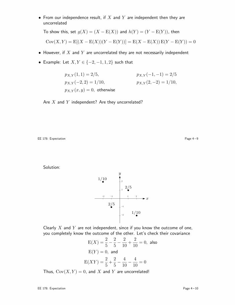
• From our independence result, if X and Y are independent then they areuncorrelated
To show this, set g(X) = (X − E(X)) and h(Y ) = (Y − E(Y )), then
Cov(X, Y ) = E[(X − E(X))(Y − E(Y ))] = E(X − E(X)) E(Y − E(Y )) = 0
• However, if X and Y are uncorrelated they are not necessarily independent
• Example: Let X, Y ∈ −2,−1, 1, 2 such that
pX,Y (1, 1) = 2/5, pX,Y (−1,−1) = 2/5
pX,Y (−2, 2) = 1/10, pX,Y (2,−2) = 1/10,
pX,Y (x, y) = 0, otherwise
Are X and Y independent? Are they uncorrelated?
EE 178: Expectation Page 4 – 9
Solution:
1
2
−2 −1 2
−1
−2
1x
y
1/10
1/10
2/5
2/5
Clearly X and Y are not independent, since if you know the outcome of one,you completely know the outcome of the other. Let’s check their covariance
E(X) =2
5−
2
5−
2
10+
2
10= 0, also
E(Y ) = 0, and
E(XY ) =2
5+
2
5−
4
10−
4
10= 0
Thus, Cov(X,Y ) = 0, and X and Y are uncorrelated!
EE 178: Expectation Page 4 – 10
The Correlation Coefficient
• The correlation coefficient of X and Y is defined as
ρX,Y =Cov(X,Y )
√
Var(X)Var(Y )
• Fact: |ρX,Y | ≤ 1. To show this consider
E
[
(
X − E(X)
σX
±Y − E(Y )
σY
)2]
≥ 0
E[
(X − E(X))2]
σ2X
+E[
(Y − E(Y ))2]
σ2Y
± 2E[
(X − E(X))(Y − E(Y ))]
σXσY
≥ 0
1 + 1± 2ρX,Y ≥ 0 =⇒ −2 ≤ 2ρX,Y ≤ 2 =⇒ |ρX,Y | ≤ 1
• From the proof, ρX,Y = ±1 iff (X − E(X))/σX = ±(Y − E(Y ))/σY (equalitywith probability 1), i.e., iff X − E(X) is a linear function of Y − E(Y )
• In general ρX,Y is a measure of how closely (X − E(X)) can be approximatedor estimated by a linear function of (Y − E(Y ))
EE 178: Expectation Page 4 – 11
Application: Linear MSE Estimation
• Consider the following signal processing problem:
X XY
aX + b
NoisyChannel Estimator
• Here X is a signal (music, speech, image) and Y is a noisy observation of X(output of a noisy communication channel or a noisy circuit). Assume we knowthe means, variances and covariance of X and Y
• Observing Y , we wish to find a linear estimate of X of the form X = aY + b,which minimizes the mean square error
MSE = E[
(X − X)2]
• We denote the best such estimate as the minimum mean square estimate(MMSE)
EE 178: Expectation Page 4 – 12
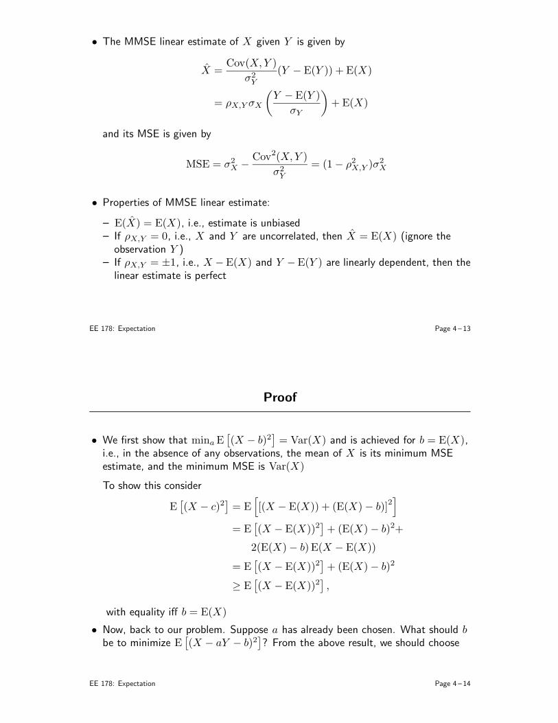
• The MMSE linear estimate of X given Y is given by
X =Cov(X,Y )
σ2Y
(Y − E(Y )) + E(X)
= ρX,Y σX
(
Y − E(Y )
σY
)
+ E(X)
and its MSE is given by
MSE = σ2X −
Cov2(X,Y )
σ2Y
= (1− ρ2X,Y )σ2X
• Properties of MMSE linear estimate:
– E(X) = E(X), i.e., estimate is unbiased– If ρX,Y = 0, i.e., X and Y are uncorrelated, then X = E(X) (ignore the
observation Y )– If ρX,Y = ±1, i.e., X −E(X) and Y −E(Y ) are linearly dependent, then the
linear estimate is perfect
EE 178: Expectation Page 4 – 13
Proof
• We first show that minaE[
(X − b)2]
= Var(X) and is achieved for b = E(X),i.e., in the absence of any observations, the mean of X is its minimum MSEestimate, and the minimum MSE is Var(X)
To show this consider
E[
(X − c)2]
= E[
[(X − E(X)) + (E(X)− b)]2]
= E[
(X − E(X))2]
+ (E(X)− b)2+
2(E(X)− b) E(X − E(X))
= E[
(X − E(X))2]
+ (E(X)− b)2
≥ E[
(X − E(X))2]
,
with equality iff b = E(X)
• Now, back to our problem. Suppose a has already been chosen. What should bbe to minimize E
[
(X − aY − b)2]
? From the above result, we should choose
EE 178: Expectation Page 4 – 14
b = E(X − aY ) = E(X)− aE(Y )
So, we want to choose a to minimize
E[
((X − aY )− E(X − aY ))2]
,
which is the same as
E[
((X − E(X))− a(Y − E(Y )))2]
= σ2X + a2σ2
Y − 2aCov(X,Y )
This is a quadratic function of a. It is minimized when its derivative equals 0,which gives
a =Cov(X,Y )
σ2Y
=ρX,Y σXσY
σ2Y
=ρX,Y σX
σY
The mean square error is given by
σ2X + a2σ2
Y − 2aCov(X,Y ) = σ2X +
ρ2X,Y σ2X
σ2Y
σ2Y − 2
ρX,Y σX
σY× ρX,Y σXσY
= (1− ρ2X,Y )σ2X
EE 178: Expectation Page 4 – 15
Mean and Variance of Sum of RVs
• Let X1,X2, . . . ,Xn be r.v.s, then by linearity of expectation, the expected valueof their sum Y is
E(Y ) = E
(
n∑
i=1
Xi
)
=
n∑
i=1
E(Xi)
Example: Mean of Binomial r.v. One way to define a binomial r.v. is as follows:Flip a coin with bias p independently n times and define the Bernoulli r.v.Xi = 1 if the ith flip is a head and 0 if it is a tail. Let Y =
∑ni=1Xi. Then Y
is a binomial r.v.
Thus
E(Y ) =n∑
i=1
E(Xi) = np
Note that we do not need independence for this result to hold, i.e., the resultholds even if the coin flips are not independent (Y is not binomial in this case,but the expectation doesn’t change)
EE 178: Expectation Page 4 – 16
• Let’s compute the variance of Y =∑n
i=1Xi
Var(Y ) = E[
(Y − E(Y ))2]
= E
(
n∑
i=1
Xi −
n∑
i=1
E(Xi)
)2
= E
(
n∑
i=1
(Xi − E(Xi))
)2
= E
n∑
i=1
n∑
j=1
(Xi − E(Xi))(Xj − E(Xj))
=n∑
i=1
n∑
j=1
E[(Xi − E(Xi))(Xj − E(Xj))]
=n∑
i=1
Var(Xi) +n∑
i=1
n∑
j 6=i
Cov(Xi,Xj)
EE 178: Expectation Page 4 – 17
• If the r.v.s are independent, then Cov(Xi, Xj) = 0 for all i 6= j , and
Var(Y ) =
n∑
i=1
Var(Xi)
Note that this result only requires that Cov(Xi,Xj) = 0, for all i 6= j , andtherefore it requires that the r.v.s be uncorrelated (which is in general weakerthan independence)
• Example: Variance of Binomial r.v. Again express Y =∑n
i=1Xi, where the Xisare i.i.d. Bern(p). Since the Xis are independent, Cov(Xi, Xj) = 0, for alli 6= j . Thus
Var(Y ) =n∑
i=1
Var(Xi) = n× p(1− p)
• Example: Hat problem Suppose n people throw their hats in a box and theneach picks one hat at random. Let N be the number of people that get backtheir own hat. Find E(N) and Var(N)
Solution: Define the r.v. Xi = 1 if a person selects her own hat, and Xi = 0,otherwise. Thus N =
∑ni=1Xi
EE 178: Expectation Page 4 – 18
To find the mean and variance of N , we first find the means, variances andcovariances of the Xis. Note that Xi ∼ Bern(1/n) and thus E(Xi) = 1/n, andVar(Xi) = (1/n)(1− 1/n). To find the covariance of Xi and Xj , i 6= j , notethat
pXi,Xj(1, 1) =
1
n(n− 1)Thus,
Cov(Xi,Xj) = E(XiXj)− E(Xi) E(Xj) =1
n(n− 1)× 1−
(
1
n
)2
=1
n2(n− 1)
The mean and variance of N are given by
E(N) = nE(X1) = 1
Var(N) =n∑
i=1
Var(Xi) +n∑
i=1
n∑
j 6=i
Cov(Xi, Xj)
= n×Var(X1) + n(n− 1)Cov(X1,X2)
= (1− 1/n) + n(n− 1)×1
n2(n− 1)= 1
EE 178: Expectation Page 4 – 19
Method of Indicators
• In the last two examples we used the method of indicators to simplify thecomputation of expectation
• In general the indicator of an event A ⊂ Ω is a r.v. defined as
IA(ω) =
1 if x ∈ A0 otherwise
ThusE(IA) = 1× P(A) + 0× P(Ac) = P(A)
The method of indicators involves expressing a given r.v. Y as a sum ofindicators in order to simplify the computation of its expectation (this isprecisely what we did in the last two examples)
Example: Spaghetti. Consider a ball of n spaghetti strands. You randomly picktwo strand ends and join them. The process is continued until there are no endsleft. Let X be the number of spaghetti loops formed. What is E(X)?
EE 178: Expectation Page 4 – 20
Conditional Expectation
• Conditioning on an event: Let X ∼ pX(x) be a r.v. and A be a nonzeroprobability event. We can define the conditional pmf of X given X ∈ A as
pX|A(x) = PX = x|X ∈ A =PX = x,X ∈ A
PX ∈ A=
pX(x)PX∈A
, if x ∈ A
0, otherwise
Note that pX|A(x) is a pmf on X
• Similarly for X ∼ fX(x),
fX|A(x) =
fX(x)PX∈A
, if x ∈ A
0, otherwise
is a pdf on X
• Example: Let X ∼ Exp(λ) and A = X > a, for some constant a > 0. Findthe conditional pdf of X given A
EE 178: Expectation Page 4 – 21
• We define the conditional expectation of g(X) given X ∈ A as
E(g(X)|A) =
∫
∞
−∞
g(x)fX|A(x) dx
• Example: Find E(X |A) and E(X2|A) for the previous example.
• Total expectation: Let X ∼ fX(x) and A1, A2, . . . , An ⊂ (−∞,∞) be disjointnonzero probability events with PX ∈ ∪n
i=1Ai =∑n
i=1PX ∈ Ai = 1, then
E(g(X)) =n∑
i=1
PX ∈ AiE(g(X)|Ai)
This is called the total expectation theorem and is useful in computingexpectation by divide-and-conquer
Proof: First note that by the law of total probability
fX(x) =n∑
i=1
PX ∈ AifX|Ai(x)
EE 178: Expectation Page 4 – 22
Therefore
E(g(X)) =
∫
∞
−∞
g(x)fX(x) dx
=
∫
∞
−∞
g(x)
n∑
i=1
PX ∈ AifX|Ai(x) dx
=
n∑
i=1
PX ∈ Ai
∫
∞
−∞
g(x)fX|Ai(x) dx =
n∑
i=1
PX ∈ AiE(g(X)|Ai)
• Example: mean and variance of Piecewise uniform pdf Let X be a continuousr.v. with the piecewise uniform pdf
fX(x) =
1/3, if 0 ≤ x ≤ 12/3, if 1 < x ≤ 20, otherwise
Find the mean and variance of X
EE 178: Expectation Page 4 – 23
Solution: Define the events A1 = X ∈ [0, 1] and A2 = X ∈ (1, 2]
Then, A1, A2 are disjoint and the sum of their probabilities is 1. The mean ofX can be expressed as
E(X) =
2∑
i=1
PX ∈ AiE(X |Ai) =1
3×
1
2+
2
3×
3
2=
7
6
Also
E(X2) =2∑
i=1
PX ∈ AiE(X2|Ai) =
1
3×
1
3+
2
3×
7
3=
15
9Thus
Var(X) = E(X2)− (E(X))2 =11
36
• Mean and variance of a mixed r.v. As we discussed, there are r.v.s that areneither discrete nor continuous. How do we define their expectation?
EE 178: Expectation Page 4 – 24
Answer: We can express a mixed r.v. X as a mixture of a discrete r.v. Y and acontinuous r.v. Z as follows
Assume that the cdf of X is discontinuous over the set Y and that∑
y∈YPX = y = p. Define the discrete r.v. Y ∈ Y to have the pmf
pY (y) =1
pPX = y, y ∈ Y
Define the continuous r.v. Z such that
fZ(z) =
11−p
dFXdx z /∈ Y
fZ(z−) z ∈ Y
Now, we can express X as
X =
Y with probability pZ with probability 1− p
To find E(X), we use the law of total expectation
E(X) = pE(X |X ∈ Y) + (1− p) E(X |X /∈ Y) = pE(Y ) + (1− p) E(Z)
Now both E(Y ) and E(Z) can be computed in the usual way
EE 178: Expectation Page 4 – 25
Conditioning on a RV
• Let (X,Y ) ∼ fX,Y (x, y). If fY (y) 6= 0, the conditional pdf of X given Y = yis given by
fX|Y (x|y) =fX,Y (x, y)
fY (y)
• We know that fX|Y (x|y) is a pdf for X (function of y), so we can define theexpectation of any function g(X, Y ) w.r.t. fX|Y (x|y) as
E(g(X,Y )|Y = y) =
∫
∞
−∞
g(x, y)fX|Y (x|y) dx
• If g(X, Y ) = X , then, the conditional expectation of X given Y = y is
E(X |Y = y) =
∫
∞
−∞
xfX|Y (x|y) dx
EE 178: Expectation Page 4 – 26
• Example: Let
fX,Y (x, y) =
2 for x, y ≥ 0, x+ y ≤ 10 otherwise
Find E(X |Y = y) and E(XY |Y = y)
Solution: We already know that
fX|Y (x|y) =
11−y for x, y ≥ 0, x+ y ≤ 1, y < 1
0 otherwise ,
thus
E(X |Y = y) =
∫ 1−y
0
1
1− yx dx
=1− y
2for 0 ≤ y < 1
Now to find E(XY |Y = y), note that
E(XY |Y = y) = yE(X |Y = y)
=y(1− y)
2for 0 ≤ y < 1
EE 178: Expectation Page 4 – 27
Conditional Expectation as a RV
• We define the conditional expectation of g(X,Y ) given Y as the randomvariable E(g(X,Y )|Y ), which is a function of the random variable Y
• So, E(X |Y ) is the conditional expectation of X given Y , a r.v. that is afunction of Y
• Example: This is a continuation of the previous example. Find the pdf ofE(X |Y )
Solution: The conditional expectation of X given Y is the r.v.
E(X |Y ) =1− Y
2
= Z
The pdf of Z is given by
fZ(z) = 8z for 0 < z ≤1
2
EE 178: Expectation Page 4 – 28
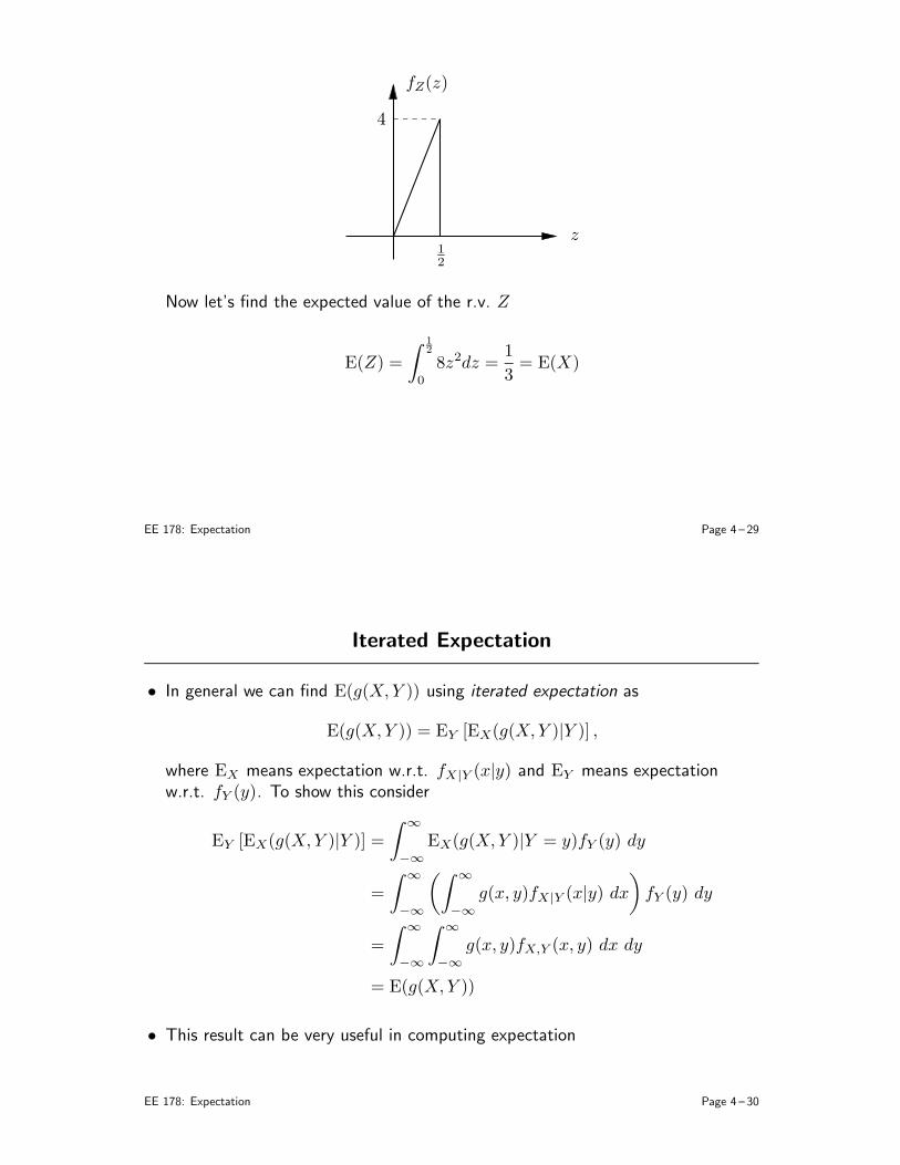
fZ(z)
z
4
12
Now let’s find the expected value of the r.v. Z
E(Z) =
∫ 12
0
8z2dz =1
3= E(X)
EE 178: Expectation Page 4 – 29
Iterated Expectation
• In general we can find E(g(X,Y )) using iterated expectation as
E(g(X,Y )) = EY [EX(g(X,Y )|Y )] ,
where EX means expectation w.r.t. fX|Y (x|y) and EY means expectationw.r.t. fY (y). To show this consider
EY [EX(g(X,Y )|Y )] =
∫
∞
−∞
EX(g(X,Y )|Y = y)fY (y) dy
=
∫
∞
−∞
(∫
∞
−∞
g(x, y)fX|Y (x|y) dx
)
fY (y) dy
=
∫
∞
−∞
∫
∞
−∞
g(x, y)fX,Y (x, y) dx dy
= E(g(X,Y ))
• This result can be very useful in computing expectation
EE 178: Expectation Page 4 – 30
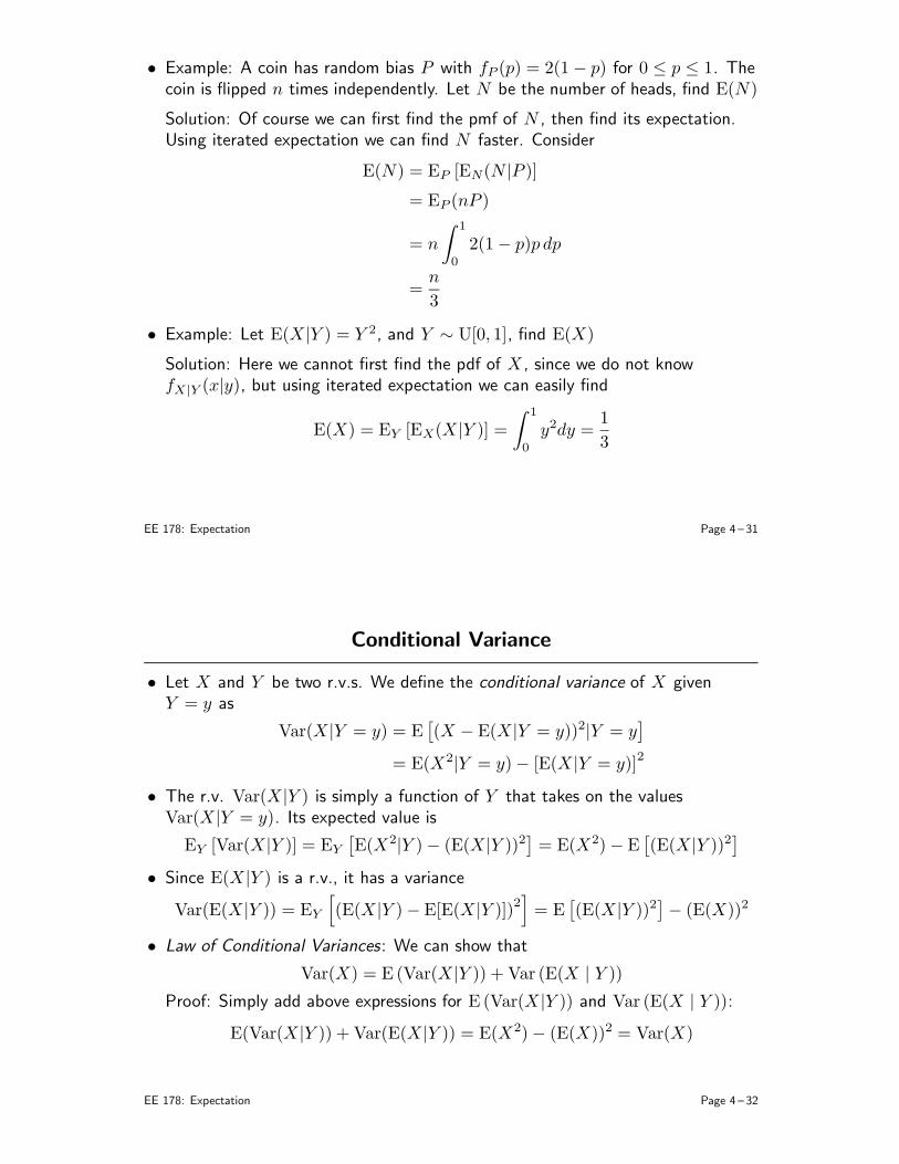
• Example: A coin has random bias P with fP (p) = 2(1− p) for 0 ≤ p ≤ 1. Thecoin is flipped n times independently. Let N be the number of heads, find E(N)
Solution: Of course we can first find the pmf of N , then find its expectation.Using iterated expectation we can find N faster. Consider
E(N) = EP [EN(N |P )]
= EP (nP )
= n
∫ 1
0
2(1− p)p dp
=n
3
• Example: Let E(X |Y ) = Y 2, and Y ∼ U[0, 1], find E(X)
Solution: Here we cannot first find the pdf of X , since we do not knowfX|Y (x|y), but using iterated expectation we can easily find
E(X) = EY [EX(X |Y )] =
∫ 1
0
y2dy =1
3
EE 178: Expectation Page 4 – 31
Conditional Variance
• Let X and Y be two r.v.s. We define the conditional variance of X givenY = y as
Var(X |Y = y) = E[
(X − E(X |Y = y))2|Y = y]
= E(X2|Y = y)− [E(X |Y = y)]2
• The r.v. Var(X |Y ) is simply a function of Y that takes on the valuesVar(X |Y = y). Its expected value is
EY [Var(X |Y )] = EY
[
E(X2|Y )− (E(X |Y ))2]
= E(X2)− E[
(E(X |Y ))2]
• Since E(X |Y ) is a r.v., it has a variance
Var(E(X |Y )) = EY
[
(E(X |Y )− E[E(X |Y )])2]
= E[
(E(X |Y ))2]
− (E(X))2
• Law of Conditional Variances: We can show that
Var(X) = E (Var(X |Y )) + Var (E(X | Y ))
Proof: Simply add above expressions for E (Var(X |Y )) and Var (E(X | Y )):
E(Var(X |Y )) + Var(E(X |Y )) = E(X2)− (E(X))2 = Var(X)
EE 178: Expectation Page 4 – 32
Application: Nonlinear MSE Estimation
• Consider the estimation setup with signal X, observation Y
• Assume we know the pdf of X and the conditional pdf of the channelfY |X(y|x) for all (x, y)
• We wish to find the best nonlinear estimate X = g(Y ) of X that minimizes themean square error
MSE = E[
(X − X)2]
= E[
(X − g(Y ))2]
• The X that achieves the minimum MSE is called the minimum MSE estimate(MMSE) of X (given Y )
EE 178: Expectation Page 4 – 33
MMSE Estimate
• The MMSE estimate of X given the observation Y and complete knowledge ofthe joint pdf fX,Y (x, y) is
X = E(X |Y )
and its MSE (i.e., minimum MSE) is
MSE = E[
(X − E(X |Y ))2]
= E[
E[
(X − E(X |Y ))2∣
∣Y]]
= EY [Var(X |Y )]
• Proof:
Recall that minaE[
(X − a)2]
= Var(X) and is achieved for a = E(X), i.e.,in the absence of any observations, the mean of X is its minimum MSEestimate, and the minimum MSE is Var(X)
We now use this result to show that E(X |Y ) is the MMSE estimate of Xgiven Y . First we use iterated expectation to write
EE 178: Expectation Page 4 – 34
E[
(X − g(Y ))2]
= EY
[
EX
[
(X − g(Y ))2|Y]]
From the above result we know that for each Y = y,EX
[
(X − g(y))2|Y = y]
is minimum for g(y) = E(X |Y = y). Thus theMSE is minimized for g(Y ) = E(X |Y )Thus E(X |Y ) minimizes the MSE conditioned on every Y = y and not justits average over Y !
EE 178: Expectation Page 4 – 35
• Properties of the minimum MSE estimator:
Since E(X) = E[E(X |Y )] = E(X), the best MSE estimate is called unbiased
If X and Y are independent, then the best MSE estimate is E(X)
The conditional expectation of the estimation error E((X − X)|Y = y) = 0for all y, i.e., the error is unbiased for every Y = y
From the law of conditional variance
Var(X) = Var(X) + E(Var(X |Y )),
i.e., the sum of the variance of the estimate and the minimum MSE is equalto the variance of the signal
EE 178: Expectation Page 4 – 36
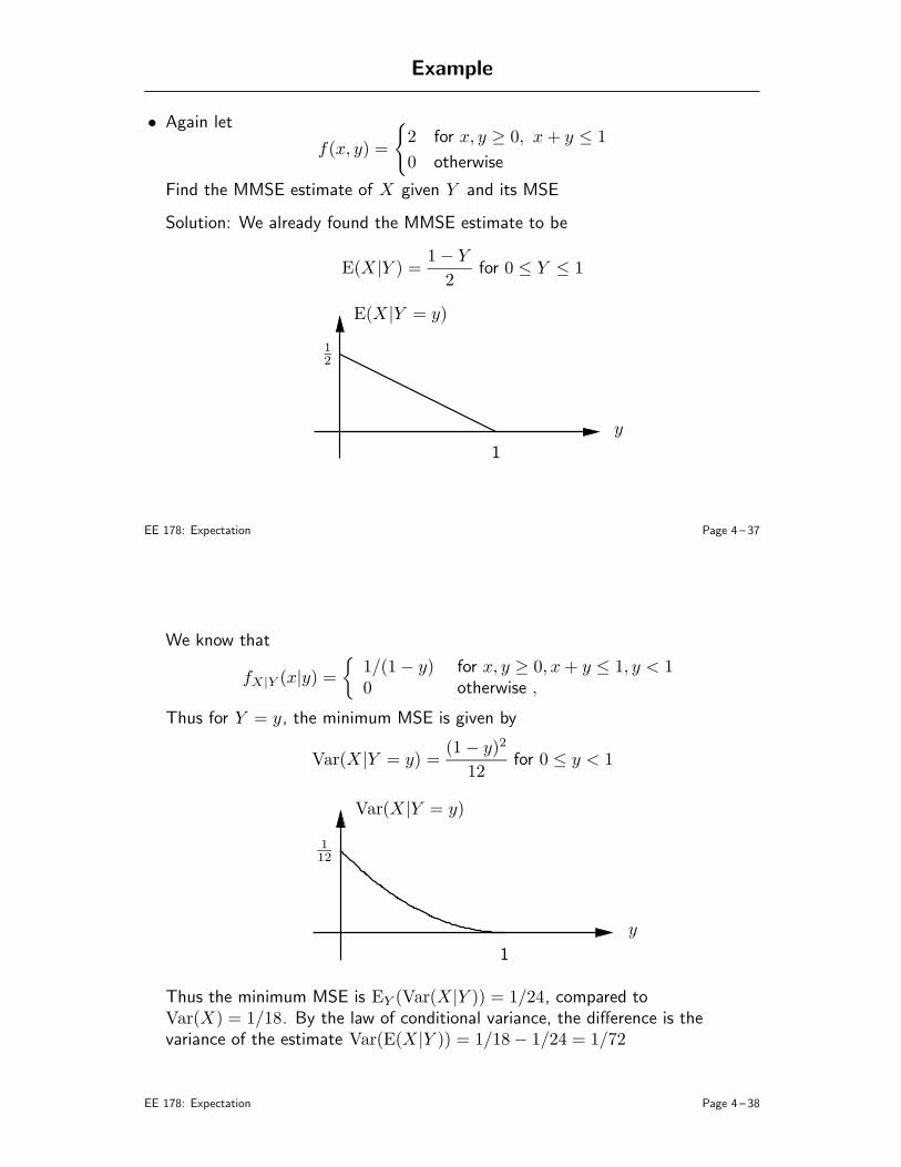
Example
• Again let
f(x, y) =
2 for x, y ≥ 0, x+ y ≤ 1
0 otherwise
Find the MMSE estimate of X given Y and its MSE
Solution: We already found the MMSE estimate to be
E(X |Y ) =1− Y
2for 0 ≤ Y ≤ 1
E(X |Y = y)
y
12
1
EE 178: Expectation Page 4 – 37
We know that
fX|Y (x|y) =
1/(1− y) for x, y ≥ 0, x+ y ≤ 1, y < 10 otherwise ,
Thus for Y = y, the minimum MSE is given by
Var(X |Y = y) =(1− y)2
12for 0 ≤ y < 1
Var(X |Y = y)
y
112
1
Thus the minimum MSE is EY (Var(X |Y )) = 1/24, compared toVar(X) = 1/18. By the law of conditional variance, the difference is thevariance of the estimate Var(E(X |Y )) = 1/18− 1/24 = 1/72
EE 178: Expectation Page 4 – 38
Sum of Random Number of Independent RVs
• Let N be a r.v. taking positive integer values and X1,X2, . . . be a sequence ofi.i.d. r.v.s independent of N
• Define the sum
Y =N∑
i=1
Xi
• We are given E(N), Var(N), the mean of Xi, E(X), and its variance Var(X)and wish to find the mean and variance of Y
• Using iterated expectation, the mean is:
EE 178: Expectation Page 4 – 39
E(Y ) = EN
[
E
(
N∑
i=1
Xi
∣
∣
∣N
)]
= EN
(
N∑
i=1
E(Xi|N)
)
by linearity of expectation
= EN
(
N∑
i=1
E(Xi)
)
Xi and Nareindependent
= EN [N E(X)] = E(N) E(X)
Using the law of conditional variance, the variance is:
Var(Y ) = E [Var(Y |N)] + Var(E(Y |N))
= E [NVar(X)] + Var(N E(X))
= Var(X)E(N) + (E(X))2Var(N)
• Example: You visit bookstores looking for a copy of the Great Expectations.
EE 178: Expectation Page 4 – 40
Each bookstore carries the book with probability p, independent of all otherbookstores. You keep visiting bookstores until you find the book. In eachbookstore visited, you spend a random amount of time, exponentially distributedwith parameter λ. Assuming that you will keep visiting bookstores until you buythe book and that the time spent in each is independent of everything else, findthe mean and variance of the total time spent in bookstores.
EE 178: Expectation Page 4 – 41
Solution: The total number of bookstores visited is a r.v. N ∼ Geom(p). LetXi be the amount of time spent in each bookstore. Thus, X1, X2, . . . are i.i.d.Exp(λ) r.v.s. Now let Y be the total amount of time spent looking for thebooks. Then
Y =N∑
i=1
Xi
The mean and variance of Y , thus, are
E(Y ) = E(N) E(X) =1
pλ
Var(Y ) = Var(X)E(N) + (E(X))2Var(N)
=1
pλ2+
1
λ2×
1− p
p2=
1
p2λ2
EE 178: Expectation Page 4 – 42
Lecture Notes 5
Transforms
• Definition
• Examples
• Moment Generating Properties
• Inversion
• Transforms of Sums of Independent RVs
Corresponding pages from B&T: 210–219, 232–236.
EE 178: Transforms Page 5 – 1
Definition
• The transform associated with the probability distribution of a random variableX is defined as
MX(s) = E(
esX)
=
∑
x esxpX(x), for X ∼ pX(x)
∫
∞
−∞esxfX(x) dx, for X ∼ fX(x),
where s is a scalar parameter
• Closely related to Fourier, Laplace and z transforms (depends on allowed valuesof s)
• When we use s, the transform is called the moment generating function. Whenwe plug s = iω, where i =
√−1 and ω is a real-valued parameter, the
transform is called the characteristic function
• Important fact: There is a one-to-one correspondence between the momentgenerating function for a r.v. and its probability distribution (pmf or pdf)
EE 178: Transforms Page 5 – 2
Moment Generating Function: Examples
• X ∼ Bern(p): pX(1) = p, pX(0) = 1− p
MX(s) = E(
esX)
=
1∑
k=0
eskpX(k) = (1− p) + pes
• X ∼ Geom(p): pX(k) = p(1− p)k−1, k = 1, 2, . . .
MX(s) = E(
esX)
=∞∑
k=1
pX(k)esk
=
∞∑
k=1
p(1− p)k−1esk
= pes∞∑
k=0
((1− p)es)k =pes
1− (1− p)es,
provided (1− p)es < 1, which implies that s < ln(1/(1− p))
Note: In general, MX(s) is defined only over values of s where it is finite
EE 178: Transforms Page 5 – 3
• X ∼ Poisson(λ): pX(k) = λk
k! e−λ, k ≥ 0
MX(s) = E(
esX)
=∞∑
k=0
eskλk
k!e−λ
= e−λ∞∑
k=0
ak
k!, where a = λes
= e−λ × ea = eλ(es−1)
• X ∼ Exp(λ): fX(x) = λe−λx, x ≥ 0
MX(s) = E(
esX)
=
∫
∞
0
λe−λxesx dx =λ
λ− s
for s < λ
EE 178: Transforms Page 5 – 4
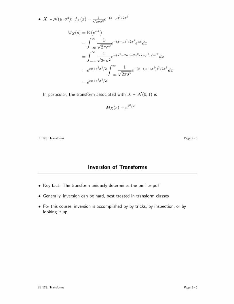
• X ∼ N (µ, σ2): fX(x) = 1√
2πσ2e−(x−µ)2/2σ2
MX(s) = E(
esX)
=
∫
∞
−∞
1√2πσ2
e−(x−µ)2/2σ2esx dx
=
∫
∞
−∞
1√2πσ2
e−(x2−2µx−2σ2sx+µ2)/2σ2
dx
= esµ+s2σ2/2
∫
∞
−∞
1√2πσ2
e−(x−(µ+sσ2))2/2σ2dx
= esµ+s2σ2/2
In particular, the transform associated with X ∼ N (0, 1) is
MX(s) = es2/2
EE 178: Transforms Page 5 – 5
Inversion of Transforms
• Key fact: The transform uniquely determines the pmf or pdf
• Generally, inversion can be hard, best treated in transform classes
• For this course, inversion is accomplished by by tricks, by inspection, or bylooking it up
EE 178: Transforms Page 5 – 6
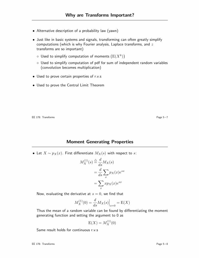
Why are Transforms Important?
• Alternative description of a probability law (yawn)
• Just like in basic systems and signals, transforming can often greatly simplifycomputations (which is why Fourier analysis, Laplace transforms, and ztransforms are so important)
Used to simplify computation of moments (E(Xk))
Used to simplify computation of pdf for sum of independent random variables(convolution becomes multiplication)
• Used to prove certain properties of r.v.s
• Used to prove the Central Limit Theorem
EE 178: Transforms Page 5 – 7
Moment Generating Properties
• Let X ∼ pX(x). First differentiate MX(s) with respect to s:
M(1)X (s)
=d
dsMX(s)
=d
ds
∑
x
pX(x)esx
=∑
x
xpX(x)esx
Now, evaluating the derivative at s = 0, we find that
M(1)X (0) =
d
dsMX(s)
∣
∣
∣
s=0= E(X)
Thus the mean of a random variable can be found by differentiating the momentgenerating function and setting the argument to 0 as
E(X) = M(1)X (0)
Same result holds for continuous r.v.s
EE 178: Transforms Page 5 – 8
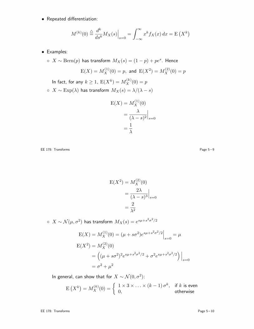
• Repeated differentiation:
M (k)(0)
=dk
dskMX(s)
∣
∣
∣
s=0=
∫
∞
−∞
xkfX(x) dx = E(
Xk)
• Examples:
X ∼ Bern(p) has transform MX(s) = (1− p) + pes. Hence
E(X) = M(1)X (0) = p, and E(X2) = M
(2)X (0) = p
In fact, for any k ≥ 1, E(Xk) = M(k)X (0) = p
X ∼ Exp(λ) has transform MX(s) = λ/(λ− s)
E(X) = M(1)X (0)
=λ
(λ− s)2
∣
∣
∣
s=0
=1
λ
EE 178: Transforms Page 5 – 9
E(X2) = M(2)X (0)
=2λ
(λ− s)3
∣
∣
∣
s=0
=2
λ2
X ∼ N (µ, σ2) has transform MX(s) = esµ+s2σ2/2
E(X) = M(1)X (0) = (µ+ sσ2)esµ+s2σ2/2
∣
∣
∣
s=0= µ
E(X2) = M(2)X (0)
=(
(µ+ sσ2)2esµ+s2σ2/2 + σ2esµ+s2σ2/2)∣
∣
∣
s=0
= σ2 + µ2
In general, can show that for X ∼ N (0, σ2):
E(
Xk)
= M(k)X (0) =
1× 3× . . .× (k − 1)σk, if k is even0, otherwise
EE 178: Transforms Page 5 – 10
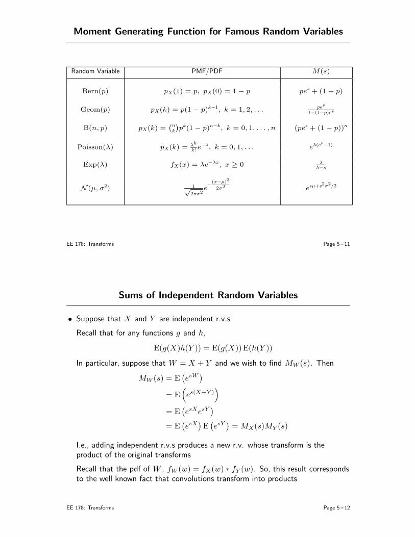
Moment Generating Function for Famous Random Variables
Random Variable PMF/PDF M(s)
Bern(p) pX(1) = p, pX(0) = 1 − p pes + (1 − p)
Geom(p) pX(k) = p(1 − p)k−1, k = 1, 2, . . . pes
1−(1−p)es
B(n, p) pX(k) =(nk
)
pk(1 − p)n−k, k = 0, 1, . . . , n (pes + (1 − p))n
Poisson(λ) pX(k) = λk
k! e−λ, k = 0, 1, . . . eλ(e
s−1)
Exp(λ) fX(x) = λe−λx, x ≥ 0 λλ−s
N (µ, σ2) 1√
2πσ2e−(x−µ)2
2σ2 esµ+s2σ2/2
EE 178: Transforms Page 5 – 11
Sums of Independent Random Variables
• Suppose that X and Y are independent r.v.s
Recall that for any functions g and h,
E(g(X)h(Y )) = E(g(X)) E(h(Y ))
In particular, suppose that W = X + Y and we wish to find MW (s). Then
MW (s) = E(
esW)
= E(
es(X+Y ))
= E(
esXesY)
= E(
esX)
E(
esY)
= MX(s)MY (s)
I.e., adding independent r.v.s produces a new r.v. whose transform is theproduct of the original transforms
Recall that the pdf of W , fW (w) = fX(w) ∗ fY (w). So, this result correspondsto the well known fact that convolutions transform into products
EE 178: Transforms Page 5 – 12
• This result can be extended to more than 2 r.v.s:
Let X1, X2, . . . , Xn be mutually independent random variables with momentgenerating functions MX1,MX2, . . . ,MXn, respectively, then the momentgenerating function of their sum Y =
∑ni=1Xi is
MY (s) =n∏
i=1
MXi(s)
If the Xis are independent and identically distributed with a common momentgenerating function MX(s), then
MY (s) = (MX(s))n
• So to find the pdf of a sum of independent r.v.s you can either convolve theirpdfs or multiply their moment generating functions and then invert the result
EE 178: Transforms Page 5 – 13
Examples
• Moment generating function for a Binomial r.v.: Let Y ∼ B(n, p). We wish tofind its moment generating function MY (s)
Recall that we can express Y as a sum of n i.i.d. Bern(p) r.v.s,X1,X2, . . . ,Xn. Since the moment generating function of a Bern(p) r.v. is
MX(s) =
1∑
k=0
eskpX(k) = (1− p) + pes,
the moment generating function of the binomial r.v. Y =∑n
i=1Xi, is
MY (s) = ((1− p) + pes)n
To verify, let’s find the inverse. By the Newton expansion formula
((1− p) + pes)n =n∑
k=0
((
n
k
)
pk(1− p)n−k
)
esk
=n∑
k=0
pY (k)esk
EE 178: Transforms Page 5 – 14
• Suppose we have two independent Gaussian r.v.s, X ∼ N (µX, σ2X) and
Y ∼ N (µY , σ2Y ) and we wish to find the pdf of their sum W = X + Y
We first find the transform of their sum
MW (s) = MX(s)MY (s)
= esµX+s2σ2X/2esµY +s2σ2
Y /2
= es(µX+µY )+s2(σ2X+σ2
Y )/2
We now invert the tranform to find the pdf. This is very easy since the form ofthe transform is that of a Gaussian pdf with mean µX + µY and varianceσ2X + σ2
Y , i.e., W ∼ N (µX + µY , σ2X + σ2
Y )
So, if we add two (or more) independent Gaussian r.v.s, we obtain a Gaussianr.v.. This shows that Gaussian distribution is infinitely divisible (see LectureNotes 3)
EE 178: Transforms Page 5 – 15
Distribution of a Random Sum of RVs
• Let N be a r.v. taking positive integer values and X1,X2, . . . be a sequence ofi.i.d. r.v.s independent of N
• Define the sum
Y =N∑
i=1
Xi
• Using conditional expectation, we already found the mean and variance of Y interms of the mean and variance of X and N
• Now suppose we are given the transforms for X , MX(s), and N , MN(s), andwe wish to find the transform of Y . We again use conditional expectation
E(
esY | N = n)
= E(
esX1esX2 . . . esXN | N = n)
= E(
esX1esX2 . . . esXn)
= E(
esX1)
E(
esX2)
. . .E(
esXn)
= (MX(s))n
EE 178: Transforms Page 5 – 16
Using iterated expectation
MY (s) = E[
E(
esY | N)]
= E[
(MX(s))N]
Note the similarity between MY (s) above and
MN(s) = E(
esN)
They are the same except that MY replaces es in MN by MX(s). In otherwords, if we know the functional form of MN(s) and it depends on s onlythrough es, then we can find MY by simply replacing es by MX(s)
• Example: Recall the bookstore problem. N ∼ Geom(p) is the number of storesvisited and X1,X2, . . . are i.i.d. Exp(λ) r.v.s and represent the times spent ineach store. The total amount of time spent looking for the book until it’s foundis
Y =N∑
i=1
Xi
Find the pdf of Y
EE 178: Transforms Page 5 – 17
Solution: We find the transform associated with Y and then invert it to find thepdf. First note that the transform for N is
MN(s) =pes
1− (1− p)es
Thus, the transform for Y is
MY (s) = E[
(MX(s))N]
=pMX(s)
1− (1− p)MX(s)
But, since X ∼ Exp(λ), its transform is
MX(s) =λ
λ− s
Substituting, we obtain
MY (s) =p(
λλ−s
)
1− (1− p)(
λλ−s
) =pλ
pλ− s
Thus, Y ∼ Exp(pλ)!
EE 178: Transforms Page 5 – 18
Lecture Notes 6
Limit Theorems
• Motivation
• Markov and Chebyshev Inequalities
• Weak Law of Large Numbers
• The Central Limit Theorem
• Confidence Intervals
Corresponding pages from B&T: 380–385, 388–392.
EE 178: Limit Theorems Page 6 – 1
Motivation
• One of the key questions in statistics is how to estimate the statistics of a r.v.,e.g., its mean, variance, distribution, etc.
• To estimate such a statistic, we collect samples and use an estimator in the formof a sample average
How good is the estimator? Does it “converge” to the true statistic?
How many samples do we need to ensure with some confidence that we arewithin a certain range of the true value of the statistic?
• These questions are answered using probability theory. The answers are calledlimit theorems
• Example: Suppose we are given a coin with unknown bias p. To estimate thebias we flip the coin n times and compute the relative frequency of occurrenceof heads nH/n.
Does nH/n → p?
How many coin flips do we need?
EE 178: Limit Theorems Page 6 – 2
The Sample Mean
• We can cast the above example as an example of estimating the mean of a r.v..Suppose X is a r.v. with finite but unknown mean E(X) (e.g., for the coinflipping example X ∼ Bern(p) and we want to estimate E(X) = p)
• To estimate the mean, we collect X1,X2, . . . ,Xn i.i.d. samples drawn accordingto the same distribution as X and compute the sample mean
Sn =1
n
n∑
i=1
Xi
Does Sn → E(X) as n → ∞?
What do we mean by convergence here?
How large should n be?
EE 178: Limit Theorems Page 6 – 3
• Mean and variance of Sn: From previous discussions we know that
E (Sn) =1
n
n∑
i=1
E(Xi) = E(X)
Var (Sn) =1
n2Var
(
n∑
i=1
Xi
)
= σ2X/n
• Thus,
Var (Sn) = E[
(Sn − E(Sn))2]
= E[
(Sn − E(X))2]
→ 0, as n → ∞
• This result is an example of limit theorem. It says that the sample meanconverges in mean square to the true mean of the r.v.
• We will prove another limit theorem called the Weak Law of Large Numbers
using this result
• We then answer the question of how many samples are needed using the Central
Limit Theorem
EE 178: Limit Theorems Page 6 – 4
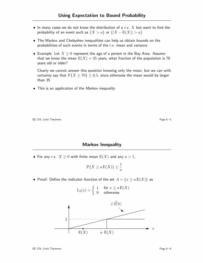
Using Expectation to Bound Probability
• In many cases we do not know the distribution of a r.v. X but want to find theprobability of an event such as X > a or |X − E(X)| > a
• The Markov and Chebyshev inequalities can help us obtain bounds on theprobabilities of such events in terms of the r.v. mean and variance
• Example: Let X ≥ 0 represent the age of a person in the Bay Area. Assumethat we know the mean E(X) = 35 years, what fraction of the population is 70years old or older?
Clearly we cannot answer this question knowing only the mean, but we can withcertainty say that PX ≥ 70 ≤ 0.5, since otherwise the mean would be largerthan 35
• This is an application of the Markov inequality
EE 178: Limit Theorems Page 6 – 5
Markov Inequality
• For any r.v. X ≥ 0 with finite mean E(X) and any a > 1,
PX ≥ aE(X) ≤1
a
• Proof: Define the indicator function of the set A = x ≥ aE(X) as
IA(x) =
1 for x ≥ aE(X)0 otherwise
x
1
E(X) a.E(X)
xa.E(X)
EE 178: Limit Theorems Page 6 – 6
From the figure it follows that
IA(X) ≤X
aE(X)
Taking the expectation of both sides, we obtain the Markov inequality
E(IA(X)) = PX ≥ aE(X) ≤ E (X/aE(X)) = 1/a
• The Markov inequality can be very loose. Let X ∼ Exp(1), then
PX ≥ 10 = e−10 ≈ 4.54× 10⁻⁵
The Markov inequality gives
PX ≥ 10 ≤1
10,
which is very pessimistic
EE 178: Limit Theorems Page 6 – 7
Chebyshev Inequality
• Let X be a device parameter in an integrated circuit (IC) with known mean andvariance. The IC is out-of-spec if X is more than, say, 3σX away from its mean.We wish to find the fraction of out-of-spec ICs, P|X − E(X)| ≥ 3σX
• The Chebyshev inequality gives us an upper bound on this fraction in terms themean and variance of X
• Let X be a r.v. with finite mean E(X) and variance σ2X . The Chebyshev
inequality states that for any a > 1
P|X − E(X)| ≥ aσX ≤1
a2
• Proof: We use the Markov inequality. Define the r.v. Y = (X − E(X))2 ≥ 0.Since E(Y ) = σ2
X , the Markov inequality gives
PY ≥ a2σ2X ≤
1
a2
EE 178: Limit Theorems Page 6 – 8
But|X − E(X)| ≥ aσX occurs iff Y ≥ a2σ2
X
Thus
P|X − E(X)| ≥ aσX ≤1
a2
• The Chebyshev inequality can be very loose. Let X ∼ N (0, 1). Using theChebyshev inequality, we obtain
P|X | ≥ 3 ≤1
9,
which is very pessimistic compared to the actual value ≈ 2× 10⁻³
EE 178: Limit Theorems Page 6 – 9
The Weak Law of Large Numbers
• The WLLN states that if X1,X2, . . . ,Xn is a sequence of i.i.d. r.v.s with finitemean E(X) and variance σ2
X , then for any ǫ > 0,
limn→∞
P|Sn − E(X)| > ǫ = 0
• Proof: By the Chebyshev inequality
P|Sn − E(Sn)| > ǫ ≤Var(Sn)
ǫ2
But, E(Sn) = E(X) and Var(Sn) = σ2X/n, thus
P|Sn − E(X)| > ǫ ≤σ2X
nǫ2→ 0, as n → ∞
• Note that the WLLN holds if X1,X2, . . . ,Xn are only pairwise independent,which is weaker than mutual independence.In fact, we only need the r.v.s to be uncorrelated, which is in general evenweaker than pairwise independence
EE 178: Limit Theorems Page 6 – 10
Confidence Intervals
• Given ǫ, δ > 0, how large should the number of samples n be such that
P|Sn − E(X)| ≤ ǫ ≥ 1− δ,
i.e., with probability ≥ (1− δ), Sn is within ± ǫ of E(X)
• Let’s use the Chebyshev inequality
P|Sn − E(X)| ≤ ǫ = P|Sn − E(Sn)| ≤ ǫ
= 1− P|Sn − E(Sn)| > ǫ
≥ 1−Var(Sn)
ǫ2= 1−
σ2X
nǫ2
So if we let σ2X/nǫ2 ≤ δ, we obtain n ≥ σ2
X/δǫ2
• Example: Let ǫ = 0.1σX and δ = .001, then the number of samplesn ≥ σ2
X/10−2σ2X10−3 = 105, i.e., 105 samples ensure that Sn is within ±0.1σX
of E(X) with probability (confidence) of 0.999 or better, independent of thedistribution of X
EE 178: Limit Theorems Page 6 – 11
• The Pollster’s Problem: Let p be the fraction of people that intend to vote forSnidely Whiplash against Dudley Doright. A pollester polls n people.
For the i th person polled define the r.v.
Xi =
1 prefers Whiplash0 otherwise
Let Sn = 1n
∑ni=1Xi be the sample mean of the Xis, i.e., the fraction of people
polled that prefer Whiplash
The pollster wants to choose n large enough to ensure that
P|Sn − p| ≤ .01 ≥ 0.95
• Solution: By the Chebyshev inequality,
P|Sn − p| ≤ .01 ≥ 1−σ2X
n(0.01)2
But, X ∼ Bern(p), thus σ2X = p(1− p) ≤ 0.25. Thus n = 50, 000 suffices (as
we shall see, 50, 000 is wildly conservative)
EE 178: Limit Theorems Page 6 – 12
Gaussian Random Variables
• A Gaussian random variable X ∼ N (µ, σ2), has the pdf
fX(x) =1
√2πσ2
e−
(x−µ)2
2σ2
• Gaussian has several nice properties:
If Y = aX + b, then Y ∼ N (aµ+ b, a2σ2)
The transform closely resembles the form of the pdf: MX(s) = esµ+s2σ2/2
If X1, X2, . . . , Xn are independent and Xi ∼ N (µi, σ2i ), for i = 1, 2, . . . , n,
then W =∑
i aiXi ∼ N(∑
i aiµi,∑
i a2iσ
2i
)
In particular, any weighted sum of i.i.d. Gaussian r.v.s is Gaussian
• We shall see that a certain weighted sum of i.i.d. r.v.s is approximately Gaussianeven when the r.v.s themselves are not Gaussian — a result known as theCentral Limit Theorem (CLT)
An important reason for the great popularity of Gaussian models
EE 178: Limit Theorems Page 6 – 13
The Standardized Sum
• Let X1, X2, . . . , Xn be a sequence of i.i.d. r.v.s with finite mean E(X) andvariance σ2
X
• We define the “standardized” or “normalized” sum
Zn =1√n
n∑
k=1
(
Xk − E(X)
σX
)
• Zn is called “standardized” because E(Zn) = 0, and σ2Zn
= 1
• In the special case where E(X) = 0 and σ2X = 1, the standardized sum becomes
Zn =1√n
n∑
k=1
Xk
Note the similarity to the sample average Sn considered for the law of largenumbers: Zn =
√nSn
EE 178: Limit Theorems Page 6 – 14
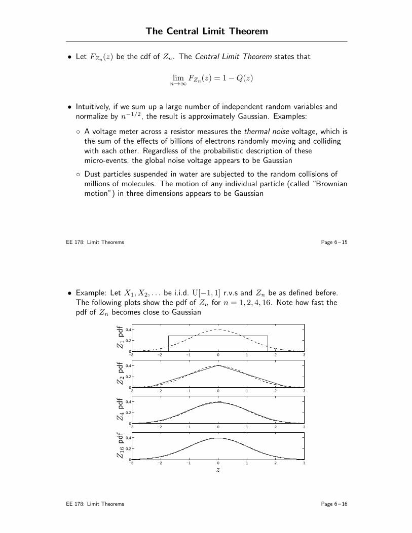
The Central Limit Theorem
• Let FZn(z) be the cdf of Zn. The Central Limit Theorem states that
limn→∞
FZn(z) = 1−Q(z)
• Intuitively, if we sum up a large number of independent random variables andnormalize by n−1/2, the result is approximately Gaussian. Examples:
A voltage meter across a resistor measures the thermal noise voltage, which isthe sum of the effects of billions of electrons randomly moving and collidingwith each other. Regardless of the probabilistic description of thesemicro-events, the global noise voltage appears to be Gaussian
Dust particles suspended in water are subjected to the random collisions ofmillions of molecules. The motion of any individual particle (called “Brownianmotion”) in three dimensions appears to be Gaussian
EE 178: Limit Theorems Page 6 – 15
• Example: Let X1,X2, . . . be i.i.d. U[−1, 1] r.v.s and Zn be as defined before.The following plots show the pdf of Zn for n = 1, 2, 4, 16. Note how fast thepdf of Zn becomes close to Gaussian
−3 −2 −1 0 1 2 30
0.2
0.4
−3 −2 −1 0 1 2 30
0.2
0.4
−3 −2 −1 0 1 2 30
0.2
0.4
−3 −2 −1 0 1 2 30
0.2
0.4
z
Z1pdf
Z2pdf
Z4pdf
Z16pdf
EE 178: Limit Theorems Page 6 – 16
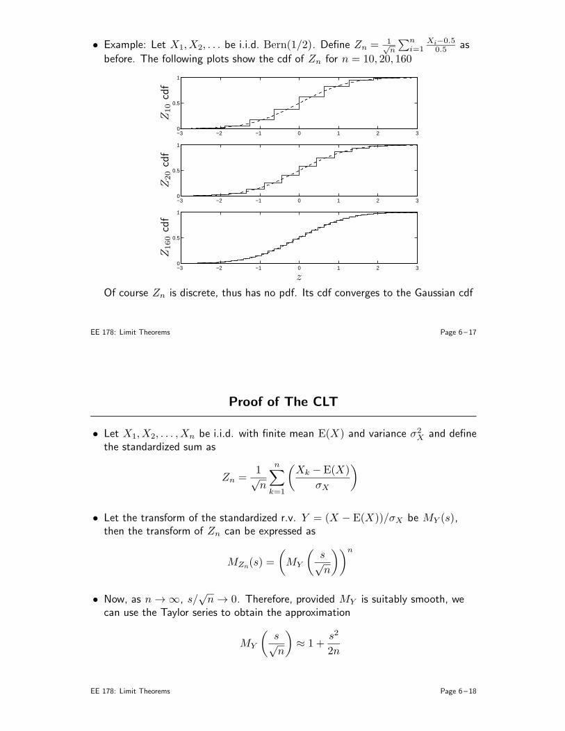
• Example: Let X1,X2, . . . be i.i.d. Bern(1/2). Define Zn = 1√
n
∑ni=1
Xi−0.50.5 as
before. The following plots show the cdf of Zn for n = 10, 20, 160
−3 −2 −1 0 1 2 30
0.5
1
−3 −2 −1 0 1 2 30
0.5
1
−3 −2 −1 0 1 2 30
0.5
1
z
Z10cdf
Z20cdf
Z160cdf
Of course Zn is discrete, thus has no pdf. Its cdf converges to the Gaussian cdf
EE 178: Limit Theorems Page 6 – 17
Proof of The CLT
• Let X1,X2, . . . ,Xn be i.i.d. with finite mean E(X) and variance σ2X and define
the standardized sum as
Zn =1√n
n∑
k=1
(
Xk − E(X)
σX
)
• Let the transform of the standardized r.v. Y = (X − E(X))/σX be MY (s),then the transform of Zn can be expressed as
MZn(s) =
(
MY
(
s√n
))n
• Now, as n → ∞, s/√n → 0. Therefore, provided MY is suitably smooth, we
can use the Taylor series to obtain the approximation
MY
(
s√n
)
≈ 1 +s2
2n
EE 178: Limit Theorems Page 6 – 18
Proof: To see why, recall that the Taylor series of a function f(u) around thepoint u = 0 has the form
f(u) =∞∑
k=0
ukf(k)(0)
k!
= f(0) + uf (1)(0) + u2f(2)(0)
2+ o(u2),
where o(u2) → 0 faster than u2 and the derivatives
f (k)(0) =dk
dukf(u)
∣
∣
∣
u=0
are assumed to exist
EE 178: Limit Theorems Page 6 – 19
Combining the Taylor series expansion with the moment-generating property ofthe transform for a r.v. Y yields
MY (s) =
∞∑
k=0
skM
(k)Y (0)
k!
=∞∑
k=0
skE(
Y k)
k!
= 1 + sE(Y ) +s2
2E(Y 2) + o(s2)
Now, replacing s by s/√n, we obtain
MY
(
s√n
)
≈ 1 +s2
2n,
as claimed
EE 178: Limit Theorems Page 6 – 20
• Hence
limn→∞
MZn(s) = limn→∞
(
1 +s2
2n
)n
= es2/2
So asymptotically the transform of Zn looks like that for a N (0, 1) r.v.
• The CLT follows from this result and the following fact:If the sequence of transforms MZn(s) converges to a transform MZ(s) of a r.v.Z whose cdf is continuous, then the sequence of cdfs FZn converges to the cdfof Z
The proof of this fact is beyond the scope of this course
EE 178: Limit Theorems Page 6 – 21
Confidence Intervals Revisited
• Let X1, X2, . . . , Xn be i.i.d. with finite mean E(X) and variance σ2X and Sn be
the sample mean
• Given ǫ, δ > 0, how large should the number of samples n be such that
P|Sn − E(X)| ≤ ǫ ≥ 1− δ,
• Let’s use the CLT to find an estimate of n. Consider:
P|Sn − E(X)| ≤ ǫ = P
∣
∣
∣
∣
∣
1
n
n∑
i=1
(Xi − E(X))
∣
∣
∣
∣
∣
≤ ǫ
= P
∣
∣
∣
∣
∣
1√n
n∑
i=1
(
Xi − E(X)
σX
)
∣
∣
∣
∣
∣
≤ǫ√n
σX
≈ 1− 2Q
(
ǫ√n
σX
)
EE 178: Limit Theorems Page 6 – 22
• Example: For ǫ = 0.1σX and δ = .001, we set 2Q(0.1√n) = .001, which gives
0.1√n = 3.3, or n = 1089 (<< 105, the bound using Chebyshev inequality)
• Example: The Pollster’s Problem Revisited
Recall that p is the fraction of the population that intend to vote for SnidelyWhiplash against Dudley Doright. For the i th person polled
Xi =
1 prefers Whiplash0 otherwise
Sn is the sample average of the Xis
The pollster wants to choose n large enough to ensure that
P|Sn − p| ≤ 0.01 ≥ 0.95
Before, we used Chebyshev inequality to obtain
P|Sn − p| ≤ 0.01 ≥ 1−σ2X
n(0.01)2
and concluded that n = 50, 000 suffices
EE 178: Limit Theorems Page 6 – 23
Now let’s use the CLT to approximate P|Sn − p| ≤ .01. Consider
P |Sn − p| ≤ 0.01 = P
∣
∣
∣
∣
∣
1
n
n∑
i=1
(Xi − E(X))
∣
∣
∣
∣
∣
≤ 0.01
= P
∣
∣
∣
∣
∣
1√n
n∑
i=1
(
Xi − E(X)
σX
)
∣
∣
∣
∣
∣
≤0.01
√n
σX
= P
|Zn| ≤0.01
√n
σX
Since σX ≤ 1/2,
P |Sn − p| ≤ .01 ≥ P
|Zn| ≤ 0.02√n
≈ 1− 2Q(
0.02√n)
Thus to have P|Sn − p| ≤ .01 ≥ 0.95, we set 2Q (0.02√n) = 0.05, which,
using the Q-function table, gives n ≈ 9604; a significantly better answer thanthe previous one
EE 178: Limit Theorems Page 6 – 24
Lecture Notes 7
Random Processes
• Definition
• IID Processes
• Bernoulli Process
Binomial Counting Process
Interarrival Time Process
• Markov Processes
• Markov Chains
Classification of States
Steady State Probabilities
Corresponding pages from B&T: 271–281, 313–340.
EE 178: Random Processes Page 7 – 1
Random Processes
• A random process (also called stochastic process) X(t) : t ∈ T is an infinitecollection of random variables, one for each value of time t ∈ T (or, in somecases distance)
• Random processes are used to model random experiments that evolve in time:
Received sequence/waveform at the output of a communication channel
Packet arrival times at a node in a communication network
Thermal noise in a resistor
Scores of an NBA team in consecutive games
Daily price of a stock
Winnings or losses of a gambler
Earth movement around a fault line
EE 178: Random Processes Page 7 – 2
Questions Involving Random Processes
• Dependencies of the random variables of the process:
How do future received values depend on past received values?
How do future prices of a stock depend on its past values?
How well do past earth movements predict an earthquake?
• Long term averages:
What is the proportion of time a queue is empty?
What is the average noise power generated by a resistor?
• Extreme or boundary events:
What is the probability that a link in a communication network is congested?
What is the probability that the maximum power in a power distribution lineis exceeded?
What is the probability that a gambler will lose all his capital?
EE 178: Random Processes Page 7 – 3
Discrete vs. Continuous-Time Processes
• The random process X(t) : t ∈ T is said to be discrete-time if the index setT is countably infinite, e.g., 1, 2, . . . or . . . ,−2,−1, 0,+1,+2, . . .:
The process is simply an infinite sequence of r.v.s X1,X2, . . .
An outcome of the process is simply a sequence of numbers
• The random process X(t) : t ∈ T is said to be continuous-time if the indexset T is a continuous set, e.g., (0,∞) or (−∞,∞)
The outcomes are random waveforms or random occurances in continuoustime
• We only discuss discrete-time random processes:
IID processes
Bernoulli process and associated processes
Markov processes
Markov chains
EE 178: Random Processes Page 7 – 4
IID Processes
• A process X1, X2, . . . is said to be independent and identically distributed (IID,or i.i.d.) if it consists of an infinite sequence of independent and identicallydistributed random variables
• Two important examples:
Bernoulli process: X1,X2, . . . are i.i.d. Bern(p), 0 < p < 1, r.v.s. Model forrandom phenomena with binary outcomes, such as:∗ Sequence of coin flips∗ Noise sequence in a binary symmetric channel∗ The occurrence of random events such as packets (1 corresponding to anevent and 0 to a non-event) in discrete-time
∗ Binary expansion of a random number between 0 and 1
Discrete-time white Gaussian noise (WGN) process: X1,X2, . . . are i.i.d.N (0, N) r.v.s. Model for:∗ Receiver noise in a communication system∗ Fluctuations in a stock price
EE 178: Random Processes Page 7 – 5
• Useful properties of an IID process:
Independence: Since the r.v.s in an IID process are independent, any twoevents defined on sets of random variables with non-overlapping indices areindependent
Memorylessness: The independence property implies that the IID process ismemoryless in the sense that for any time n, the future Xn+1,Xn+2, . . . isindependent of the past X1,X2, . . . ,Xn
Fresh start: Starting from any time n, the random process Xn, Xn+1, . . .behaves identically to the process X1, X2, . . ., i.e., it is also an IID processwith the same distribution. This property follows from the fact that the r.v.sare identically distributed (in addition to being independent)
EE 178: Random Processes Page 7 – 6
The Bernoulli Process
• The Bernoulli process is an infinite sequence X1,X2, . . . of i.i.d. Bern(p) r.v.s
• The outcome from a Bernoulli process is an infinite sequence of 0s and 1s
• A Bernoulli process is often used to model occurrences of random events;Xn = 1 if an event occurs at time n, and 0, otherwise
• Three associated random processes of interest:
Binomial counting process: The number of events in the interval [1, n]
Arrival time process: The time of event arrivals
Interarrival time process: The time between consecutive event arrivals
• We discuss these processes and their relationships
EE 178: Random Processes Page 7 – 7
Binomial Counting Process
• Consider a Bernoulli process X1, X2, . . . with parameter p
• We are often interested in the number of events occurring in some time interval
• For the time interval [1, n], i.e., i = 1, 2, . . . , n, we know that the number ofoccurrences
Wn =
(
n∑
i=1
Xi
)
∼ B(n, p)
• The sequence of r.v.s W1,W2, . . . is referred to as a Binomial counting process
• The Bernoulli process can be obtained from the Binomial counting process as:
Xn = Wn −Wn−1, for n = 1, 2, . . . ,
where W0 = 0
• Outcomes of a Binomial process are integer valued stair-case functions
EE 178: Random Processes Page 7 – 8
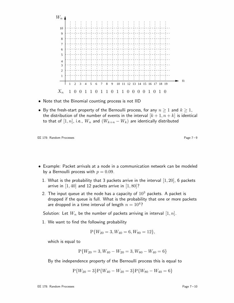
1 3 4 5 6 7 8 9 10 11 12 13 14 15 16 17 18 192
1
2
34
5
6
7
8
9
10
Wn
Xn
n
0000000000 1 11111111
• Note that the Binomial counting process is not IID
• By the fresh-start property of the Bernoulli process, for any n ≥ 1 and k ≥ 1,the distribution of the number of events in the interval [k + 1, n+ k] is identicalto that of [1, n], i.e., Wn and (Wk+n −Wk) are identically distributed
EE 178: Random Processes Page 7 – 9
• Example: Packet arrivals at a node in a communication network can be modeledby a Bernoulli process with p = 0.09.
1. What is the probability that 3 packets arrive in the interval [1, 20], 6 packetsarrive in [1, 40] and 12 packets arrive in [1, 80]?
2. The input queue at the node has a capacity of 103 packets. A packet isdropped if the queue is full. What is the probability that one or more packetsare dropped in a time interval of length n = 104?
Solution: Let Wn be the number of packets arriving in interval [1, n].
1. We want to find the following probability
PW20 = 3,W40 = 6,W80 = 12,
which is equal to
PW20 = 3,W40 −W20 = 3,W80 −W40 = 6
By the independence property of the Bernoulli process this is equal to
PW20 = 3PW40 −W20 = 3PW80 −W40 = 6
EE 178: Random Processes Page 7 – 10
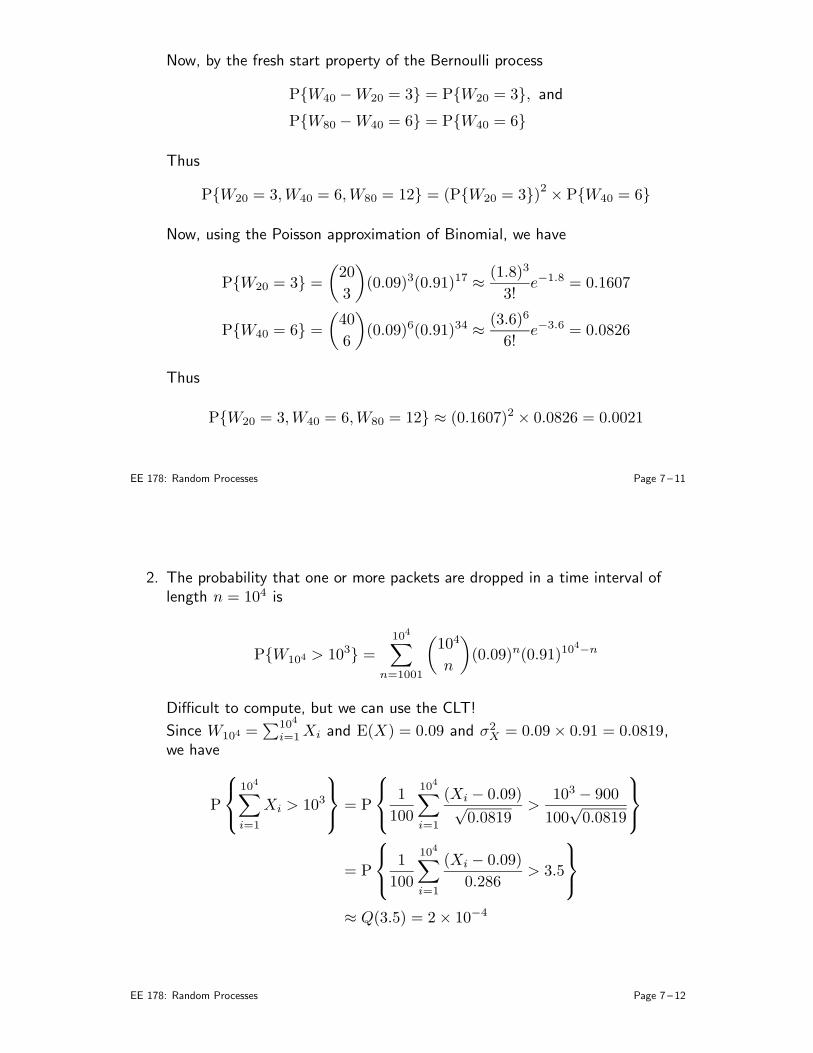
Now, by the fresh start property of the Bernoulli process
PW40 −W20 = 3 = PW20 = 3, and
PW80 −W40 = 6 = PW40 = 6
Thus
PW20 = 3,W40 = 6,W80 = 12 = (PW20 = 3)2× PW40 = 6
Now, using the Poisson approximation of Binomial, we have
PW20 = 3 =
(
20
3
)
(0.09)3(0.91)17 ≈(1.8)3
3!e−1.8 = 0.1607
PW40 = 6 =
(
40
6
)
(0.09)6(0.91)34 ≈(3.6)6
6!e−3.6 = 0.0826
Thus
PW20 = 3,W40 = 6,W80 = 12 ≈ (0.1607)2 × 0.0826 = 0.0021
EE 178: Random Processes Page 7 – 11
2. The probability that one or more packets are dropped in a time interval oflength n = 104 is
PW104 > 103 =104∑
n=1001
(
104
n
)
(0.09)n(0.91)104−n
Difficult to compute, but we can use the CLT!
Since W104 =∑104
i=1Xi and E(X) = 0.09 and σ2X = 0.09× 0.91 = 0.0819,
we have
P
104∑
i=1
Xi > 103
= P
1
100
104∑
i=1
(Xi − 0.09)√0.0819
>103 − 900
100√0.0819
= P
1
100
104∑
i=1
(Xi − 0.09)
0.286> 3.5
≈ Q(3.5) = 2× 10⁻⁴
EE 178: Random Processes Page 7 – 12
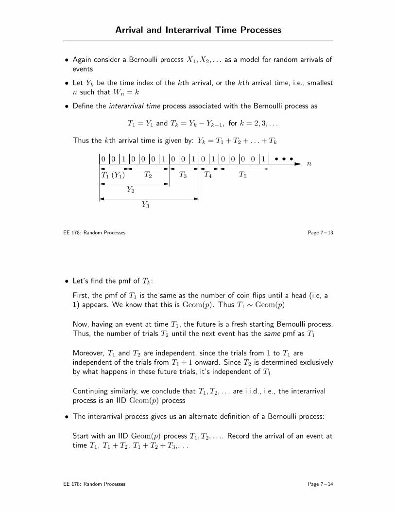
Arrival and Interarrival Time Processes
• Again consider a Bernoulli process X1,X2, . . . as a model for random arrivals ofevents
• Let Yk be the time index of the kth arrival, or the kth arrival time, i.e., smallestn such that Wn = k
• Define the interarrival time process associated with the Bernoulli process as
T1 = Y1 and Tk = Yk − Yk−1, for k = 2, 3, . . .
Thus the kth arrival time is given by: Yk = T1 + T2 + . . .+ Tk
000000000000 11111
T1 (Y1) T2 T3 T4 T5
Y2
Y3
n
EE 178: Random Processes Page 7 – 13
• Let’s find the pmf of Tk:
First, the pmf of T1 is the same as the number of coin flips until a head (i.e, a1) appears. We know that this is Geom(p). Thus T1 ∼ Geom(p)
Now, having an event at time T1, the future is a fresh starting Bernoulli process.Thus, the number of trials T2 until the next event has the same pmf as T1
Moreover, T1 and T2 are independent, since the trials from 1 to T1 areindependent of the trials from T1 + 1 onward. Since T2 is determined exclusivelyby what happens in these future trials, it’s independent of T1
Continuing similarly, we conclude that T1, T2, . . . are i.i.d., i.e., the interarrivalprocess is an IID Geom(p) process
• The interarrival process gives us an alternate definition of a Bernoulli process:
Start with an IID Geom(p) process T1, T2, . . .. Record the arrival of an event attime T1, T1 + T2, T1 + T2 + T3,. . .
EE 178: Random Processes Page 7 – 14
• Arrival time process: The sequence of r.v.s Y1, Y2, . . . is denoted by the arrivaltime process. From its relationship to the interarrival time process Y1 = T1,Yk =
∑ki=1 Ti, we can easily find the mean and variance of Yk for any k
E(Yk) = E
(
k∑
i=1
Ti
)
=k∑
i=1
E(Ti) = k ×1
p
Var(Yk) = Var
(
k∑
i=1
Ti
)
=
k∑
i=1
Var(Ti) = k ×1− p
p2
Note that, Y1, Y2, . . . is not an IID process
It is also not difficult to show that the pmf of Yk is
pYk(n) =
(
n− 1
k − 1
)
pk(1− p)n−k for n = k, k + 1, k + 2, . . . ,
which is called the Pascal pmf of order k
EE 178: Random Processes Page 7 – 15
• Example: In each minute of a basketball game, Alicia commits a foulindependently with probability p and no foul with probability 1− p. She stopsplaying if she commits her sixth foul or plays a total of 30 minutes. What is thepmf of of Alicia’s playing time?
Solution: We model the foul events as a Bernoulli process with parameter p
Let Z be the time Alicia plays. Then
Z = minY6, 30
The pmf of Y6 is
pY6(n) =
(
n− 1
5
)
p6(1− p)n−6, n = 6, 7, . . .
Thus the pmf of Z is
pZ(z) =
(
z−15
)
p6(1− p)z−6, for z = 6, 7, . . . , 29
1−∑29
z=6 pZ(z), for z = 30
0, otherwise
EE 178: Random Processes Page 7 – 16
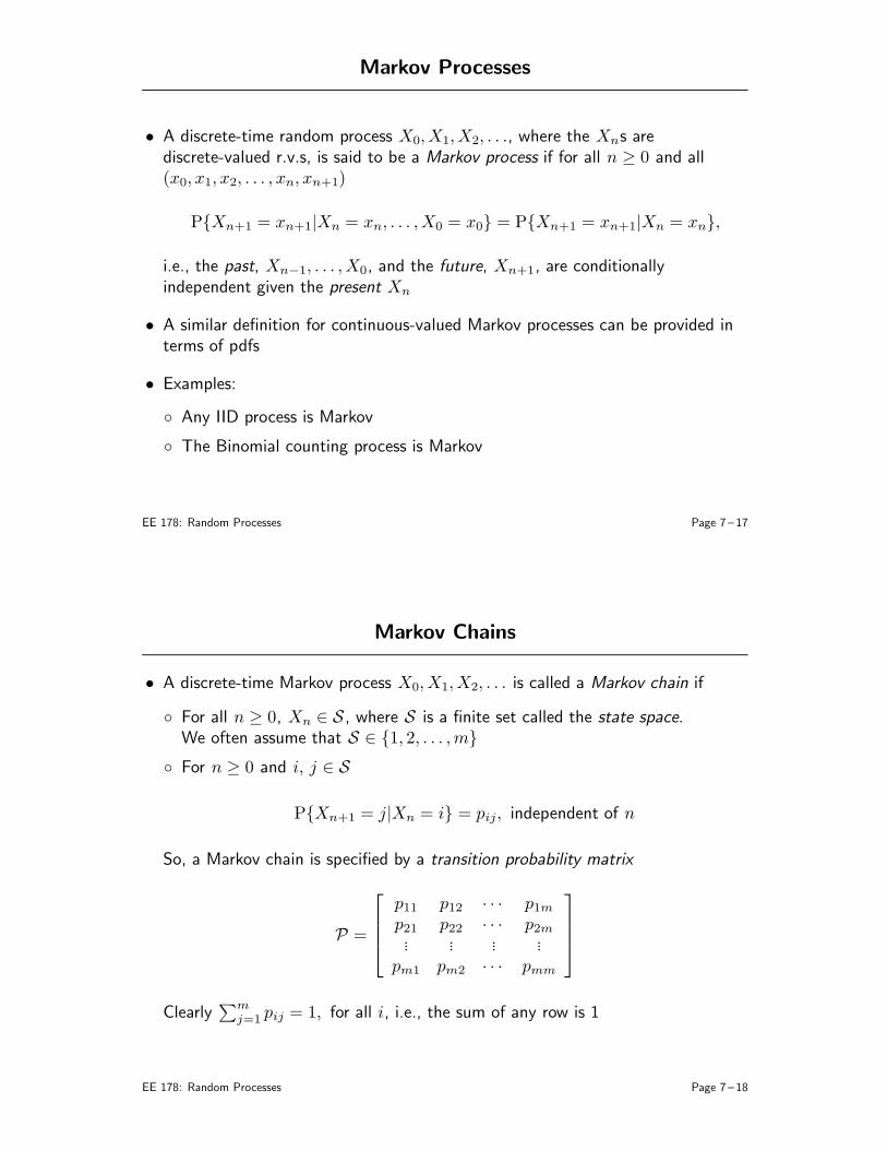
Markov Processes
• A discrete-time random process X0, X1, X2, . . ., where the Xns arediscrete-valued r.v.s, is said to be a Markov process if for all n ≥ 0 and all(x0, x1, x2, . . . , xn, xn+1)
PXn+1 = xn+1|Xn = xn, . . . ,X0 = x0 = PXn+1 = xn+1|Xn = xn,
i.e., the past, Xn−1, . . . , X0, and the future, Xn+1, are conditionallyindependent given the present Xn
• A similar definition for continuous-valued Markov processes can be provided interms of pdfs
• Examples:
Any IID process is Markov
The Binomial counting process is Markov
EE 178: Random Processes Page 7 – 17
Markov Chains
• A discrete-time Markov process X0, X1, X2, . . . is called a Markov chain if
For all n ≥ 0, Xn ∈ S , where S is a finite set called the state space.We often assume that S ∈ 1, 2, . . . ,m
For n ≥ 0 and i, j ∈ S
PXn+1 = j|Xn = i = pij, independent of n
So, a Markov chain is specified by a transition probability matrix
P =
p11 p12 · · · p1mp21 p22 · · · p2m... ... ... ...
pm1 pm2 · · · pmm
Clearly∑m
j=1 pij = 1, for all i, i.e., the sum of any row is 1
EE 178: Random Processes Page 7 – 18
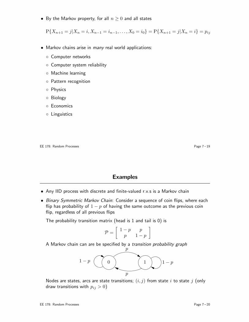
• By the Markov property, for all n ≥ 0 and all states
PXn+1 = j|Xn = i,Xn−1 = in−1, . . . , X0 = i0 = PXn+1 = j|Xn = i = pij
• Markov chains arise in many real world applications:
Computer networks
Computer system reliability
Machine learning
Pattern recognition
Physics
Biology
Economics
Linguistics
EE 178: Random Processes Page 7 – 19
Examples
• Any IID process with discrete and finite-valued r.v.s is a Markov chain
• Binary Symmetric Markov Chain: Consider a sequence of coin flips, where eachflip has probability of 1− p of having the same outcome as the previous coinflip, regardless of all previous flips
The probability transition matrix (head is 1 and tail is 0) is
P =
[
1− p pp 1− p
]
A Markov chain can are be specified by a transition probability graph
0 1
p
p
1− p 1− p
Nodes are states, arcs are state transitions; (i, j) from state i to state j (onlydraw transitions with pij > 0)
EE 178: Random Processes Page 7 – 20
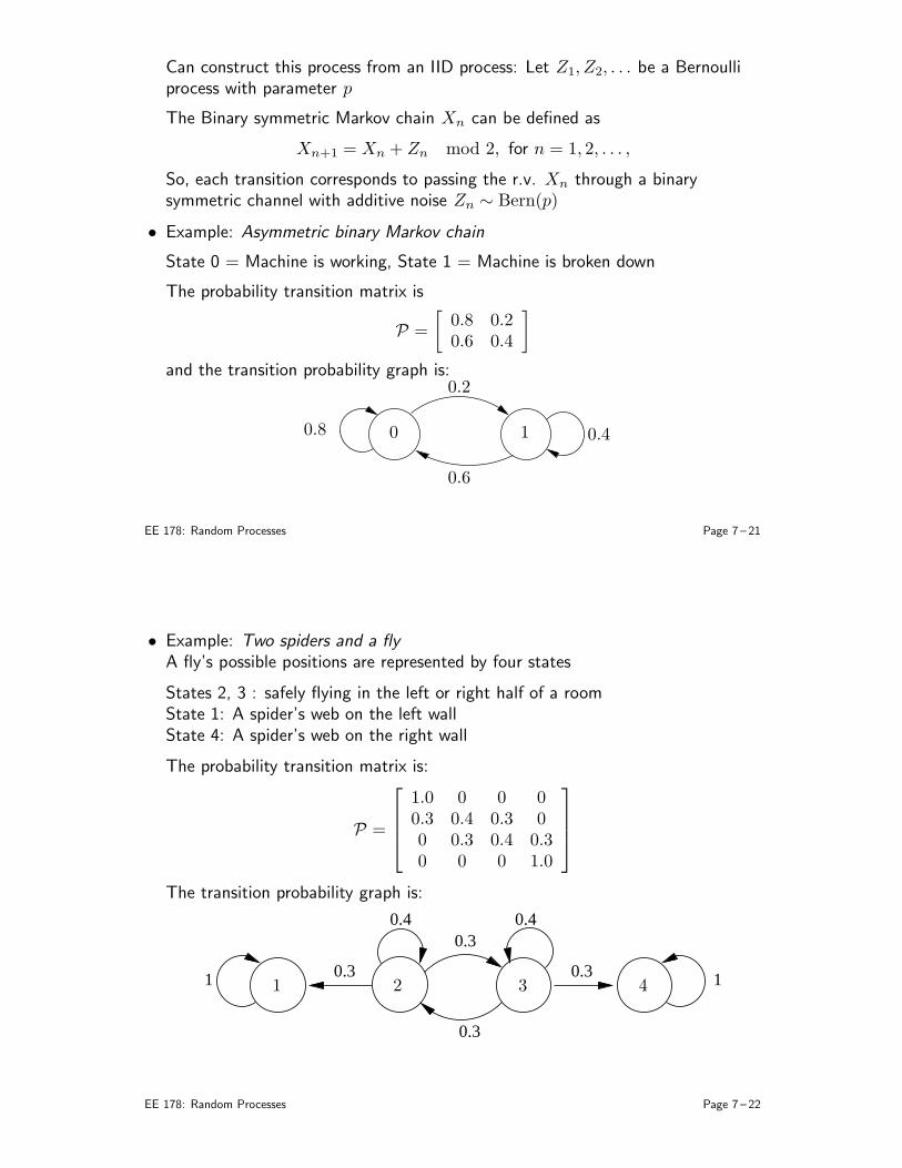
Can construct this process from an IID process: Let Z1, Z2, . . . be a Bernoulliprocess with parameter p
The Binary symmetric Markov chain Xn can be defined as
Xn+1 = Xn + Zn mod 2, for n = 1, 2, . . . ,
So, each transition corresponds to passing the r.v. Xn through a binarysymmetric channel with additive noise Zn ∼ Bern(p)
• Example: Asymmetric binary Markov chain
State 0 = Machine is working, State 1 = Machine is broken down
The probability transition matrix is
P =
[
0.8 0.20.6 0.4
]
and the transition probability graph is:
0 1
0.2
0.6
0.8 0.4
EE 178: Random Processes Page 7 – 21
• Example: Two spiders and a fly
A fly’s possible positions are represented by four states
States 2, 3 : safely flying in the left or right half of a roomState 1: A spider’s web on the left wallState 4: A spider’s web on the right wall
The probability transition matrix is:
P =
1.0 0 0 00.3 0.4 0.3 00 0.3 0.4 0.30 0 0 1.0
The transition probability graph is:
11
0.3
0.30.3
0.4 0.4
0.3
1 2 3 4
EE 178: Random Processes Page 7 – 22
• Given a Markov chain model, we can compute the probability of a sequence ofstates given an initial state X0 = i0 using the chain rule as:
PX1 = i1, X2 = i2, . . . ,Xn = in|X0 = i0 = pi0i1pi1i2 . . . pin−1in
Example: For the spider and fly example,
PX1 = 2,X2 = 2, X3 = 3|X0 = 2 = p22p22p23
= 0.4× 0.4× 0.3
= 0.048
• There are many other questions of interest, including:
n-state transition probabilities: Beginning from some state i what is theprobability that in n steps we end up in state j
Steady state probabilities: What is the expected fraction of time spent instate i as n → ∞?
EE 178: Random Processes Page 7 – 23
n-State Transition Probabilities
• Consider an m-state Markov Chain. Define the n-step transition probabilities as
rij(n) = PXn = j|X0 = i for 1 ≤ i, j ≤ m
• The n-step transition probabilities can be computed using theChapman-Kolmogorov recursive equation:
rij(n) =
m∑
k=1
rik(n− 1)pkj for n > 1, and all 1 ≤ i, j ≤ m,
starting with rij(1) = pij
This can be readily verified using the law of total probability
EE 178: Random Processes Page 7 – 24
• We can view the rij(n), 1 ≤ i, j ≤ m, as the elements of a matrix R(n), calledthe n-step transition probability matrix, then we can view theKolmogorov-Chapman equations as a sequence of matrix multiplications:
R(1) = P
R(2) = R(1)P = PP = P2
R(3) = R(2)P = P3
...
R(n) = R(n− 1)P = Pn
EE 178: Random Processes Page 7 – 25
• Example: For the binary asymmetric Markov chain
R(1) = P =
[
0.8 0.20.6 0.4
]
R(2) = P2 =
[
0.76 0.240.72 0.28
]
R(3) = P3 =
[
0.752 0.2480.744 0.256
]
R(4) = P4 =
[
0.7504 0.24960.7488 0.2512
]
R(5) = P5 =
[
0.7501 0.24990.7498 0.2502
]
In this example, each rij seems to converge to a non-zero limit independent ofthe initial state, i.e., each state has a steady state probability of being occupiedas n → ∞
EE 178: Random Processes Page 7 – 26
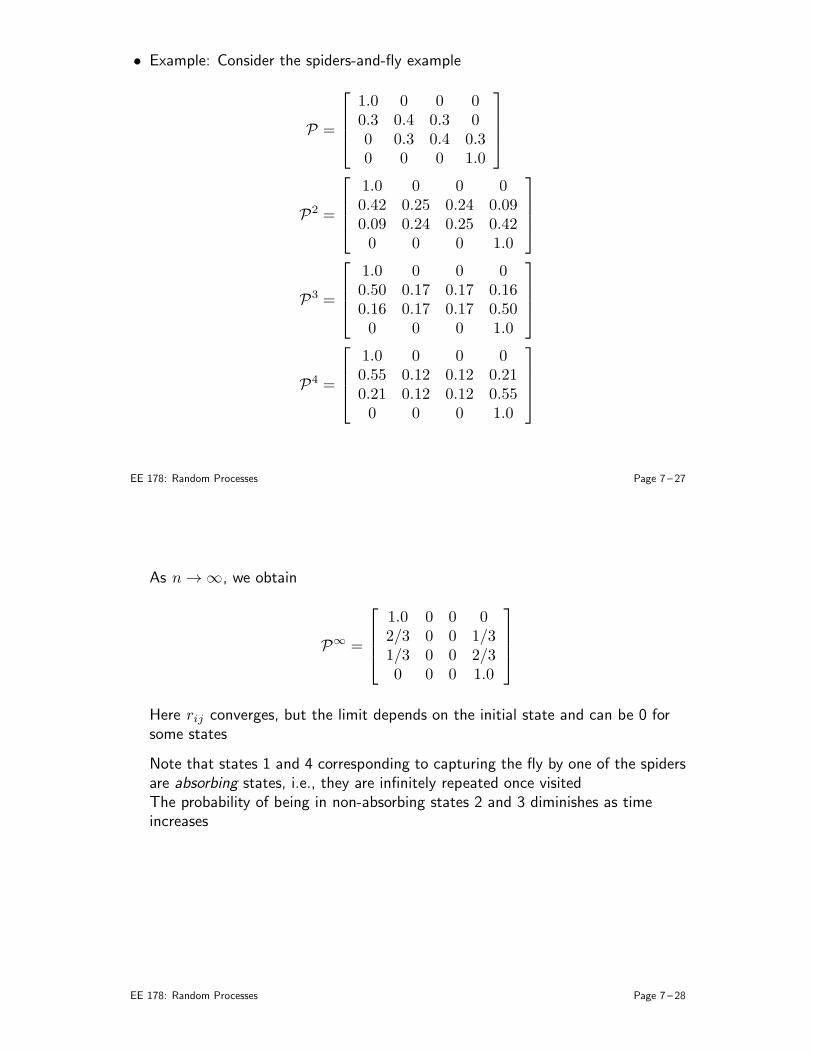
• Example: Consider the spiders-and-fly example
P =
1.0 0 0 00.3 0.4 0.3 00 0.3 0.4 0.30 0 0 1.0
P2 =
1.0 0 0 00.42 0.25 0.24 0.090.09 0.24 0.25 0.420 0 0 1.0
P3 =
1.0 0 0 00.50 0.17 0.17 0.160.16 0.17 0.17 0.500 0 0 1.0
P4 =
1.0 0 0 00.55 0.12 0.12 0.210.21 0.12 0.12 0.550 0 0 1.0
EE 178: Random Processes Page 7 – 27
As n → ∞, we obtain
P∞ =
1.0 0 0 02/3 0 0 1/31/3 0 0 2/30 0 0 1.0
Here rij converges, but the limit depends on the initial state and can be 0 forsome states
Note that states 1 and 4 corresponding to capturing the fly by one of the spidersare absorbing states, i.e., they are infinitely repeated once visitedThe probability of being in non-absorbing states 2 and 3 diminishes as timeincreases
EE 178: Random Processes Page 7 – 28
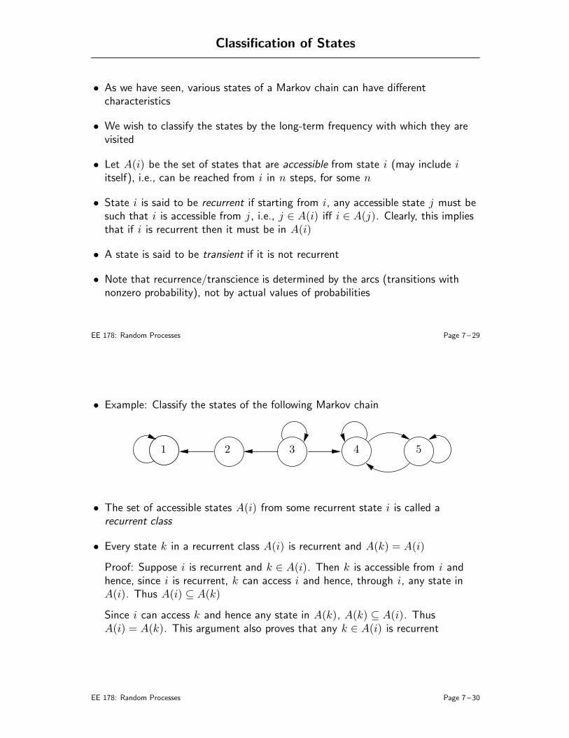
Classification of States
• As we have seen, various states of a Markov chain can have differentcharacteristics
• We wish to classify the states by the long-term frequency with which they arevisited
• Let A(i) be the set of states that are accessible from state i (may include iitself), i.e., can be reached from i in n steps, for some n
• State i is said to be recurrent if starting from i, any accessible state j must besuch that i is accessible from j , i.e., j ∈ A(i) iff i ∈ A(j). Clearly, this impliesthat if i is recurrent then it must be in A(i)
• A state is said to be transient if it is not recurrent
• Note that recurrence/transcience is determined by the arcs (transitions withnonzero probability), not by actual values of probabilities
EE 178: Random Processes Page 7 – 29
• Example: Classify the states of the following Markov chain
1 2 3 4 5
• The set of accessible states A(i) from some recurrent state i is called arecurrent class
• Every state k in a recurrent class A(i) is recurrent and A(k) = A(i)
Proof: Suppose i is recurrent and k ∈ A(i). Then k is accessible from i andhence, since i is recurrent, k can access i and hence, through i, any state inA(i). Thus A(i) ⊆ A(k)
Since i can access k and hence any state in A(k), A(k) ⊆ A(i). ThusA(i) = A(k). This argument also proves that any k ∈ A(i) is recurrent
EE 178: Random Processes Page 7 – 30
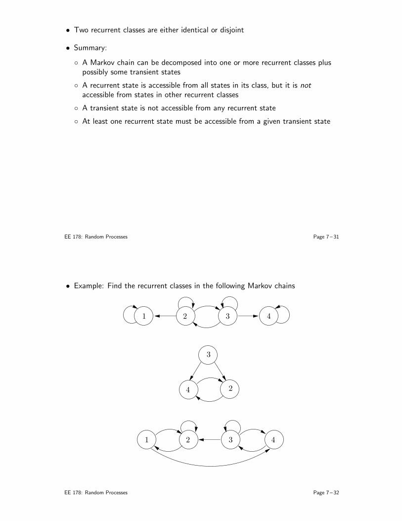
• Two recurrent classes are either identical or disjoint
• Summary:
A Markov chain can be decomposed into one or more recurrent classes pluspossibly some transient states
A recurrent state is accessible from all states in its class, but it is notaccessible from states in other recurrent classes
A transient state is not accessible from any recurrent state
At least one recurrent state must be accessible from a given transient state
EE 178: Random Processes Page 7 – 31
• Example: Find the recurrent classes in the following Markov chains
1 2
2
2
3
3
3
4
4
41
EE 178: Random Processes Page 7 – 32
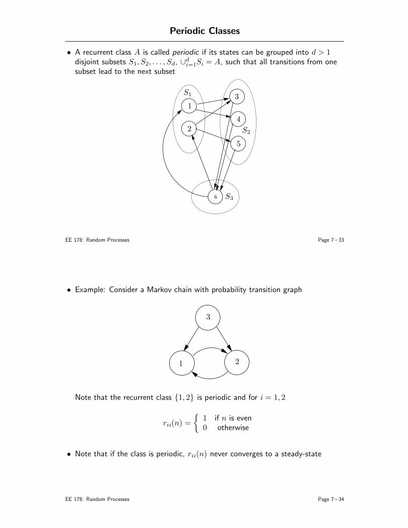
Periodic Classes
• A recurrent class A is called periodic if its states can be grouped into d > 1disjoint subsets S1, S2, . . . , Sd, ∪
di=1Si = A, such that all transitions from one
subset lead to the next subset
6
1
2
3
4
5
S1
S2
S3
EE 178: Random Processes Page 7 – 33
• Example: Consider a Markov chain with probability transition graph
2
3
1
Note that the recurrent class 1, 2 is periodic and for i = 1, 2
rii(n) =
1 if n is even0 otherwise
• Note that if the class is periodic, rii(n) never converges to a steady-state
EE 178: Random Processes Page 7 – 34
Steady State Probabilities
• Steady-state convergence theorem: If a Markov chain has only one recurrentclass and it is not periodic, then rij(n) tends to a steady-state πj independent
of i, i.e.,lim
n→∞
rij(n) = πj for all i
• Steady-state equations: Taking the limit as n → ∞ of theChapman-Kolmogorov equations
rij(n+ 1) =m∑
k=1
rik(n)pkj for 1 ≤ i, j ≤ m,
we obtain the set of linear equations, called the balance equations:
πj =m∑
k=1
πkpkj for j = 1, 2, . . . ,m
The balance equations together with the normalization equation
m∑
j=1
πj = 1,
EE 178: Random Processes Page 7 – 35
uniquely determine the steady state probabilities π1, π2, . . . , πm
• The balance equations can be expressed in a matrix form as:
ΠP = Π, where Π = [π1 π2 . . . , πm]
• In general there are m− 1 linearly independent balance equations
• The steady state probabilities form a probability distribution over the statespace, called the stationary distribution of the chain. If we set PX0 = j = πj
for j = 1, 2, . . . ,m, we have PXn = j = πj for all n ≥ 1 and j = 1, 2, . . . ,m
• Example: Binary Symmetric Markov Chain
P =
[
1− p pp 1− p
]
Find the steady-state probabilities
Solution: We need to solve the balance and normalization equations
π1 = p11π1 + p21π2 = (1− p)π1 + pπ2
π2 = p12π1 + p22π2 = pπ1 + (1− p)π2
1 = π1 + π2
EE 178: Random Processes Page 7 – 36
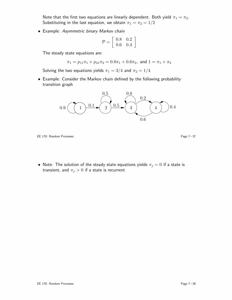
Note that the first two equations are linearly dependent. Both yield π1 = π2.Substituting in the last equation, we obtain π1 = π2 = 1/2
• Example: Asymmetric binary Markov chain
P =
[
0.8 0.20.6 0.4
]
The steady state equations are:
π1 = p11π1 + p21π2 = 0.8π1 + 0.6π2, and 1 = π1 + π2
Solving the two equations yields π1 = 3/4 and π2 = 1/4
• Example: Consider the Markov chain defined by the following probabilitytransition graph
1 2 3 40.90.1
0.5
0.5
0.80.2
0.6
0.4
EE 178: Random Processes Page 7 – 37
• Note: The solution of the steady state equations yields πj = 0 if a state istransient, and πj > 0 if a state is recurrent
EE 178: Random Processes Page 7 – 38
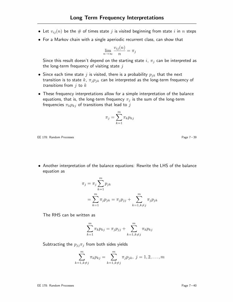
Long Term Frequency Interpretations
• Let vij(n) be the # of times state j is visited beginning from state i in n steps
• For a Markov chain with a single aperiodic recurrent class, can show that
limn→∞
vij(n)
n= πj
Since this result doesn’t depend on the starting state i, πj can be interpreted asthe long-term frequency of visiting state j
• Since each time state j is visited, there is a probability pjk that the nexttransition is to state k, πjpjk can be interpreted as the long-term frequency oftransitions from j to k
• These frequency interpretations allow for a simple interpretation of the balanceequations, that is, the long-term frequency πj is the sum of the long-termfrequencies πkpkj of transitions that lead to j
πj =m∑
k=1
πkpkj
EE 178: Random Processes Page 7 – 39
• Another interpretation of the balance equations: Rewrite the LHS of the balanceequation as
πj = πj
m∑
k=1
pjk
=m∑
k=1
πjpjk = πjpjj +m∑
k=1,k 6=j
πjpjk
The RHS can be written as
m∑
k=1
πkpkj = πjpjj +m∑
k=1,k 6=j
πkpkj
Subtracting the pjjπj from both sides yields
m∑
k=1,k 6=j
πkpkj =m∑
k=1,k 6=j
πjpjk, j = 1, 2, . . . ,m
EE 178: Random Processes Page 7 – 40
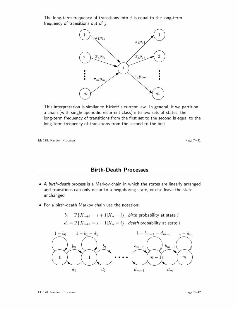
The long-term frequency of transitions into j is equal to the long-termfrequency of transitions out of j
j
1 1
2 2
mm
π1p1j
π2p2j
πmpmj
πjpj1
πjpj2
πjpjm
This interpretation is similar to Kirkoff’s current law. In general, if we partitiona chain (with single aperiodic recurrent class) into two sets of states, thelong-term frequency of transitions from the first set to the second is equal to thelong-term frequency of transitions from the second to the first
EE 178: Random Processes Page 7 – 41
Birth-Death Processes
• A birth-death process is a Markov chain in which the states are linearly arrangedand transitions can only occur to a neighboring state, or else leave the stateunchanged
• For a birth-death Markov chain use the notation:
bi = PXn+1 = i+ 1|Xn = i, birth probability at state i
di = PXn+1 = i− 1|Xn = i, death probability at state i
0 1 m− 1 m
1− b0
b0
1− b1 − d1
b1
d1 d2 dm−1 dm
bm−2 bm−1
1− bm−1 − dm−1 1− dm
EE 178: Random Processes Page 7 – 42
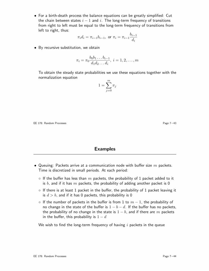
• For a birth-death process the balance equations can be greatly simplified: Cutthe chain between states i− 1 and i. The long-term frequency of transitionsfrom right to left must be equal to the long-term frequency of transitions fromleft to right, thus:
πidi = πi−1bi−1, or πi = πi−1bi−1
di
• By recursive substitution, we obtain
πi = π0b0b1 . . . bi−1
d1d2 . . . di, i = 1, 2, . . . ,m
To obtain the steady state probabilities we use these equations together with thenormalization equation
1 =m∑
j=0
πj
EE 178: Random Processes Page 7 – 43
Examples
• Queuing: Packets arrive at a communication node with buffer size m packets.Time is discretized in small periods. At each period:
If the buffer has less than m packets, the probability of 1 packet added to itis b, and if it has m packets, the probability of adding another packet is 0
If there is at least 1 packet in the buffer, the probability of 1 packet leaving itis d > b, and if it has 0 packets, this probability is 0
If the number of packets in the buffer is from 1 to m− 1, the probability ofno change in the state of the buffer is 1− b− d. If the buffer has no packets,the probability of no change in the state is 1− b, and if there are m packetsin the buffer, this probability is 1− d
We wish to find the long-term frequency of having i packets in the queue
EE 178: Random Processes Page 7 – 44
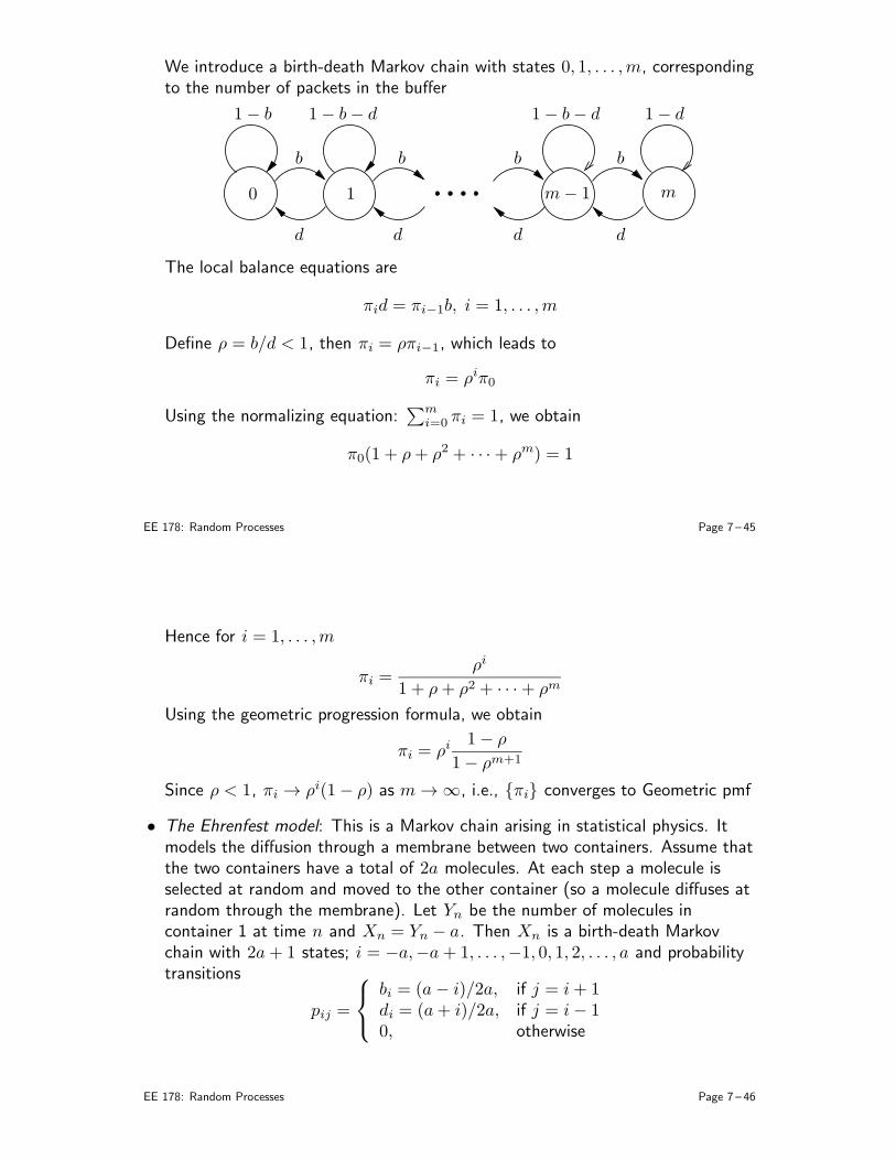
We introduce a birth-death Markov chain with states 0, 1, . . . ,m, correspondingto the number of packets in the buffer
0 1 m− 1 m
1− b
b
1− b− d
b
d d d d
b b
1− b− d 1− d
The local balance equations are
πid = πi−1b, i = 1, . . . ,m
Define ρ = b/d < 1, then πi = ρπi−1, which leads to
πi = ρiπ0
Using the normalizing equation:∑m
i=0 πi = 1, we obtain
π0(1 + ρ+ ρ2 + · · ·+ ρm) = 1
EE 178: Random Processes Page 7 – 45
Hence for i = 1, . . . ,m
πi =ρi
1 + ρ+ ρ2 + · · ·+ ρm
Using the geometric progression formula, we obtain
πi = ρi1− ρ
1− ρm+1
Since ρ < 1, πi → ρi(1− ρ) as m → ∞, i.e., πi converges to Geometric pmf
• The Ehrenfest model: This is a Markov chain arising in statistical physics. Itmodels the diffusion through a membrane between two containers. Assume thatthe two containers have a total of 2a molecules. At each step a molecule isselected at random and moved to the other container (so a molecule diffuses atrandom through the membrane). Let Yn be the number of molecules incontainer 1 at time n and Xn = Yn − a. Then Xn is a birth-death Markovchain with 2a+ 1 states; i = −a,−a+ 1, . . . ,−1, 0, 1, 2, . . . , a and probabilitytransitions
pij =
bi = (a− i)/2a, if j = i+ 1di = (a+ i)/2a, if j = i− 10, otherwise
EE 178: Random Processes Page 7 – 46
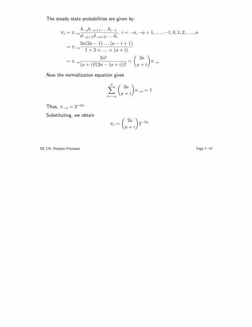
The steady state probabilities are given by:
πi = π−ab−ab−a+1 . . . bi−1
d−a+1d−a+2 . . . di, i = −a,−a+ 1, . . . ,−1, 0, 1, 2, . . . , a
= π−a2a(2a− 1) . . . (a− i+ 1)
1× 2× . . .× (a+ i)
= π−a2a!
(a+ i)!(2a− (a+ i))!=
(
2a
a+ i
)
π−a
Now the normalization equation gives
a∑
i=−a
(
2a
a+ i
)
π−a = 1
Thus, π−a = 2−2a
Substituting, we obtain
πi =
(
2a
a+ i
)
2−2a
EE 178: Random Processes Page 7 – 47