Economic Analysis Papers

The Gender Wage Gap in Cyprus

Louis N. Christofides Kostantinos Vrachimis

Department of Economics and Economics Research Centre

University of Cyprus

No. 10-07

December 2007

Publication Editors: Costas Hadjiyiannis, Theodoros Zachariadis

ERC Sponsors (in alphabetical order)

Association of Cyprus Commercial Banks

Central Bank of Cyprus

Cyprus Tourism Organisation

Economics Department, University of Cyprus

Ministry of Finance

Ministry of Labour and Social Security

Planning Bureau

University of Cyprus

Disclaimer: the views expressed in the Economic Policy Papers and Economic Analysis Papers are of the authors and do not necessarily represent the ERC.

ii

The Gender Wage Gap in Cyprus

Louis N. Christofides and Kostantinos Vrachimis

Abstract

The objective of this study is to examine the gender wage gap in Cyprus over time, using available data from the Cyprus Surveys of Household Expenditure and Income of 1990/91, 1996/97 and 2002/03. The results show that the observed wage gap declined from 0.572 ln wage points in 1990/91 to 0.313 points in 1996/97 and to 0.26 points in 2002/03. The large reduction by 1996/97 was, in part, due to an improvement in the productivity characteristics (specifically education) of female employees. However, by the 1996/97 Survey, no scope for significant further reductions in the gap due to improved characteristics was possible, leaving the observed gap of 0.313 ln wage points unexplained and due either to unobserved characteristics or discrimination. This also holds for the observed gap of 0.26 points in 2002/03. Quantile regressions which focus on the wage gap at different points of the ln wage distribution reveal that, despite the considerable progress achieved by women in moving through the ranks of the distribution, the pay gap is largest at the highest levels of the ln wage distribution in all three Surveys.

iii

iv

v

CONTENTS

ΠΕΡΙΛΗΨΗ ............................................................................................................................................... VII

I. INTRODUCTION.......................................................................................................................................1

II. INSTITUTIONAL BACKGROUND...........................................................................................................2

III. DATA DESCRIPTION AND ECONOMETRIC MODEL ..........................................................................5

IV. WAGE DECOMPOSITIONS.................................................................................................................13

V. THE DISTRIBUTION OF THE WAGE GAP ..........................................................................................16

VI. CONCLUSIONS ...................................................................................................................................18

REFERENCES...........................................................................................................................................19

APPENDIX A: VARIABLE DESCRIPTION ...............................................................................................20

APPENDIX B: AUXILIARY ESTIMATION RESULTS ...............................................................................21

vi

vii

ΠΕΡΙΛΗΨΗ

Ο σκοπός αυτής της έρευνας είναι να εξετάσει διαχρονικά το μισθολογικό χάσμα μεταξύ των δυο φύλων στην Κύπρο. Τα στοιχεία που χρησιμοποιούνται προέρχονται από τις Έρευνες Οικογενειακών Προϋπολογισμών για τα έτη 1990/91, 1996/97 και 2002/03. Τα αποτελέσματα της έρευνας δείχνουν ότι το μέσο μισθολογικό χάσμα μειώθηκε από 0.572 λογαριθμικές μονάδες το 1990/91 στις 0.313 μονάδες το 1996/97 και στις 0.26 μονάδες το 2002/03. Αυτή η μείωση οφείλεται στη βελτίωση των παραγωγικών χαρακτηριστικών (π.χ. μόρφωση) του γυναικείου εργατικού δυναμικού. Όμως, το χάσμα του 1996/97 και του 2002/03 δεν μπορεί να εξηγηθεί από εναπομένουσες διαφορές στα παραγωγικά χαρακτηριστικά των δύο φύλων και οφείλεται μάλλον σε διαφορές σε μη μετρήσιμα χαρακτηριστικά ή και σε πιθανές διακρίσεις. Επιπλέον η ανάλυση της κατανομής του χάσματος δείχνει ότι, σε όλες τις Έρευνες, η μεγαλύτερη διαφορά εναντίον των γυναικών συμβαίνει στις υψηλά αμειβόμενες υπαλλήλους.

viii

1

I. INTRODUCTION

A significant issue that has drawn a lot of attention is the observed difference between the compensation received by employees of different genders. Many studies indicate that female employees receive lower wages compared to their male counterparts. In theory, wages are connected to productivity and, in a non-discriminatory environment, differences in wages should simply reflect productivity. Productivity cannot be measured directly, so measurable characteristics, such as experience and education, are used as proxies. Armed with these proxies, analysts divide the unconditional gender wage gap in two parts, one attributed to observable characteristics, which may to an extent account for the unconditional gap, and a second part which is unexplained and may be due to a combination of omitted unmeasurable characteristics (e.g. the likelihood that a woman will reduce her commitment to the labour market in order to raise her family) and discrimination.

The gender gap has drawn considerable attention from national and international governments (e.g. the European Union) and organizations such as the International Labour Organization (ILO). National legislation has been passed that forbids discrimination against women, creating monitoring bodies that enforce these legislations. In Cyprus, harmonization with the Acquis Communautaire has led to the passing of several new pieces of legislation. Another fact that highlighted attention to this problem is that, despite the progress that has been made during the last decades, Cyprus has consistently compared unfavourably to other European Union countries concerning the extent of the gender pay gap.

This study uses data from Cyprus Surveys of Household Expenditure and Income (CSHEI), and examines the evolution of the pay gap and its determinants. This analysis is performed using a variant of decompositions proposed by Neumark (1988) and Oaxaca and Ransom (1994). In addition, quantile regression methodology is used to determine the distribution of the wage gap across earnings classes and over time.

The organization of the study is as follows: Section II provides background information, section III describes the data and the econometric model used, section IV presents the wage decompositions, section V the quantile regression results and section VI summarises the findings of the study.

2

II. INSTITUTIONAL BACKGROUND

A previous study by Christofides and Pashardes (2000) indicated that, in 1991, the unconditional average female weekly wage, as recorded in the CSHEI database for 1990/91, was sixty percent of the male wage. Their study also showed that forty percent of the wage gap cannot be explained by the differences in the observed productivity characteristics of the two genders. In addition a large part of the explained part is attributed to industry effects. The study by Panayiotou (2006), commissioned by the European Union, evaluated the gender wage gap in Cyprus from a policy perspective. As indicated by Panayiotou (2006), the gender pay gap is sometimes attributed to the absence of strong laws against discrimination, a low employment rate for women, lower educational attainment for women, a high rate of part-time employment by women, or a large gap in the average number of hours worked between men and women. These factors do not, in general, apply for Cyprus. The author speculates that the gender wage gap may be due to the fact that female workers tend to be concentrated in a small number of poorly paid occupations (Cyprus has the highest gender segregation among new EU countries), mainly in the service sector. In addition, most of the professions that women choose to enter do not offer opportunities for career advancement, an effect known as a “sticky floor”. Also, women have difficulty capturing highly paid positions, such as manager or director, an effect known as the “glass ceiling”. This is reflected in part in data published by the Cyprus Statistical Service that shows that, in 2006, only sixteen percent of the decision-making posts in the labour force (administrative and managerial personnel) were held by women. In 2007 and 2005 respectively, thirty-six percent of judges and twenty-three percent of senior level civil servants were women. In 2006 only fourteen percent of the Members of the House of Representatives were women. Finally, in 2007, twenty percent of the members of Municipal or other local area governing bodies are women.

Cyprus governments have introduced several pieces of legislation, in line with EU guidelines, aiming for the equal pay treatment of the genders. Additional legislation regulates other rights, like maternity leave. There are two major laws that deal with the equality of the two genders in the workspace. The first one is the Equal Pay Between Men and Women for the Same Work or for Work of Equal Value Law, 2002,2004 (L.177(I)/2002,L.193(I)/2004) and its amendments of 2004 and 2007 (L.58(I)2004 and L.50(I)/2007). The second one is the Equal Treatment of Men and Women in Employment and Vocational Training Law, 2002 (L.205(I)/2002) and its amendment Equal Treatment of Men and Women in Employment and Vocational Training Law (Amendment), 2006 (L45(I)/2006). The first law requires that men and women receive the same compensation for equal work or for work of equal value. The aim of the second law is to ensure that all workers have an equal right to employment, access to

3

education and are treated in the same way on dismissal. Also, through legislation, monitoring bodies are created that can take action against the violation of the legislation by employers. Another Law, the Equal Treatment of Men and Women in Professional Social Insurance Schemes Law, 2002 (L. 133(I)/2002), has as its main objective to ensure that men and women are equally treated in occupational social security schemes. In addition, the Government of Cyprus has ratified international conventions aiming at the elimination of the gender wage gap, such as the ILO Equal Remunerator Convention (No.100/1951), ratified in 1987.

Another string of legislation deals with parental leave. The Maternity Protection Law, 1997 (L. 100(I)/1997) and its amendments (the Maternity Protection (Amendment) Law, 2000 and 2002 (L. 45(I)/2000 and L. 64(I)/2002), entitles female employees with sixteen weeks of paid leave, to receive seventy-five percent of their monthly wage throughout this period. Recent changes increase this leave to eighteen weeks. Another law, the Parental Leave and Leave on Grounds of Force Majeure Law, 2002, (L. 69(I)/2002), entitles both parents to unpaid leave of up to thirteen weeks. In addition, under extreme and urgent family circumstances both parents are entitled to up to seven days of unpaid leave each year.

Another state policy that affects professions that are mainly occupied by female employees is the minimum wage legislation. An order, made each June by the Council of Ministers, sets the minimum wage for the whole year. This order is specifically aimed at low-paid workers, such as day care workers, clerks, nurses, and shop and office assistants. The minimum monthly wage set for 2007 is 434 pounds. The goal that has been set by the Government is to gradually raise the minimum wage to fifty percent of the national average wage. Since 1995 the minimum wage has fluctuated around forty-two percent of the national mean wage.

It must also be noticed that in Cyprus the childcare system is inadequate. There is no public scheme covering children until the age of five. This gap is filled by private schools at considerable economic cost to households. The number of available places is limited and the schedules, in most cases, are inflexible. However, compulsory schooling starts at the age of five and is free for each child.

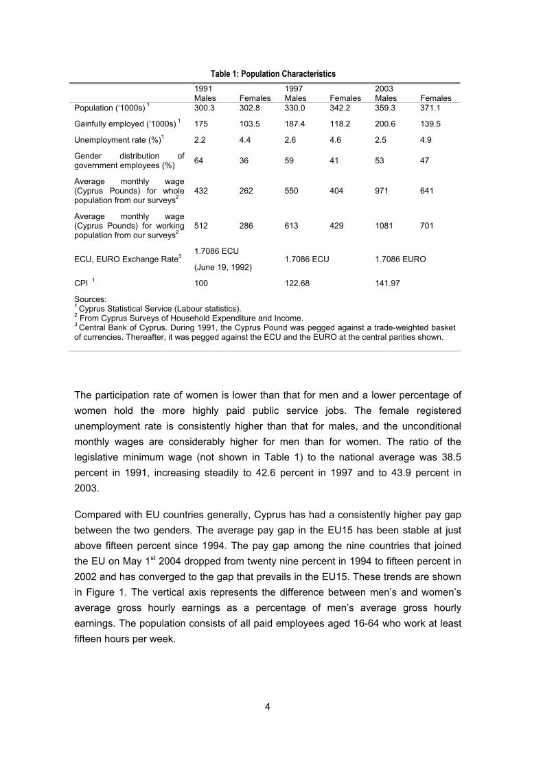
Table 1 provides some basic statistics on labour market involvement and outcomes by gender.

4

Table 1: Population Characteristics 1991 1997 2003 Males Females Males Females Males Females Population (‘1000s) 1 300.3 302.8 330.0 342.2 359.3 371.1

Gainfully employed (‘1000s) 1 175 103.5 187.4 118.2 200.6 139.5

Unemployment rate (%)1 2.2 4.4 2.6 4.6 2.5 4.9

Gender distribution of government employees (%) 64 36 59 41 53 47

Average monthly wage (Cyprus Pounds) for whole population from our surveys2

432 262 550 404 971 641

Average monthly wage (Cyprus Pounds) for working population from our surveys2

512 286 613 429 1081 701

ECU, EURO Exchange Rate3 1.7086 ECU

(June 19, 1992) 1.7086 ECU 1.7086 EURO

CPI 1 100 122.68 141.97

Sources: 1 Cyprus Statistical Service (Labour statistics). 2 From Cyprus Surveys of Household Expenditure and Income. 3 Central Bank of Cyprus. During 1991, the Cyprus Pound was pegged against a trade-weighted basket of currencies. Thereafter, it was pegged against the ECU and the EURO at the central parities shown.

The participation rate of women is lower than that for men and a lower percentage of women hold the more highly paid public service jobs. The female registered unemployment rate is consistently higher than that for males, and the unconditional monthly wages are considerably higher for men than for women. The ratio of the legislative minimum wage (not shown in Table 1) to the national average was 38.5 percent in 1991, increasing steadily to 42.6 percent in 1997 and to 43.9 percent in 2003.

Compared with EU countries generally, Cyprus has had a consistently higher pay gap between the two genders. The average pay gap in the EU15 has been stable at just above fifteen percent since 1994. The pay gap among the nine countries that joined the EU on May 1st 2004 dropped from twenty nine percent in 1994 to fifteen percent in 2002 and has converged to the gap that prevails in the EU15. These trends are shown in Figure 1. The vertical axis represents the difference between men’s and women’s average gross hourly earnings as a percentage of men’s average gross hourly earnings. The population consists of all paid employees aged 16-64 who work at least fifteen hours per week.

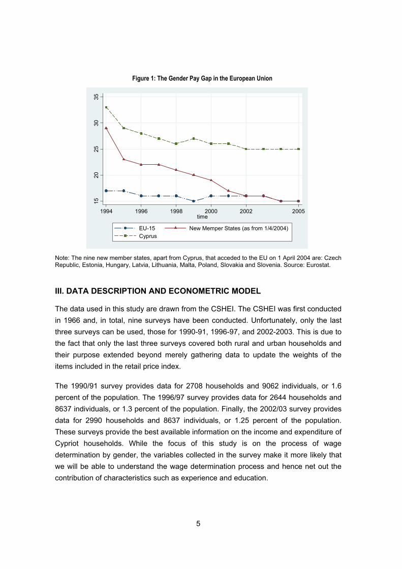
Figure 1: The Gender Pay Gap in the European Union

1520

2530

35

1994 1996 1998 2000 2002 2005time

EU-15 New Memper States (as from 1/4/2004)Cyprus

Note: The nine new member states, apart from Cyprus, that acceded to the EU on 1 April 2004 are: Czech Republic, Estonia, Hungary, Latvia, Lithuania, Malta, Poland, Slovakia and Slovenia. Source: Eurostat.

III. DATA DESCRIPTION AND ECONOMETRIC MODEL

The data used in this study are drawn from the CSHEI. The CSHEI was first conducted in 1966 and, in total, nine surveys have been conducted. Unfortunately, only the last three surveys can be used, those for 1990-91, 1996-97, and 2002-2003. This is due to the fact that only the last three surveys covered both rural and urban households and their purpose extended beyond merely gathering data to update the weights of the items included in the retail price index.

The 1990/91 survey provides data for 2708 households and 9062 individuals, or 1.6 percent of the population. The 1996/97 survey provides data for 2644 households and 8637 individuals, or 1.3 percent of the population. Finally, the 2002/03 survey provides data for 2990 households and 8637 individuals, or 1.25 percent of the population. These surveys provide the best available information on the income and expenditure of Cypriot households. While the focus of this study is on the process of wage determination by gender, the variables collected in the survey make it more likely that we will be able to understand the wage determination process and hence net out the contribution of characteristics such as experience and education.

5

6

The ‘working’ sample consists of data for 5187, 5761 and 6474 individuals from the three surveys respectively. We include in the sample only individuals aged sixteen to seventy-five, who have declared their education level and for whom other reliable data are available. This is because we include only individuals who are allowed to work (individuals aged sixteen and above) and we exclude individuals who are not capable of working. Also, we include in our sample only households containing first degree relatives, i.e. the head of the household, his/her partner and their children. The aim of this restriction is to more accurately assign family income, which is only available at the household level, to each member of the household. Thus, family income from financial assets, which may affect the behaviour of the individuals studied, should be truly their income and not that of other members of the family or even of unrelated individuals. Also, through this restriction, we exclude certain individuals like housekeepers or non-relatives who live in the household. The ‘selected’ sub-sample of the working sample consists of those individuals who had paid employment and a non-zero wage. The reason for selecting this group is that the self-employed are prone to under-report their earnings and, in any case, the wage determination process is rather different for them. Given these restrictions our sample consists of 1405 men and 1013 women from the 1990/91 survey, 1534 men and 1038 women from the 1996/97 survey, and 1683 men and 1379 women from the 2002/03 survey.

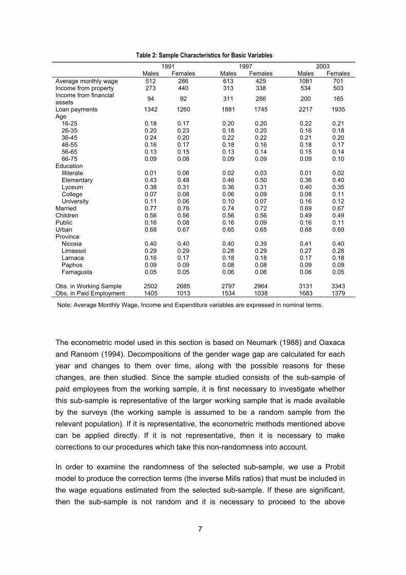
The surveys report a wealth of information about the personal characteristics of each individual. These characteristics include age, education, place of residence, number of children and marital status. Also, they include information about working status, whether the individual was working in the public sector, the industry of employment and his or her occupation. In addition, information on income and expenditure sources is available. As can be seen from Table 2, the difference in the mean value of the nominal1 wage rate for men and women in 1991 was 226 CYP per month and dropped substantially to 184 CYP per month in 1997 but increased to 380 CYP per month in 2003. Table 2 also indicates noteworthy differences in the average characteristics of the two genders in all surveys. For instance, the proportion of women in the working sample who have college or university education increases from 0.14 in 1991 to 0.23 in 2003 and became roughly equal to that for men in the last two surveys.

1 The variables used throughout the study are in nominal terms. If the study were carried out using real terms the estimation results would not change apart from a change in the value of the constant term. The decomposition results regarding important characteristics would not be affected.

7

Table 2: Sample Characteristics for Basic Variables 1991 1997 2003 Males Females Males Females Males Females Average monthly wage 512 286 613 429 1081 701 Income from property 273 440 313 338 534 503 Income from financial assets 94 92 311 286 200 165

Loan payments 1342 1260 1881 1745 2217 1935 Age

16-25 0.18 0.17 0.20 0.20 0.22 0.21 26-35 0.20 0.23 0.18 0.20 0.16 0.18 36-45 0.24 0.20 0.22 0.22 0.21 0.20 46-55 0.16 0.17 0.18 0.16 0.18 0.17 56-65 0.13 0.15 0.13 0.14 0.15 0.14 66-75 0.09 0.08 0.09 0.09 0.09 0.10

Education Illiterate 0.01 0.06 0.02 0.03 0.01 0.02 Elementary 0.43 0.48 0.46 0.50 0.36 0.40 Lyceum 0.38 0.31 0.36 0.31 0.40 0.35 College 0.07 0.08 0.06 0.09 0.08 0.11 University 0.11 0.06 0.10 0.07 0.16 0.12

Married 0.77 0.76 0.74 0.72 0.69 0.67 Children 0.56 0.56 0.56 0.56 0.49 0.49 Public 0.16 0.08 0.16 0.09 0.16 0.11 Urban 0.68 0.67 0.65 0.65 0.68 0.69 Province

Nicosia 0.40 0.40 0.40 0.39 0.41 0.40 Limassol 0.29 0.29 0.28 0.29 0.27 0.28 Larnaca 0.16 0.17 0.18 0.18 0.17 0.18 Paphos 0.09 0.09 0.08 0.08 0.09 0.09 Famagusta 0.05 0.05 0.06 0.06 0.06 0.05

Obs. in Working Sample 2502 2685 2797 2964 3131 3343 Obs. in Paid Employment 1405 1013 1534 1038 1683 1379

Note: Average Monthly Wage, Income and Expenditure variables are expressed in nominal terms.

The econometric model used in this section is based on Neumark (1988) and Oaxaca and Ransom (1994). Decompositions of the gender wage gap are calculated for each year and changes to them over time, along with the possible reasons for these changes, are then studied. Since the sample studied consists of the sub-sample of paid employees from the working sample, it is first necessary to investigate whether this sub-sample is representative of the larger working sample that is made available by the surveys (the working sample is assumed to be a random sample from the relevant population). If it is representative, the econometric methods mentioned above can be applied directly. If it is not representative, then it is necessary to make corrections to our procedures which take this non-randomness into account.

In order to examine the randomness of the selected sub-sample, we use a Probit model to produce the correction terms (the inverse Mills ratios) that must be included in the wage equations estimated from the selected sub-sample. If these are significant, then the sub-sample is not random and it is necessary to proceed to the above

decompositions taking these terms into account. On the other hand, if the inverse Mills ratios are not significant, then the selected sub-sample may be treated as random and it is possible to analyze it without taking the inverse Mills ratios into account.

An alternative procedure is to estimate the two-equation system (selection into the sub-sample using a Probit mechanism and the wage equation of the sub-sample) using a maximum likelihood method that considers whether the selection from the working sample into the selected sub-sample is conditioned by a correlation between the random error terms in the selection and the wage equation. If a positive (say) correlation exists, then those who (due to unobserved error terms) are more likely to be paid employees (and be selected into the sub-sample) are also more likely to be high wage earners and the sub-sample will produce biased estimates if this process is not taken into account. If a non-zero correlation between the error terms exists, the maximum likelihood estimation procedure will take this into account and produce unbiased estimates. If the correlation coefficient is not significantly different from zero, then the two equations may be estimated separately and there is no selection issue.

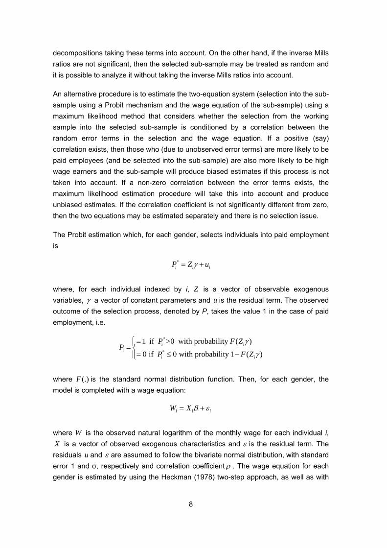
The Probit estimation which, for each gender, selects individuals into paid employment is

8

*ii iP Z uγ= +

Zwhere, for each individual indexed by i, is a vector of observable exogenous variables, γ a vector of constant parameters and u is the residual term. The observed outcome of the selection process, denoted by P, takes the value 1 in the case of paid employment, i.e.

*

*

1 if >0 with probability ( )

0 if 0 with probability 1 ( )i i

ii i

P FP

P F

γZ

Z γ

⎧=⎪= ⎨= ≤ −⎪⎩

where is the standard normal distribution function. Then, for each gender, the model is completed with a wage equation:

(.)F

i iW X iβ ε= +

where W is the observed natural logarithm of the monthly wage for each individual i, X is a vector of observed exogenous characteristics and ε is the residual term. The residuals u and ε are assumed to follow the bivariate normal distribution, with standard error 1 and σ, respectively and correlation coefficient ρ . The wage equation for each gender is estimated by using the Heckman (1978) two-step approach, as well as with

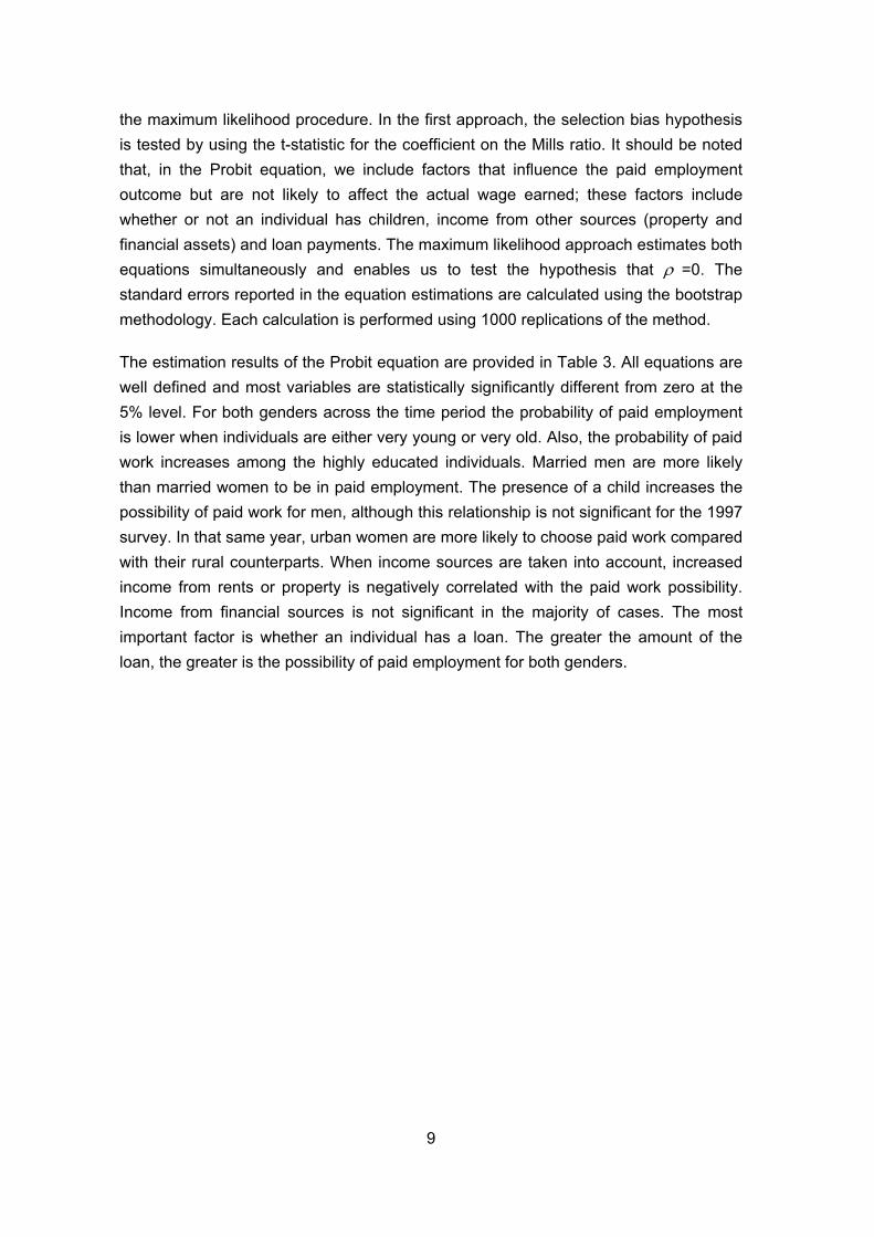
the maximum likelihood procedure. In the first approach, the selection bias hypothesis is tested by using the t-statistic for the coefficient on the Mills ratio. It should be noted that, in the Probit equation, we include factors that influence the paid employment outcome but are not likely to affect the actual wage earned; these factors include whether or not an individual has children, income from other sources (property and financial assets) and loan payments. The maximum likelihood approach estimates both equations simultaneously and enables us to test the hypothesis that ρ =0. The standard errors reported in the equation estimations are calculated using the bootstrap methodology. Each calculation is performed using 1000 replications of the method.

The estimation results of the Probit equation are provided in Table 3. All equations are well defined and most variables are statistically significantly different from zero at the 5% level. For both genders across the time period the probability of paid employment is lower when individuals are either very young or very old. Also, the probability of paid work increases among the highly educated individuals. Married men are more likely than married women to be in paid employment. The presence of a child increases the possibility of paid work for men, although this relationship is not significant for the 1997 survey. In that same year, urban women are more likely to choose paid work compared with their rural counterparts. When income sources are taken into account, increased income from rents or property is negatively correlated with the paid work possibility. Income from financial sources is not significant in the majority of cases. The most important factor is whether an individual has a loan. The greater the amount of the loan, the greater is the possibility of paid employment for both genders.

9

10

Table 3: Probit Choice of Paid Employment 1991 1997 2003

Males Females Males Females Males Females Age

16-25 -0.476*** -0.369*** -0.455*** -0.392*** -0.778*** -0.766*** (0.132) (0.097) (0.116) (0.097) (0.108) (0.103) 26-35 0.114 -0.067 0.161* -0.090 0.162* 0.105 (0.092) (0.078) (0.088) (0.074) (0.093) (0.076) 46-55 0.021 -0.066 0.059 -0.183** -0.225*** -0.123* (0.092) (0.088) (0.082) (0.085) (0.082) (0.073) 56-65 -0.486*** -0.835*** -0.559*** -0.595*** -0.710*** -0.897*** (0.104) (0.114) (0.095) (0.110) (0.089) (0.090) 66-75 -1.726*** -1.761*** -1.483*** -1.854*** -1.776*** -2.223***

(0.151) (0.213) (0.126) (0.236) (0.130) (0.219) Education

Illiterate -0.163 0.242 0.043 -0.015 -0.685** -0.776*** (0.287) (0.163) (0.226) (0.231) (0.343) (0.291) Lyceum 0.449*** 0.419*** 0.368*** 0.438*** 0.349*** 0.386*** (0.069) (0.068) (0.060) (0.062) (0.057) (0.061) College 0.731*** 0.874*** 0.673*** 0.825*** 0.600*** 0.739*** (0.124) (0.108) (0.126) (0.098) (0.101) (0.084) University 0.535*** 0.819*** 0.451*** 0.960*** 0.610*** 0.845*** (0.108) (0.118) (0.100) (0.108) (0.083) (0.091)

Married 0.429*** -0.468*** 0.742*** -0.025 0.406*** 0.089 (0.129) (0.084) (0.115) (0.084) (0.096) (0.073) Children 0.219** 0.068 0.004 0.145* 0.185** 0.093 (0.086) (0.076) (0.081) (0.079) (0.075) (0.068) Income from property -0.019 -0.041*** -0.021** -0.028*** -0.007 -0.034*** (0.012) (0.011) (0.011) (0.011) (0.009) (0.009) Income from financial assets

-0.048*** 0.014 0.017 -0.007 -0.020* -0.014

(0.013) (0.012) (0.010) (0.010) (0.010) (0.012) Loan payments 0.028*** 0.021*** 0.018** 0.031*** 0.005 0.037*** (0.008) (0.008) (0.008) (0.008) (0.008) (0.008) Urban 0.052 0.103 -0.021 0.210*** -0.033 0.119** (0.067) (0.066) (0.061) (0.058) (0.059) (0.060) Province

Nicosia -0.099 0.254*** -0.018 0.246*** 0.113* 0.201*** (0.069) (0.065) (0.064) (0.064) (0.063) (0.059) Paphos -0.162 -0.203* -0.276*** -0.027 -0.047 0.104 (0.112) (0.110) (0.106) (0.109) (0.095) (0.093) Larnaca -0.080 -0.090 -0.077 0.127 -0.004 -0.007 (0.092) (0.082) (0.082) (0.081) (0.076) (0.076) Famagusta -0.191 -0.077 -0.367*** 0.323** -0.081 0.142 (0.144) (0.145) (0.138) (0.132) (0.137) (0.129)

Constant -0.243* -0.164 -0.353*** -0.766*** -0.102 -0.447*** (0.145) (0.112) (0.126) (0.112) (0.118) (0.109) Observations 2502 2685 2797 2964 3131 3343 Chi-square (27) 554.24 363.45 542.87 425.99 770.96 735.29

Significance at the 1%, 5%, 10% level is denoted by ***/**/* respectively. Standard errors in parentheses. Description of the variables and list of excluded categories are provided in Appendix A.

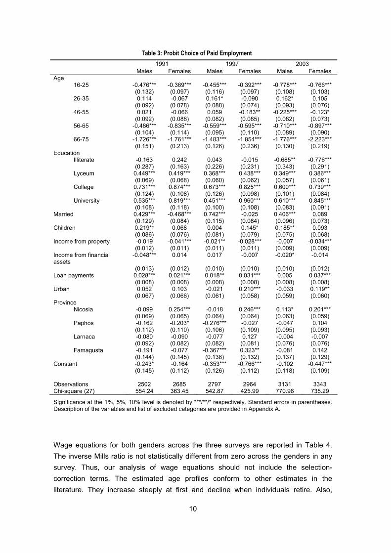
Wage equations for both genders across the three surveys are reported in Table 4. The inverse Mills ratio is not statistically different from zero across the genders in any survey. Thus, our analysis of wage equations should not include the selection-correction terms. The estimated age profiles conform to other estimates in the literature. They increase steeply at first and decline when individuals retire. Also,

11

wages increase with education. Married individuals do not get a higher wage in most cases. Two important factors that influence wage determination are the area in which an individual lives and whether the individual works in the public sector. Urban individuals across genders receive higher wages than rural residents. This effect increased from 1991 to 1997, but decreased in 2003. Public sector employees always receive a larger wage. In the last two surveys, the difference between female public sector employees and female private sector employees is smaller compared with the differences for their male counterparts. The coefficients for the industry effects are quite reasonable and indicate that, in comparison to the omitted category (being public sector employees, education and health), individuals across genders who work in agriculture, fishing construction and manufacture are less well paid. Men working in construction are becoming better paid, a fact that is associated with a recent construction and real-estate industry boom in Cyprus. This can also be seen in the coefficient in the business services industry dummy for the male population in 2003. The industry effect for financial services is significantly positive across genders and all years.

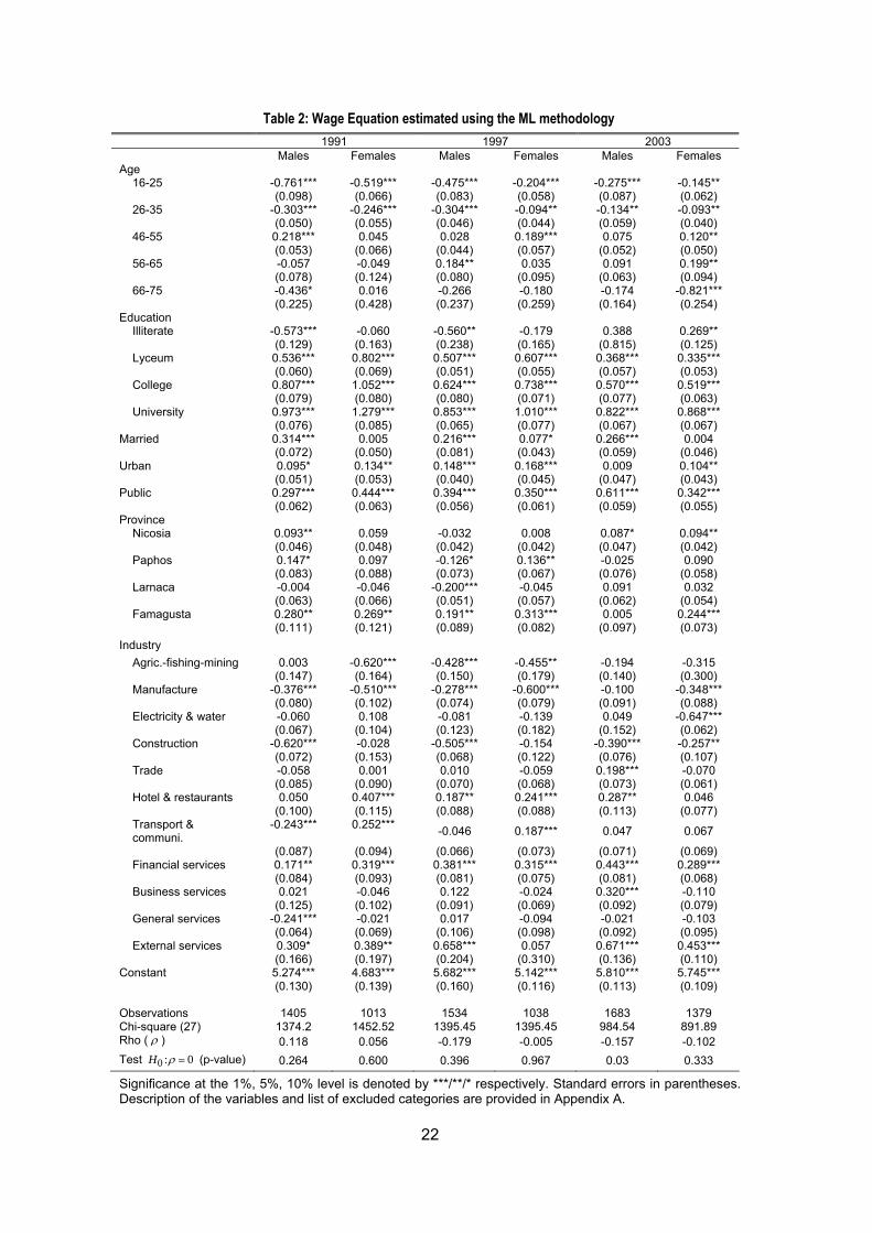
In Appendix B, Table 2, results obtained based on the Maximum Likelihood approach are presented. The results obtained are very similar to those presented in the previous paragraphs. In particular, the hypothesis that the error terms in the two equations are not related is accepted at the 1% level in all cases and at the 5% level in five out of six cases. This reinforces the finding, based on the Heckman approach, that selection is not an important force.

12

Table 4: Wage Equation 1991 1997 2003

Males Females Males Females Males Females Age

16-25 -0.817*** -0.541*** -0.283 -0.203*** 0.017 -0.079 (0.125) (0.089) (0.173) (0.077) (0.244) (0.107) 26-35 -0.291*** -0.249*** -0.357*** -0.094** -0.167** -0.101** (0.053) (0.057) (0.070) (0.046) (0.068) (0.042) 46-55 0.216*** 0.040 0.008 0.189*** 0.131* 0.133** (0.054) (0.070) (0.057) (0.063) (0.074) (0.058) 56-65 -0.128 -0.116 0.393** 0.037 0.323* 0.296* (0.119) (0.229) (0.181) (0.136) (0.188) (0.156) 66-75 -0.698* -0.129 0.388 -0.171 0.496 -0.554

(0.410) (0.654) (0.552) (0.437) (0.550) (0.456) Education

Illiterate -0.592*** -0.043 -0.566** -0.179 0.586 0.367** (0.162) (0.181) (0.283) (0.184) (0.973) (0.165) Lyceum 0.583*** 0.830*** 0.375*** 0.606*** 0.255** 0.301*** (0.090) (0.102) (0.112) (0.078) (0.107) (0.065) College 0.877*** 1.107*** 0.397** 0.735*** 0.397** 0.457*** (0.124) (0.170) (0.187) (0.124) (0.159) (0.100) University 1.026*** 1.329*** 0.693*** 1.007*** 0.651*** 0.803***

(0.105) (0.158) (0.139) (0.139) (0.152) (0.110) Married 0.378*** -0.020 -0.055 0.077 0.120 -0.007 (0.114) (0.083) (0.225) (0.048) (0.124) (0.047) Urban 0.101* 0.140** 0.157*** 0.167*** 0.017 0.094** (0.054) (0.054) (0.046) (0.051) (0.054) (0.045) Public 0.297*** 0.443*** 0.390*** 0.349*** 0.607*** 0.342***

(0.062) (0.063) (0.059) (0.063) (0.061) (0.055) Province

Nicosia 0.083* 0.075 -0.030 0.007 0.059 0.077* (0.050) (0.069) (0.049) (0.052) (0.055) (0.046) Paphos 0.129 0.083 -0.021 0.136* -0.005 0.082 (0.087) (0.099) (0.115) (0.070) (0.082) (0.061) Larnaca -0.010 -0.053 -0.176*** -0.045 0.099 0.032 (0.064) (0.073) (0.062) (0.061) (0.070) (0.059) Famagusta 0.257** 0.261** 0.307** 0.312*** 0.046 0.237***

(0.118) (0.132) (0.137) (0.093) (0.112) (0.080) Industry

Agric-fishing-mining 0.007 -0.622*** -0.438*** -0.455** -0.195 -0.312 (0.150) (0.170) (0.157) (0.188) (0.148) (0.311) Manufacture -0.377*** -0.509*** -0.282*** -0.600*** -0.104 -0.347*** (0.081) (0.102) (0.075) (0.081) (0.093) (0.083) Electricity & water -0.058 0.109 -0.081 -0.139 0.054 -0.630*** (0.074) (0.123) (0.125) (0.215) (0.151) (0.067) Construction -0.619*** -0.026 -0.508*** -0.154 -0.393*** -0.255** (0.074) (0.161) (0.068) (0.133) (0.076) (0.104) Trade -0.061 -0.001 0.004 -0.059 0.196*** -0.068 (0.091) (0.091) (0.070) (0.071) (0.075) (0.058) Hotels & restaurants 0.050 0.406*** 0.180** 0.241*** 0.289*** 0.048 (0.103) (0.118) (0.088) (0.092) (0.111) (0.077) Transport & communic. -0.245*** 0.251*** -0.051 0.187** 0.048 0.067

(0.086) (0.097) (0.069) (0.075) (0.070) (0.068) Financial services 0.166* 0.317*** 0.376*** 0.315*** 0.447*** 0.290*** (0.087) (0.094) (0.083) (0.078) (0.083) (0.072) Business services 0.017 -0.048 0.116 -0.024 0.324*** -0.105 (0.130) (0.104) (0.095) (0.072) (0.093) (0.076) General services -0.242*** -0.020 0.015 -0.094 -0.013 -0.103 (0.067) (0.070) (0.104) (0.100) (0.096) (0.099) External services 0.298* 0.395* 0.652*** 0.057 0.685*** 0.449***

(0.178) (0.208) (0.230) (0.344) (0.141) (0.117) Constant 5.095*** 4.592*** 6.326*** 5.149*** 6.266*** 5.892***

(0.274) (0.278) (0.511) (0.266) (0.364) (0.209) Selection

Mills ratio 0.281 0.137 -0.772 -0.008 -0.666 -0.204 (0.265) (0.282) (0.513) (0.202) (0.416) (0.190)

Observations 1405 1013 1534 1038 1683 1379 Chi-square (27) 986.76 1193.16 904.91 737.56 720.53 689.51

Significance at the 1%, 5%, 10% level is denoted by ***/**/* respectively. Standard errors in parentheses. Description of the variables and list of excluded categories are provided in Appendix A.

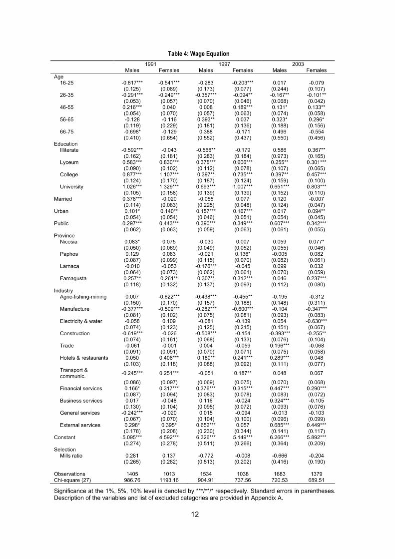
IV. WAGE DECOMPOSITIONS

In order to explain the differences in the wage structure between the two genders, the Oaxaca (1973) decomposition as amended by Neumark (1988) and Oaxaca and Ransom (1994)2 is used. This methodology decomposes the total differences between genders into a portion attributable to differences in the average value of the productive characteristics (the explained part) and a portion attributable to differences in the compensation for productivity characteristics (the unexplained part), which is further broken down as described below:

ˆ ˆ ˆ ˆ( ) ( ) ( ˆ )M F M F N M M N F NW W X X X X Fβ β β β β− = − + − + −

where βΝ is a non-discriminatory coefficient structure. Because no-selection issues based on gender arise, βΝ is estimated by using a pooled regression for males and females. Since no relevant selection issues were found, the analysis below is carried out using the OLS gender equations that are given in Appendix B Table 1. The first term in the above equation measures the explained part, the second term measures the male advantage (i.e. the extent to which the male characteristics are valued above the non-discriminatory coefficient structure) and the third term measures the female disadvantage (i.e. the extent to which the female characteristics are valued below the non-discriminatory coefficient structure).

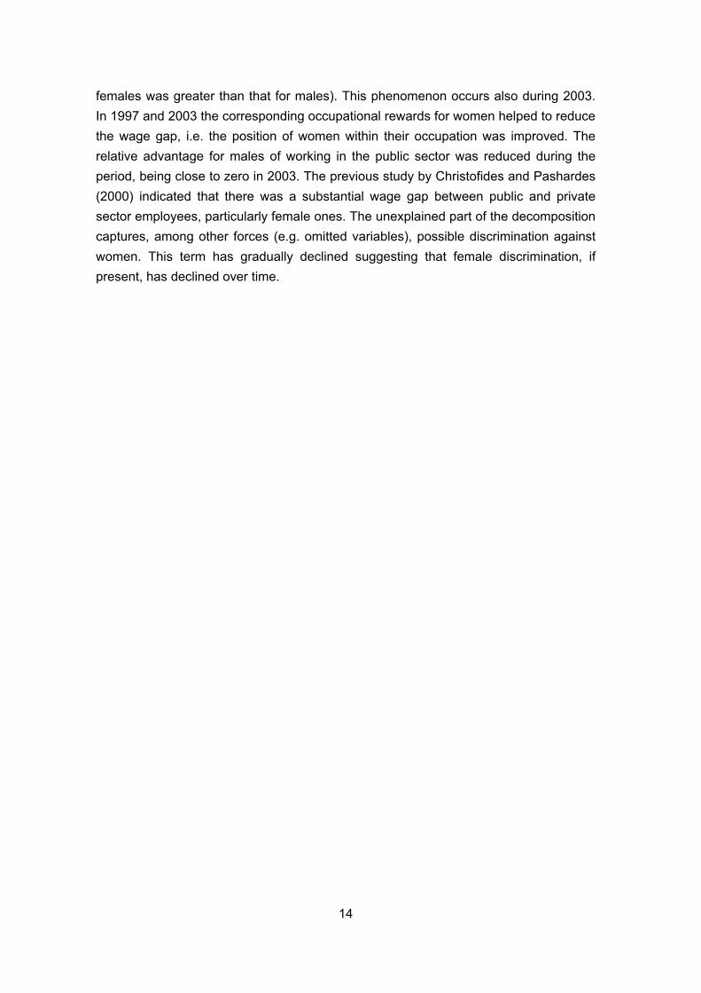
The decomposition results implied by the above equation appear in Table 5. The decomposition is carried out for all three available years. In 1991 the observed mean logarithmic difference is 0.572 units of which 0.161 units represent the explained part (endowment difference) and 0.411 units represent the unexplained part 3 . The decomposition of the endowment difference reveals that the contribution of human capital variables, like education, is smaller compared to industry dummy variables or the public sector dummy. The observed wage gap was substantially lower in 1997. A further, but smaller, reduction to the wage gap occurred in 2003. The large reduction that occurred in 1997 can be partly attributed to the marked rise in the education level of female employees. This is reflected in the decomposition by the negative contribution of education in the gap (which means that the average education level for

2 The analysis was also carried using the methodology proposed by Oaxaca (1973) providing results very close to the results that are presented. 3 The total wage difference for 1991 is close to the result obtained in Christofides and Pashardes (2000), which was 0.532 units. The remaining decomposition results are different, as expected, because of the different explanatory variables used; this was done so as to have consistent variable definitions across Surveys. For the no selection case, the endowment difference in that study was 0.323 units, the male advantage 0.086 units and the female disadvantage 0.125.

13

14

females was greater than that for males). This phenomenon occurs also during 2003. In 1997 and 2003 the corresponding occupational rewards for women helped to reduce the wage gap, i.e. the position of women within their occupation was improved. The relative advantage for males of working in the public sector was reduced during the period, being close to zero in 2003. The previous study by Christofides and Pashardes (2000) indicated that there was a substantial wage gap between public and private sector employees, particularly female ones. The unexplained part of the decomposition captures, among other forces (e.g. omitted variables), possible discrimination against women. This term has gradually declined suggesting that female discrimination, if present, has declined over time.

15

Table 5: Oaxaca-Ransom decomposition

Note: Standard Errors in Parentheses

Year Observed Wage Gap

Total Endowment Difference Education Industry Public Sector Total

Unexplained Part Male Advantage Female Disadvantage

1991 0.572 0.161 0.013 0.018 0.026 0.411 0.172 0.239 (0.039) (0.029) (0.019) (0.014) (0.007) (0.026) (0.025) (0.031)

1997 0.313 -0.028 -0.046 -0.062 0.020 0.341 0.137 0.203 (0.034) (0.025) (0.015) (0.012) (0.007) (0.023) (0.022) (0.025)

2003 0.260 -0.040 -0.014 -0.064 0.007 0.300 0.135 0.165 (0.031) (0.021) (0.012) (0.011) (0.008) (0.023) (0.023) (0.028)

V. THE DISTRIBUTION OF THE WAGE GAP

The decompositions until now have relied on the Ordinary Least Squares (OLS) estimator, which examines how the exogenous variables affect the wage, at the mean of the distribution. By contrast, quantile regression examines the relation between the depended variable and the covariates at various points of the distribution (see Koenker and Bassett (1978)). Thus, it is possible to estimate the effect of gender, education, and other individual characteristics on the ln wage at the bottom of the ln wage distribution (e.g., at the fifth percentile), at the median, and at the top of the distribution (e.g., at the ninety-fifth percentile). In this framework, the samples for the two genders are combined and a single pooled equation is estimated. The following equation is defined:

16

iW X Si i i= β γ ε+ +

where i refers to an individual, W is the observed ln wage, X is a vector of observable characteristics, S is the gender of each individual (adopting a value of one if the individual is male and zero if female) and ε is the residual term. The quantile regression coefficients can be estimated as the solution to:

( )( ), ( ): ( ) ( ) : ( ) ( )

min ( ) ( ) (1 ) ( ) ( )i i i i i i

i i i i i ii W X S i W X S

W X S W X Sβ θ γ θ

β θ γ θ β θ γ θ

θ β θ γ θ θ β θ γ θ≥ + < +

⎧ ⎫⎪ ⎪− − + − − −⎨ ⎬⎪ ⎪⎩ ⎭

∑ ∑

The gender pay gap is given by:

ˆ ˆ ˆ ˆ[ | , 1] [ | , 0]G E W X S E W X S γ= = − = =

This coefficient captures the difference between the two genders and remains unexplained by the observable characteristics. This difference is obtained for each of the three survey years and at different points θ of the wage distribution. The restriction imposed in this specification is that the returns on the individual characteristics are the same across the two genders. An analogous specification has been used in Newell and Reilly (2001) and Albercht et al (2003).

The estimation results for the gender difference γ̂ obtained from the quantile regression are presented in Table 64. In the first column are presented the results obtained estimating the wage equation (1) using the OLS, or mean regression.

γ̂4 Table 6 reports only the results for the estimation of coefficient . The complete estimation results for the rest of the explanatory variables are available from the authors.

17

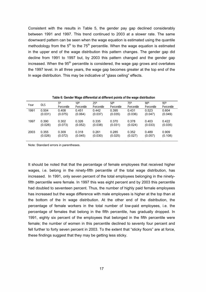
Consistent with the results in Table 5, the gender pay gap declined considerably between 1991 and 1997. This trend continued to 2003 at a slower rate. The same downward pattern can be seen when the wage equation is estimated using the quantile methodology from the 5th to the 75th percentile. When the wage equation is estimated in the upper end of the wage distribution this pattern changes. The gender gap did decline from 1991 to 1997 but, by 2003 this pattern changed and the gender gap increased. When the 95th percentile is considered, the wage gap grows and overtakes the 1997 level. In all three years, the wage gap becomes greater at the top end of the ln wage distribution. This may be indicative of “glass ceiling” effects.

Table 6: Gender Wage differential at different points of the wage distribution

Year OLS 5th Percentile

10th Percentile

25th Percentile

50th Percentile

75th Percentile

90th Percentile

95th Percentile

1991 0.504 0.408 0.451 0.442 0.395 0.431 0.523 0.604 (0.031) (0.075) (0.064) (0.037) (0.035) (0.036) (0.047) (0.049) 1997 0.390 0.302 0.326 0.335 0.370 0.378 0.403 0.422 (0.026) (0.073) (0.052) (0.038) (0.031) (0.024) (0.033) (0.035) 2003 0.355 0.309 0.318 0.261 0.285 0.352 0.489 0.909 (0.026) (0.072) (0.045) (0.030) (0.025) (0.027) (0.057) (0.108)

Note: Standard errors in parentheses.

It should be noted that that the percentage of female employees that received higher wages, i.e. belong in the ninety-fifth percentile of the total wage distribution, has increased. In 1991, only seven percent of the total employees belonging in the ninety-fifth percentile were female. In 1997 this was eight percent and by 2003 this percentile had doubled to seventeen percent. Thus, the number of highly paid female employees has increased but the wage difference with male employees is higher at the top than at the bottom of the ln wage distribution. At the other end of the distribution, the percentage of female workers in the total number of low-paid employees, i.e. the percentage of females that belong in the fifth percentile, has gradually dropped. In 1991, eighty six percent of the employees that belonged in the fifth percentile were female; the number of women in this percentile declined to seventy four percent and fell further to forty seven percent in 2003. To the extent that “sticky floors” are at force, these findings suggest that they may be getting less sticky.

18

VI. CONCLUSIONS

The purpose of this study was to examine the gender wage gap in Cyprus using data from the Cyprus Surveys of Household Expenditure and Income of 1990/91, 1996/97 and 2002/03. Cyprus is consistently rated as one of the EU countries with the highest gender gap. During the negotiations to join the EU, Cyprus introduced a wealth of legislation which aimed to combat this problem. With this legislation, monitoring and enforcement bodies were created and wider public attention turned to this issue.

Previous studies have shown that the usual factors that cause the gender wage gap are not very strong in Cyprus. The female participation rate is high compared to other EU countries, the hours of work similar across genders, and educational attainment for women is comparable that of men. A previous study by Christofides and Pashardes (2002) that used 1991 data showed that a large part of the wage gap cannot be explained by differences in the observable characteristics of the two genders.

Using data from all three Surveys, this study confirmed the existence of a large ln wage gap in 1990/91 (0.571 points), a substantial part of which (0.161 ln wage points) could be explained by the more favourable productive characteristics for men. By 1996/97, the ln wage gap fell to 0.313 and, by the 2002/03 survey, to 0.260. There has, therefore, been a substantial improvement in the observed or unconditional gap. However, by 1996/97, the characteristics of women had improved to such an extent that no part of the remaining 0.313 points could be explained by differences in characteristics. This also holds for the observed 2002/03 gap. Whether these remaining pay gaps reflect unmeasurable characteristics or discrimination, remains a moot point.

The quantile regression analysis suggests that the improvement in the observed ln wage gap was felt throughout the ln wage distribution up until the 90th percentile. The gender pay gaps declined and a smaller proportion of the individuals at the bottom of the distribution were women. However, at the 90th and 95th percentiles, the wage gap increased. This may reflect “glass ceiling” effects, though it must be remembered that the sample of men and women at the extreme of the wage distribution may be rather unusual.

Future studies should examine further these high-flying populations. Another extension of this study might have been to use a different decomposition analysis to examine how the change in individual characteristics over time has contributed to the formation of the gender wage gap. The method that has traditionally been used to this end is that of Juhn et al (1991). However, this method has been criticized by Suen (1997) and Yun

19

(2007) because of the underlying assumptions that it uses. These criticisms do not impinge on the decompositions in section IV.

REFERENCES

Albrecht J., A. Bjorklund and S. Vroman (2003), “Is there a Glass Ceiling in Sweden?” Journal of Labor Economics 21 (1) : 145–177.

Blau, F. D. and L. M. Kahn. (1997), “Swimming Upstream: Trends in the Gender Wage Differential in the 1980s”, Journal of Labor Economics, 15:l pt. 1, pp. 1-42.

Christofides, L. N. and P. Pashardes (2002), “Self/Paid Employment, Public/Private Sector Selection, and Wage Differentials”, Labour Economics, 9, pp. 737-762.

Christofides, L. N. and P. Pashardes (2000), “Development and the Gender Wage Gap: A Study of Paid Work in Cyprus”, Labour, pp. 311-329.

Juhn, C., K. M. Murphy, and B. Pierce (1991), “Accounting for the Slowdown in Black-White Wage Convergence” In Workers and Their Wages, edited by Marvin Kosters, (AEI Press, Washington, DC), pp. 107-43.

Koenker, R., and G. Bassett (1978), “Regression Quantiles.” Econometrica 46, pp. 33–50.

Neumark, D. (1988), “Employer’s Discriminatory Behavior and the Estimation of Wage Discrimination”, The Journal of Human Resources, XXIII, pp. 279-295.

Newell A. and B. Reilly (2001), “The Gender Pay Gap in the Transition from Communism: Some Empirical Evidence”. Economic Systems 25: pp. 287–304

Oaxaca, R. L. (1973), “Male-Female Wage Differentials in Urban Labour Markets”, International Economic Review, Vol. 14, pp. 693-709.

Oaxaca, R. L. and M. R. Ransom (1994), “On Discrimination and the Decomposition of Wage Differentials”, Journal of Econometrics, Vol. 61, pp. 5-21.

Panayiotou, A. (2006), “The gender pay gap in Cyprus: Origins and policy responses”, External report commissioned by and presented to the EU Directorate-general Employment and Social Affairs, Unit G1 “Equality between women and men”.

Suen, W. (1997), “Decomposing Wage residuals: Unmeasured Skill or Statistical Artifact?” Journal of Labor Economics, 15(3), pp. 555-566.

Yun, M. S. (2007) “Wage Differentials, Discrimination and Inequality: A Cautionary Note on the Juhn, Murphy and Pierce Decomposition Method”, IZA Discussion Paper, No. 2937.

20

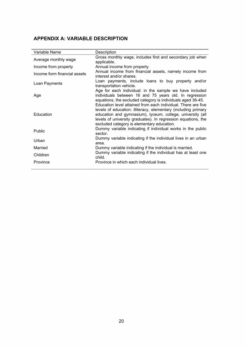
APPENDIX A: VARIABLE DESCRIPTION

Variable Name Description

Average monthly wage Gross monthly wage, includes first and secondary job when applicable.

Income from property Annual income from property.

Income form financial assets Annual income from financial assets, namely income from interest and/or shares.

Loan Payments Loan payments, include loans to buy property and/or transportation vehicle.

Age Age for each individual: in the sample we have included individuals between 16 and 75 years old. In regression equations, the excluded category is individuals aged 36-45.

Education

Education level attained from each individual. There are five levels of education: illiteracy, elementary (including primary education and gymnasium), lyceum, college, university (all levels of university graduates). In regression equations, the excluded category is elementary education.

Public Dummy variable indicating if individual works in the public sector.

Urban Dummy variable indicating if the individual lives in an urban area.

Married Dummy variable indicating if the individual is married.

Children Dummy variable indicating if the individual has at least one child.

Province Province in which each individual lives.

21

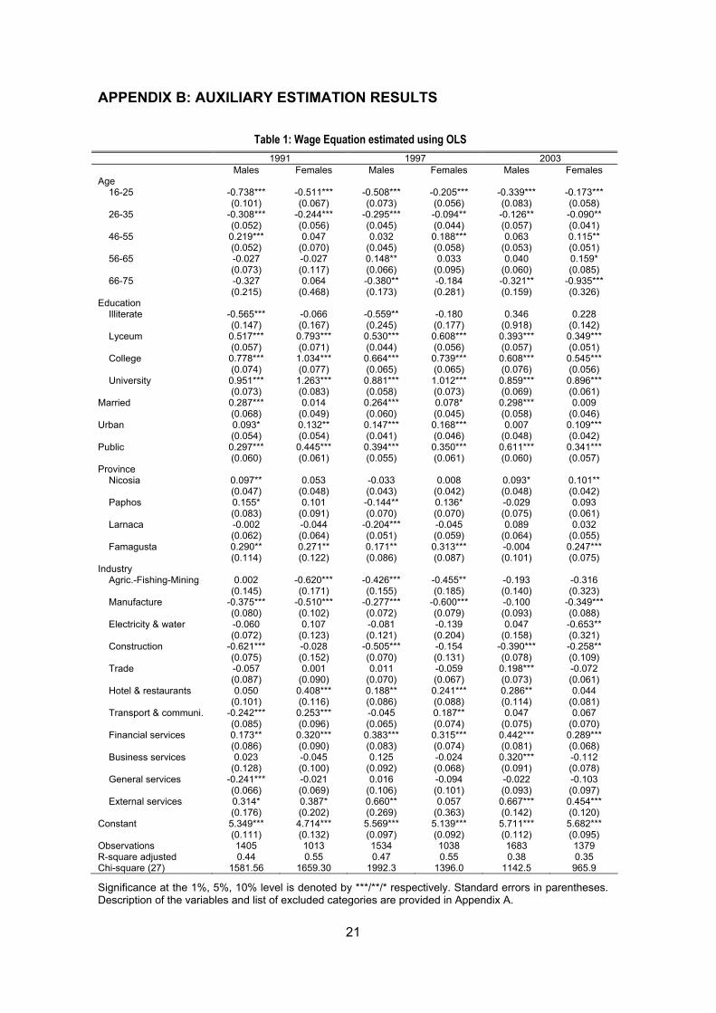
APPENDIX B: AUXILIARY ESTIMATION RESULTS

Table 1: Wage Equation estimated using OLS 1991 1997 2003

Males Females Males Females Males Females Age

16-25 -0.738*** -0.511*** -0.508*** -0.205*** -0.339*** -0.173*** (0.101) (0.067) (0.073) (0.056) (0.083) (0.058) 26-35 -0.308*** -0.244*** -0.295*** -0.094** -0.126** -0.090** (0.052) (0.056) (0.045) (0.044) (0.057) (0.041) 46-55 0.219*** 0.047 0.032 0.188*** 0.063 0.115** (0.052) (0.070) (0.045) (0.058) (0.053) (0.051) 56-65 -0.027 -0.027 0.148** 0.033 0.040 0.159* (0.073) (0.117) (0.066) (0.095) (0.060) (0.085) 66-75 -0.327 0.064 -0.380** -0.184 -0.321** -0.935***

(0.215) (0.468) (0.173) (0.281) (0.159) (0.326) Education

Illiterate -0.565*** -0.066 -0.559** -0.180 0.346 0.228 (0.147) (0.167) (0.245) (0.177) (0.918) (0.142) Lyceum 0.517*** 0.793*** 0.530*** 0.608*** 0.393*** 0.349*** (0.057) (0.071) (0.044) (0.056) (0.057) (0.051) College 0.778*** 1.034*** 0.664*** 0.739*** 0.608*** 0.545*** (0.074) (0.077) (0.065) (0.065) (0.076) (0.056) University 0.951*** 1.263*** 0.881*** 1.012*** 0.859*** 0.896***

(0.073) (0.083) (0.058) (0.073) (0.069) (0.061) Married 0.287*** 0.014 0.264*** 0.078* 0.298*** 0.009 (0.068) (0.049) (0.060) (0.045) (0.058) (0.046) Urban 0.093* 0.132** 0.147*** 0.168*** 0.007 0.109*** (0.054) (0.054) (0.041) (0.046) (0.048) (0.042) Public 0.297*** 0.445*** 0.394*** 0.350*** 0.611*** 0.341***

(0.060) (0.061) (0.055) (0.061) (0.060) (0.057) Province

Nicosia 0.097** 0.053 -0.033 0.008 0.093* 0.101** (0.047) (0.048) (0.043) (0.042) (0.048) (0.042) Paphos 0.155* 0.101 -0.144** 0.136* -0.029 0.093 (0.083) (0.091) (0.070) (0.070) (0.075) (0.061) Larnaca -0.002 -0.044 -0.204*** -0.045 0.089 0.032 (0.062) (0.064) (0.051) (0.059) (0.064) (0.055) Famagusta 0.290** 0.271** 0.171** 0.313*** -0.004 0.247***

(0.114) (0.122) (0.086) (0.087) (0.101) (0.075) Industry

Agric.-Fishing-Mining 0.002 -0.620*** -0.426*** -0.455** -0.193 -0.316 (0.145) (0.171) (0.155) (0.185) (0.140) (0.323) Manufacture -0.375*** -0.510*** -0.277*** -0.600*** -0.100 -0.349*** (0.080) (0.102) (0.072) (0.079) (0.093) (0.088) Electricity & water -0.060 0.107 -0.081 -0.139 0.047 -0.653** (0.072) (0.123) (0.121) (0.204) (0.158) (0.321) Construction -0.621*** -0.028 -0.505*** -0.154 -0.390*** -0.258** (0.075) (0.152) (0.070) (0.131) (0.078) (0.109) Trade -0.057 0.001 0.011 -0.059 0.198*** -0.072 (0.087) (0.090) (0.070) (0.067) (0.073) (0.061) Hotel & restaurants 0.050 0.408*** 0.188** 0.241*** 0.286** 0.044 (0.101) (0.116) (0.086) (0.088) (0.114) (0.081) Transport & communi. -0.242*** 0.253*** -0.045 0.187** 0.047 0.067 (0.085) (0.096) (0.065) (0.074) (0.075) (0.070) Financial services 0.173** 0.320*** 0.383*** 0.315*** 0.442*** 0.289*** (0.086) (0.090) (0.083) (0.074) (0.081) (0.068) Business services 0.023 -0.045 0.125 -0.024 0.320*** -0.112 (0.128) (0.100) (0.092) (0.068) (0.091) (0.078) General services -0.241*** -0.021 0.016 -0.094 -0.022 -0.103 (0.066) (0.069) (0.106) (0.101) (0.093) (0.097) External services 0.314* 0.387* 0.660** 0.057 0.667*** 0.454***

(0.176) (0.202) (0.269) (0.363) (0.142) (0.120) Constant 5.349*** 4.714*** 5.569*** 5.139*** 5.711*** 5.682***

(0.111) (0.132) (0.097) (0.092) (0.112) (0.095) Observations 1405 1013 1534 1038 1683 1379 R-square adjusted 0.44 0.55 0.47 0.55 0.38 0.35 Chi-square (27) 1581.56 1659.30 1992.3 1396.0 1142.5 965.9

Significance at the 1%, 5%, 10% level is denoted by ***/**/* respectively. Standard errors in parentheses. Description of the variables and list of excluded categories are provided in Appendix A.

22

Table 2: Wage Equation estimated using the ML methodology 1991 1997 2003

Males Females Males Females Males Females Age

16-25 -0.761*** -0.519*** -0.475*** -0.204*** -0.275*** -0.145** (0.098) (0.066) (0.083) (0.058) (0.087) (0.062) 26-35 -0.303*** -0.246*** -0.304*** -0.094** -0.134** -0.093** (0.050) (0.055) (0.046) (0.044) (0.059) (0.040) 46-55 0.218*** 0.045 0.028 0.189*** 0.075 0.120** (0.053) (0.066) (0.044) (0.057) (0.052) (0.050) 56-65 -0.057 -0.049 0.184** 0.035 0.091 0.199** (0.078) (0.124) (0.080) (0.095) (0.063) (0.094) 66-75 -0.436* 0.016 -0.266 -0.180 -0.174 -0.821***

(0.225) (0.428) (0.237) (0.259) (0.164) (0.254) Education

Illiterate -0.573*** -0.060 -0.560** -0.179 0.388 0.269** (0.129) (0.163) (0.238) (0.165) (0.815) (0.125) Lyceum 0.536*** 0.802*** 0.507*** 0.607*** 0.368*** 0.335*** (0.060) (0.069) (0.051) (0.055) (0.057) (0.053) College 0.807*** 1.052*** 0.624*** 0.738*** 0.570*** 0.519*** (0.079) (0.080) (0.080) (0.071) (0.077) (0.063) University 0.973*** 1.279*** 0.853*** 1.010*** 0.822*** 0.868***

(0.076) (0.085) (0.065) (0.077) (0.067) (0.067) Married 0.314*** 0.005 0.216*** 0.077* 0.266*** 0.004 (0.072) (0.050) (0.081) (0.043) (0.059) (0.046) Urban 0.095* 0.134** 0.148*** 0.168*** 0.009 0.104** (0.051) (0.053) (0.040) (0.045) (0.047) (0.043) Public 0.297*** 0.444*** 0.394*** 0.350*** 0.611*** 0.342***

(0.062) (0.063) (0.056) (0.061) (0.059) (0.055) Province

Nicosia 0.093** 0.059 -0.032 0.008 0.087* 0.094** (0.046) (0.048) (0.042) (0.042) (0.047) (0.042) Paphos 0.147* 0.097 -0.126* 0.136** -0.025 0.090 (0.083) (0.088) (0.073) (0.067) (0.076) (0.058) Larnaca -0.004 -0.046 -0.200*** -0.045 0.091 0.032 (0.063) (0.066) (0.051) (0.057) (0.062) (0.054) Famagusta 0.280** 0.269** 0.191** 0.313*** 0.005 0.244***

(0.111) (0.121) (0.089) (0.082) (0.097) (0.073) Industry

Agric.-fishing-mining 0.003 -0.620*** -0.428*** -0.455** -0.194 -0.315 (0.147) (0.164) (0.150) (0.179) (0.140) (0.300) Manufacture -0.376*** -0.510*** -0.278*** -0.600*** -0.100 -0.348*** (0.080) (0.102) (0.074) (0.079) (0.091) (0.088) Electricity & water -0.060 0.108 -0.081 -0.139 0.049 -0.647*** (0.067) (0.104) (0.123) (0.182) (0.152) (0.062) Construction -0.620*** -0.028 -0.505*** -0.154 -0.390*** -0.257** (0.072) (0.153) (0.068) (0.122) (0.076) (0.107) Trade -0.058 0.001 0.010 -0.059 0.198*** -0.070 (0.085) (0.090) (0.070) (0.068) (0.073) (0.061) Hotel & restaurants 0.050 0.407*** 0.187** 0.241*** 0.287** 0.046 (0.100) (0.115) (0.088) (0.088) (0.113) (0.077) Transport & communi.

-0.243*** 0.252*** -0.046 0.187*** 0.047 0.067

(0.087) (0.094) (0.066) (0.073) (0.071) (0.069) Financial services 0.171** 0.319*** 0.381*** 0.315*** 0.443*** 0.289*** (0.084) (0.093) (0.081) (0.075) (0.081) (0.068) Business services 0.021 -0.046 0.122 -0.024 0.320*** -0.110 (0.125) (0.102) (0.091) (0.069) (0.092) (0.079) General services -0.241*** -0.021 0.017 -0.094 -0.021 -0.103 (0.064) (0.069) (0.106) (0.098) (0.092) (0.095) External services 0.309* 0.389** 0.658*** 0.057 0.671*** 0.453***

(0.166) (0.197) (0.204) (0.310) (0.136) (0.110) Constant 5.274*** 4.683*** 5.682*** 5.142*** 5.810*** 5.745***

(0.130) (0.139) (0.160) (0.116) (0.113) (0.109)

Observations 1405 1013 1534 1038 1683 1379 Chi-square (27) 1374.2 1452.52 1395.45 1395.45 984.54 891.89 Rho ( ρ ) 0.118 0.056 -0.179 -0.005 -0.157 -0.102 Test (p-value) 0 : 0H ρ = 0.264 0.600 0.396 0.967 0.03 0.333

Significance at the 1%, 5%, 10% level is denoted by ***/**/* respectively. Standard errors in parentheses. Description of the variables and list of excluded categories are provided in Appendix A.

23

Recent Economic Policy/Analysis Papers

09-07 Eliophotou–Menon Μ., N. Pashourtidou, A. Polykarpou and M. Socratous, “Students’ employment and earnings expectations in Cyprus”, December 2007 – in Greek.

08-07 Mamuneas T. and C.S. Savva, "Public expenditure in infrastructure and the

productivity of the private sector", November 2007 – in Greek. 07-07 Athanasiadou Μ., T. Mamuneas and C.S. Savva, "R&D in Cyprus and the

EU", October 2007 – in Greek. 06-07 Kontolemis Ζ., "Economic forecasts", July 2007. 05-07 Christofides L., A. Kourtellos and K. Vrachimis, "New unemployment indices

for Cyprus and their performance in established economic relationships", July 2007.

04-07 Mamuneas T. and C.S. Savva, "The efficiency of Cypriot commercial banks:

Comparison with Greece and the UK", June 2007. 03-07 Hassapis C., "Inflation, Long Term Interest Rate Convergence and the

Maastricht Criteria", April 2007 – in Greek. 02-07 Pashardes P., S. Hajispyrou and N. Nicolaidou, "Poverty in Cyprus: 1991-

2003", March 2007 – in Greek. 01-07 Christofides L., A. Kourtellos and K. Vrachimis, "Unemployment indices for

Cyprus: A comparative study", March 2007. 13-06 Christofides L., A. Kourtellos and I. Stylianou, "Approaches towards the

development of a model of the Cyprus economy", December 2006 – in Greek. 12-06 Stephanou C. and D. Vittas, "Public debt management and debt market

development in Cyprus: Evolution, current challenges and policy options", December 2006.

11-06 Michael Μ., L. Christofides, C. Hadjiyiannis, S. Clerides, Μ. Stephanides and

Μ. Michalopoulou, "The effect of immigration on the wages of Cypriot workers", October 2006 – in Greek.

10-06 Kontolemis Z., S. Hajispyrou and D. Komodromou, "Labour participation:

gender and age differentials", October 2006 – in Greek. 09-06 Zachariadis T., "Long-term forecast of electricity consumption in Cyprus", July

2006 – in Greek.