Econometric Modeling

Solutions to Exercises with Even Numbers

David F. HendryBent Nielsen

24 January 2008 - preliminary version

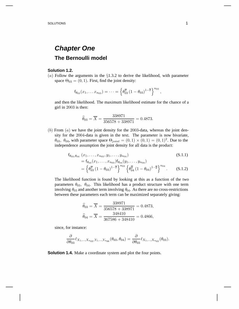
SOLUTIONS 1

Chapter OneThe Bernoulli model

Solution 1.2.(a) Follow the arguments in the §1.3.2 to derive the likelihood, with parameter

space Θ03 = (0, 1). First, find the joint density:

fθ03(x1, . . . xn03) = · · · ={

θx03 (1 − θ03)

1−x}n03

,

and then the likelihood. The maximum likelihood estimate for the chance of agirl in 2003 is then:

θ03 = X =338971

356578 + 338971= 0.4873.

(b) From (a) we have the joint density for the 2003-data, whereas the joint den-sity for the 2004-data is given in the text. The parameter is now bivariate,θ03, θ04, with parameter space Θjoint = (0, 1) × (0, 1) = (0, 1)2. Due to theindependence assumption the joint density for all data is the product:

fθ03,θ04 (x1, . . . , xn03 , y1, . . . , yn04) (S.1.1)

= fθ03(x1, . . . , xn03)fθ04(y1, . . . , yn04)

={

θx03 (1 − θ03)

1−x}n03

{θy04 (1 − θ04)

1−y}n04

. (S.1.2)

The likelihood function is found by looking at this as a function of the twoparameters θ03, θ04. This likelihood has a product structure with one terminvolving θ03 and another term involving θ04. As there are no cross-restrictionsbetween these parameters each term can be maximized separately giving:

θ03 = X =338971

356578 + 338971= 0.4873,

θ04 = X =348410

367586 + 348410= 0.4866,

since, for instance:

∂

∂θ03�X1,...,Xn03 ,Y1,...,Yn98

(θ03, θ04) =∂

∂θ03�X1,...,Xn03

(θ03).

Solution 1.4. Make a coordinate system and plot the four points.

2 SOLUTIONS

(a) Use (1.2.3) so:

P(X = −1) = P(X = −1, Y = 0) =14,

P(X = 0) = P(X = 0, Y = −1) + P(X = 0, Y = 1) =12,

P(X = 1) = P(X = 1, Y = 0) =14.

(b) No. Note that Y has the same marginal distribution as X. Then it holds, forinstance that:

P(X = 1, Y = 0) =14�= P(X = 1)P(Y = 0) =

(14

)(12

)=

18.

In order to have independence it is necessary that the two variables vary in aproduct space. Here the sample space is like a rhomb rather than a square.

Chapter TwoInference in the Bernoulli model

Solution 2.2. These data can be analyzed using the Bernoulli model. Thus, thechance of a newborn child being female is estimated by:

θ =1964

1964 + 2058= 0.4883

As the data in Table 1.6 are measured in thousands, then:

n = (1964 + 2058) × 1000 = 4022000.

The fact that the reported data are in thousands simply results in a roundingerror of up to 1000, corresponding to a relative error of 0.00025. Thus, inreporting the estimate for θ the rounding error kicks in on the fourth digit afterthe decimal point.The standard error of the estimate for θ is:

se(θ) =

√θ(1 − θ)√

n=

√0.4883(1 − 0.4883)√

4022000= 0.000249,

Since the 99.5%-quantile of the standard normal distribution is 2.576 (see Ta-ble 2.1) this gives a 99%-confidence interval of:

0.4883 − 2.576 × 0.000249 ≤ θ ≤ 0.4883 + 2.576 × 0.000249,

or:

0.4877 ≤ θ ≤ 0.4889.

SOLUTIONS 3

This confidence interval overlaps with the confidence interval for the UK re-ported in §2.3.1, indicating that sex ratios are not all that different betweencountries. A formal test could be made as set out in Exercise 2.3.

Solution 2.4. Suppose XD= Bernoulli[p]. Then:

E (X) = 0 · (1 − p) + 1 · p = p,

Var (X) = (0 − p)2 · (1 − p) + (1 − p)2 · p= p2 (1 − p) + p (1 − p) = p (1 − p) .

The variance can also be found from the general formula:

E{X − E(X)}2 = E[X2 − 2XE(X) + {E(X)}2] = E(X2)− {E(X)}2.

using that for the Bernoulli case:

E(X2)

= 02 · (1 − p) + 12 · p = p.

Choosing a success probability p the density and distribution functions are:

f(x) =

⎧⎨⎩ 1 − p for x = 0,p for x = 1,0 otherwise,

F(x) =

⎧⎨⎩ 0 for x < 0,1 − p for 0 ≤ x < 1,1 for 1 ≤ x.

Now, the “confidence intervals” are, for k = 1, 2:

E (X) ± ksdv (X) = p ± k√

p (1 − p).

Examples:Let p = 1/2 then E (X) = 1/2, sdv (X) = 1/2 so E (X) ± sdv (X) hasprobability 0 (if open interval) while E (X) ± 2sdv (X) has probability 1.let p = 1/5 then E (X) = 1/5, sdv (X) = 2/5 so E (X) ± sdv (X) hasprobability 4/5 while E (X) ± 2sdv (X) has probability 1.

Solution 2.6. Use that expectations are linear operators, and that the expectation,E(X), is deterministic:

E{X − E(X)}2

= [ complete square ] = E[X2 − 2XE(X) + {E(X)}2]= [ linearity ] = E(X2) − 2{E(X)}2 + {E(X)}2 = E(X2) − {E(X)}2.

Solution 2.8. The key to the solution is (2.1.8) stating that:

X,Y independent ⇒ E(XY ) = E(X)E(Y ).

4 SOLUTIONS

In particular, for constants μx, μy:

X,Y independent

⇔ (X − μx), (Y − μy) independent

⇒ E{(X − μx)(Y − μy)} = E(X − μx)E(Y − μy).

Thus, the problem can be solved as follows:

Cov(X,Y )= [ Definition (2.1.12)] = E[{X − E(X)}{Y − E(Y )}]= [ use independence and (2.1.8)] = E{X − E(X)}E{Y − E(Y )}= [ use E{X − E(X)} = E(X) − E(X) = 0} ] = 0.

Solution 2.10.(a) This is a straight forward application of the Law of Large Numbers. For in-

stance, the first subsample consists of n/2 independently identical distributedvariables. Thus, their sample average, here denoted Z1 converges in probabil-ity to their population expectation, θ1 = 1/4.

(b) Here the definition of convergence in probability as stated in Theorem 2.1 hasto be used. Thus, it has to be shown that for any δ > 0 the probability that:∣∣∣∣Y − 1

2

∣∣∣∣ > δ

converges to zero. Now, decompose:

Y =1n

n∑i=1

Yi =1n

n/2∑i=1

Yi +1n

n∑i=n/2+1

Yi

=(

12

)2n

n/2∑i=1

Yi +(

12

)2n

n∑i=n/2+1

Yi =Z1

2+

Z1

2.

Likewise, decompose 1/2 = (1/2)(1/4) + (1/2)(3/4), so:

Y − 12

=12

(Z1 − θ1) +12

(Z2 − θ2) .

In particular, by the triangle inequality:∣∣∣∣Y − 12

∣∣∣∣ ≤ 12|Z1 − θ1| + 1

2|Z2 − θ2| .

SOLUTIONS 5

Since Z1, Z2 both converge in probability, then for any δ it holds that:

P

(∣∣∣∣Y − 12

∣∣∣∣ > δ

)≤P

(12|Z1 − θ1| + 1

2|Z2 − θ2| > δ

)≤ [ check ]

≤P

(12|Z1 − θ1| >

δ

2or

12|Z2 − θ2| >

δ

2

)= P (|Z1 − θ1| > δ or |Z2 − θ2| > δ) .

Now, the so-called Boole’s inequality is needed. This states that for any eventsA, B then:

P(A or B) ≤ P(A) + P(B). (S.2.1)

This comes about as follows. If A and B are disjoint, that is, they cannot bothbe true, then (S.2.1) holds with equality. This property was used when link-ing distribution functions and densities in §1.2.2. If A and B are not disjoint,split the sets into three disjoint parts: (A but not B), (B but not A), (A and B).Then the left hand side of (S.2.1) includes these sets once each, whereas theright hand side includes the intersection set (A and B) twice, hence the in-equality.Applying Boole’s inequality it then holds:

P

(∣∣∣∣Y − 12

∣∣∣∣ > δ

)≤ P (|Z1 − θ1| > δ) + P (|Z2 − θ2| > δ) .

Due to (a) both of the probabilities on the right hand side converge to zero.(c) The Law of Large Numbers requires that the random variables are indepen-

dent, which is satisfied here, as well as having the same distribution, whichis not satisfied here. The theorem therefore does not apply to the full set ofobservations in this case. As all inference in a given statistical model is basedon the the Law of Large Numbers and the Central Limit Theorem, it is there-fore important to check model assumptions. The inference may be valid undermilder assumptions, but this is not always the case.

Chapter ThreeA first regression model

Solution 3.2. Recall β = 5.02 and σ = 0.753.

n = 100 4.86 < β < 5.17,n = 10000 5.00 < β < 5.04.

The widths of the confidence intervals vary with√

n.

6 SOLUTIONS

Solution 3.4.(a) The first order derivative is given in (3.3.8). Thus the second derivative is:

∂2

∂ (σ2)2�Y1,...,Yn

(β, σ2

)=

n

2σ4− 1

σ6

n∑i=1

u2i =

n

2σ6

(σ2 − 2σ2

),

giving that the second order condition is satisfied at σ2 since:

n

2σ6

(σ2 − 2σ2

)= − n

2σ6σ2 = − n

2σ4< 0.

Therefore the profile likelihood is locally concave. It is not, however, globallyconcave, since the second derive is positive for σ2 > 2σ2. To show uniquenessof the maximum likelihood estimator, global concavity is not needed, however.Since ∂�/∂σ2 is positive for σ2 < σ2 and negative for σ2 > σ2 then σ2 is aglobal maximum.Note: This argument shows that there is a unique mode for the likelihood.

(b) The profile log-likelihood for θ = log σ is found by reparametrizing (3.3.7):

�Y1,...Yn(β, log σ) = −n log σ −n∑

i=1

u2i /(2σ

2).

Thus the profile log-likelihood for θ is:

�Y1,...Yn(β, θ) = −nθ − exp(−2θ)n∑

i=1

u2i /2,

with derivatives:

∂�/∂θ =−n + exp(−2θ)n∑

i=1

u2i ,

∂2�/∂θ2 =−2 exp(−2θ)n∑

i=1

u2i .

The second derivative is negative for all θ. Thus the profile log-likelihood forθ is concave with a unique maximum.Note: This argument shows that with the θ = log σ parametrization the like-lihood is concave. In particular, there is a unique mode. Concavity is notinvariant to reparametrization, whereas uniqueness of the mode is invariant.

Solution 3.6. We know that if XD= N[μ, σ2] then E (X) = μ, Var (X) = σ2 so

by (2.1.6) and (2.1.10) we have E (aX + b) = aμ+b and Var(aX+b) = a2σ2.

Solution 3.8. Use Table 2.1.(a) Due to the symmetry then P(X ≤ 0) = 1/2. Since P(X > 2.58) = 0.005

then the lower quantile satisfies P(0 < X ≤ 2.58) = 0.995.

SOLUTIONS 7

(b) Note that X = (Y − 4)/√

4 = (Y − 4)/2 D= N[0, 1]. Therefore:

P(Y < 0) = P

(Y − 4

2<

0 − 42

)= P(X < −2)

Now, using that the normal distribution is symmetric it follows that:

P(Y < 0) = P(X < −2) = P(X > 2) ≈ 0.025

Finally, we want to find a quantile q so P(Y > q) = 0.025. The standardnormal table gives P(X > 2) = 1.96. As Y = 2X + 4 the 97.5%-quantile forY is then 2 × 1.96 + 4 = 7.92.

Solution 3.10. We have β =∑n

i=1 Yixi/(∑n

i=1 x2i ) where x1, . . . xn are non-

random constants. The only source of randomness is therefore the Yis. Thus βis a linear combination of independent normal distributed variables and mustbe normally distributed, see (3.4.5). Therefore we only need to find the expec-tation and variance of β using the formulas for the expectation and variance ofsums, (2.1.7), (2.1.11). First the expectation:

E(β1)= [ (2.1.7) ] =∑n

i=1 xiE (Yi)∑ni=1 x2

i

= [ model : YiD= N[βxi, σ

2] so E(Yi) = βxi ]

=∑n

i=1 xiβxi∑ni=1 x2

i

= β,

and similarly the variance:

Var(β1)= [ (2.1.14) using independence ] =∑n

i=1 x2i Var (Yi)

(∑n

i=1 x2i )2

= [ model : YiD= N[βxi, σ

2] so Var(Yi) = σ2 ]

=∑n

i=1 x2i σ

2

(∑n

i=1 x2i )2

=σ2∑ni=1 x2

i

.

Solution 3.12.(a) The joint density is:

fλ(y1, . . . , yn) = [ independence, use (3.2.1) ] =n∏

i=1

fλ(yi)

= [ Poisson distribution ] =n∏

i=1

λyi

yi!exp(−λ).

Using the functional equation for powers, see (1.3.1), this can be rewritten as:

fλ(y1, . . . , yn) = λ∑n

i=1 yi exp(−nλ)n∏

i=1

1yi!

={λy exp(−λ)

}nn∏

i=1

1yi!

,

8 SOLUTIONS

where y = n−1∑n

i=1 yi is the average of y1, . . . , yn. The likelihood functionis then:

LY1,...,Yn(λ) ={λY exp(−λ)

}nn∏

i=1

1Yi!

,

with the corresponding log-likelihood function:

�Y1,...,Yn(λ) = n log{λY exp(−λ)

}+ log

(n∏

i=1

1Yi!

)= [ functional equation for logarithm, (1.3.5) ]

= n{Y log(λ) − λ

}− n∑i=1

log(Yi!).

(b) The maximum likelihood equation is found by differentiating the log-likelihoodfunction �:

∂

∂λ�Y1,...,Yn(λ) = n

(Y

λ− 1)

,

giving the likelihood equation:

n

(Y

λ− 1)

= 0,

which is solved by λ = Y . To show that the solution is unique note either thatthe first derivative of � is positive for λ < λ and negative for λ > λ or find thesecond derivative:

∂2

∂λ2�Y1,...,Yn(λ) = −n

Y

λ2,

which is negative for all values of λ so the log-likelihood function is concave.Note, that these arguments only apply for Y > 0. If, however, Y = 0 there isno variation to model.

Chapter FourThe logit model

Solution 4.2. Use (4.2.4) and (4.2.5) to see that:

P(Yi = 0|Xi) = [ (4.2.5) ] = P(Y ∗i < 0|Xi)

= [ (4.2.4) ] = P(β1 + β2Xi + ui < 0|Xi)= P(ui < −β1 − β2Xi|Xi).

SOLUTIONS 9

Using the definition of the logistic distribution, which is continuous, we get:

P(Yi = 0|Xi) =exp(−β1 − β2Xi)

1 + exp(−β1 − β2Xi).

Extend the fraction by exp(β1 + β2Xi) and use the functional equation forpowers, see (1.3.1), to get:

P(Yi = 0|Xi) =1

exp(β1 + β2Xi) + 1.

In particular:

P(Yi = 1|Xi) = 1 − P(Yi = 0|Xi) =exp(β1 + β2Xi)

1 + exp(β1 + β2Xi)

as desired.

Solution 4.4. Without loss of generality we can assume that the observations areordered so the first m regressors Xi are all 1. Then (4.2.8), (4.2.9) reduce as:

mexp

(β1 + β2

)1 + exp

(β1 + β2

) + (n − m)exp

(β1

)1 + exp

(β1

) =n∑

i=1

Yi, (S.4.1)

mexp

(β1 + β2

)1 + exp

(β1 + β2

) =m∑

i=1

Yi. (S.4.2)

Subtracting equation (S.4.2) from (S.4.1) shows :

(n − m)exp

(β1

)1 + exp

(β1

) =n∑

i=m+1

Yi.

Since the function y = g(x) = exp(x)/{1 + exp(x)} has the inverse x =g−1(y) = log{y/(1 − y)} this implies:

β1 = log(n − m)−1

∑ni=m+1 Yi

1 − (n − m)−1∑n

i=m+1 Yi.

Correspondingly, from (S.4.2):

β1 + β2 = logm−1

∑mi=1 Yi

1 − m−1∑m

i=1 Yi,

and thus:

β2 = logm−1

∑mi=1 Yi

1 − m−1∑m

i=1 Yi− log

(n − m)−1∑n

i=m+1 Yi

1 − (n − m)−1∑n

i=m+1 Yi.

10 SOLUTIONS

Solution 4.6.(a) Inspect that inserting the expression for pi = p(Xi) in (4.2.6), (4.2.7) gives the

desired answer.(b) This follows by noting that:

E(Yi | I) = pi, E(YiXi | I) = piXi,

(c) The key to the result is that:

∂

∂β1pi = pi(1 − pi),

∂

∂β1pi = pi(1 − pi)Xi,

Apply this to the first derivatives given in (a).(d) Start with the element ∂2

∂β21�(β1, β2). Since 0 < pi < 1 the diagonal terms

this equals minus one times a sums of positive elements. When it comes to∂2

∂β22�(β1, β2) the summands are zero if Xi = 0. Provided the Xis are not all

zero the overall sum is positive.(e) By the Cauchy-Schwarz inequality:{

n∑i=1

pi(1 − pi)Xi

}2

=

{n∑

i=1

√pi(1 − pi)

√pi(1 − pi)Xi

}2

≤{

n∑i=1

pi(1 − pi)

}{n∑

i=1

pi(1 − pi)Xi

},

with identity only if pi(1 − pi) = pi(1 − pi)Xi for all i, that is if Xi = 1 forall i.

Chapter FiveThe two-variable regression model

Solution 5.2. On the one hand, if (Yi|Xi)D= N[β1 + β2Xi, σ

2] is the correctmodel with β1 �= 0, it must be a bad idea to use the simpler model! We willreturn to that issue in connection with omitted variable bias. On the other handif the simple model is correct this must be better to use. We will return tothat issue in connection with efficiency. In practice it is extremely rare to havemodels with regressors, but no intercept. When it comes to time series modelswithout intercepts are often used in expositions, but rarely in practiceIf it is deemed appropriate to omit the intercept a complication one has to becareful with using the standard output of econometric and statistical software.While the estimators and t-statistics are fine, a few statistics are not applicablein the usual way for models without an intercept. This applies for instance tothe R2-statistic and to Q-Q plots (see Engler and Nielsen, 2007 for the latter).

SOLUTIONS 11

Solution 5.4. From (5.2.1) we have:

β1 = Y − β2X, β2 =n∑

i=1

Yi

(Xi − X

)∑nj=1

(Xj − X

)2 .

Therefore:

β1 = Y − X

∑ni=1 Yi

(Xi − X

)∑nj=1

(Xj − X

)2 =n∑

i=1

wiYi,

where

wi =1n− X∑n

j=1(Xj − X)2(Xi − X).

It has to be argued that wi = X1·2,i/∑n

j=1 X21·2,j . Thus, from (5.2.12) find:

n∑j=1

X21·2,j = n − 2

(∑nj=1 Xj

)2

∑nj=1 X2

j

+

(∑nj=1 Xj

)2

∑nj=1 X2

j

= n −(∑n

j=1 Xj

)2

∑nj=1 X2

j

,

and find a common denominator for wi so wi=Ni/D where

Ni =n∑

j=1

(Xj − X)2 − nX(Xi − X), Di = nn∑

j=1

(Xj − X)2.

Finish, by noting that:

Di =n

⎛⎝ n∑j=1

X2j − nX

2

⎞⎠ =n∑

j=1

X2j

n∑j=1

X21·2,j

Ni =n∑

j=1

X2j − nX

2 − nXXi + nX2 =

n∑j=1

X2j − nXXi

=n∑

j=1

X2j

(1 −

∑nj=1 Xj∑nj=1 X2

j

Xi

)=

⎛⎝ n∑j=1

X2j

⎞⎠X1·2,i.

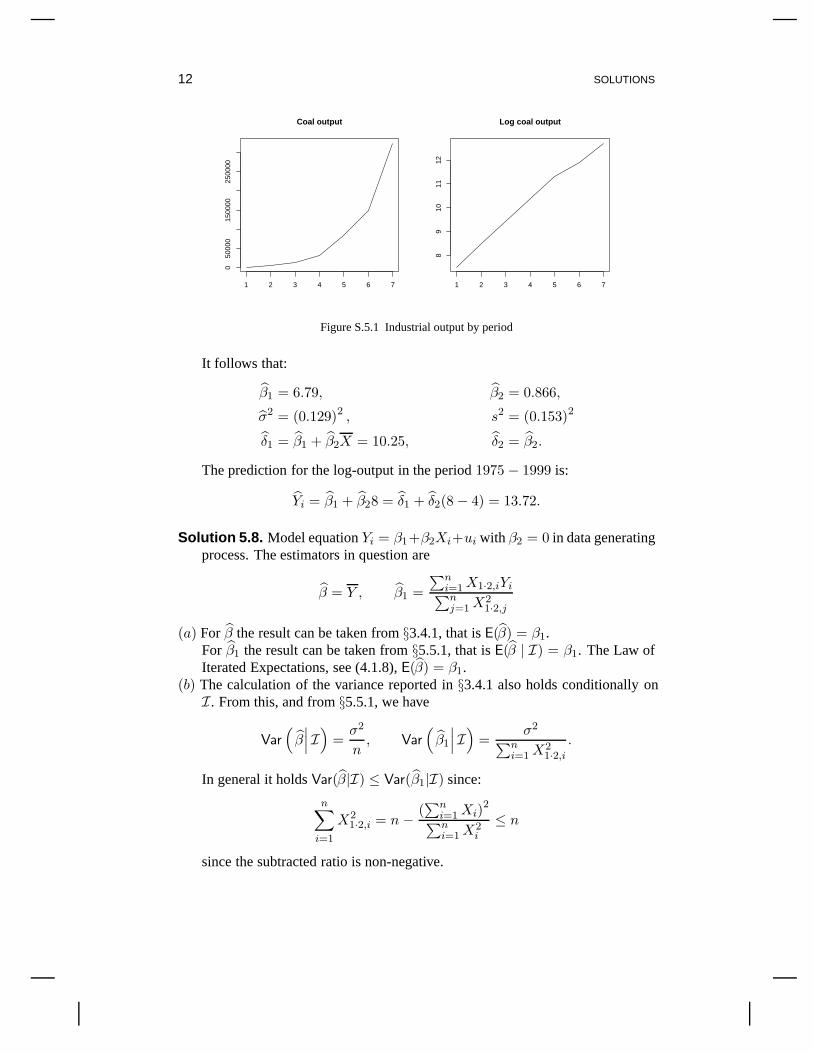
Solution 5.6.(a) See Figure S.5.1.(b) The following statistics have sufficient information about the data:

T∑t=1

Yt = 71.7424,T∑

t=1

Y 2t = 756.3848, T = 7,

T∑t=1

t = 28,T∑

t=1

t2 = 140,T∑

t=1

tYt = 311.2105.

12 SOLUTIONS

1 2 3 4 5 6 7

050

000

1500

0025

0000

Coal output

1 2 3 4 5 6 7

89

1011

12

Log coal output

Figure S.5.1 Industrial output by period

It follows that:

β1 = 6.79, β2 = 0.866,

σ2 = (0.129)2 , s2 = (0.153)2

δ1 = β1 + β2X = 10.25, δ2 = β2.

The prediction for the log-output in the period 1975 − 1999 is:

Yi = β1 + β28 = δ1 + δ2(8 − 4) = 13.72.

Solution 5.8. Model equation Yi = β1+β2Xi+ui with β2 = 0 in data generatingprocess. The estimators in question are

β = Y , β1 =∑n

i=1 X1·2,iYi∑nj=1 X2

1·2,j

(a) For β the result can be taken from §3.4.1, that is E(β) = β1.For β1 the result can be taken from §5.5.1, that is E(β | I) = β1. The Law ofIterated Expectations, see (4.1.8), E(β) = β1.

(b) The calculation of the variance reported in §3.4.1 also holds conditionally onI . From this, and from §5.5.1, we have

Var(

β∣∣∣ I) =

σ2

n, Var

(β1

∣∣∣ I) =σ2∑n

i=1 X21·2,i

.

In general it holds Var(β|I) ≤ Var(β1|I) since:

n∑i=1

X21·2,i = n − (

∑ni=1 Xi)

2∑ni=1 X2

i

≤ n

since the subtracted ratio is non-negative.

SOLUTIONS 13

(c) We have equality, Var(β|I) = Var(β1|I), when the numerator of the subtractedratio is zero, that is

∑ni=1 Xi = 0.

(d) The ratio of the variances is:

Var(

β1

∣∣∣ I)Var

(β∣∣∣ I) =

σ2∑ni=1 X2

1·2,i

/σ2

n=

{1 − (

∑ni=1 Xi)

2

n∑n

i=1 X2i

}−1

,

that is the inverse of one minus the square of a correlation type coefficientbased on the intercept X1,i and the regressor X2,i = Xi. It this correlationtype quantity is close to one the variance ratio is large. For instance, if it holdsthat X1 = · · · = Xm = M while Xm+1 = · · ·Xn = 0 the variance ratio is

Var(

β1

∣∣∣I)Var

(β∣∣∣I) =

{1 − (mM)2

nn(M2)

}−1

=(1 − m

n

)−1,

which is large if m is close to n. Note, that the actual value M of the regressorsdoes not matter in this particular calculation.

Solution 5.10. The results in (5.2.10) are:

Yi = δ1 + δ2X2·1,i,

where the estimators are:

δ1 = Y , δ2 =∑n

i=1 X2·1,i(Yi − Y )∑nj=1 X2

2·1,j

.

It follows from this that:

Yi − Yi = Yi − δ1 − δ2X2·1,i = Yi − Y − δ2X2·1,i,

Yi − Y = δ1 + δ2X2·1,i − Y = δ2X2·1,i.

The sum of cross products of these terms are:

n∑i=1

(Yi − Yi

)(Yi − Y

)=

n∑i=1

(Yi − Y − δ2X2·1,i

)(δ2X2·1,i

)= δ2

{n∑

i=1

(Yi − Y

)X2·1,i − δ2

n∑i=1

X22·1,i

}.

It follows from the above definition of δ2 that the expression in curly bracketsis zero.

14 SOLUTIONS

Solution 5.12.(a) First, show the identity for the variance estimators. From §5.4.3 it follows that

n(σ2

R − σ2)=

n∑i=1

(Yi − Y

)2 {1 − (1 − r2)}

= r2n∑

i=1

(Yi − Y

)2=

{∑ni=1 X2·1,i

(Yi − Y

)}2∑ni=1 X2

2·1,i

= β22

n∑i=1

X22·1,i.

Secondly, using that F = Z2 and the expression for se(β2) and for s2 stated in§5.5.3 it holds:

F = Z2 =β2

2{se(β2)

}2

=β2

2

∑ni=1 X2

2·1,i

s2=

β22

∑ni=1 X2

2·1,i

σ2n/(n − 2)

Insert the above expression for the variance terms to get:

F =n(σ2

R − σ2)

σ2n/(n − 2)=

(σ2

R − σ2)

σ2/(n − 2).

(b) For the second expression extend the fraction by 1/σ2R and use (5.4.6) to get:

F =

(σ2

R − σ2)

σ2/(n − 2)=

(1 − σ2/σ2

R

)σ2/σ2

R/(n − 2)=

r2

(1 − r2)/(n − 2).

For the third expression use (5.4.10):

F =r2

(1 − r2)/(n − 2)=

ESS/TSS

(RSS/TSS)/(n − 2)=

ESS

RSS/(n − 2).

Solution 5.14. To get r2 we can use the formula r2 = (σ2R − σ2)/σ2

R. Here:

σ2R = n−1

n∑i=1

(Yi − Y )2 = n−1n∑

i=1

Y 2i − Y

2

= (756.3848/7) − (71.7424/7)2 = 3.014727.

Therefore:

r2 =3.014727 − (0.129)2

3.014727= 0.99448.

The test statistics are:

F =r2/1

(1 − r2)/(7 − 2)= 900.7971, Z =

√F = 30.01.

SOLUTIONS 15

The tests are:One-sided t-test: reject since 30.01 > 2.02. (95% quantile of t[5] is 2.02)Two sided t-test: reject since |30.01| > 2.57. (97.5% quantile of t[5] is 2.57)F-test: reject since 901 > 6.61. (95% quantile of f[1, 5] is 6.61)

Chapter SixThe matrix algebra of two-variable regression

Solution 6.2.(a) First multiply matrices:

X′X=(

1 1 1 11 −1 1 −1

)⎛⎜⎜⎝1 11 −11 11 −1

⎞⎟⎟⎠ =(

4 00 4

)

X′Y =(

1 1 1 11 −1 1 −1

)⎛⎜⎜⎝1234

⎞⎟⎟⎠ =(

10−2

).

Then find the inverse of X′X. This is a diagonal matrix so the inverse is simplythe inverse of the diagonal elements:

(X′X

)−1 =(

1/4 00 1/4

).

Then multiply matrices to get the least squares estimator:

(X′X

)−1 X′Y =(

1/4 00 1/4

)(10−2

)=(

10/4−2/4

)=(

5/2−1/2

).

(b) The matrix multiplication “X′Y(X′X)−1” makes no sense, since X′Y is a(2 × 1)-matrix, while X′X is a (2 × 2)-matrix, so the column-dimension ofX′Y is one, while the row-dimension of X′Y is two.

The matrix multiplication “X′YX′X

” is not well-defined. Even if X′Y and X′Xhad the same dimension it is not clear whether it would mean multiplying X′Yfrom the left by the inverse of X′X, or from the right by the inverse of X′X,or dividing each of the elements of X′Y by the respective elements of X′X.In general, these operations would give different results.

Solution 6.4.(a) The inverse of a (2 × 2)-matrix can be found using the formula (6.2.1). Thus,

16 SOLUTIONS

the inverse of the matrix X′X in (6.3.3) it then:

(X′X

)−1 =( ∑n

i=1 12∑n

i=1 Xi∑ni=1 Xi

∑ni=1 X2

i

)−1

=1

det (X′X)

( ∑ni=1 X2

i −∑ni=1 Xi

−∑ni=1 Xi

∑ni=1 12

),

where det(X′X) is the determinant of X′X given by:

det(X′X

)=

(n∑

i=1

12

)(n∑

i=1

X2i

)−(

n∑i=1

Xi

)2

.

The least squares estimator is then

β =1

det (X′X)

( ∑ni=1 X2

i −∑ni=1 Xi

−∑ni=1 Xi

∑ni=1 12

)( ∑ni=1 Yi∑ni=1 XiYi

)=

1det (X′X)

( ∑ni=1 X2

i

∑ni=1 Yi −

∑ni=1 Xi

∑ni=1 XiYi∑n

i=1 12∑n

i=1 XiYi −∑n

i=1 Xi∑n

i=1 Yi

).

(b) The expressions in (5.2.1) arise by simplification of the above expression. Con-sider initially the second element and divide numerator and denominator by∑n

i=1 12 = n:

β2 =

(∑ni=1 12

∑ni=1 XiYi −

∑ni=1 Xi

∑ni=1 Yi

)/n{

(∑n

i=1 12)(∑n

i=1 X2i

)− (∑n

i=1 Xi)2}

/n

=∑n

i=1 XiYi − (∑n

i=1 Xi/n)∑n

i=1 Yi∑ni=1 X2

i − n (∑n

i=1 Xi/n)2.

=∑n

i=1 XiYi − X∑n

i=1 Yi∑ni=1 X2

i − n(X)2 .

Due to the formula found in Exercise 5.5(b) this reduces to the desired expres-sion:

β2 =∑n

i=1 Yi

(Xi − X

)∑ni=1

(Xi − X

)2 .

Consider now the first element and divide both numerator and denominator by

SOLUTIONS 17∑ni=1 12 = n:

β1 =

(∑ni=1 X2

i

∑ni=1 Yi −

∑ni=1 Xi

∑ni=1 XiYi

)/n{

(∑n

i=1 12)(∑n

i=1 X2i

)− (∑n

i=1 Xi)2}

/n

=∑n

i=1 X2i (∑n

i=1 Yi/n) − (∑n

i=1 Xi/n)∑n

i=1 XiYi∑ni=1 X2

i − n (∑n

i=1 Xi/n)2.

=∑n

i=1 X2i Y − X

∑ni=1 XiYi∑n

i=1 X2i − n

(X)2 .

Now, add and subtract nX2Y to get:

β1 =

(∑ni=1 X2

i − nX2)

Y − X(∑n

i=1 XiYinXY)

∑ni=1 X2

i − n(X)2 .

Due to the formula found in Exercise 5.5(b) this reduces to the desired expres-sion:

β1 = Y − β2X.

Solution 6.6.(a) When Yi

D= N[β, σ2] then:

Y =

⎛⎜⎝ Y1...

Yn

⎞⎟⎠ , X =

⎛⎜⎝ 1...1

⎞⎟⎠ .

By matrix multiplication:

X′Y =n∑

i=1

Yi = nY , X′X =n∑

i=1

1 = n,(X′X

)−1 =1n

,

so that:

β =(X′X

)−1 X′Y = Y .

(b) When YiD= N[βXi, σ

2] then:

Y =

⎛⎜⎝ Y1...

Yn

⎞⎟⎠ , X =

⎛⎜⎝ X1...

Xn

⎞⎟⎠ .

By matrix multiplication:

X′Y =n∑

i=1

XiYi, X′X =n∑

i=1

X2i ,

(X′X

)−1 =

(n∑

i=1

X2i

)−1

,

18 SOLUTIONS

so that:

β =∑n

i=1 XiYi∑ni=1 X2

i

.

(c) When YiD= N[β1 + β2Xi, σ

2] then:

Y =

⎛⎜⎝ Y1...

Yn

⎞⎟⎠ , X =

⎛⎜⎝ 1 X1...

...1 Xn

⎞⎟⎠ .

By matrix multiplication:

X′Y =( ∑n

i=1 Yi∑ni=1 XiYi

),

X′X=(

n∑n

i=1 Xi∑ni=1 Xi

∑ni=1 X2

i

),

(X′X

)−1 =1

det (X′X)

( ∑ni=1 X2

i −∑ni=1 Xi

−∑ni=1 Xi n

),

where det(X′X) = n∑n

i=1 X2i − (

∑ni=1 Xi)2, so that:

β =1

det (X′X)

( ∑ni=1 X2

i

∑ni=1 Yi −

∑ni=1 Xi

∑ni=1 YiXi

n∑n

i=1 YiXi −∑n

i=1 Xi∑n

i=1 Yi

).

By Exercise 6.4(b) this reduces further to the expressions in (5.2.1).

(d) When YiD= N[β1 + β2Xi, σ

2] with∑n

i=1 Xi = 0 the expressions in (c) reduceto:

Y =

⎛⎜⎝ Y1...

Yn

⎞⎟⎠ , X =

⎛⎜⎝ 1 X1...

...1 Xn

⎞⎟⎠ .

By matrix multiplication:

X′Y =( ∑n

i=1 Yi∑ni=1 XiYi

),

X′X=(

n 00∑n

i=1 X2i

),

(X′X

)−1 =1

det (X′X)

( ∑ni=1 X2

i 00 n

)=

(1n 00 1∑n

i=1 X2i

),

where det(X′X) = n∑n

i=1 X2i , so that:

β =

⎛⎝ 1n

∑ni=1 Yi∑n

i=1 YiXi∑ni=1 X2

i

⎞⎠ .

SOLUTIONS 19

Note, that unlike in (c) this result is a combination of the results in (a) and (b).

Chapter SevenThe multiple regression model

Solution 7.2. The calculations in this exercise are somewhat long. They could bereduced by using matrix algebra as set out in Chapter 8.

(a) The formula (7.2.8) gives:

δ2 = β2 + aβ3, δ3 = β3, so β2 = δ2 − aδ3.

Inserting the expression for a in (7.2.6) and forδ2 and δ3 in (7.2.12) then resultsin:

β2 =∑n

i=1 YiX2·1,i∑nj=1 X2

2·1,j

−(∑n

j=1 X3·1,jX2·1,j∑nk=1 X2

2·1,k

)∑ni=1 YiX3·1,2,i∑nj=1 X2

3·1,2,j

.

Put these expressions into a common fraction:

β2 =

∑ni=1 YiX2·1,i

⎧⎪⎨⎪⎩∑nj=1 X2

3·1,j −(∑n

j=1 X2·1,jX3·1,j

)2

∑nj=1 X2

2·1,j

⎫⎪⎬⎪⎭∑nj=1 X2

2·1,j

∑nj=1 X2

3·1,j −(∑n

j=1 X2·1,jX3·1,j

)2

−∑n

j=1 X2·1,jX3·1,j∑n

i=1 YiX3·1,i∑nj=1 X2

2·1,j

∑nj=1 X2

3·1,j −(∑n

j=1 X2·1,jX3·1,j

)2

+

∑ni=1 YiX2·1,i

(∑nj=1 X2·1,jX3·1,j

)2

∑nj=1 X2

2·1,j∑nj=1 X2

2·1,j

∑nj=1 X2

3·1,j −(∑n

j=1 X2·1,jX3·1,j

)2 ,

which reduces to:

β2 =

∑ni=1 YiX2·1,i

∑nj=1 X2

3·1,j −∑n

j=1 X2·1,jX3·1,j∑n

i=1 YiX3·1,i∑nj=1 X2

2·1,j

∑nj=1 X2

3·1,j −(∑n

j=1 X2·1,jX3·1,j

)2 .

Divide through by∑n

j=1 X23·1,j to see that:

β2 =∑n

i=1 YiX2·1,3,i∑nj=1 X2

2·1,3,j

.

20 SOLUTIONS

(b) The formula (7.2.8) gives:

β1 = δ1 − δ2X2 − δ3

(X3 − aX2

).

Start by rewriting the first two components:

δ1 − δ2X2 =

∑nj=1 X1,jYj∑n

j=1 X21,j

−∑n

j=1 X2·1,jYj∑nj=1 X2

2·1,j

(∑nj=1 X1,jX2,j∑n

j=1 X21,j

).

Bring them on a common fraction as:

δ1 − δ2X2 =

∑nj=1 X1,jYj

∑nj=1 X2

2·1,j −∑n

j=1 X2·1,jYj∑n

j=1 X1,jX2,j∑nj=1 X2

1,j

∑nj=1 X2

2·1,j

.

Divide numerator and denominator by∑n

j=1 X22,j to get:

δ1 − δ2X2 =

∑nj=1 X1,jYj

{1 − (

∑nj=1 X1,jX2,j)2∑n

j=1 X21,j

∑nj=1 X2

2,j

}∑n

j=1 X21·2,j

−

(∑nj=1 X2,jYj −

∑nj=1 X2,jX1,j

∑nj=1 X1,jYj∑n

j=1 X21,j

) ∑nj=1 X1,jX2,j∑n

j=1 X22,j∑n

j=1 X21·2,j

=

∑nj=1 X1·2,jYj∑nj=1 X2

1·2,j

.

Continue by analysing the third component the third component in the sameway. This is:

δ3

(X3 − aX2

)= δ3

{∑nj=1 X1,jX3,j∑n

j=1 X21,j

−(∑n

j=1 X3·1,jX2·1,j∑nj=1 X2

2·1,j

)∑nj=1 X1,jX2,j∑n

j=1 X21,j

}

Bring this on a common fraction:

δ3

(X3 − aX2

)=

δ3∑nj=1 X2

1,j

∑nj=1 X2

2·1,j

⎡⎢⎣ n∑j=1

X1,jX3,j

⎧⎪⎨⎪⎩n∑

j=1

X22,j −

(∑nj=1 X1,jX2,j

)2

∑nj=1 X2

1,j

⎫⎪⎬⎪⎭−⎛⎝ n∑

j=1

X3,jX2,j −∑n

j=1 X3,jX1,j∑n

j=1 X1,jX2,j∑nj=1 X2

1,j

⎞⎠∑nj=1 X1,jX2,j∑n

j=1 X22,j

⎤⎦ .

SOLUTIONS 21

Divide numerator and denominator by∑n

j=1 X22,j to get:

δ3

(X3 − aX2

)= δ3

∑nj=1 X3·2,jX1·2,j∑n

j=1 X21·2,j

.

Now bring all the components together:

β1 =

∑nj=1 X1·2,jYj∑nj=1 X2

1·2,j

−∑n

j=1 X3·1,2,jYj∑nj=1 X2

3·1,2,j

(∑nj=1 X3·2,jX1·2,j∑n

j=1 X21·2,j

.

).

As before, bring these on a common fraction. Then divide numerator anddenominator by

∑nj=1 X2

3·2,j to get the desired expression:

β1 =

∑nj=1 X1·2,3,jYj∑n

j=1 X21·2,3,j

.

Solution 7.4. The residuals from the two-variable model are given in (5.2.11) as:

Yi = (Yi − Y ) − γY (X2,i − X2),

X3,i = (X3,i − X3) − γX(X2,i − X2),

where γY and γX are the least squares estimators:

γY =∑n

i=1(Yi − Y )(X2,i − X2)∑ni=1(X2,i − X2)2

,

γX =∑n

i=1(X3,i − X3)(X2,i − X2)∑ni=1(X2,i − X2)2

.

The least-squares estimator from the regression of Yi on X3,i is

γ = [ one variable model ] =∑n

i=1 YiX3,i∑ni=1 X2

3,i

= [ see below ] =∑n

i=1 YiX3·1,2,i∑ni=1 X2

3·1,2,i

.

The denominator is:n∑

i=1

X23,i =

n∑i=1

{(X3,i − X3) − γX(X2,i − X2)}2

=n∑

i=1

(X3,i − X3)2 − {∑ni=1(X3,i − X3)(X2,i − X2)}2∑n

i=1(X2,i − X2)2

=n∑

i=1

X23·1,2,i.

22 SOLUTIONS

The numerator is:

n∑i=1

YiX3,i

=n∑

i=1

{(Yi − Y ) − γY (X2,i − X2)}{(X3,i − X3) − γX(X2,i − X2)}

=n∑

i=1

(Yi − Y )(X3,i − X3)

−∑n

i=1(Yi − Y )(X2,i − X2)∑n

i=1(X3,i − X3)(X2,i − X2)∑ni=1(X2,i − X2)2

=n∑

i=1

YiX3·1,2,i.

Solution 7.6. The idea is to show that:

n∑i=1

u2y·1,2,i = (1 − r2

y,2·1)n∑

i=1

(Yi − Y )2,

n∑i=1

u23·1,2,i = (1 − r2

3,2·1)n∑

i=1

(X3,i − X3)2,

n∑i=1

uy·1,2,iu3·1,2,i = (ry,3·1 − ry,2·1r2,3·1)

×{

n∑i=1

(Yi − Y )2n∑

i=1

(X3,i − X3)2}1/2

.

The desired expression then arise by dividing the latter expression with thesquare root of the two first. The first two expressions are proved as following.From the two-variable regression analysis of Yi on X1,i = 1,X2,i it is found

SOLUTIONS 23

that:

n∑i=1

u2y·1,2,i

=n∑

i=1

{(Yi − Y ) −

∑nj=1(Yi − Y )(X2,j − X2)∑n

j=1(X2,j − X2)2(X2,j − X2)

}2

=n∑

i=1

(Yi − Y )2 − {∑nj=1(Yi − Y )(X2,j − X)}2∑n

j=1(X2,j − X2)2

=n∑

i=1

(Yi − Y )2[1 − {∑n

j=1(Yi − Y )(X2,j − X2)}2∑ni=1(Yi − Y )2

∑nj=1(X2,j − X2)2

]

=(1 − r2

y,2·1) n∑

i=1

(Yi − Y )2.

as desired. The last expression is proved in the same way:

n∑i=1

uy·1,2,iu3·1,2,i

=n∑

i=1

{(Yi − Y ) −

∑nj=1(Yi − Y )(X2,j − X2)∑n

j=1(X2,j − X2)2(X2,i − X2)

}

×{

(X3,i − X3) −∑n

j=1(X3,j − X3)(X2,j − X2)∑nj=1(X2,j − X2)2

(X2,i − X2)

}

=n∑

i=1

(Yi − Y )(X3,i − X3)

−{∑nj=1(Yj − Y )(X2,j − X2)}{

∑nj=1(X3,j − X3)(X2,j − X2)}∑n

j=1(X2,j − X2)2

= (ry,3·1 − ry,2·1r2,3·1)

{n∑

i=1

(Yi − Y )2n∑

i=1

(X3,i − X3)2}1/2

.

Solution 7.8.(a) The formula (7.4.1) gives:

R2 =ESS

TSS=∑n

i=1(Yi − Y )2∑ni=1(Yi − Y )2

.

Noting that δ1 = Y then apply (7.2.15) to the numerator, and note that thedenominator is the sum of squared residuals in a regression of Yi on a constant.

24 SOLUTIONS

Thus:

R2 =δ22

∑ni=1 X2

2·1,i + δ23

∑ni=1 X2

3·1,2,i∑ni=1 u2

y·1.

(b) The same argument as in (a), but for a two-variable regression, where R2 equalsr2y·2,1 So for the numerator apply (5.2.10) instead of (7.2.15).

(c) From the definition in §7.3.1 we have:

r2y,2·1,2

n∑i=1

u2y·1,2,i =

(∑n

i=1 uy·1,2,iu3·2,1,i)2∑n

i=1 u23·1,2,i

.

But;∑n

i=1 uy·1,2,iu3·2,1,i =∑n

i=1 yiu3·2,1,i and u3·1,2,i = X3·1,2,i so:

r2y,2·1,2

n∑i=1

u2y·1,2,i =

(∑n

i=1 yiX3·2,1,i)2∑n

i=1 X23·1,2,i

= δ23

n∑i=1

X23·1,2,i,

which gives the desired formula.(d) This is the formula (5.4.10).(e) Use the results in the sequence (a), (b), (d), (c) to get:

1 − R2

= [ use (a) ] = 1 − δ22

∑ni=1 X2

2·1,i∑ni=1 u2

y·1− δ2

3

∑ni=1 X2

3·1,2,i∑ni=1 u2

y·1

= [ use (b) ] = 1 − r2y,2·1 −

δ23

∑ni=1 X2

3·1,2,i∑ni=1 u2

y·1

= [ extend fraction ] = 1 − r2y,2·1 −

(δ23

∑ni=1 X2

3·1,2,i∑ni=1 u2

y·1,2

)(∑ni=1 u2

y·1,2∑ni=1 u2

y·1

)

= [ use (d) ] =(1 − r2

y,2·1)(

1 − δ23

∑ni=1 X2

3·1,2,i∑ni=1 u2

y·1,2

)= [ use (c) ] =

(1 − r2

y,2·1) (

1 − r2y,3·2,1.

)Solution 7.10. From (7.6.2) with RSSR = TSS, m = 2, k = 3 it follows:

F =(TSS − RSS) /2

RSS/(n − 3).

Exploiting the relation (7.4.4) that TSS = ESS + RSS then gives:

F =ESS/2

(TSS − ESS) /(n − 3)=

(ESS/TSS) /2{1 − (ESS/TSS)} /(n − 3)

The desired expression then follows from (7.4.1).