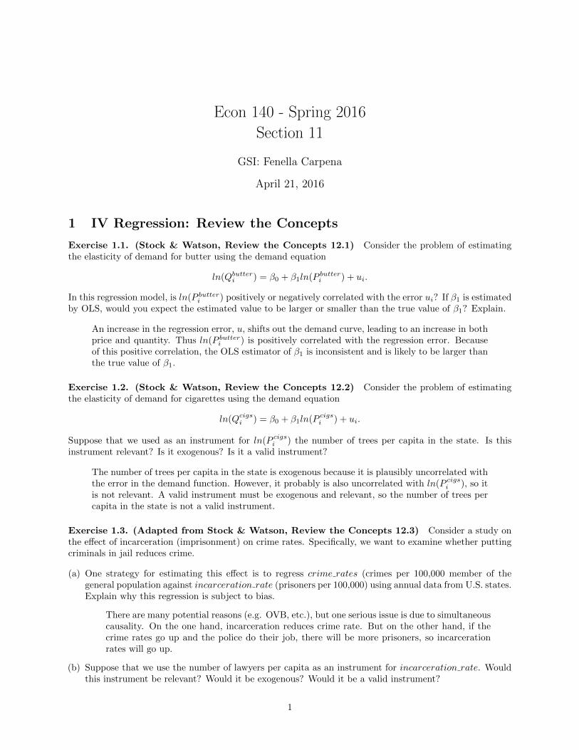
Econ 140 - Spring 2016

Section 11

GSI: Fenella Carpena

April 21, 2016

1 IV Regression: Review the Concepts

Exercise 1.1. (Stock & Watson, Review the Concepts 12.1) Consider the problem of estimatingthe elasticity of demand for butter using the demand equation

ln(Qbutteri ) = β0 + β1ln(P butter

i ) + ui.

In this regression model, is ln(P butteri ) positively or negatively correlated with the error ui? If β1 is estimated

by OLS, would you expect the estimated value to be larger or smaller than the true value of β1? Explain.

An increase in the regression error, u, shifts out the demand curve, leading to an increase in bothprice and quantity. Thus ln(P butter

i ) is positively correlated with the regression error. Becauseof this positive correlation, the OLS estimator of β1 is inconsistent and is likely to be larger thanthe true value of β1.

Exercise 1.2. (Stock & Watson, Review the Concepts 12.2) Consider the problem of estimatingthe elasticity of demand for cigarettes using the demand equation

ln(Qcigsi ) = β0 + β1ln(P cigs

i ) + ui.

Suppose that we used as an instrument for ln(P cigsi ) the number of trees per capita in the state. Is this

instrument relevant? Is it exogenous? Is it a valid instrument?

The number of trees per capita in the state is exogenous because it is plausibly uncorrelated withthe error in the demand function. However, it probably is also uncorrelated with ln(P cigs

i ), so itis not relevant. A valid instrument must be exogenous and relevant, so the number of trees percapita in the state is not a valid instrument.

Exercise 1.3. (Adapted from Stock & Watson, Review the Concepts 12.3) Consider a study onthe effect of incarceration (imprisonment) on crime rates. Specifically, we want to examine whether puttingcriminals in jail reduces crime.

(a) One strategy for estimating this effect is to regress crime rates (crimes per 100,000 member of thegeneral population against incarceration rate (prisoners per 100,000) using annual data from U.S. states.Explain why this regression is subject to bias.

There are many potential reasons (e.g. OVB, etc.), but one serious issue is due to simultaneouscausality. On the one hand, incarceration reduces crime rate. But on the other hand, if thecrime rates go up and the police do their job, there will be more prisoners, so incarcerationrates will go up.

(b) Suppose that we use the number of lawyers per capita as an instrument for incarceration rate. Wouldthis instrument be relevant? Would it be exogenous? Would it be a valid instrument?

1

The number of lawyers is arguably correlated with the incarceration rate, so it is relevant(although this should be checked in the data as well, using the methods in Section 12.3).However, states with higher than expected crime rates (with positive regression errors) arelikely to have more lawyers (criminals must be defended and prosecuted), so the number oflawyers will be positively correlated with the regression error. This means that the number oflawyers is not exogenous. A valid instrument must be exogenous and relevant, so the numberof lawyers is not a valid instrument.

Exercise 1.4. (Adapted from Stock & Watson, Review the Concepts 12.4) Does a new medicalprocedure (in this example, cardiac catheterization) prolong lives?

(a) Suppose we answer the above question by comparing patients who received the treatment to those whodid not. This leads to regressing the length of survival of the patient, months survived, on a binaryvariable for whether the patient received the procedure, got treatment. Explain why this regression issubject to bias.

There is sample selection bias the doctor and the patient decide to undertake the new procedure(e.g., they decide to do it if they believe it might be effective). If the healthiest patients arethe ones who receive the treatment, then the OLS estimate will be biased and will appearmore effective than it really is.

(b) Suppose that we use as an instrument for got treatment, the difference between the distance from thepatient’s home to the nearest cardiac catheterization hospital, and the distance to the nearest hospitalof any sort (which did not offer the treatment); this instrument takes on the value zero if the nearesthospital is a cardiac catheterization hospital, and otherwise it is positive. How could you determinewhether this instrument is relevant? How could you determine whether this instrument is exogenous?

If the difference in distance is a valid instrument, then it must be correlated with X, which inthis case is a binary variable indicating whether the patient received cardiac catheterization.Instrument relevance can be checked by regressing got treatment on “difference in distance.”In this regression, if the F -stat testing that the coefficient on the “difference in distance”variable is less than 10, then the instrument is weak. Checking instrument exogeneity is moredifficult. If there are more instruments than endogenous regressors, then joint exogeneity of theinstruments can be tested using the J-test. However, if the number of instruments is equal tothe number of endogenous regressors, then it is impossible to test for exogeneity statistically. Inthis case, we have one endogenous regressor (got treatment) and one instrument (difference indistance), so the J-test cannot be used. Expert judgment is required to assess the exogeneity.

Exercise 1.5. (Stock & Watson, Exercise 12.7) In an IV regression model with one regressor, Xi,and two instruments, Z1i and Z2i, the value of the J-statistic is J = 18.2.

(a) Does this suggest that E(ui|Z1i, Z2i) 6= 0? Explain.

Yes. Under the null hypothesis of instrument exogeneity, the J statistic is distributed as aχ22−1 random variable, with a 1% critical value of 6.63. Thus we reject the null, the statistic

is significant, and instrument exogeneity E(ui|Z1i, Z2i) = 0 is rejected.

(b) Does this suggest that E(ui|Z1i) 6= 0? Explain.

No. The J test suggests that E(ui|Z1i, Z2i) 6= 0, but doesn’t provide evidence about whetherthe problem is with Z1i or Z2i (or both).

2

Exercise 1.6. (Stock & Watson, Exercise 12.9) A researcher is interested in the effect of militaryservice on human capital. He collects data from a random sample of 4000 workers aged 40 and runs the OLSregression Yi = β0 + β1Xi + ui, where Yi is the worker i’s annual earnings and Xi is a binary variable thatis equal to 1 if the person served in the military and 0 otherwise.

(a) Explain why the OLS estimates are likely to unreliable. (Hint: Which variables are omitted from theregression? Are they correlated with military service?)

There are other factors that could affect both the choice to serve in the military and annualearnings. One example could be education, although this could be included in the regression asa control variable. Another variable is ability which is difficult to measure, and thus difficultto control for in the regression.

(b) During the Vietnam War there was a draft, where priority for the draft was determined by a nationallottery. (The days of the year were randomly reordered 1 through 365. Those with birthdates orderedfirst were drafted before those with birthdates ordered second, and so forth.) Explain how the lotterymight be used as an instrument to estimate the effect of military service on earnings.

The draft was determined by a national lottery so the choice of serving in the military wasrandom. Because it was randomly selected, the lottery number is uncorrelated with individualcharacteristics that may affect earning and hence the instrument is exogenous. Because itaffected the probability of serving in the military, the lottery number is relevant.

2 IV Regression: Stata Example

Exercise 2.1. (Adapted from Stock & Watson, Empirical Exercise 12.1) In this exercise, we willuse Stata to estimate the effect of fertility on women’s labor supply. The data set fertility.dta containsinformation on married women aged 21-35 with two or more children. The variables we will use are:

• weeksworked: mom’s weeks worked in 1979

• morekids: dummy variable equal to 1 if mom had more than 2 kids

• twoboys: dummy variable equal to 1 if mom’s first two kids are boys

• twogirls: dummy variable equal to 1 if mom’s first two kids are girls

• age: age of mom at 1980 census

Using these data, we are interested in understanding the following question: how much does a woman’s laborsupply fall when she has an additional child? Hence, the regression we want to estimate is:

weeksworked = β0 + β1morekids+ β2age+ u

(a) Using Stata, implement an IV regression of weeksworked on morekids and age, and using twoboys andtwogirls as instruments for morekids, by estimating each of the two stages using OLS. What are Y ,W , X, and Z here?

The Y variable is weeksworked, W is age, X is morekids, and we have two instruments Z1

and Z2 for twoboys and twogirls, respectively. The commands for each stage are as follows:

• First stage: reg morekids twoboys twogirls age, robust

• Obtain predicted values for endogenous variable: predict morekids hat, xb

• Second stage: reg weeksworked morekids hat age, robust

3

. reg morekids twoboys twogirls age, robust

Linear regression Number of obs = 254654

F( 3,254650) = 1342.66

Prob > F = 0.0000

R-squared = 0.0151

Root MSE = .48185

------------------------------------------------------------------------------

| Robust

morekids | Coef. Std. Err. t P>|t| [95% Conf. Interval]

-------------+----------------------------------------------------------------

twoboys | .0578227 .0023012 25.13 0.000 .0533124 .0623329

twogirls | .0789634 .0023967 32.95 0.000 .0742659 .0836608

age | .0143633 .0002769 51.88 0.000 .0138206 .014906

_cons | -.0902769 .0084654 -10.66 0.000 -.1068689 -.073685

------------------------------------------------------------------------------

. predict morekids_hat, xb

. reg weeksworked morekids_hat age, robust

Linear regression Number of obs = 254654

F( 2,254651) = 1729.59

Prob > F = 0.0000

R-squared = 0.0124

Root MSE = 21.731

------------------------------------------------------------------------------

| Robust

weeksworked | Coef. Std. Err. t P>|t| [95% Conf. Interval]

-------------+----------------------------------------------------------------

morekids_hat | -5.58984 1.239716 -4.51 0.000 -8.01965 -3.160029

age | .7977256 .0215668 36.99 0.000 .7554553 .8399959

_cons | -3.099863 .3770051 -8.22 0.000 -3.838783 -2.360943

------------------------------------------------------------------------------

(b) Perform the same IV regression as in part (a) but using Stata’s ivregress command. Verify that thecoefficients are the same you obtained are the same as in part (a), but the standard errors are different;why is this the case?

. ivregress 2sls weeksworked (morekids = twoboys twogirls) age, robust

Instrumental variables (2SLS) regression Number of obs = 254654

Wald chi2(2) = 3518.15

Prob > chi2 = 0.0000

R-squared = 0.0295

Root MSE = 21.542

------------------------------------------------------------------------------

| Robust

weeksworked | Coef. Std. Err. z P>|z| [95% Conf. Interval]

-------------+----------------------------------------------------------------

morekids | -5.58984 1.229054 -4.55 0.000 -7.998741 -3.180938

age | .7977256 .0213784 37.31 0.000 .7558246 .8396265

4

_cons | -3.099863 .373689 -8.30 0.000 -3.83228 -2.367446

------------------------------------------------------------------------------

Instrumented: morekids

Instruments: age twoboys twogirls

Comparing the results we have here to those in part (a), we find that the coefficients are thesame but the standard errors are different. The standard errors in part (a) are not correctbecause it does not take into account the fact that the regressor morekids hat used in thesecond stage is coming from a first stage regression (so it is a random variable, because ofsampling variability). In contrast, the ivregress 2sls does take it into account, so thestandard errors from this command are correct.

(c) For the Stata command in part (b):

(i) Explain each part of this Stata command.

ivregress 2sls tells Stata to run a two-stage least-squares regression. Then, ivregress2sls is followed by the outcome variable Y , which in this case is weeksworked. In the partwhere we have (morekids = twoboys twogirls), this says that the endogenous variableX is morekids, and twoboys, twogirls are the two instruments Z1 and Z2, respectively.Finally, age is a control variable here, which corresponds with W in our notation.

Note that when executing the code in part (b), the first stage regression is not shownin the Stata output. However if we wanted Stata to show the output for the first stage,we just need to add the word first at the end of the command, i.e., ivregress 2sls

weeksworked (morekids = twoboys twogirls) age, robust first. Executing this com-mand in Stata will show the following output, which includes the results from the first stageregression before showing the second stage results:

. ivregress 2sls weeksworked (morekids = twoboys twogirls) age, robust first

First-stage regressions

-----------------------

Number of obs = 254654

F( 3, 254650) = 1342.66

Prob > F = 0.0000

R-squared = 0.0151

Adj R-squared = 0.0151

Root MSE = 0.4819

------------------------------------------------------------------------------

| Robust

morekids | Coef. Std. Err. t P>|t| [95% Conf. Interval]

-------------+----------------------------------------------------------------

age | .0143633 .0002769 51.88 0.000 .0138206 .014906

twoboys | .0578227 .0023012 25.13 0.000 .0533124 .0623329

twogirls | .0789634 .0023967 32.95 0.000 .0742659 .0836608

_cons | -.0902769 .0084654 -10.66 0.000 -.1068689 -.073685

------------------------------------------------------------------------------

Instrumental variables (2SLS) regression Number of obs = 254654

Wald chi2(2) = 3518.15

Prob > chi2 = 0.0000

R-squared = 0.0295

Root MSE = 21.542

5

------------------------------------------------------------------------------

| Robust

weeksworked | Coef. Std. Err. z P>|z| [95% Conf. Interval]

-------------+----------------------------------------------------------------

morekids | -5.58984 1.229054 -4.55 0.000 -7.998741 -3.180938

age | .7977256 .0213784 37.31 0.000 .7558246 .8396265

_cons | -3.099863 .373689 -8.30 0.000 -3.83228 -2.367446

------------------------------------------------------------------------------

Instrumented: morekids

Instruments: age twoboys twogirls

(ii) How many instruments do we have? How many endogenous regressors? Is the regression overiden-tified, underidentified, or exactly indentified?

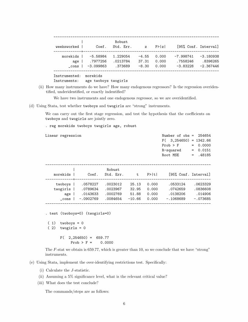
We have two instruments and one endogenous regressor, so we are overidentified.

(d) Using Stata, test whether twoboys and twogirls are “strong” instruments.

We can carry out the first stage regression, and test the hypothesis that the coefficients ontwoboys and twogirls are jointly zero.

. reg morekids twoboys twogirls age, robust

Linear regression Number of obs = 254654

F( 3,254650) = 1342.66

Prob > F = 0.0000

R-squared = 0.0151

Root MSE = .48185

------------------------------------------------------------------------------

| Robust

morekids | Coef. Std. Err. t P>|t| [95% Conf. Interval]

-------------+----------------------------------------------------------------

twoboys | .0578227 .0023012 25.13 0.000 .0533124 .0623329

twogirls | .0789634 .0023967 32.95 0.000 .0742659 .0836608

age | .0143633 .0002769 51.88 0.000 .0138206 .014906

_cons | -.0902769 .0084654 -10.66 0.000 -.1068689 -.073685

------------------------------------------------------------------------------

. test (twoboys=0) (twogirls=0)

( 1) twoboys = 0

( 2) twogirls = 0

F( 2,254650) = 659.77

Prob > F = 0.0000

The F -stat we obtain is 659.77, which is greater than 10, so we conclude that we have “strong”instruments.

(e) Using Stata, implement the over-identifying restrictions test. Specifically:

(i) Calculate the J-statistic.

(ii) Assuming a 5% significance level, what is the relevant critical value?

(iii) What does the test conclude?

The commands/steps are as follows:

6

• Step 1: Estimate IV 2SLS regression: ivregress 2sls weeksworked (morekids = twoboys

twogirls) age, robust

• Step 2: Obtain residuals: predict uhat, resid

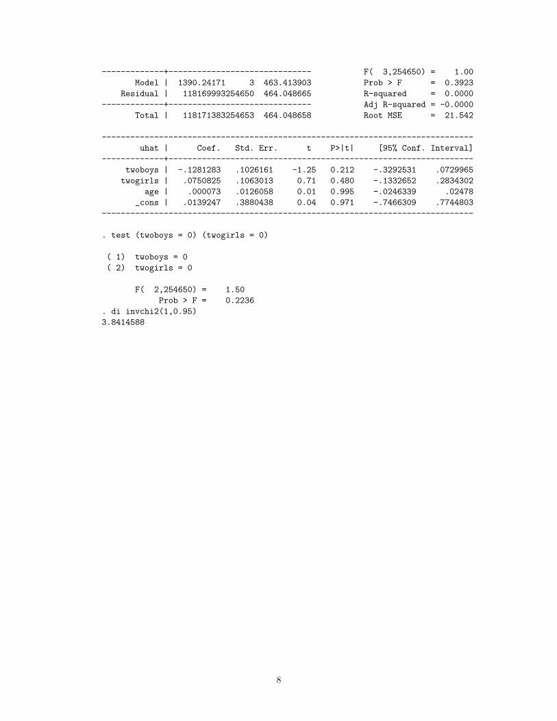
• Step 3: Regress residuals on Z’s and W ’s using homoskedastic errors: reg uhat twoboys

twogirls age

• Step 4: Test the hypothesis that the coefficients on Z’s are jointly zero and obtain ho-moskedastic F -stat: test (twoboys = 0) (twogirls = 0). Doing this in Stata (seeoutput below), we obtain the F -stat = 1.50.

• Step 5: Calculate J-stat = m · F where m is the number of instruments. In this case,m = 2 so our J-stat = 2 ∗ 1.50 = 3.00.

• Step 6: Find the critical value from the Chi-squared distribution with m − k degrees offreedom (where m is again the number of instruments Z, and k is the number of endoge-nous variables X). In this example, m − k = 2 − 1 = 1. Using the Chi-squared table atthe back of the textbook and 5% significance, we find that the critical value is 3.84.

Instead of using the Chi-squared table to find this critical value, we also could have usedthe Stata command di invchi2(1,0.95) where di means display, the first number insidethe parenthesis is the degrees of freedom, i.e., m− k = 1, and the second number 0.95 isbecause we are using α = 0.05, so that 1− α = 0.95.

• Step 7: Conclusion: If J-stat > critical value, we reject H0, which is evidence that atleast one of the Z’s is not exogenous. If J-stat < critical value, we fail to reject H0,which is evidence that the Z’s are exogenous. In our example, we fail to reject H0 because3.00 < 3.84.

. ivregress 2sls weeksworked (morekids = twoboys twogirls) age, robust

Instrumental variables (2SLS) regression Number of obs = 254654

Wald chi2(2) = 3518.15

Prob > chi2 = 0.0000

R-squared = 0.0295

Root MSE = 21.542

------------------------------------------------------------------------------

| Robust

weeksworked | Coef. Std. Err. z P>|z| [95% Conf. Interval]

-------------+----------------------------------------------------------------

morekids | -5.58984 1.229054 -4.55 0.000 -7.998741 -3.180938

age | .7977256 .0213784 37.31 0.000 .7558246 .8396265

_cons | -3.099863 .373689 -8.30 0.000 -3.83228 -2.367446

------------------------------------------------------------------------------

Instrumented: morekids

Instruments: age twoboys twogirls

. predict uhat, resid

. reg uhat twoboys twogirls age

Source | SS df MS Number of obs = 254654

7

-------------+------------------------------ F( 3,254650) = 1.00

Model | 1390.24171 3 463.413903 Prob > F = 0.3923

Residual | 118169993254650 464.048665 R-squared = 0.0000

-------------+------------------------------ Adj R-squared = -0.0000

Total | 118171383254653 464.048658 Root MSE = 21.542

------------------------------------------------------------------------------

uhat | Coef. Std. Err. t P>|t| [95% Conf. Interval]

-------------+----------------------------------------------------------------

twoboys | -.1281283 .1026161 -1.25 0.212 -.3292531 .0729965

twogirls | .0750825 .1063013 0.71 0.480 -.1332652 .2834302

age | .000073 .0126058 0.01 0.995 -.0246339 .02478

_cons | .0139247 .3880438 0.04 0.971 -.7466309 .7744803

------------------------------------------------------------------------------

. test (twoboys = 0) (twogirls = 0)

( 1) twoboys = 0

( 2) twogirls = 0

F( 2,254650) = 1.50

Prob > F = 0.2236

. di invchi2(1,0.95)

3.8414588

8

3 Final Exam Review: Spring 2014 Final, Question 4

In honor of Mother’s Day last weekend, this question concerns a dataset consisting of more than a quarter of a million moms between the ages of 21 and 35 drawn from the 1980 Census. We focus on five variables in that dataset:

A labor economist is interested in answering how the number of children affects mothers’ labor supply decisions, and specifically whether there is a causal effect of the dummy indicator morekids on weeksworked . The researcher’s population regression is: . Below you will find the log of a series of Stata program commands executed on this dataset by the researcher, and below that is a list of questions to be answered using this output.

. summ weeksworked morekids samesex hispan age Variable | Obs Mean Std. Dev. Min Max -------------+-------------------------------------------------------- weeksworked | 254654 19.01833 21.86728 0 52 morekids | 254654 .3805634 .4855263 0 1 samesex | 254654 .5055683 .49997 0 1 hispan | 254654 .0742066 .2621073 0 1 age | 254654 30.39327 3.386447 21 35 . correlate weeksworked morekids samesex hispan age (obs=254654) | weeksw~d morekids samesex hispan age -------------+--------------------------------------------- weeksworked | 1.0000 morekids | -0.1196 1.0000 samesex | -0.0097 0.0695 1.0000 hispan | -0.0104 0.0777 -0.0002 1.0000 age | 0.1111 0.0999 -0.0031 -0.0657 1.0000 . regress weeksworked morekids age , robust Linear regression Number of obs = 254654 F( 2,254651) = 4252.27 Prob > F = 0.0000 R-squared = 0.0296 Root MSE = 21.541 ------------------------------------------------------------------------------ | Robust weeksworked | Coef. Std. Err. t P>|t| [95% Conf. Interval] -------------+---------------------------------------------------------------- morekids | -5.946385 .0865748 -68.68 0.000 -6.11607 -5.776701 age | .8028323 .0121562 66.04 0.000 .7790064 .8266582 _cons | -3.119385 .3674612 -8.49 0.000 -3.839599 -2.399171 ------------------------------------------------------------------------------ . regress morekids samesex hispan , robust Linear regression Number of obs = 254654 F( 2,254651) = 1368.81 Prob > F = 0.0000 R-squared = 0.0109 Root MSE = .48288 ------------------------------------------------------------------------------ | Robust morekids | Coef. Std. Err. t P>|t| [95% Conf. Interval] -------------+---------------------------------------------------------------- samesex | .0675405 .0019132 35.30 0.000 .0637907 .0712902 hispan | .1439261 .0037629 38.25 0.000 .136551 .1513013 _cons | .3357368 .0013596 246.93 0.000 .333072 .3384017 ------------------------------------------------------------------------------ . test samesex hispan ( 1) samesex = 0 ( 2) hispan = 0 F( 2,254651) = 1368.81

Variable Description weeksworked number of weeks worked by the mom in 1979 morekids = 1 if mom had more than 2 children samesex = 1 if 2 or more children and first two are same sexhispan = 1 if mom is Hispanic age age of mom in the 1980 census

9

Prob > F = 0.0000 . ivregress 2sls weeksworked (morekids = samesex) age , robust Instrumental variables (2SLS) regression Number of obs = 254654 Wald chi2(2) = 3520.60 Prob > chi2 = 0.0000 R-squared = 0.0296 Root MSE = 21.541 ------------------------------------------------------------------------------ | Robust weeksworked | Coef. Std. Err. z P>|z| [95% Conf. Interval] -------------+---------------------------------------------------------------- morekids | -6.06062 1.258803 -4.81 0.000 -8.527828 -3.593413 age | .8044685 .0217279 37.02 0.000 .7618825 .8470544 _cons | -3.125639 .3739658 -8.36 0.000 -3.858599 -2.39268 ------------------------------------------------------------------------------ Instrumented: morekids Instruments: age samesex . ivregress 2sls weeksworked (morekids = hispan) age , robust Instrumental variables (2SLS) regression Number of obs = 254654 Wald chi2(2) = 3469.70 Prob > chi2 = 0.0000 R-squared = 0.0205 Root MSE = 21.642 ------------------------------------------------------------------------------ | Robust weeksworked | Coef. Std. Err. z P>|z| [95% Conf. Interval] -------------+---------------------------------------------------------------- morekids | -1.63085 1.037662 -1.57 0.116 -3.66463 .4029299 age | .7410219 .0192269 38.54 0.000 .7033379 .7787059 _cons | -2.8831 .3736879 -7.72 0.000 -3.615515 -2.150685 ------------------------------------------------------------------------------ Instrumented: morekids Instruments: age hispan . ivregress 2sls weeksworked (morekids = samesex hispan) age , robust Instrumental variables (2SLS) regression Number of obs = 254654 Wald chi2(2) = 3506.36 Prob > chi2 = 0.0000 R-squared = 0.0265 Root MSE = 21.575 ------------------------------------------------------------------------------ | Robust weeksworked | Coef. Std. Err. z P>|z| [95% Conf. Interval] -------------+---------------------------------------------------------------- morekids | -3.430894 .7992682 -4.29 0.000 -4.997431 -1.864357 age | .7668035 .0166953 45.93 0.000 .7340813 .7995257 _cons | -2.981656 .3707483 -8.04 0.000 -3.70831 -2.255003 ------------------------------------------------------------------------------ Instrumented: morekids Instruments: age samesex hispan . predict u2slshat , resid . regress u2slshat samesex hispan age Source | SS df MS Number of obs = 254654 -------------+------------------------------ F( 3,254650) = 2.44 Model | 3410.54014 3 1136.84671 Prob > F = 0.0622 Residual | 118536486254650 465.487869 R-squared = 0.0000 -------------+------------------------------ Adj R-squared = 0.0000 Total | 118539896254653 465.495778 Root MSE = 21.575 ------------------------------------------------------------------------------ u2slshat | Coef. Std. Err. t P>|t| [95% Conf. Interval] -------------+---------------------------------------------------------------- samesex | -.1783145 .0855142 -2.09 0.037 -.34592 -.0107091 hispan | .2819951 .1634709 1.73 0.085 -.0384035 .6023937 age | .0013517 .0126525 0.11 0.915 -.0234469 .0261504 _cons | .0281409 .3904391 0.07 0.943 -.7371093 .7933912 ------------------------------------------------------------------------------ . test samesex hispan ( 1) samesex = 0 ( 2) hispan = 0 F( 2,254650) = 3.66 Prob > F = 0.0256

10

Economics 140 Page 6 Final Exam

. predict u2slshat , resid . regress u2slshat samesex hispan age Source | SS df MS Number of obs = 254654 -------------+------------------------------ F( 3,254650) = 2.44 Model | 3410.54014 3 1136.84671 Prob > F = 0.0622 Residual | 118536486254650 465.487869 R-squared = 0.0000 -------------+------------------------------ Adj R-squared = 0.0000 Total | 118539896254653 465.495778 Root MSE = 21.575 ------------------------------------------------------------------------------ u2slshat | Coef. Std. Err. t P>|t| [95% Conf. Interval] -------------+---------------------------------------------------------------- samesex | -.1783145 .0855142 -2.09 0.037 -.34592 -.0107091 hispan | .2819951 .1634709 1.73 0.085 -.0384035 .6023937 age | .0013517 .0126525 0.11 0.915 -.0234469 .0261504 _cons | .0281409 .3904391 0.07 0.943 -.7371093 .7933912 ------------------------------------------------------------------------------ . test samesex hispan ( 1) samesex = 0 ( 2) hispan = 0 F( 2,254650) = 3.66 Prob > F = 0.0256

a) [5] Why did the researcher include the age of the mother in the OLS regression? What would you expect

would happen to the coefficient on morekids if age was excluded? Answer: The age of the mother should correlate with her employability within the 21-35 range, but also with the number of kids she has had. Leaving it out will cause omitted variable bias. The OLSE would be biased upward assuming that older moms tend to have more kids than younger ones.

b) [4] Give one reason why you would suspect that the coefficient on morekids would not be unbiased and consistent estimate of the population coefficient. Answer: One reason is that there is simultaneous causality occurring, with more weeks worked resulting in more income which, in turn, makes more kids affordable for the mother and her family. There could be omitted variable that affects both amount of work and number of kids. For example, mother’s education level is omitted from the regression. Education level likely is positively related to employment opportunities and it is also known that the number of children is inversely related to education of the mother.

c) [4] What is the interpretation of the coefficient on morekids in the OLS regression. Is it economically significant? Is it statistically significant? Answer: A mother who has more than 2 kids works 5.95 fewer weeks on average compared to a mother who has just 1 or 2 kids. The average number of weeks worked is 19 so a change of 6 is quite economically significant. A t stat of 68 ensures it is strongly different from zero. From the above output, the researcher thinks that two of the other variables in the dataset, samesex and hispan , are potential instruments for morekids. The variable samesex takes the value of 1 when the mother has had 2 or more children and the first two were both boys or both girls, and 0 otherwise.

d) [5] Why might the variable samesex be a “relevant” instrument for the endogenous regressor morekids? Explain why there is empirical evidence in the Stata output supporting the relevance of both samesex and hispan. Answer: samesex is relevant if it is statistically correlated with morekids. If, after having two children of the same sex, mothers and parents wish to have a third child in the hopes they will have a child of the other gender, then morekids and samesex will be positively correlated. The correlation matrix offers a bit of evidence that this is so. Also the test of whether both instruments are jointly zero in the first stage regression yields an F = 1,368 far in excess of the rule of thumb of 10.

Economics 140 Page 7 Final Exam

e) [4] Assuming that both candidates are valid instruments, why does the researcher have a case of “over identification”? What evidence do you see in the Stata output that confirms that there is an issue with overidentification? Answer: There are two instruments but only one endogenous regressor: m – k = 2 – 1 = 1 degree of over identification. Inspection of the two TSLS regression results using the two candidates separately yields quite different coefficient estimates: -6.06 and -1.63 using samesex and hispan as instruments, respectively. These estimates are sufficiently different from one another to call into question exogeneity of one or both instruments.

f) [4] For these variables, what does it mean for the candidate instruments to meet the second criterion of a valid instrument, i.e., to be “exogenous”? What is in the Stata output that should make you suspicious that the one or the other or both of these candidate instruments are not exogenous? Answer: An instrument is “exogenous” if it is uncorrelated with the error term from the population regression. As in part (e) the TSLS estimates of coefficient on morekids differs depending on the instrument chose: -6.06 vs. -1.63.

g) [7] How did the researcher attempt to determine whether the candidate instruments are exogenous? What should the researcher conclude? Answer: The researcher has estimated the J statistic to perform a test of over identifying restrictions. First she performed TSLS, then found the residuals evaluated at the original values of the regressor (not first stage fitted values), then performed homoskedasticity-only regression of those residuals on the two instruments and the control. The J = mF where F is the F stat testing whether coefficients on the two instruments are jointly zero. The J stat is asymptotically Chi Squared with 1 degree of freedom. Here F = 3.66 so J = 7.32, and so is much larger than the critical value of 3.84 at the 5% significance level that is found in the first row of Table 3.

11