ECE276B: Planning & Learning in RoboticsLecture 3: The Dynamic Programming Algorithm

Lecturer:Nikolay Atanasov: natanasov@ucsd.edu

Teaching Assistants:Tianyu Wang: tiw161@eng.ucsd.eduYongxi Lu: yol070@eng.ucsd.edu

1

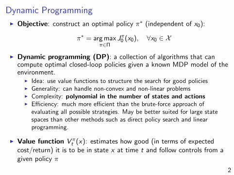
Dynamic Programming

I Objective: construct an optimal policy π∗ (independent of x0):

π∗ = arg maxπ∈Π

Jπ0 (x0), ∀x0 ∈ X

I Dynamic programming (DP): a collection of algorithms that cancompute optimal closed-loop policies given a known MDP model of theenvironment.

I Idea: use value functions to structure the search for good policiesI Generality: can handle non-convex and non-linear problemsI Complexity: polynomial in the number of states and actionsI Efficiency: much more efficient than the brute-force approach of

evaluating all possible strategies. May be better suited for large statespaces than other methods such as direct policy search and linearprogramming.

I Value function V πt (x): estimates how good (in terms of expected

cost/return) it is to be in state x at time t and follow controls from agiven policy π

2

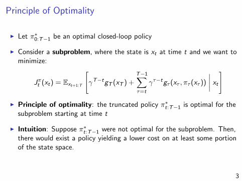
Principle of Optimality

I Let π∗0:T−1 be an optimal closed-loop policy

I Consider a subproblem, where the state is xt at time t and we want tominimize:

Jπt (xt) = Ext+1:T

[γT−tgT (xT ) +

T−1∑τ=t

γτ−tgτ (xτ , πτ (xτ ))

∣∣∣∣ xt]

I Principle of optimality: the truncated policy π∗t:T−1 is optimal for thesubproblem starting at time t

I Intuition: Suppose π∗t:T−1 were not optimal for the subproblem. Then,there would exist a policy yielding a lower cost on at least some portionof the state space.

3

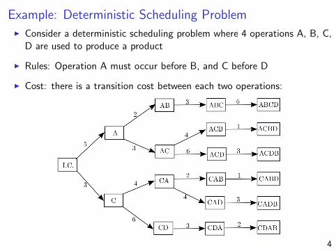
Example: Deterministic Scheduling ProblemI Consider a deterministic scheduling problem where 4 operations A, B, C,

D are used to produce a product

I Rules: Operation A must occur before B, and C before D

I Cost: there is a transition cost between each two operations:

4

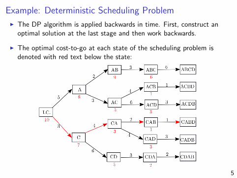
Example: Deterministic Scheduling Problem

I The DP algorithm is applied backwards in time. First, construct anoptimal solution at the last stage and then work backwards.

I The optimal cost-to-go at each state of the scheduling problem isdenoted with red text below the state:

5

The Dynamic Programming Algorithm

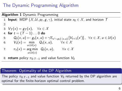
Algorithm 1 Dynamic Programming

1: Input: MDP (X ,U , pf , g , γ), initial state x0 ∈ X , and horizon T2:

3: VT (x) = gT (x), ∀x ∈ X4: for t = (T − 1) . . . 0 do5: Qt(x , u)← gt(x , u) + γEx ′∼pf (·|x ,u) [Vt+1(x ′)] , ∀x ∈ X , u ∈ U(x)6: Vt(x) = min

u∈U(x)Qt(x , u), ∀x ∈ X

7: πt(x) = arg minu∈U(x)

Qt(x , u), ∀x ∈ X

8: return policy π0:T−1 and value function V0

Theorem: Optimality of the DP Algorithm

The policy π0:T−1 and value function V0 returned by the DP algorithm areoptimal for the finite-horizon optimal control problem.

6

The Dynamic Programming Algorithm

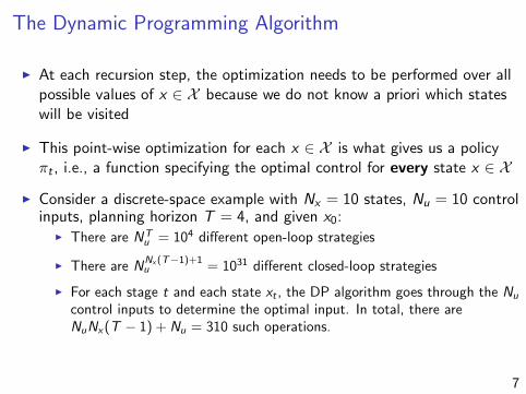
I At each recursion step, the optimization needs to be performed over allpossible values of x ∈ X because we do not know a priori which stateswill be visited

I This point-wise optimization for each x ∈ X is what gives us a policyπt , i.e., a function specifying the optimal control for every state x ∈ X

I Consider a discrete-space example with Nx = 10 states, Nu = 10 controlinputs, planning horizon T = 4, and given x0:

I There are NTu = 104 different open-loop strategies

I There are NNx (T−1)+1u = 1031 different closed-loop strategies

I For each stage t and each state xt , the DP algorithm goes through the Nu

control inputs to determine the optimal input. In total, there areNuNx(T − 1) + Nu = 310 such operations.

7

Proof of Dynamic Programming Optimality

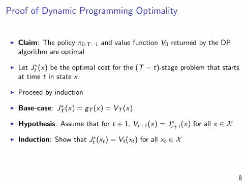
I Claim: The policy π0:T−1 and value function V0 returned by the DPalgorithm are optimal

I Let J∗t (x) be the optimal cost for the (T − t)-stage problem that startsat time t in state x .

I Proceed by induction

I Base-case: J∗T (x) = gT (x) = VT (x)

I Hypothesis: Assume that for t + 1, Vt+1(x) = J∗t+1(x) for all x ∈ X

I Induction: Show that J∗t (xt) = Vt(xt) for all xt ∈ X

8

Proof of Dynamic Programming Optimality

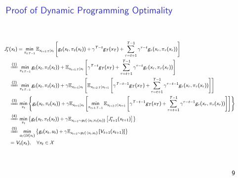
J∗t (xt) = minπt:T−1

Ext+1:T |xt

[gt(xt , πt(xt)) + γT−tgT (xT ) +

T−1∑τ=t+1

γτ−tgτ (xτ , πτ (xτ ))

](1)

=== minπt:T−1

gt(xt , πt(xt)) + Ext+1:T |xt

[γT−tgT (xT ) +

T−1∑τ=t+1

γτ−tgτ (xτ , πτ (xτ ))

](2)

=== minπt:T−1

gt(xt , πt(xt)) + γExt+1|xt

[Ext+2:T |xt+1

[γT−t−1gT (xT ) +

T−1∑τ=t+1

γτ−t−1gτ (xτ , πτ (xτ ))

]](3)

=== minπt

{gt(xt , πt(xt)) + γExt+1|xt

[min

πt+1:T−1

Ext+2:T |xt+1

[γT−t−1gT (xT ) +

T−1∑τ=t+1

γτ−t−1gτ (xτ , πτ (xτ ))

]]}(4)

=== minπt

{gt(xt , πt(xt)) + γExt+1∼pf (·|xt ,πt(xt))

[J∗t+1(xt+1)

]}(5)

=== minut∈U(xt)

{gt(xt , ut) + γExt+1∼pf (·|xt ,ut) [Vt+1(xt+1)]

}= Vt(xt), ∀xt ∈ X

9

Proof of Dynamic Programming Optimality

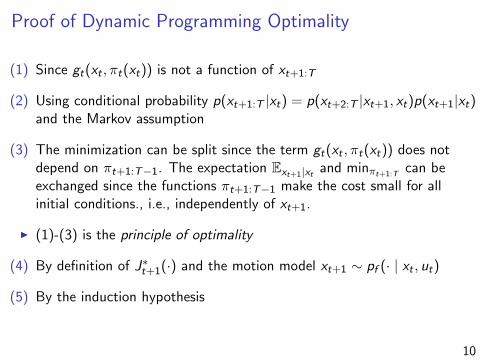
(1) Since gt(xt , πt(xt)) is not a function of xt+1:T

(2) Using conditional probability p(xt+1:T |xt) = p(xt+2:T |xt+1, xt)p(xt+1|xt)and the Markov assumption

(3) The minimization can be split since the term gt(xt , πt(xt)) does notdepend on πt+1:T−1. The expectation Ext+1|xt and minπt+1:T

can beexchanged since the functions πt+1:T−1 make the cost small for allinitial conditions., i.e., independently of xt+1.

I (1)-(3) is the principle of optimality

(4) By definition of J∗t+1(·) and the motion model xt+1 ∼ pf (· | xt , ut)

(5) By the induction hypothesis

10

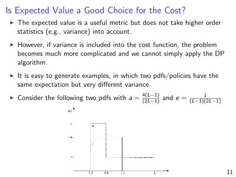
Is Expected Value a Good Choice for the Cost?I The expected value is a useful metric but does not take higher order

statistics (e.g., variance) into account.

I However, if variance is included into the cost function, the problembecomes much more complicated and we cannot simply apply the DPalgorithm.

I It is easy to generate examples, in which two pdfs/policies have thesame expectation but very different variance.

I Consider the following two pdfs with a = 4(L−1)(2L−1) and e = 1

(L−1)(2L−1)

11

Is Expected Value a Good Choice for the Cost?

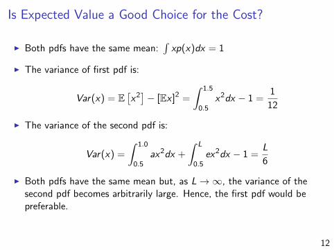
I Both pdfs have the same mean:∫xp(x)dx = 1

I The variance of first pdf is:

Var(x) = E[x2]− [Ex ]2 =

∫ 1.5

0.5x2dx − 1 =

1

12

I The variance of the second pdf is:

Var(x) =

∫ 1.0

0.5ax2dx +

∫ L

0.5ex2dx − 1 =

L

6

I Both pdfs have the same mean but, as L→∞, the variance of thesecond pdf becomes arbitrarily large. Hence, the first pdf would bepreferable.

12

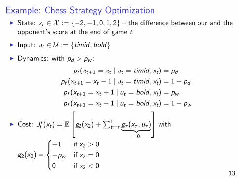
Example: Chess Strategy OptimizationI State: xt ∈ X := {−2,−1, 0, 1, 2} – the difference between our and the

opponent’s score at the end of game t

I Input: ut ∈ U := {timid , bold}

I Dynamics: with pd > pw :

pf (xt+1 = xt | ut = timid , xt) = pd

pf (xt+1 = xt − 1 | ut = timid , xt) = 1− pd

pf (xt+1 = xt + 1 | ut = bold , xt) = pw

pf (xt+1 = xt − 1 | ut = bold , xt) = 1− pw

I Cost: J∗t (xt) = E

g2(x2) +∑1

t=τ gτ (xτ , uτ )︸ ︷︷ ︸=0

with

g2(x2) =

−1 if x2 > 0

−pw if x2 = 0

0 if x2 < 013

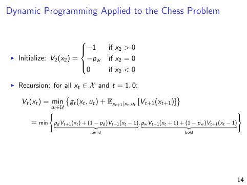
Dynamic Programming Applied to the Chess Problem

I Initialize: V2(x2) =

−1 if x2 > 0

−pw if x2 = 0

0 if x2 < 0

I Recursion: for all xt ∈ X and t = 1, 0:

Vt(xt) = minut∈U

{gt(xt , ut) + Ext+1|xt ,ut [Vt+1(xt+1)]

}= min

pdVt+1(xt) + (1− pd)Vt+1(xt − 1)︸ ︷︷ ︸timid

, pwVt+1(xt + 1) + (1− pw )Vt+1(xt − 1)︸ ︷︷ ︸bold

14

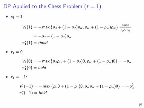
DP Applied to the Chess Problem (t = 1)

I x1 = 1:

V1(1) = −max {pd + (1− pd)pw , pw + (1− pw )pw}since

=====pd>pw

= −pd − (1− pd)pw

π∗1(1) = timid

I x1 = 0:

V1(0) = −max {pdpw + (1− pd)0, pw + (1− pw )0} = −pwπ∗1(0) = bold

I x1 = −1:

V1(−1) = −max {pd0 + (1− pd)0, pwpw + (1− pw )0} = −p2w

π∗1(−1) = bold

15

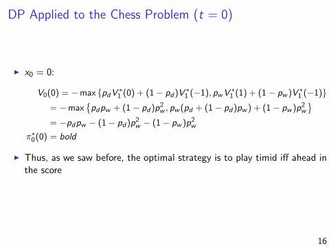
DP Applied to the Chess Problem (t = 0)

I x0 = 0:

V0(0) = −max {pdV ∗1 (0) + (1− pd)V ∗1 (−1), pwV∗1 (1) + (1− pw )V ∗1 (−1)}

= −max{pdpw + (1− pd)p2

w , pw (pd + (1− pd)pw ) + (1− pw )p2w

}= −pdpw − (1− pd)p2

w − (1− pw )p2w

π∗0(0) = bold

I Thus, as we saw before, the optimal strategy is to play timid iff ahead inthe score

16

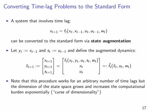
Converting Time-lag Problems to the Standard Form

I A system that involves time lag:

xt+1 = ft(xt , xt−1, ut , ut−1,wt)

can be converted to the standard form via state augmentation

I Let yt := xt−1 and st := ut−1 and define the augmented dynamics:

x̃t+1 :=

xt+1

yt+1

st+1

=

ft(xt , yt , ut , st ,wt)xtut

=: f̃t(x̃t , ut ,wt)

I Note that this procedure works for an arbitrary number of time lags butthe dimension of the state space grows and increases the computationalburden exponentially (“curse of dimensionality”)

17

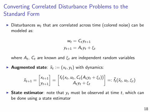
Converting Correlated Disturbance Problems to theStandard Form

I Disturbances wt that are correlated across time (colored noise) can bemodeled as:

wt = Ctyt+1

yt+1 = Atyt + ξt

where At , Ct are known and ξt are independent random variables

I Augmented state: x̃t := (xt , yt) with dynamics:

x̃t+1 =

[xt+1

yt+1

]=

[ft(xt , ut ,Ct(Atyt + ξt))

Atyt + ξt

]=: f̃t(x̃t , ut , ξt)

I State estimator: note that yt must be observed at time t, which canbe done using a state estimator

18