Dynkin systemFrom Wikipedia, the free encyclopedia

Contents

1 Dynkin system 11.1 Definitions . . . . . . . . . . . . . . . . . . . . . . . . . . . . . . . . . . . . . . . . . . . . . . 11.2 Dynkin’s π-λ theorem . . . . . . . . . . . . . . . . . . . . . . . . . . . . . . . . . . . . . . . . . 11.3 Notes . . . . . . . . . . . . . . . . . . . . . . . . . . . . . . . . . . . . . . . . . . . . . . . . . 21.4 References . . . . . . . . . . . . . . . . . . . . . . . . . . . . . . . . . . . . . . . . . . . . . . 2

2 Lebesgue measure 32.1 Definition . . . . . . . . . . . . . . . . . . . . . . . . . . . . . . . . . . . . . . . . . . . . . . . 3

2.1.1 Intuition . . . . . . . . . . . . . . . . . . . . . . . . . . . . . . . . . . . . . . . . . . . 32.2 Examples . . . . . . . . . . . . . . . . . . . . . . . . . . . . . . . . . . . . . . . . . . . . . . . 42.3 Properties . . . . . . . . . . . . . . . . . . . . . . . . . . . . . . . . . . . . . . . . . . . . . . . 42.4 Null sets . . . . . . . . . . . . . . . . . . . . . . . . . . . . . . . . . . . . . . . . . . . . . . . . 52.5 Construction of the Lebesgue measure . . . . . . . . . . . . . . . . . . . . . . . . . . . . . . . . 62.6 Relation to other measures . . . . . . . . . . . . . . . . . . . . . . . . . . . . . . . . . . . . . . 62.7 See also . . . . . . . . . . . . . . . . . . . . . . . . . . . . . . . . . . . . . . . . . . . . . . . . 62.8 References . . . . . . . . . . . . . . . . . . . . . . . . . . . . . . . . . . . . . . . . . . . . . . 7

3 Pi system 83.1 Examples . . . . . . . . . . . . . . . . . . . . . . . . . . . . . . . . . . . . . . . . . . . . . . . 83.2 Relationship to λ-Systems . . . . . . . . . . . . . . . . . . . . . . . . . . . . . . . . . . . . . . . 8

3.2.1 The π-λ Theorem . . . . . . . . . . . . . . . . . . . . . . . . . . . . . . . . . . . . . . . 93.3 π-Systems in Probability . . . . . . . . . . . . . . . . . . . . . . . . . . . . . . . . . . . . . . . 9

3.3.1 Equality in Distribution . . . . . . . . . . . . . . . . . . . . . . . . . . . . . . . . . . . . 103.3.2 Independent Random Variables . . . . . . . . . . . . . . . . . . . . . . . . . . . . . . . . 10

3.4 See also . . . . . . . . . . . . . . . . . . . . . . . . . . . . . . . . . . . . . . . . . . . . . . . . 113.5 Notes . . . . . . . . . . . . . . . . . . . . . . . . . . . . . . . . . . . . . . . . . . . . . . . . . 113.6 References . . . . . . . . . . . . . . . . . . . . . . . . . . . . . . . . . . . . . . . . . . . . . . 113.7 Text and image sources, contributors, and licenses . . . . . . . . . . . . . . . . . . . . . . . . . . 12

3.7.1 Text . . . . . . . . . . . . . . . . . . . . . . . . . . . . . . . . . . . . . . . . . . . . . . 123.7.2 Images . . . . . . . . . . . . . . . . . . . . . . . . . . . . . . . . . . . . . . . . . . . . 123.7.3 Content license . . . . . . . . . . . . . . . . . . . . . . . . . . . . . . . . . . . . . . . . 12

i

Chapter 1

Dynkin system

A Dynkin system, named after Eugene Dynkin, is a collection of subsets of another universal set Ω satisfying a setof axioms weaker than those of σ-algebra. Dynkin systems are sometimes referred to as λ-systems (Dynkin himselfused this term) or d-system.[1] These set families have applications in measure theory and probability.The primary relevance of λ-systems are their use in applications of the π-λ theorem.

1.1 Definitions

Let Ω be a nonempty set, and let D be a collection of subsets of Ω (i.e., D is a subset of the power set of Ω). ThenD is a Dynkin system if

1. Ω ∈ D ,

2. if A, B ∈ D and A ⊆ B, then B \ A ∈ D ,

3. if A1, A2, A3, ... is a sequence of subsets in D and An ⊆ An₊₁ for all n ≥ 1, then∪∞

n=1 An ∈ D .

Equivalently, D is a Dynkin system if

1. Ω ∈ D ,

2. if A ∈ D, then Ac ∈ D,

3. if A1, A2, A3, ... is a sequence of subsets in D such that Ai ∩ Aj = Ø for all i ≠ j, then∪∞

n=1 An ∈ D .

The second definition is generally preferred as it usually is easier to check.An important fact is that a Dynkin systemwhich is also a π-system (i.e., closed under finite intersection) is a σ-algebra.This can be verified by noting that condition 3 and closure under finite intersection implies closure under countableunions.Given any collection J of subsets of Ω , there exists a unique Dynkin system denotedDJ which is minimal withrespect to containing J . That is, if D is any Dynkin system containing J , then DJ ⊆ D . DJ is called theDynkin system generated by J . Note D∅ = ∅,Ω . For another example, let Ω = 1, 2, 3, 4 and J = 1 ;then DJ = ∅, 1, 2, 3, 4,Ω .

1.2 Dynkin’s π-λ theorem

If P is a π-system andD is a Dynkin system with P ⊆ D , then σP ⊆ D . In other words, the σ-algebra generatedby P is contained in D .One application of Dynkin’s π-λ theorem is the uniqueness of a measure that evaluates the length of an interval(known as the Lebesgue measure):

1

2 CHAPTER 1. DYNKIN SYSTEM

Let (Ω, B, λ) be the unit interval [0,1] with the Lebesgue measure on Borel sets. Let μ be another measure on Ωsatisfying μ[(a,b)] = b − a, and letD be the family of sets S such that μ[S] = λ[S]. Let I = (a,b),[a,b),(a,b],[a,b] : 0 <a ≤ b < 1 , and observe that I is closed under finite intersections, that I ⊂ D, and that B is the σ-algebra generated byI. It may be shown that D satisfies the above conditions for a Dynkin-system. From Dynkin’s π-λ Theorem it followsthat D in fact includes all of B, which is equivalent to showing that the Lebesgue measure is unique on B.Additional applications are in the article on π-systems.

1.3 Notes[1] Charalambos Aliprantis, Kim C. Border (2006). Infinite Dimensional Analysis: a Hitchhiker’s Guide, 3rd ed. Springer.

Retrieved August 23, 2010.

1.4 References• Gut, Allan (2005). Probability: A Graduate Course. New York: Springer. doi:10.1007/b138932. ISBN0-387-22833-0.

• Billingsley, Patrick (1995). Probability and Measure. New York: John Wiley & Sons, Inc. ISBN 0-471-00710-2.

• David Williams (2007). Probability with Martingales. Cambridge University Press. p. 193. ISBN 0-521-40605-6.

This article incorporates material from Dynkin system on PlanetMath, which is licensed under the Creative CommonsAttribution/Share-Alike License.

Chapter 2

Lebesgue measure

In measure theory, the Lebesgue measure, named after French mathematician Henri Lebesgue, is the standardway of assigning a measure to subsets of n-dimensional Euclidean space. For n = 1, 2, or 3, it coincides with thestandard measure of length, area, or volume. In general, it is also called n-dimensional volume, n-volume, or simplyvolume.[1] It is used throughout real analysis, in particular to define Lebesgue integration. Sets that can be assigneda Lebesgue measure are called Lebesgue measurable; the measure of the Lebesgue measurable set A is denoted byλ(A).Henri Lebesgue described this measure in the year 1901, followed the next year by his description of the Lebesgueintegral. Both were published as part of his dissertation in 1902.[2]

The Lebesgue measure is often denoted dx, but this should not be confused with the distinct notion of a volume form.

2.1 Definition

Given a subset E ⊆ R , with the length of an (open, closed, semi-open) interval I = [a, b] given by l(I) = b − a ,the Lebesgue outer measure λ∗(E) is defined as

λ∗(E) = inf ∞∑

k=1

l(Ik) : (Ik)k∈N with intervals open of sequence a is E ⊆∞∪k=1

Ik

The Lebesgue measure of E is given by its Lebesgue outer measure λ(E) = λ∗(E) if, for every A ⊆ R ,

λ∗(A) = λ∗(A ∩ E) + λ∗(A ∩ Ec)

2.1.1 Intuition

The first part of the definition states that the subsetE of the real numbers is reduced to its outer measure by coverageby sets of intervals. Each of these sets of intervals I covers E in the sense that when the intervals are combinedtogether by union, they contain E . The total length of any covering interval set can easily overestimate the measureof E , because E is a subset of the union of the intervals, and so the intervals may include points which are not in E. The Lebesgue outer measure emerges as the greatest lower bound (infimum) of the lengths from among all possiblesuch sets. Intuitively, it is the total length of those interval sets which fit E most tightly and do not overlap.That characterizes the Lebesgue outer measure. Whether this outer measure translates to the Lebesgue measureproper depends on an additional condition. This condition is tested by taking subsets of the real numbers A usingE as an instrument to split A into two partitions: the part of A which intersects with E and the remaining part ofA which is not in E : the set difference of A and E . These partitions of A are subject to the outer measure. If forall possible such subsets A of the real numbers, the partitions of A cut apart by E have outer measures which addup to the outer measure of A , then the outer Lebesgue measure of E gives its Lebesgue measure. Intuitively, this

3

4 CHAPTER 2. LEBESGUE MEASURE

condition means that the set E must not have some curious properties which causes a discrepancy in the measure ofanother set whenE is used as a “mask” to “clip” that set, hinting at the existence of sets for which the Lebesgue outermeasure does not give the Lebesgue measure. (Such sets are, in fact, not Lebesgue-measurable.)

2.2 Examples• Any closed interval [a, b] of real numbers is Lebesgue measurable, and its Lebesgue measure is the length b−a.The open interval (a, b) has the same measure, since the difference between the two sets consists only of theend points a and b and has measure zero.

• Any Cartesian product of intervals [a, b] and [c, d] is Lebesgue measurable, and its Lebesgue measure is(b−a)(d−c), the area of the corresponding rectangle.

• Moreover, every Borel set is Lebesgue measurable. However, there are Lebesgue measurable sets which arenot Borel sets.[3][4]

• Any countable set of real numbers has Lebesgue measure 0.

• In particular, the Lebesgue measure of the set of rational numbers is 0, although the set is dense in R.

• The Cantor set is an example of an uncountable set that has Lebesgue measure zero.

• Vitali sets are examples of sets that are not measurable with respect to the Lebesgue measure. Their existencerelies on the axiom of choice.

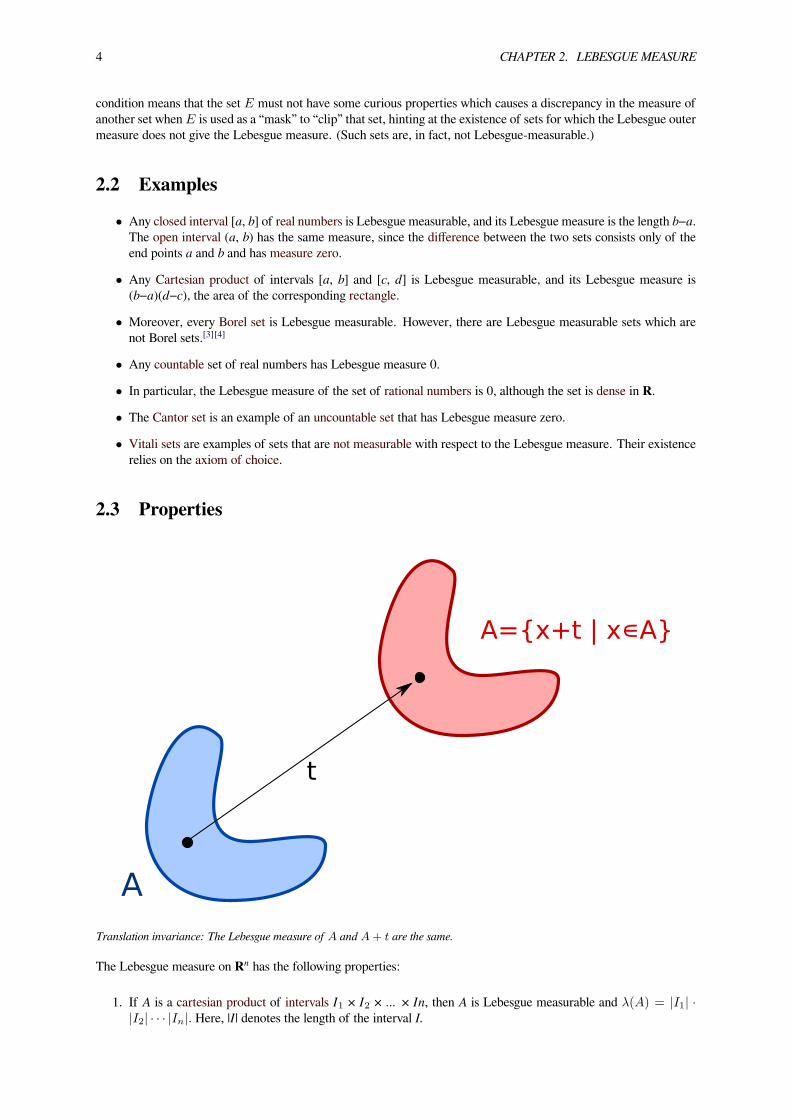
2.3 Properties

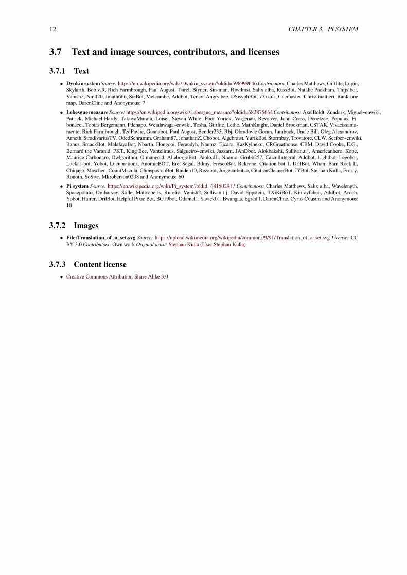
A

t

A=x+t | x∊A

Translation invariance: The Lebesgue measure of A and A+ t are the same.

The Lebesgue measure on Rn has the following properties:

1. If A is a cartesian product of intervals I1 × I2 × ... × In, then A is Lebesgue measurable and λ(A) = |I1| ·|I2| · · · |In|. Here, |I | denotes the length of the interval I.

2.4. NULL SETS 5

2. If A is a disjoint union of countably many disjoint Lebesgue measurable sets, then A is itself Lebesgue mea-surable and λ(A) is equal to the sum (or infinite series) of the measures of the involved measurable sets.

3. If A is Lebesgue measurable, then so is its complement.

4. λ(A) ≥ 0 for every Lebesgue measurable set A.

5. If A and B are Lebesgue measurable and A is a subset of B, then λ(A) ≤ λ(B). (A consequence of 2, 3 and 4.)

6. Countable unions and intersections of Lebesgue measurable sets are Lebesgue measurable. (Not a consequenceof 2 and 3, because a family of sets that is closed under complements and disjoint countable unions need notbe closed under countable unions: ∅, 1, 2, 3, 4, 1, 2, 3, 4, 1, 3, 2, 4 .)

7. If A is an open or closed subset of Rn (or even Borel set, see metric space), then A is Lebesgue measurable.

8. If A is a Lebesgue measurable set, then it is “approximately open” and “approximately closed” in the sense ofLebesgue measure (see the regularity theorem for Lebesgue measure).

9. A Lebesgue-measurable set can be “squeezed” between a containing open set and a contained closed set. I.e,if A is Lebesgue measurable then for every positive ε there exist an open set G and a closed set F such thatG⊇A⊇F and λ(G\A)<ε and λ(A\F)<ε.

10. A Lebesgue-measurable set can be “squeezed” between a containing Gδ set and a contained Fσ set. I.e, if Ais Lebesgue measurable then there exist a Gδ set G and an Fσ set F such that G⊇A⊇F and λ(G\A)=λ(A\F)=0.

11. Lebesgue measure is both locally finite and inner regular, and so it is a Radon measure.

12. Lebesgue measure is strictly positive on non-empty open sets, and so its support is the whole of Rn.

13. If A is a Lebesgue measurable set with λ(A) = 0 (a null set), then every subset of A is also a null set. A fortiori,every subset of A is measurable.

14. If A is Lebesgue measurable and x is an element of Rn, then the translation of A by x, defined by A + x = a+ x : a ∈ A, is also Lebesgue measurable and has the same measure as A.

15. If A is Lebesgue measurable and δ > 0 , then the dilation of A by δ defined by δA = δx : x ∈ A is alsoLebesgue measurable and has measure δnλ (A).

16. More generally, if T is a linear transformation and A is a measurable subset of Rn, then T(A) is also Lebesguemeasurable and has the measure | det(T )|λ (A) .

All the above may be succinctly summarized as follows:

The Lebesgue measurable sets form a σ-algebra containing all products of intervals, and λ is the uniquecomplete translation-invariant measure on that σ-algebra with λ([0, 1]× [0, 1]× · · · × [0, 1]) = 1.

The Lebesgue measure also has the property of being σ-finite.

2.4 Null sets

Main article: Null set

A subset of Rn is a null set if, for every ε > 0, it can be covered with countably many products of n intervals whosetotal volume is at most ε. All countable sets are null sets.If a subset of Rn has Hausdorff dimension less than n then it is a null set with respect to n-dimensional Lebesguemeasure. Here Hausdorff dimension is relative to the Euclidean metric on Rn (or any metric Lipschitz equivalent toit). On the other hand a set may have topological dimension less than n and have positive n-dimensional Lebesguemeasure. An example of this is the Smith–Volterra–Cantor set which has topological dimension 0 yet has positive1-dimensional Lebesgue measure.In order to show that a given set A is Lebesgue measurable, one usually tries to find a “nicer” set B which differs fromA only by a null set (in the sense that the symmetric difference (A − B) ∪ (B − A) is a null set) and then show that Bcan be generated using countable unions and intersections from open or closed sets.

6 CHAPTER 2. LEBESGUE MEASURE

2.5 Construction of the Lebesgue measure

Themodern construction of the Lebesgue measure is an application of Carathéodory’s extension theorem. It proceedsas follows.Fix n ∈ N. A box in Rn is a set of the form

B =n∏

i=1

[ai, bi] ,

where bi ≥ ai, and the product symbol here represents a Cartesian product. The volume of this box is defined to be

vol(B) =

n∏i=1

(bi − ai) .

For any subset A of Rn, we can define its outer measure λ*(A) by:

λ∗(A) = inf∑

B∈Cvol(B) : C covers union whose boxes of collection countable a is A

.

We then define the set A to be Lebesgue measurable if for every subset S of Rn,

λ∗(S) = λ∗(S ∩A) + λ∗(S \A) .

These Lebesgue measurable sets form a σ-algebra, and the Lebesgue measure is defined by λ(A) = λ*(A) for anyLebesgue measurable set A.The existence of sets that are not Lebesgue measurable is a consequence of a certain set-theoretical axiom, the axiomof choice, which is independent from many of the conventional systems of axioms for set theory. The Vitali theorem,which follows from the axiom, states that there exist subsets of R that are not Lebesgue measurable. Assuming theaxiom of choice, non-measurable sets with many surprising properties have been demonstrated, such as those of theBanach–Tarski paradox.In 1970, Robert M. Solovay showed that the existence of sets that are not Lebesgue measurable is not provable withinthe framework of Zermelo–Fraenkel set theory in the absence of the axiom of choice (see Solovay’s model).[5]

2.6 Relation to other measures

The Borel measure agrees with the Lebesgue measure on those sets for which it is defined; however, there are manymore Lebesgue-measurable sets than there are Borel measurable sets. The Borel measure is translation-invariant, butnot complete.The Haar measure can be defined on any locally compact group and is a generalization of the Lebesgue measure (Rn

with addition is a locally compact group).The Hausdorff measure is a generalization of the Lebesgue measure that is useful for measuring the subsets of Rn

of lower dimensions than n, like submanifolds, for example, surfaces or curves in R³ and fractal sets. The Hausdorffmeasure is not to be confused with the notion of Hausdorff dimension.It can be shown that there is no infinite-dimensional analogue of Lebesgue measure.

2.7 See also• Lebesgue’s density theorem

• Lebesgue measure of the set of Liouville numbers

2.8. REFERENCES 7

2.8 References[1] The term volume is also used, more strictly, as a synonym of 3-dimensional volume

[2] Henri Lebesgue (1902). “Intégrale, longueur, aire”. Université de Paris.

[3] Asaf Karagila. “What sets are Lebesgue measurable?". math stack exchange. Retrieved 26 September 2015.

[4] Asaf Karagila. “Is there a sigma-algebra on R strictly between the Borel and Lebesgue algebras?". math stack exchange.Retrieved 26 September 2015.

[5] Solovay, Robert M. (1970). “A model of set-theory in which every set of reals is Lebesgue measurable”. Annals ofMathematics. Second Series 92 (1): 1–56. doi:10.2307/1970696. JSTOR 1970696.

Chapter 3

Pi system

In mathematics, a π-system (or pi-system) on a set Ω is a collection P of certain subsets of Ω, such that

• P is non-empty.

• A ∩ B ∈ P whenever A and B are in P.

That is, P is a non-empty family of subsets of Ω that is closed under finite intersections. The importance of π-systemsarise from the fact that if two probability measures agree on a π-system, then they agree on the σ-algebra generatedby that π-system. Moreover, if other properties, such as equality of integrals, hold for the π-system, then they holdfor the generated σ-algebra as well. This is the case whenever the collection of subsets for which the property holdsis a λ-system. π-systems are also useful for checking independence of random variables.This is desirable because in practice, π-systems are often simpler to work with than σ-algebras. For example, it maybe awkward to work with σ-algebras generated by infinitely many sets σ(E1, E2, . . .) . So instead we may examinethe union of all σ-algebras generated by finitely many sets

∪n σ(E1, . . . , En) . This forms a π-system that generates

the desired σ-algebra. Another example is the collection of all interval subsets of the real line, along with the emptyset, which is a π-system that generates the very important Borel σ-algebra of subsets of the real line.

3.1 Examples

• ∀a, b ∈ R , the intervals (−∞, a] form a π-system, and the intervals (a, b] form a π-system, if the empty setis also included.

• The topology (collection of open subsets) of any topological space is a π-system.

• For any collection Σ of subsets of Ω, there exists a π-system IΣ which is the unique smallest π-system of Ω tocontain every element of Σ, and is called the π-system generated by Σ.

• For any measurable function f : Ω → R , the set If =f−1 ((−∞, x]) : x ∈ R

defines a π-system, and is

called the π-system generated by f. (Alternatively,f−1 ((a, b]) : a, b ∈ R, a < b

∪∅ defines a π-system

generated by f .)

• If P1 and P2 are π-systems for Ω1 and Ω2, respectively, then A1 × A2 : A1 ∈ P1, A2 ∈ P2 is a π-systemfor the product space Ω1×Ω2.

• Any σ-algebra is a π-system.

3.2 Relationship to λ-Systems

A λ-system on Ω is a set D of subsets of Ω, satisfying

8

3.3. Π-SYSTEMS IN PROBABILITY 9

• Ω ∈ D ,

• if A ∈ D then Ac ∈ D ,

• if A1, A2, A3, . . . is a sequence of disjoint subsets in D then ∪∞n=1An ∈ D .

Whilst it is true that any σ-algebra satisfies the properties of being both a π-system and a λ-system, it is not truethat any π-system is a λ-system, and moreover it is not true that any π-system is a σ-algebra. However, a usefulclassification is that any set system which is both a λ-system and a π-system is a σ-algebra. This is used as a step inproving the π-λ theorem.

3.2.1 The π-λ Theorem

Let D be a λ-system, and let I ⊆ D be a π-system contained in D . The π-λ Theorem[1] states that the σ-algebraσ(I) generated by I is contained in D : σ(I) ⊂ D .The π-λ theorem can be used to prove many elementary measure theoretic results. For instance, it is used in provingthe uniqueness claim of the Carathéodory extension theorem for σ-finite measures.[2]

The π-λ theorem is closely related to the monotone class theorem, which provides a similar relationship betweenmonotone classes and algebras, and can be used to derive many of the same results. Since π-systems are simplerclasses than algebras, it can be easier to identify the sets that are in them while, on the other hand, checking whetherthe property under consideration determines a λ-system is often relatively easy. Despite the difference between thetwo theorems, the π-λ theorem is sometimes referred to as the monotone class theorem.[1]

Example

Let μ₁ , μ2 : F → R be two measures on the σ-algebra F, and suppose that F = σ(I) is generated by a π-system I. If

1. μ1(A) = μ2(A), ∀ A ∈ I, and

2. μ1(Ω) = μ2(Ω) < ∞,

then μ₁ = μ2. This is the uniqueness statement of the Carathéodory extension theorem for finite measures. If thisresult does not seem very remarkable, consider the fact that it usually is very difficult or even impossible to fullydescribe every set in the σ-algebra, and so the problem of equating measures would be completely hopeless withoutsuch a tool.Idea of Proof[2] Define the collection of sets

D = A ∈ σ(I) : µ1(A) = µ2(A) .

By the first assumption, μ1 and μ2 agree on I and thus I D. By the second assumption, Ω ∈ D, and it can furtherbe shown that D is a λ-system. It follows from the π-λ theorem that σ(I) D σ(I), and so D = σ(I). That is to say,the measures agree on σ(I).

3.3 π-Systems in Probability

π-systems are more commonly used in the study of probability theory than in the general field of measure theory.This is primarily due to probabilistic notions such as independence, though it may also be a consequence of the factthat the π-λ theorem was proven by the probabilist Eugene Dynkin. Standard measure theory texts typically provethe same results via monotone classes, rather than π-systems.

10 CHAPTER 3. PI SYSTEM

3.3.1 Equality in Distribution

The π-λ theoremmotivates the common definition of the probability distribution of a random variableX : (Ω,F ,P) →R in terms of its cumulative distribution function. Recall that the cumulative distribution of a random variable isdefined as

FX(a) = P [X ≤ a] , a ∈ R

whereas the seemingly more general law of the variable is the probability measure

LX(B) = P[X−1(B)

], B ∈ B(R)

where B(R) is the Borel σ-algebra. We say that the random variables X : (Ω,F ,P) , and Y : (Ω, F , P) → R (ontwo possibly different probability spaces) are equal in distribution (or law),XD

=Y , if they have the same cumulativedistribution functions, FX = FY. The motivation for the definition stems from the observation that if FX = FY, thenthat is exactly to say that LX and LY agree on the π-system (−∞, a] : a ∈ R which generates B(R) , and so bythe example above: LX = LY .A similar result holds for the joint distribution of a random vector. For example, suppose X and Y are two randomvariables defined on the same probability space (Ω,F ,P) , with respectively generated π-systems IX and IY . Thejoint cumulative distribution function of (X,Y) is

FX,Y (a, b) = P [X ≤ a, Y ≤ b] = P[X−1((−∞, a]) ∩ Y −1((−∞, b])

], a, b ∈ R

However, A = X−1((−∞, a]) ∈ IX and B = Y −1((−∞, b]) ∈ IY . Since

IX,Y = A ∩B : A ∈ IX , B ∈ IY

is a π-system generated by the random pair (X,Y), the π-λ theorem is used to show that the joint cumulative distribu-tion function suffices to determine the joint law of (X,Y). In other words, (X,Y) and (W,Z) have the same distributionif and only if they have the same joint cumulative distribution function.In the theory of stochastic processes, two processes (Xt)t∈T , (Yt)t∈T are known to be equal in distribution if andonly if they agree on all finite-dimensional distributions. i.e. for all t1, . . . , tn ∈ T, n ∈ N .

(Xt1 , . . . , Xtn)D=(Yt1 , . . . , Ytn)

The proof of this is another application of the π-λ theorem.[3]

3.3.2 Independent Random Variables

The theory of π-system plays an important role in the probabilistic notion of independence. If X and Y are tworandom variables defined on the same probability space (Ω,F ,P) then the random variables are independent if andonly if their π-systems IX , IY satisfy

P [A ∩B] = P [A]P [B] , ∀A ∈ IX , B ∈ IY ,

which is to say that IX , IY are independent. This actually is a special case of the use of π-systems for determiningthe distribution of (X,Y).

3.4. SEE ALSO 11

Example

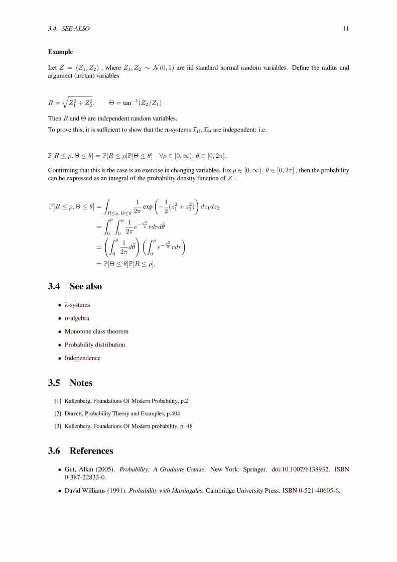
Let Z = (Z1, Z2) , where Z1, Z2 ∼ N (0, 1) are iid standard normal random variables. Define the radius andargument (arctan) variables

R =√

Z21 + Z2

2 , Θ = tan−1(Z2/Z1)

Then R and Θ are independent random variables.To prove this, it is sufficient to show that the π-systems IR, IΘ are independent: i.e.

P[R ≤ ρ,Θ ≤ θ] = P[R ≤ ρ]P[Θ ≤ θ] ∀ρ ∈ [0,∞), θ ∈ [0, 2π].

Confirming that this is the case is an exercise in changing variables. Fix ρ ∈ [0,∞), θ ∈ [0, 2π] , then the probabilitycan be expressed as an integral of the probability density function of Z .

P[R ≤ ρ,Θ ≤ θ] =

∫R≤ρ,Θ≤θ

1

2πexp

(−1

2(z21 + z22)

)dz1dz2

=

∫ θ

0

∫ ρ

0

1

2πe−

r2

2 rdrdθ

=

(∫ θ

0

1

2πdθ

)(∫ ρ

0

e−r2

2 rdr

)= P[Θ ≤ θ]P[R ≤ ρ].

3.4 See also• λ-systems

• σ-algebra

• Monotone class theorem

• Probability distribution

• Independence

3.5 Notes[1] Kallenberg, Foundations Of Modern Probability, p.2

[2] Durrett, Probability Theory and Examples, p.404

[3] Kallenberg, Foundations Of Modern probability, p. 48

3.6 References• Gut, Allan (2005). Probability: A Graduate Course. New York: Springer. doi:10.1007/b138932. ISBN0-387-22833-0.

• David Williams (1991). Probability with Martingales. Cambridge University Press. ISBN 0-521-40605-6.

12 CHAPTER 3. PI SYSTEM

3.7 Text and image sources, contributors, and licenses

3.7.1 Text• Dynkin system Source: https://en.wikipedia.org/wiki/Dynkin_system?oldid=598999646Contributors: CharlesMatthews, Giftlite, Lupin,

Skylarth, Bob.v.R, Rich Farmbrough, Paul August, Tsirel, Btyner, Sin-man, Rjwilmsi, Salix alba, RussBot, Natalie Packham, Thijs!bot,Vanish2, Nm420, Jmath666, SieBot, Melcombe, Addbot, Tcncv, Angry bee, DSisyphBot, 777sms, Cncmaster, ChrisGualtieri, Rank-onemap, DarenCline and Anonymous: 7

• Lebesguemeasure Source: https://en.wikipedia.org/wiki/Lebesgue_measure?oldid=682875664Contributors: AxelBoldt, Zundark,Miguel~enwiki,Patrick, Michael Hardy, TakuyaMurata, Loisel, Stevan White, Poor Yorick, Vargenau, Revolver, John Cross, Dcoetzee, Populus, Fi-bonacci, Tobias Bergemann, Pdenapo, Weialawaga~enwiki, Tosha, Giftlite, Lethe, MathKnight, Daniel Brockman, CSTAR, Vivacissama-mente, Rich Farmbrough, TedPavlic, Guanabot, Paul August, Bender235, Rbj, Obradovic Goran, Jumbuck, Uncle Bill, Oleg Alexandrov,Arneth, StradivariusTV,OdedSchramm, Graham87, JonathanZ, Chobot, Algebraist, YurikBot, Stormbay, Trovatore, CLW, Scriber~enwiki,Banus, SmackBot, MalafayaBot, Nbarth, Hongooi, Feraudyh, Naumz, Ejcaro, KazKylheku, CRGreathouse, CBM, David Cooke, E.G.,Bernard the Varanid, PKT, King Bee, Vantelimus, Salgueiro~enwiki, Jazzam, JAnDbot, Alokbakshi, Sullivan.t.j, Americanhero, Kope,Maurice Carbonaro, Owlgorithm, O.mangold, AlleborgoBot, Paolo.dL, Nnemo, Grubb257, CàlculIntegral, Addbot, Lightbot, Legobot,Luckas-bot, Yobot, Lucubrations, AnomieBOT, Erel Segal, Bdmy, FrescoBot, Rckrone, Citation bot 1, DrilBot, Wham Bam Rock II,Chiqago, Maschen, CountMacula, ChuispastonBot, Raiden10, Rezabot, Jorgecarleitao, CitationCleanerBot, JYBot, Stephan Kulla, Frosty,Ronoth, SoSivr, Mkroberson0208 and Anonymous: 60

• Pi system Source: https://en.wikipedia.org/wiki/Pi_system?oldid=681502917 Contributors: Charles Matthews, Salix alba, Wavelength,Spacepotato, Dmharvey, Stifle, Mattroberts, Ru elio, Vanish2, Sullivan.t.j, David Eppstein, TXiKiBoT, Kinrayfchen, Addbot, Aroch,Yobot, Hairer, DrilBot, Helpful Pixie Bot, BG19bot, Odaniel1, Savick01, Bwangaa, Egreif1, DarenCline, Cyrus Cousins and Anonymous:10

3.7.2 Images• File:Translation_of_a_set.svg Source: https://upload.wikimedia.org/wikipedia/commons/9/91/Translation_of_a_set.svg License: CC

BY 3.0 Contributors: Own work Original artist: Stephan Kulla (User:Stephan Kulla)

3.7.3 Content license• Creative Commons Attribution-Share Alike 3.0