Dynamic Programming Algorithm for Optimization of...

Dynamic Programming Algorithm forOptimization of β-Decision Rules

Talha Amin1, Igor Chikalov1, Mikhail Moshkov1, and Beata Zielosko1,2

1 Mathematical and Computer Sciences & Engineering DivisionKing Abdullah University of Science and Technology

Thuwal 23955-6900, Saudi Arabia{talha.amin,igor.chikalov,mikhail.moshkov,beata.zielosko}@kaust.edu.sa

2 Institute of Computer Science, University of Silesia39, Bedzinska St., 41-200 Sosnowiec, Poland

Abstract. We describe a dynamic programming algorithm that buildsa decision rule for each row of a decision table. Rules are constructed ac-cording to the minimum description length principle: they have minimumlength. Model complexity is regulated by adjusting rule accuracy.

Key words: decision rules, dynamic programming, minimization of de-cision rule length

1 Introduction

Decision rules are widely used for representation of knowledge extracted fromdata sets and for construction of classifiers that predict characteristics of newobjects on the basis of information on existing objects [13, 19].

Exact decision rules can be “overlearned”, i.e., may depend on the “noise”present in the input data. Therefore, recent years particular attention has beendevoted to approximate decision rules (which can be considered also as ap-proximate local reducts) and which are studied intensively by H.S. Nguyen, A.Skowron, D. Slezak, Z. Pawlak, J. Wroblewski and others [2, 9–12, 14, 15, 21–23].

In this paper, we consider one more approach to the definition of notion ofapproximate decision rule: we study so-called β-decision rules.

Models with shorter description are commonly believed to be more appro-priate among the models with similar accuracy (minimum description lengthprinciple [18]). Following this principle, we are interested in building the short-est β-decision rules.

In this paper, we study dynamic programming approach to optimizationof β-decision rules. Similar approach (but for optimization of another kind ofapproximate rules) was considered in [4, 25]

There are different approaches to construction of decision rules: brute-forceapproach which is applicable to tables with relatively small number of attributes,genetic algorithms [22, 24], simulated annealing [6], Boolean reasoning [11, 16,20], ant colony optimization [3, 7], algorithms based on decision tree construction

CONCURRENCY, SPECIFICATION AND PROGRAMMING M. Szczuka et al. (eds.): Proceedings of the international workshop CS&P 2011 September 28-30, Pułtusk, Poland, pp. 10-16

Dynamic Programming Algorithm for Optimization of β-Decision Rules 11

[8, 10, 17], different kinds of greedy algorithms [9, 11]. Each method can havedifferent modifications. For example, as in the case of decision trees, we can usegreedy algorithms based on Gini index, entropy, etc., for construction of decisionrules.

The most part of mentioned approaches (with the exception of brute-force oneand Boolean reasoning) cannot guarantee the construction of shortest rules. Weprove that our algorithm based on dynamic programming constructs β-decisionrules with minimum length.

The paper consists of five sections. In the second section, we discuss mainnotions. In the third section, we study dynamic programming algorithm forminimization of β-decision rule length. In the fourth section, we discuss resultsof experiments for datasets from [5]. The fifth section contains short conclusion.

2 Decision Tables and β-Decision Rules

Decision table is a rectangular table T with n columns filled with nonnegativeintegers. Columns of the table are assigned attributes f1, . . . , fn. Table rows arepairwise different, and each row r is labeled with a decision – a nonnegativeinteger. Table rows are interpreted as tuples of attribute values.

A decision attached to the maximum number of rows of T is called the mostcommon decision for T . If we have two or more such decisions, we choose thesmallest one. Denote by R(T ) the number of unordered pairs of rows from Twith different decisions.

A subtable of T is a table obtained from T by removing some rows with theirassigned decisions. Let j(1), . . . , j(k) ∈ {1, . . . , n} and b1, . . . , bk be nonnegativeintegers. Denote by T (fj(1), b1) . . . (fj(k), bk) the subtable of the table T , contain-ing the rows from T , which at the intersection with the columns fj(1), . . . , fj(k)have numbers b1, . . . , bk respectively. These subtables, including the table T , arecalled separable subtables of T .

Let r = (a1, . . . , an) be a row of the table T , i(1), . . . , i(m) ∈ {1, . . . , n}, andβ be a real number such that 0 ≤ β < 1. The expression

fi(1) = ai(1) ∧ . . . ∧ fi(m) = ai(m) → d (1)

is called a β-decision rule for r and T , if d is the most common decision forT ′ = T (fi(1), ai(1)) . . . (fi(m), ai(m)) and R(T ′) ≤ βR(T ). The number m is calledthe length of this decision rule.

Let Θ be a subtable of the table T , and r a row of Θ. We say that (1) is a(β, T )-decision rule for r and Θ, if R(Θ(fi(1), ai(1)) . . . (fi(m), ai(m))) ≤ βR(T ).A decision rule

→ d (2)

of length 0 is a (β, T )-decision rule for r and Θ if and only if R(Θ) ≤ βR(T ) andd is the most common decision for Θ. Note that the notion of (β, T )-decisionrule for r and T coincides with the notion of β-decision rule for r and T .


12 T. Amin, I. Chikalov, M. Moshkov, B. Zielosko

3 Dynamic Programming Algorithm for Optimization ofDecision Rules

3.1 Construction of Graph Gβ(T )

In this subsection, we describe an algorithm for constructing a directed acyclicgraph Gβ(T ) that is used in the rule optimization procedure.

Let Θ be a subtable of the table T . Denote by E(Θ) the set of attributes fi,for which at least two numbers are different in the column fi of the table Θ. Forfi ∈ E(Θ), denote by E(Θ, fi) the set of numbers contained in the column fi ofthe table Θ.

Consider an algorithm that constructs a directed acyclic graph Gβ(T ). Nodesof the graph are separable subtables of the table T . During each step, the algo-rithm processes one node and marks it with the symbol *. At the first step, thealgorithm constructs a graph containing a single node T .

Let the algorithm have already performed p steps. Let us describe the step(p + 1). If all nodes are marked with the symbol * as processed, the algorithmfinishes its work and presents the resulting graph as Gβ(T ). Otherwise, choose anode (table) Θ, which has not been processed yet. If R(Θ) ≤ βR(T ), then markΘ with the symbol * and go to the step (p + 2). Let R(Θ) > βR(T ). For eachfi ∈ E(Θ), draw a bundle of edges from the node Θ. Let E(Θ, fi) = {b1, . . . , bt}.Then draw t edges from Θ and label these edges with pairs (fi, b1), . . . , (fi, bt)respectively. These edges enter to nodes Θ(fi, b1), . . . , Θ(fi, bt). If some of nodesΘ(fi, b1), . . . , Θ(fi, bt) are absent in the graph then add these nodes to the graph.Mark the node Θ with the symbol * and proceed to the step (p+ 2).

Note that E(Θ) = ∅ implies Θ contains a single row (due to the fact thatthe rows of T are pairwise different) and, therefore, R(Θ) = 0 ≤ βR(T ).

3.2 Procedure of Optimization

Let us describe a procedure of optimization, that for each node Θ in the graphGβ(T ) assigns to each row r of Θ a (β, T )-decision rule for r and Θ.

We will move from the terminal nodes of the graph Gβ(T ) which do not haveany outgoing edges (R(Θ) ≤ βR(T ) for each node Θ of the kind), to the nodeT .

Let Θ be a terminal node. Assign to each row r of the table Θ the decisionrule (2) of length 0, where d is the most common decision for Θ.

Let Θ be a nonterminal node and all children of Θ already have decisionrules assigned to their rows. Let us assign a decision rule to each row r of thetable Θ. Let r = (a1, . . . , an). Consider all children of Θ containing the row rand choose among them a subtable Θ(fi, ai) that has a shortest decision ruleα→ d′ assigned to r. Assign the rule α ∧ fi = ai → d′ to the row r in the tableΘ.

Theorem 1. For any node Θ of the graph Gβ(T ) and any row r of the table Θ,the decision rule assigned to r by the optimization procedure is a (β, T )-decisionrule for r and Θ having minimum length.



Proof. We will prove this statement by induction on nodes (subtables) fromGβ(T ). It is clear that for each terminal node the considered statement is true.

Let Θ be a nonterminal node and for all children of Θ the considered state-ment hold. Let r = (a1, . . . , an) be a row of Θ. Then for some fi ∈ E(Θ) the rowr is labeled with a decision rule fi = ai∧αi → d where αi → d is the decision ruleattached to row r in the table Θ(fi, ai). According to the inductive hypothesis,the rule αi → d is a (β, T )-decision rule for r and Θ(fi, ai). Therefore the rulefi = ai ∧ αi → d is a (β, T )-decision rule for r and Θ.

Let us assume that there exists a shorter decision rule than fi = ai ∧αi → dwhich is a (β, T )-decision rule for r and Θ. Since Θ is a nonterminal node (andtherefore R(Θ) > βR(T )), the left-hand side of this shorter rule should containan equality of the kind fj = aj for some fj ∈ E(Θ). Thus this rule can berepresented in the form fj = aj ∧ α → d′. Since this rule is a (β, T )-decisionrule for r and Θ, the rule α → d′ is a (β, T )-decision rule for r and Θ(fj , aj).According to the inductive hypothesis, the row r in the table Θ(fj , aj) is labeledwith a rule γ → d′′ which length is at most the length of the rule α→ d′. Fromhere and from the description of the optimization procedure it follows that therow r in Θ is labeled with a rule which length is at most the length of the rulefj = aj ∧ γ → d′′ which is impossible. Therefore the rule attached to the row rin Θ has the minimum length among all rules which are (β, T )-decision rules forr and Θ . utCorollary 1. After completing the optimization procedure each row r of thetable T in the graph Gβ(T ) is assigned with a β-decision rule for r and T havingminimum length.

4 Preliminary Experimental Results

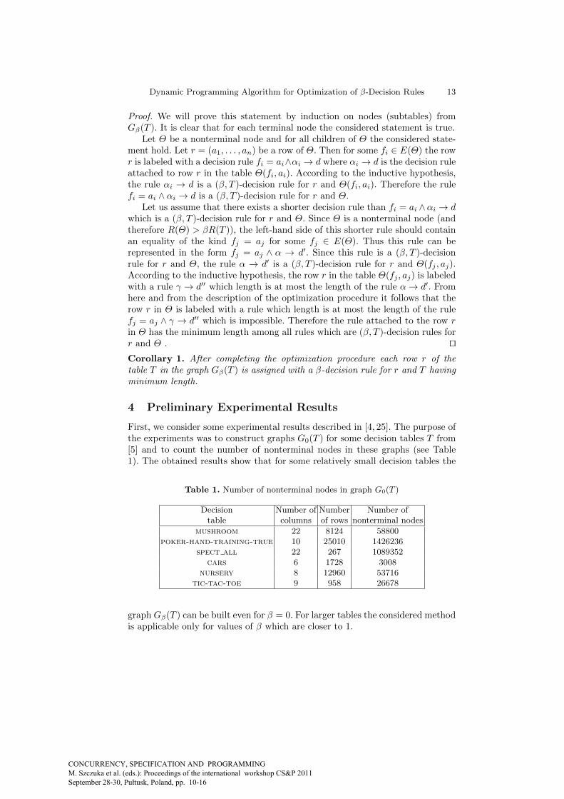
First, we consider some experimental results described in [4, 25]. The purpose ofthe experiments was to construct graphs G0(T ) for some decision tables T from[5] and to count the number of nonterminal nodes in these graphs (see Table1). The obtained results show that for some relatively small decision tables the

Table 1. Number of nonterminal nodes in graph G0(T )

Decision Number of Number Number oftable columns of rows nonterminal nodes

mushroom 22 8124 58800poker-hand-training-true 10 25010 1426236

spect all 22 267 1089352cars 6 1728 3008

nursery 8 12960 53716tic-tac-toe 9 958 26678

graph Gβ(T ) can be built even for β = 0. For larger tables the considered methodis applicable only for values of β which are closer to 1.



Table 2. Characteristics of DAG Gβ(T ) for the decision tables mushroom and cars

β mushroom cars# nodes # edges # nodes # edges

0 149979 2145617 7007 19886

0.001 59802 619898 1727 3420

0.01 24648 161983 473 688

0.1 4148 750874 118 129

0.2 1692 5302 22 21

We now consider results of experiments described in [1] with two datasetsfrom [5]: mushroom (8124 rows and 22 conditional attributes) and cars (1728rows and 6 conditional attributes). For β ∈ {0, 0.001, 0.01, 0.1, 0.2} we found thenumber of nodes in the directed acyclic graph Gβ(T ) and the number of edgesin Gβ(T ) (see Table 2). The obtained results show that the number of nodes andthe number of edges for Gβ(T ) decrease with the growth of β. It means that theparameter β can be used for managing algorithm complexity. They show alsothat the structure of graph Gβ(T ) is usually far from a tree: the number of edgesis essentially larger than the number of nodes.

Tables 3 and 4 contain results of experiments with three decision tables from[5]: balance scale, shuttle landing, and tic-tac-toe. For each row of

Table 3. Length of optimal rules

Dataset parameters β = 0 β = 0.01 β = 0.05# attr. # rows min avg max min avg max min avg max

balance scale 4 625 3 3.197 4 2 2.000 2 1 1.000 1

shuttle landing 6 15 1 1.400 4 1 1.400 4 1 1.200 4

tic-tac-toe 9 958 3 3.017 4 2 2.001 3 1 1.292 2

Table 4. Length of optimal rules

Dataset β = 0.1 β = 0.2 β = 0.3 β = 0.5min avg max min avg max min avg max min avg max

balance scale 1 1.000 1 1 1.000 1 1 1.000 1 1 1.000 1

shuttle landing 1 1.133 3 1 1.067 2 1 1.000 1 1 1.000 1

tic-tac-toe 1 1.081 2 1 1.000 1 1 1.000 1 1 1.000 1

these tables, for each value of β ∈ {0, 0.01, 0.05, 0.1, 0.2, 0.3, 0.5} we find a β-decision rule with minimum length (optimal rule). For each of the three decisiontables, Table 3 and Table 4 contain minimum length, maximum length andaverage length of optimal decision rules. We can see that the average length



of exact decision rules for balance scale and tic-tac-toe is about 3 and isdecreasing when β is growing. Beginning from β = 0.3 minimum, average andmaximum length of optimal rules for all datasets is equal to 1.

5 Conclusion

The paper is devoted to the consideration of one more type of approximate rules– β-decision rules. We designed an algorithm for minimization of β-decisionrule length and considered results of preliminary experiments. If we study exactrules (0-decision rules), then this algorithm is applicable to some relatively smalldecision tables. For large tables, we can work only with β-decision rules, whereβ should be not far from 1.

References

1. Alkhalid, A., Chikalov, I., Hussain, S., Moshkov, M.: Extensions of dynamic pro-gramming as a new tool for decision tree optimization. In: Ramanna, S., Howlett,R.J., Jain, L.C. (eds.) Emerging Paradigms in Machine Learning, Springer (toappear)

2. Bazan, G.J., Nguyen, S.H., Nguyen, T.T., Skowron, A., Stepaniuk, J.: Decisionrules synthesis for object classification. In: Or lowska, E. (ed.) Incomplete Informa-tion: Rough Set Analysis, pp. 23–57. Physica-Verlag, Heidelberg (1998)

3. Boryczka, U., Kozak, J.: New algorithms for generation decision trees – Ant-Minerand its modifications. Foundations of Computational Intelligence 6, 229–262 (2009)

4. Chikalov, I., Moshkov, M., Zielosko, B.: Online learning algorithm for ensemble ofdecision rules. In: Kuznetsov, S.O., Slezak, D., Hepting, D.H., Mirkin, B.G. (eds.)RSFDGrC 2011. LNCS (LNAI), vol. 6743, pp. 310–313. Springer, Heidelberg (2011)

5. Frank, A., Asuncion, A.: UCI Machine Learning Repository, http://archive.ics.uci.edu/ml

6. Jensen, R., Shen, Q.: Semantics-preserving dimensionality reduction: rough andfuzzy-rough-based approaches. IEEE Transactions on Knowledge and Data Engi-neering 16, 1457–1471 (2000)

7. Liu, B., Abbass, H.A., McKay, B.: Classification rule discovery with ant colonyoptimization. In: IEEE/WIC International Conference on Intelligent Agent Tech-nology, pp. 83–88. IEEE Computer Society, Washington, DC (2003)

8. Michalski, S.R., Pietrzykowski, J.: iAQ: A program that discovers rules. In: 22ndConference on Artificial Intelligence. Vancouver, Canada (2007)

9. Moshkov, M., Piliszczuk, M., Zielosko, B.: Partial Covers, Reducts and DecisionRules in Rough Sets: Theory and Applications. Studies in Computational Intelli-gence, vol. 145. Springer, Heidelberg (2008)

10. Moshkov, M., Zielosko, B.: Combinatorial Machine Learning: A Rough Set Ap-proach. Studies in Computational Intelligence, vol. 360. Springer, Heidelberg(2011)

11. Nguyen, H.S.: Approximate Boolean reasoning: foundations and applications indata mining. In: Peters, J.F., Skowron, A. (eds.) LNCS Transactions on RoughSets V. LNCS, vol. 4100, pp. 344–523. Springer, Heidelberg (2006)



12. Nguyen, H.S., Slezak, D.: Approximate reducts and association rules – correspon-dence and complexity results. In: Zhong, N., Skowron, A., Ohsuga, S. (eds.) RSFD-GrC 1999. LNCS (LNAI), vol. 1711, pp. 137–145. Springer, Heidelberg (1999)

13. Pawlak, Z.: Rough Sets – Theoretical Aspects of Reasoning about Data. KluwerAcademic Publishers, Dordrecht (1991)

14. Pawlak, Z.: Rough set elements. In: Polkowski, L., Skowron, A. (eds.) Rough Setsin Knowledge Discovery, pp. 10–30. Physica-Verlag, Heidelberg (1998)

15. Pawlak, Z., Skowron, A.: Rudiments of rough sets. Information Sciences 177, 3–27(2007)

16. Pawlak, Z., Skowron, A.: Rough sets and Boolean reasoning. Information Sciences177, 41–73 (2007)

17. Quinlan, J.R.: C4.5: Programs for Machine Learning. Morgan Kaufmann Publish-ers, San Mateo (1993)

18. Rissanen, J.: Modelling by shortest data description. Automatica 14, 465–471(1978)

19. Skowron, A.: Rough sets in KDD. In: 16th IFIP World Computer Congress, pp.1–14. Publishing House of Electronic Industry, Beijing (2000)

20. Skowron, A., Rauszer, C.: The discernibility matrices and functions in informationsystems. In: Slowinski, R. (ed.) Intelligent Decision Support. Handbook of Appli-cations and Advances of the Rough Set Theory, pp. 331–362. Kluwer AcademicPublishers, Dordrecht (1992)

21. Slezak, D.: Normalized decision functions and measures for inconsistent decisiontables analysis. Fundamenta Informaticae 44, 291–319 (2000)

22. Slezak, D., Wroblewski, J.: Order-based genetic algorithms for the search of approx-imate entropy reducts. In: Wang, G., Liu Q., Yao, Y., Skowron, A. (eds.) RSFDGrC2003. LNCS (LNAI), vol. 2639, pp. 308–311. Springer, Heidelberg (2003)

23. Wroblewski, J.: Ensembles of classifiers based on approximate reducts. FundamentaInformaticae 47, 351–360 (2001)

24. Wroblewski, J.: Finding minimal reducts using genetic algorithm. In: 2nd AnnualJoin Conference on Information Sciences. Wrightsville Beach, NC, pp. 186–189(1995)

25. Zielosko, B., Moshkov, M., Chikalov, I.: Optimization of decision rules based onmethods of dynamic programming. Vestnik of Lobachevsky State University ofNizhni Novgorod 6, 195–200 (2010) (in Russian)


Dynamic Programming Algorithm for Optimization of...

Documents

Transcript of Dynamic Programming Algorithm for Optimization of...