Dual Numbers: Simple Math, Easy C++ Coding, and Lots of Tricks

Gino van den Bergengino@dtecta.com

Introduction

Dual numbers extend the real numbers, similar to complex numbers.

Complex numbers adjoin a new element i, for which i2 = -1.

Dual numbers adjoin a new element ε, for which ε2 = 0.

Complex Numbers

Complex numbers have the form

z = a + b i

where a and b are real numbers. a = real(z) is the real part, and b = imag(z) is the imaginary part.

Complex Numbers (Cont’d) Complex operations pretty much

follow rules for real operators: Addition:

(a + b i) + (c + d i) = (a + c) + (b + d) i

Subtraction: (a + b i) – (c + d i) =

(a – c) + (b – d) i

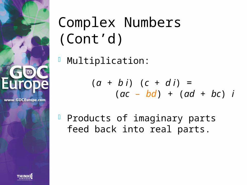
Complex Numbers (Cont’d) Multiplication:

(a + b i) (c + d i) = (ac – bd) + (ad + bc) i

Products of imaginary parts feed back into real parts.

Dual Numbers

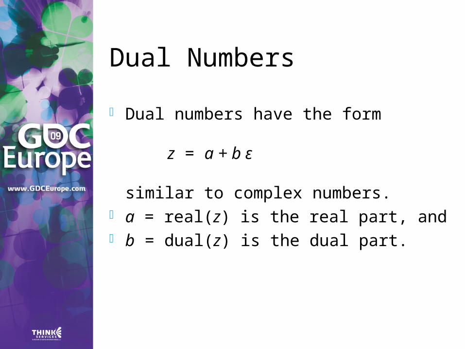
Dual numbers have the form

z = a + b ε

similar to complex numbers. a = real(z) is the real part, and b = dual(z) is the dual part.

Dual Numbers (Cont’d)

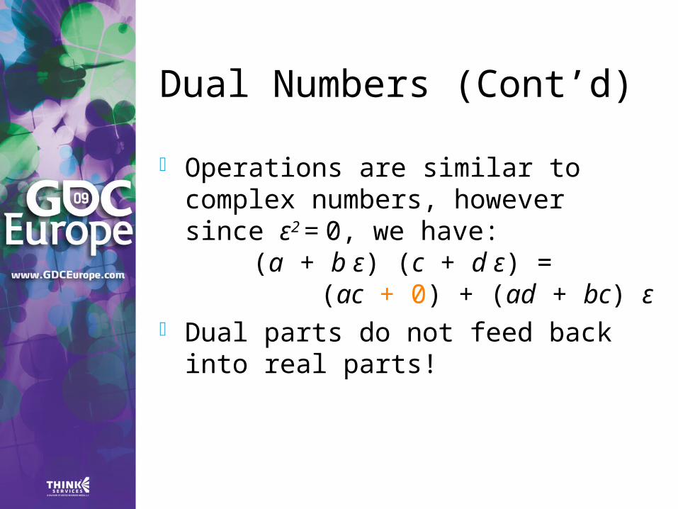
Operations are similar to complex numbers, however since ε2 = 0, we have:

(a + b ε) (c + d ε) = (ac + 0) + (ad + bc) ε

Dual parts do not feed back into real parts!

Dual Numbers (Cont’d)

The real part of a dual calculation is independent of the dual parts of the inputs.

The dual part of a multiplication is a “cross” product of real and dual parts.

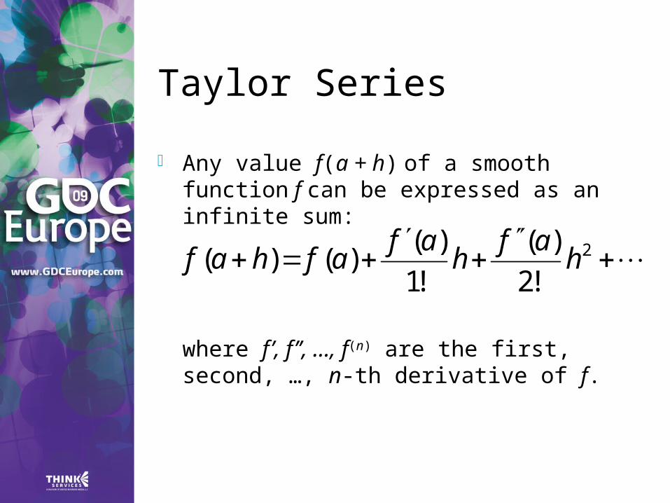
Taylor Series

Any value f(a + h) of a smooth function f can be expressed as an infinite sum:

where f’, f’’, …, f(n) are the first, second, …, n-th derivative of f.

2

!2

)(

!1

)()()( h

afh

afafhaf

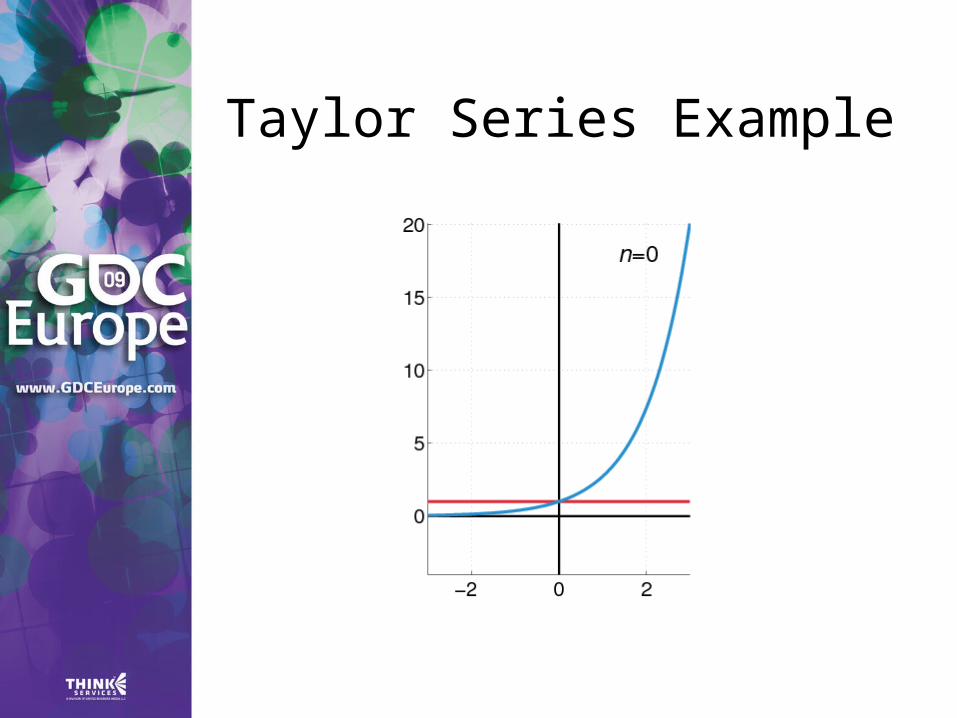
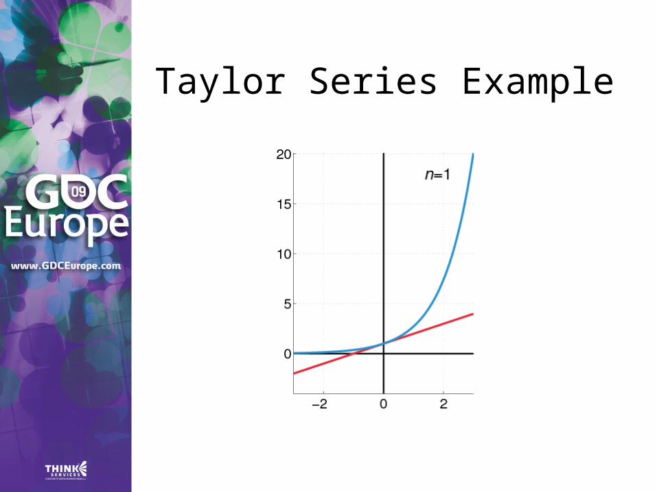
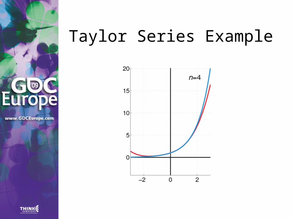
Taylor Series Example

Taylor Series Example

Taylor Series Example

Taylor Series Example

Taylor Series Example

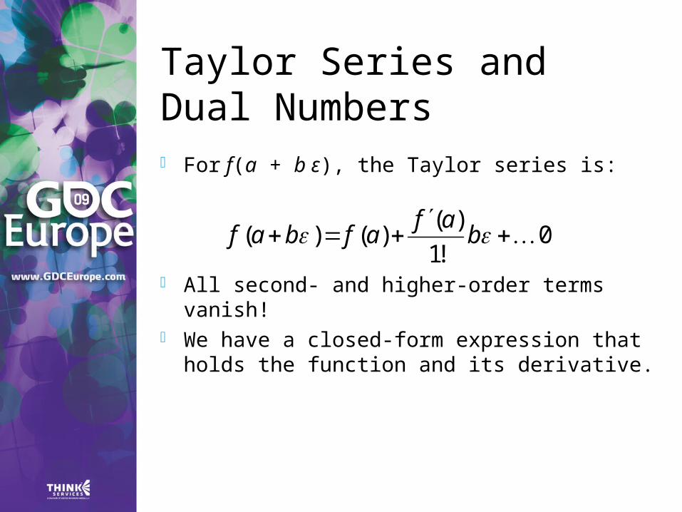
Taylor Series and Dual Numbers For f(a + b ε), the Taylor series is:

All second- and higher-order terms vanish!

We have a closed-form expression that holds the function and its derivative.

0!1

)()()(

b

afafbaf

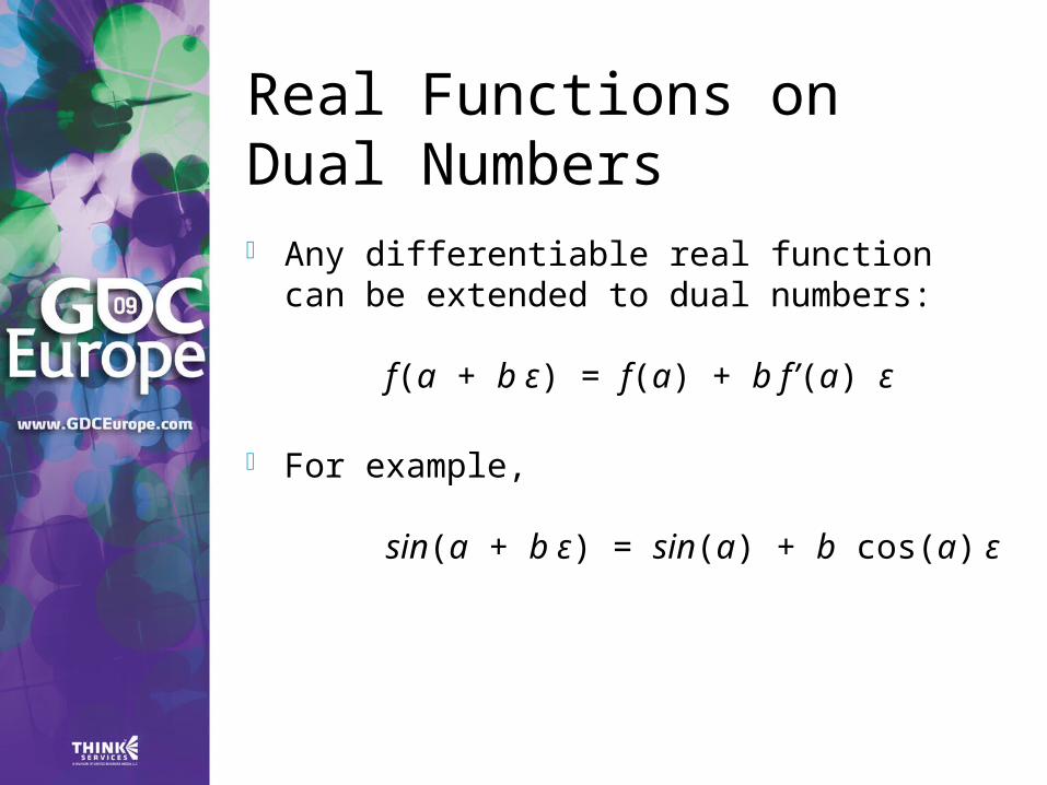
Real Functions on Dual Numbers Any differentiable real function can be

extended to dual numbers:

f(a + b ε) = f(a) + b f’(a) ε

For example,

sin(a + b ε) = sin(a) + b cos(a) ε

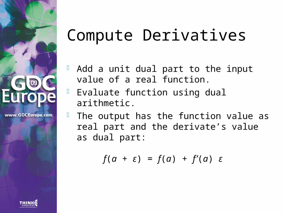
Compute Derivatives

Add a unit dual part to the input value of a real function.

Evaluate function using dual arithmetic. The output has the function value as

real part and the derivate’s value as dual part:

f(a + ε) = f(a) + f’(a) ε

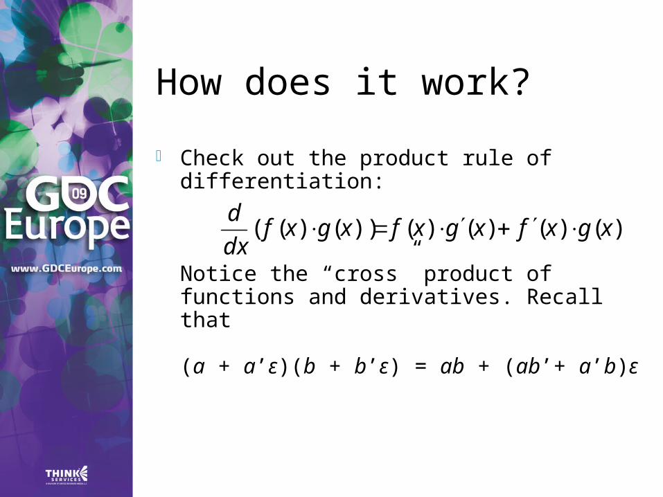
How does it work?

Check out the product rule of differentiation:

Notice the “cross” product of functions and derivatives. Recall that

(a + a’ε)(b + b’ε) = ab + (ab’+ a’b)ε

)()()()())()(( xgxfxgxfxgxfdx

d

Automatic Differentiation in C++ We need some easy way of

extending functions on floating-point types to dual numbers…

…and we need a type that holds dual numbers and offers operators for performing dual arithmetic.

Extension by Abstraction

C++ allows you to abstract from the numerical type through: Typedefs Function templates Constructors (conversion) Overloading Traits class templates

Abstract Scalar Type

Never use explicit floating-point types, such as float or double.

Instead use a type name, e.g. Scalar, either as template parameter or as typedef:

typedef float Scalar;

Constructors

Primitive types have constructors as well: Default: float() == 0.0f Conversion: float(2) == 2.0f

Use constructors for defining constants, e.g. use Scalar(2), rather than 2.0f or (Scalar)2 .

Overloading

Operators and functions on primitive types can be overloaded in hand-baked classes, e.g. std::complex.

Primitive types use operators: +,-,*,/ …and functions: sqrt, pow, sin, … NB: Use <cmath> rather than <math.h>.

That is, use sqrt NOT sqrtf on floats.

Traits Class Templates

Type-dependent constants, e.g. machine epsilon, are obtained through a traits class defined in <limits>.

Use std::numeric_limits<T>::epsilon() rather than FLT_EPSILON.

Either specialize this traits template for hand-baked classes or create your own traits class template.

Example Code (before)

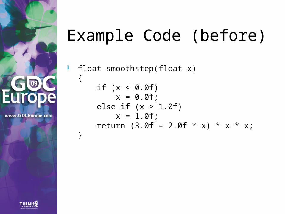
float smoothstep(float x){ if (x < 0.0f) x = 0.0f; else if (x > 1.0f) x = 1.0f; return (3.0f – 2.0f * x) * x * x;}

Example Code (after)

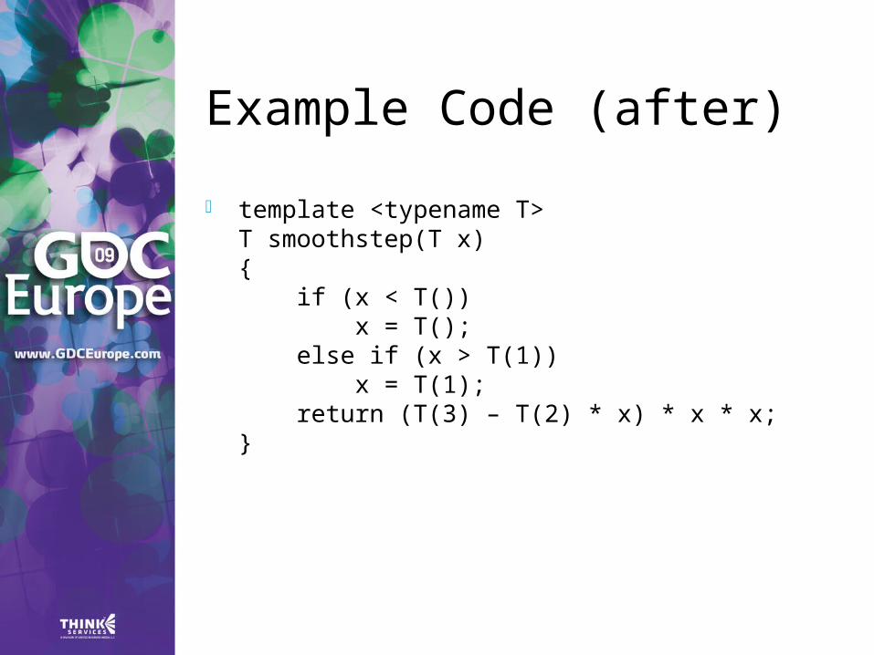
template <typename T>T smoothstep(T x){ if (x < T()) x = T(); else if (x > T(1)) x = T(1); return (T(3) – T(2) * x) * x * x;}

Dual Numbers in C++

C++ stdlib has a class template std::complex<T> for complex numbers.

We create a similar class template Dual<T> for dual numbers.

Dual<T> defines constructors, accessors, operators, and standard math functions.

Dual<T>

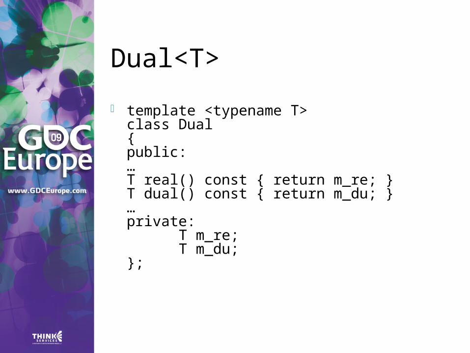
template <typename T>class Dual{public:…T real() const { return m_re; }T dual() const { return m_du; }…private:

T m_re; T m_du; };

Dual<T>: Constructor

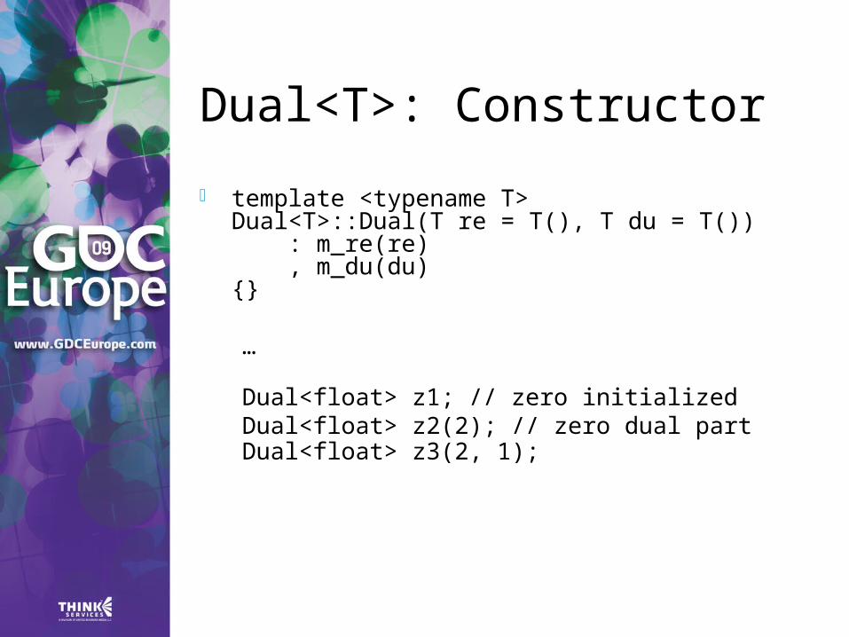
template <typename T>Dual<T>::Dual(T re = T(), T du = T()) : m_re(re) , m_du(du){}

…

Dual<float> z1; // zero initializedDual<float> z2(2); // zero dual part Dual<float> z3(2, 1);

Dual<T>: operators

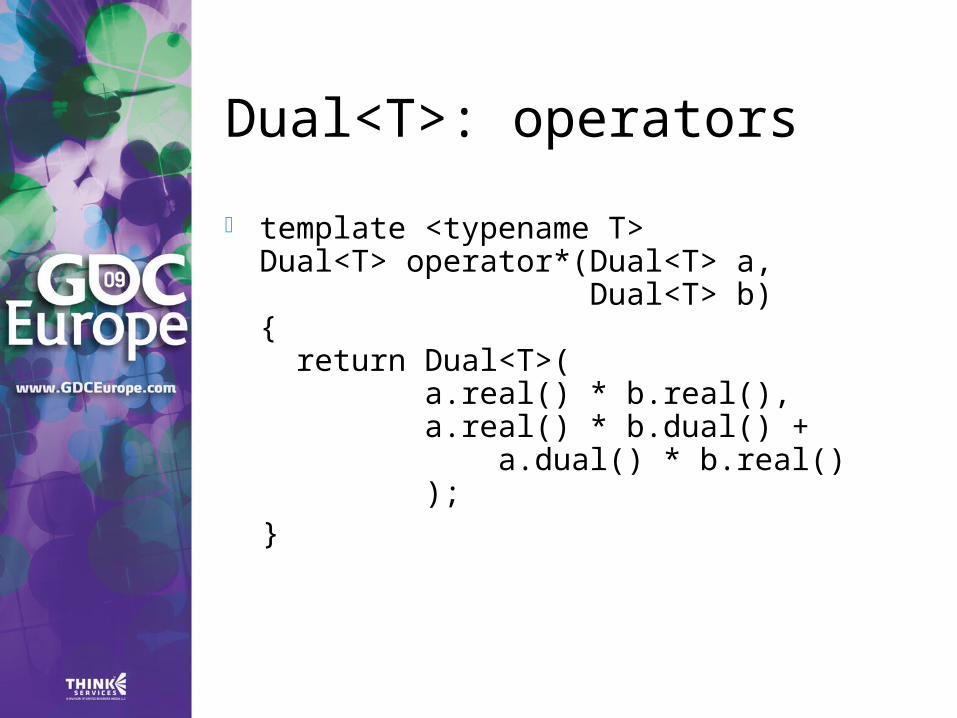
template <typename T>Dual<T> operator*(Dual<T> a, Dual<T> b){ return Dual<T>( a.real() * b.real(), a.real() * b.dual() + a.dual() * b.real() );

}

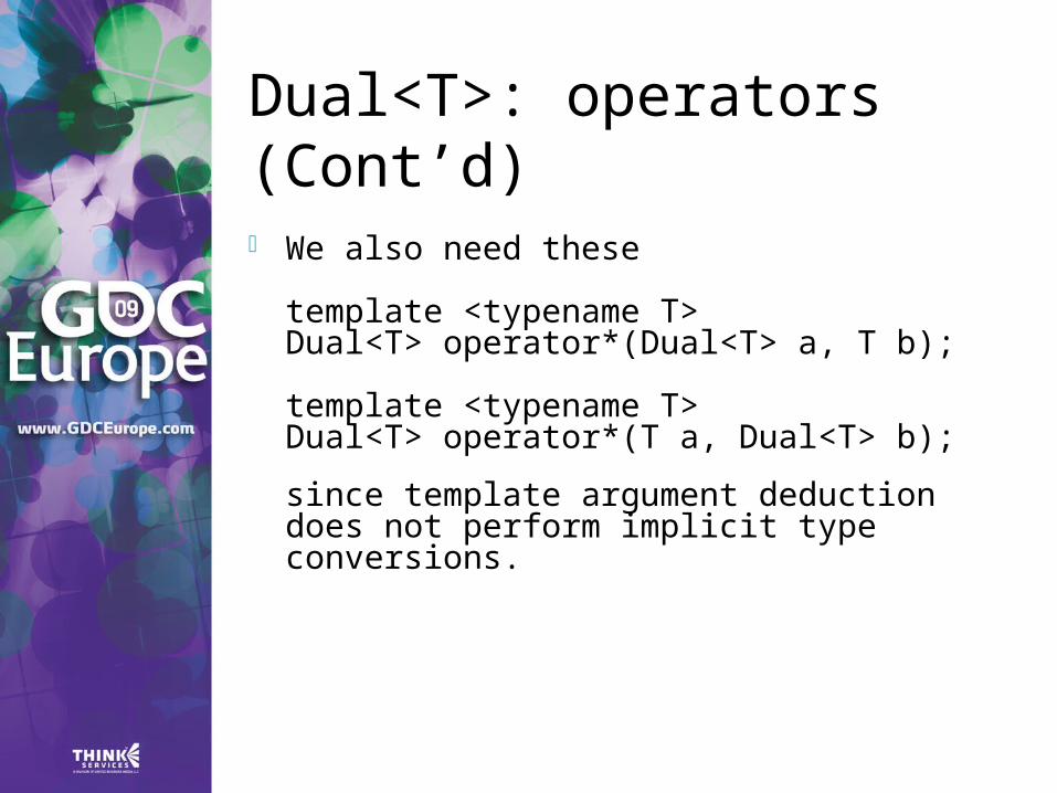
Dual<T>: operators (Cont’d) We also need these

template <typename T>Dual<T> operator*(Dual<T> a, T b);

template <typename T>Dual<T> operator*(T a, Dual<T> b);

since template argument deduction does not perform implicit type conversions.

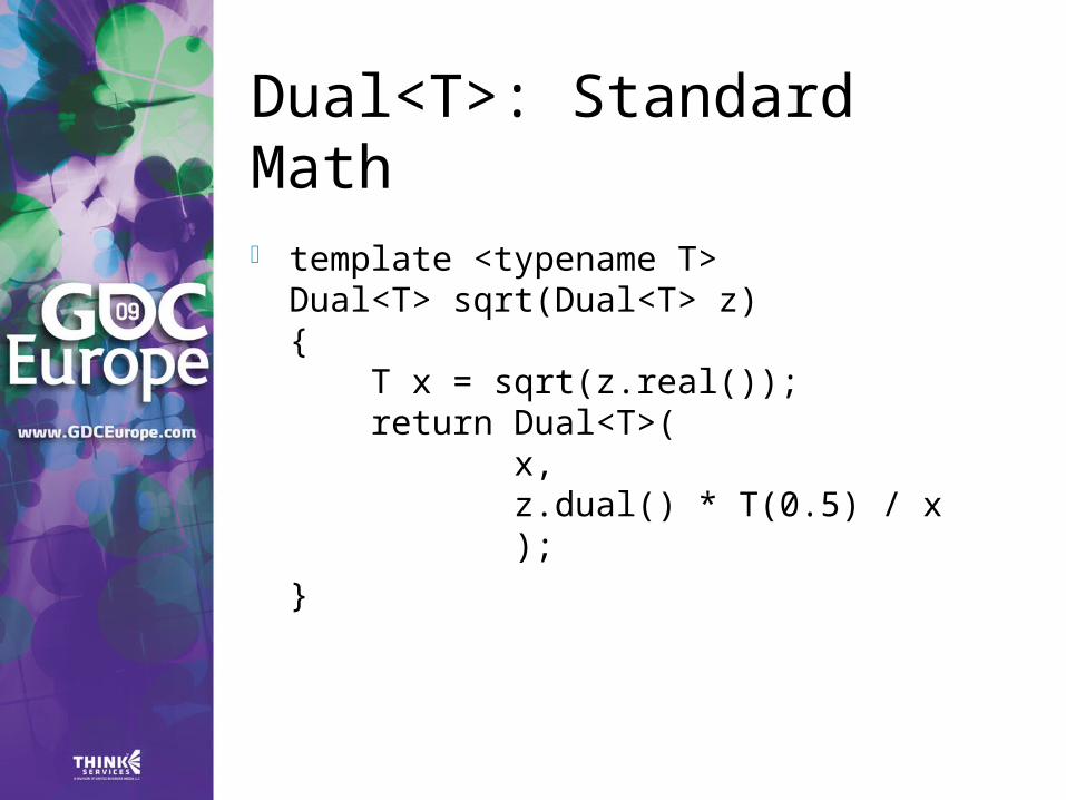
Dual<T>: Standard Math

template <typename T>Dual<T> sqrt(Dual<T> z){ T x = sqrt(z.real()); return Dual<T>( x, z.dual() * T(0.5) / x );

}

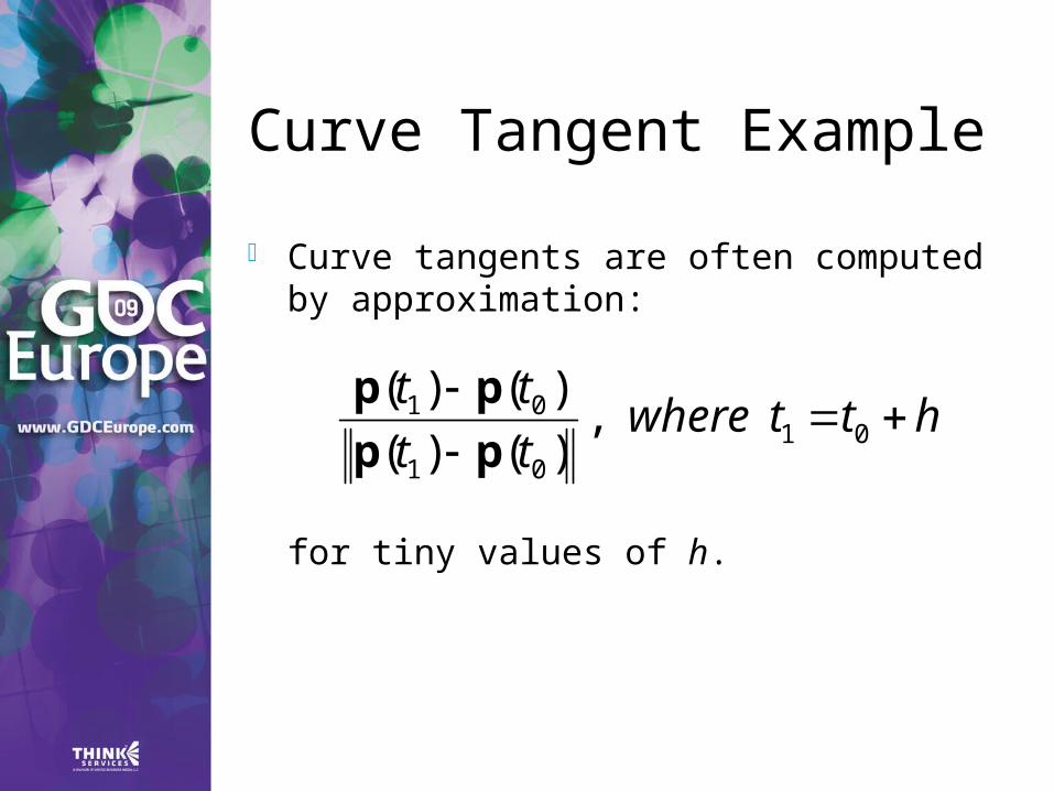
Curve Tangent Example

Curve tangents are often computed by approximation:

for tiny values of h.

httwherett

tt

0101

01 ,)()(

)()(

pp

pp

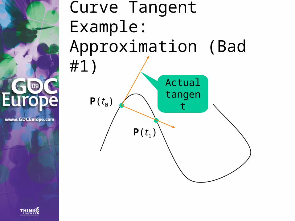
Curve Tangent Example:Approximation (Bad #1)

Actual tangentP(t0)

P(t1)

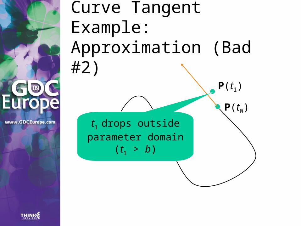
Curve Tangent Example:Approximation (Bad #2)

t1 drops outside parameter domain

(t1 > b)

P(t0)

P(t1)

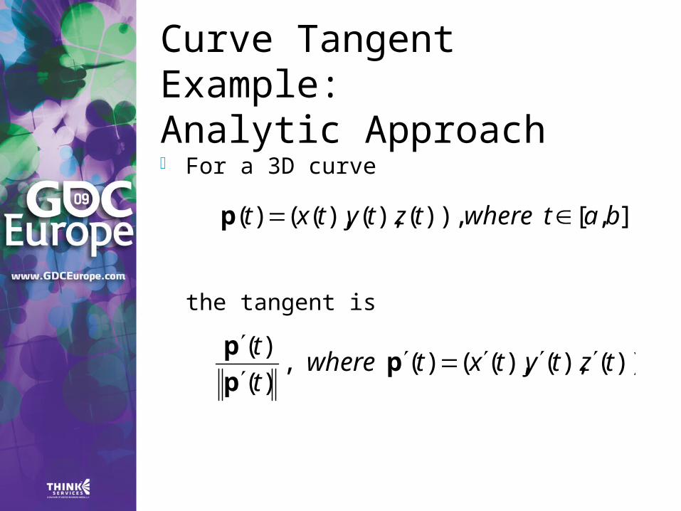
Curve Tangent Example:Analytic Approach For a 3D curve

the tangent is

],[)),(),(),(()( batwheretztytxt p

))(),(),(()(,)(

)(tztytxtwhere

t

t

pp

p

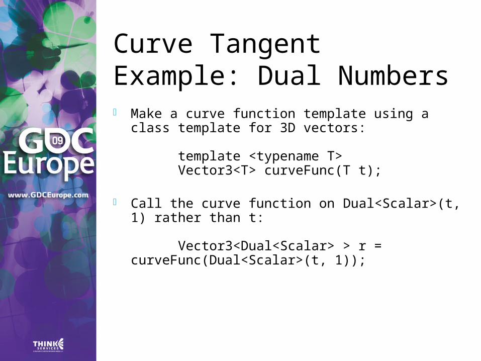
Curve Tangent Example: Dual Numbers Make a curve function template using a class

template for 3D vectors:

template <typename T>Vector3<T> curveFunc(T t);

Call the curve function on Dual<Scalar>(t, 1) rather than t:

Vector3<Dual<Scalar> > r = curveFunc(Dual<Scalar>(t,

1));

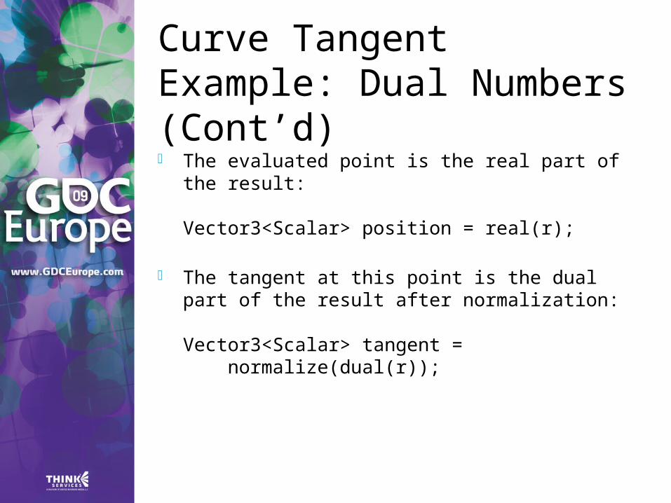
Curve Tangent Example: Dual Numbers (Cont’d) The evaluated point is the real part of the result:

Vector3<Scalar> position = real(r);

The tangent at this point is the dual part of the result after normalization:

Vector3<Scalar> tangent = normalize(dual(r));

Line Geometry

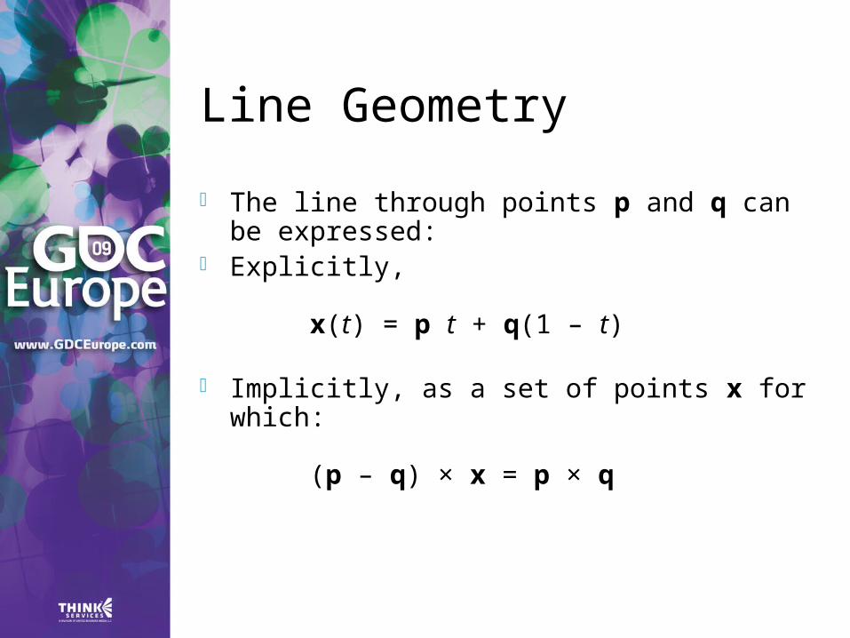
The line through points p and q can be expressed:

Explicitly,

x(t) = p t + q(1 – t)

Implicitly, as a set of points x for which:

(p – q) × x = p × q

Line Geometry

p

q0

p×q

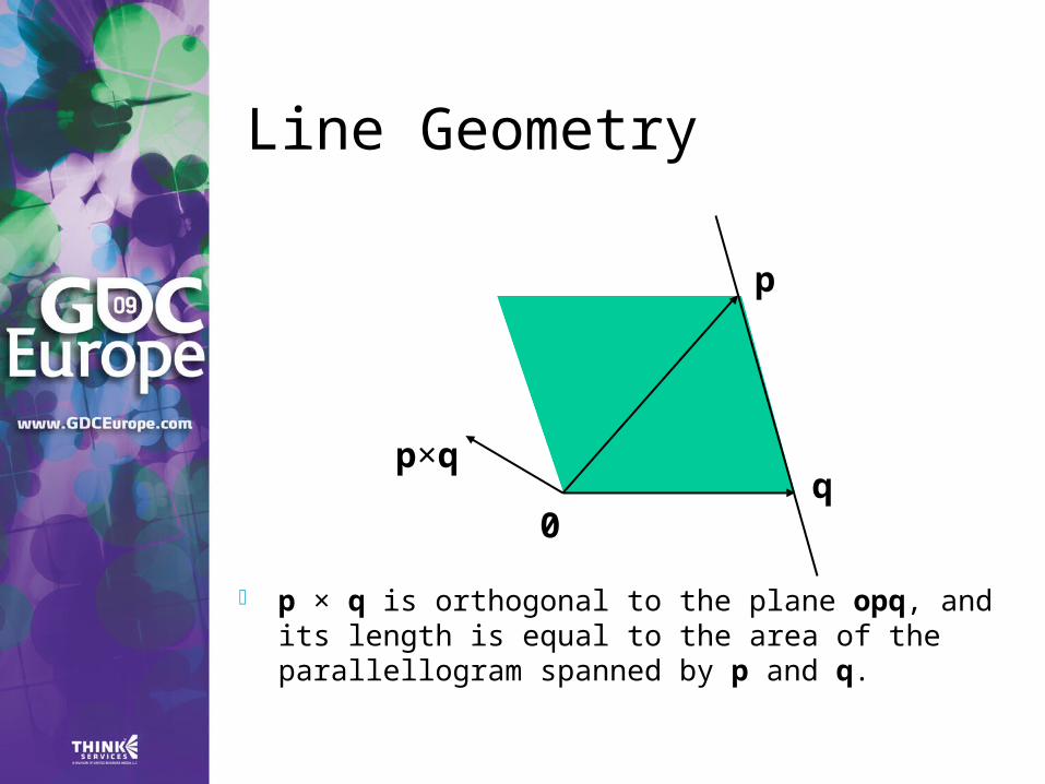
p × q is orthogonal to the plane opq, and its length is equal to the area of the parallellogram spanned by p and q.

Line Geometry

p

q0

p×qx

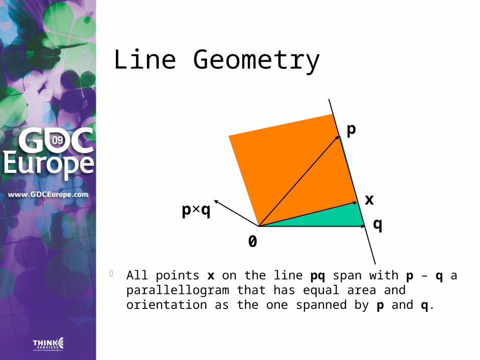
All points x on the line pq span with p – q a parallellogram that has equal area and orientation as the one spanned by p and q.

Plücker Coordinates

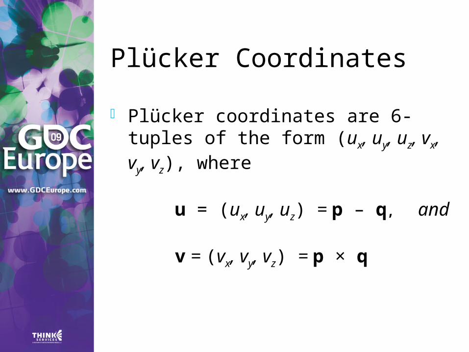
Plücker coordinates are 6-tuples of the form (ux, uy, uz, vx, vy, vz), where

u = (ux, uy, uz) = p – q, and

v = (vx, vy, vz) = p × q

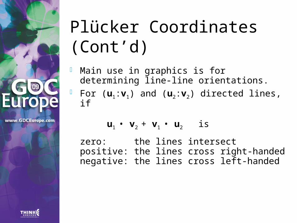
Plücker Coordinates (Cont’d) Main use in graphics is for determining

line-line orientations. For (u1:v1) and (u2:v2) directed lines, if

u1 • v2 + v1 • u2 is

zero: the lines intersectpositive: the lines cross right-handednegative: the lines cross left-handed

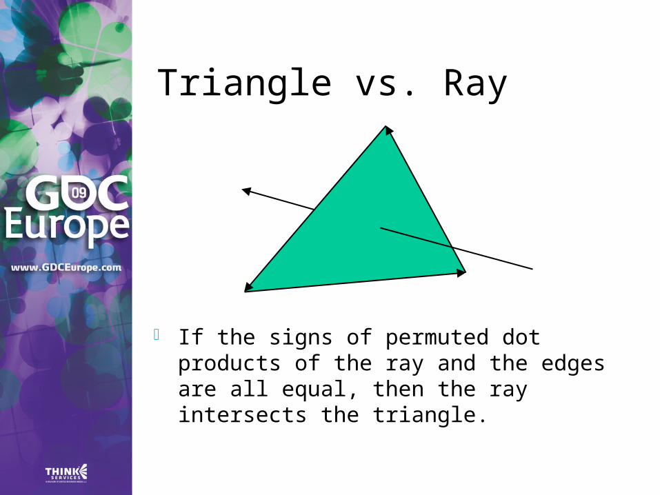
Triangle vs. Ray

If the signs of permuted dot products of the ray and the edges are all equal, then the ray intersects the triangle.

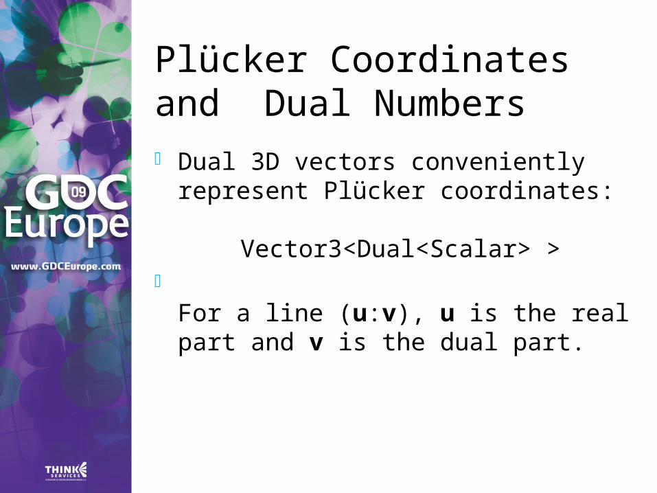
Plücker Coordinates and Dual Numbers Dual 3D vectors conveniently

represent Plücker coordinates:

Vector3<Dual<Scalar> >

For a line (u:v), u is the real part and v is the dual part.

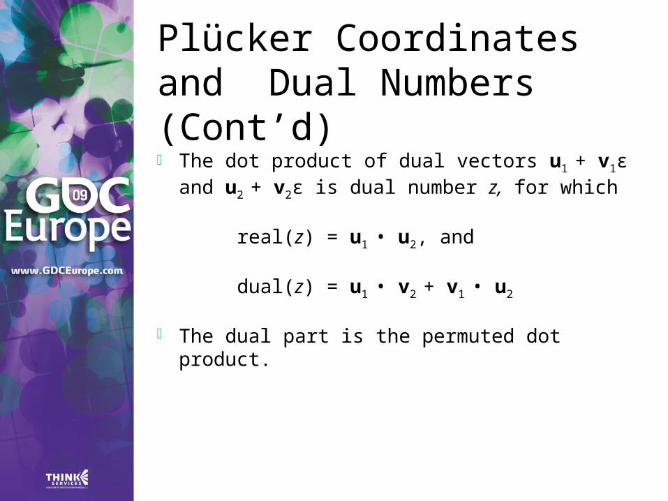
Plücker Coordinates and Dual Numbers (Cont’d) The dot product of dual vectors u1 + v1ε

and u2 + v2ε is dual number z, for which

real(z) = u1 • u2, and

dual(z) = u1 • v2 + v1 • u2

The dual part is the permuted dot product.

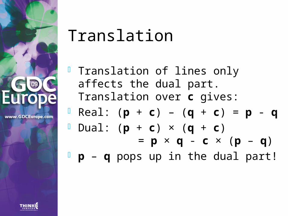
Translation

Translation of lines only affects the dual part. Translation over c gives:

Real: (p + c) – (q + c) = p - q Dual: (p + c) × (q + c)

= p × q - c × (p – q) p – q pops up in the dual part!

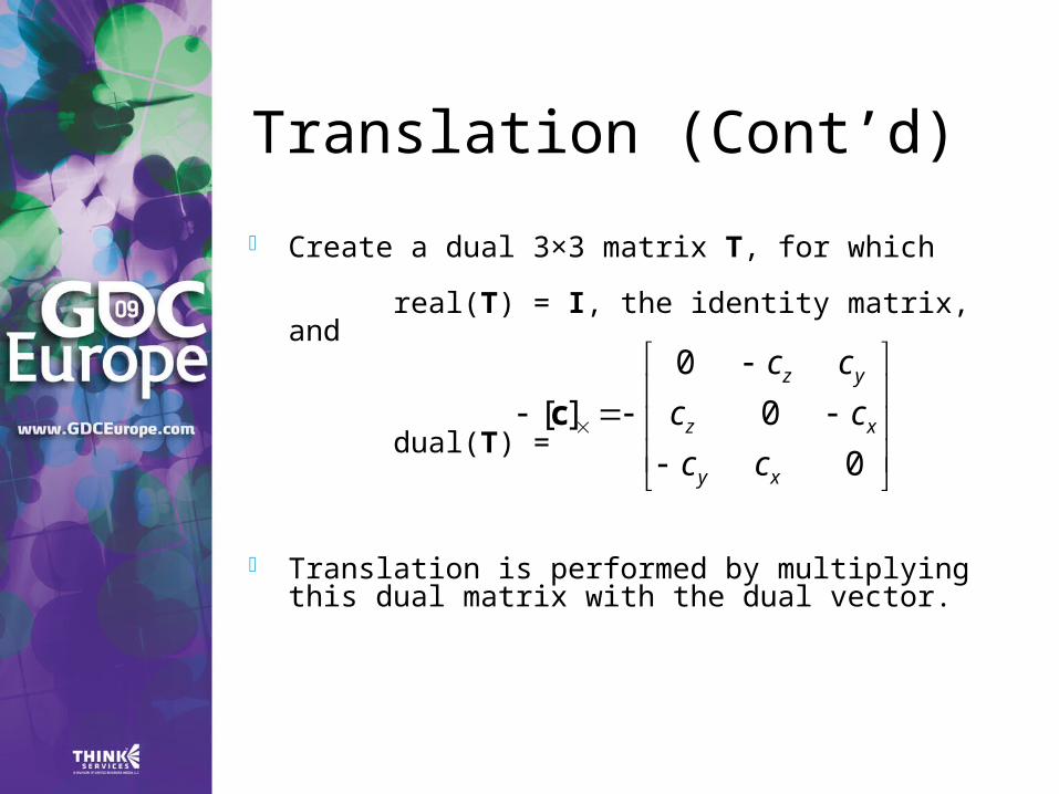
Translation (Cont’d)

Create a dual 3×3 matrix T, for which

real(T) = I, the identity matrix, and

dual(T) =

Translation is performed by multiplying this dual matrix with the dual vector.

0

0

0

][

xy

xz

yz

cc

cc

cc

c

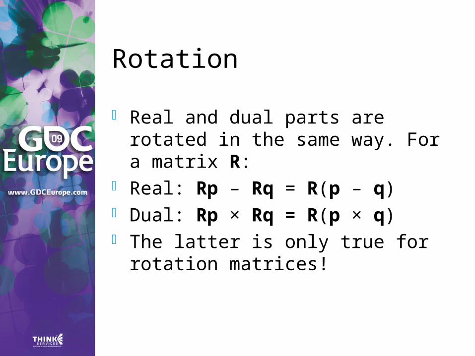
Rotation

Real and dual parts are rotated in the same way. For a matrix R:

Real: Rp – Rq = R(p – q) Dual: Rp × Rq = R(p × q) The latter is only true for rotation

matrices!

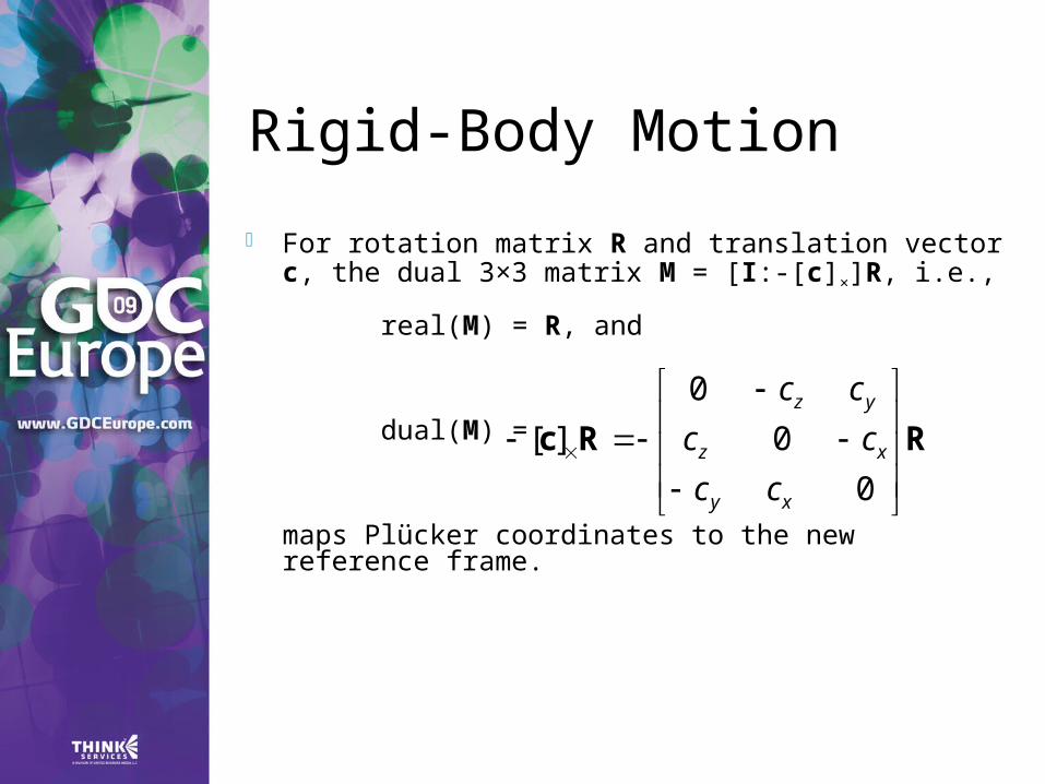
Rigid-Body Motion

For rotation matrix R and translation vector c, the dual 3×3 matrix M = [I:-[c]×]R, i.e.,

real(M) = R, and

dual(M) =

maps Plücker coordinates to the new reference frame.

RRc

0

0

0

][

xy

xz

yz

cc

cc

cc

Further Reading

Motor Algebra: Linear and angular velocity of a rigid body combined in a dual 3D vector.

Screw Theory: Any rigid motion can be expressed as a screw motion, which is represented by a dual quaternion.

Spatial Vector Algebra: Featherstone uses 6D vectors for representing velocities and forces in robot dynamics.

References

D. Vandevoorde and N. M. Josuttis. C++ Templates: The Complete Guide. Addison-Wesley, 2003.

K. Shoemake. Plücker Coordinate Tutorial. Ray Tracing News, Vol. 11, No. 1

R. Featherstone. Robot Dynamics Algorithms. Kluwer Academic Publishers, 1987.

L. Kavan et al. Skinning with dual quaternions. Proc. ACM SIGGRAPH Symposium on Interactive 3D Graphics and Games, 2007

Conclusions

Abstract from numerical types in your C++ code.

Differentiation is easy, fast, and accurate with dual numbers.

Dual numbers have other uses as well. Explore yourself!

Thank You!

Check out sample code soon to be released on:

http://www.dtecta.com