Domain Decomposition Methods for Flow in … Mathematics Volume 218, 1998 Domain Decomposition...

Contemporary MathematicsVolume 218, 1998

Domain Decomposition Methods for Flowin Heterogeneous Porous Media

Magne S. Espedal, Karl J. Hersvik, and Brit G. Ersland

1. Introduction

A reservoir may consist of several different types of sediments, which in generalhave different porosity, φ , absolute permeability, K , relative permeabilities, kri ,and capillary pressure Pc . In this paper we will study two phase, immiscible flow, inmodels consisting of one or two different types of sediment. Each of the sedimentsmay be heterogeneous. The phases are water (w) and oil (o), but the results mayeasily be extended to groundwater problems where the phases may be water andair or a non aqueous phase.

Such models represent a very complex and computational large problem anddomain decomposition methods are a very important part of a solution procedure.It gives a good tool for local mesh refinement in regions with large gradients suchas fluid fronts, interfaces between different sediments or at faults. If the modelsare heterogeneous, parameters in the models may be scale dependent, which meansthat mesh coarsening may be possible in regions with small gradients.

Let S = Sw denote the water saturation. Then the incompressible displacementof oil by water in the porous media can be described by the following set of partialdifferential equations, given in dimensionless form:

∇ · u = q1(x, t),(1)

u = −K(x)M(S,x)∇p,(2)

φ(x)∂S

∂t+∇ · (f(S)u)− ε∇ · (D(S,x)∇S) = q2(x, t) .(3)

Here, u is the total Darcy velocity, which is the sum of the Darcy velocities of theoil and water phases:

u = uo + uw

1991 Mathematics Subject Classification. Primary 76T05; Secondary 35M20, 65M55, 65M25.Key words and phrases. Reservoir models, Upscaling, Hierarchical basis, Domain

Decomposition, Operator splitting.Support from The Norwegian Research Council under the program PROPETRO and from

VISTA, a research cooperation between the Norwegian Academy of Science and Letters andStatoil, is gratefully acknowledged.

c©1998 American Mathematical Society

104

Contemporary Mathematics

Volume 218, 1998

B 0-8218-0988-1-03005-3

DD METHODS FOR FLOW IN HETEROGENEOUS POROUS MEDIA 105

Γ

K K

Ω Ω21

1 2

ProductionInjection

0

1

2

3

4

5

6

7

8

9

10

0 0.2 0.4 0.6 0.8 1

Diffusion.

K=1K=5

K=10

(a) (b)

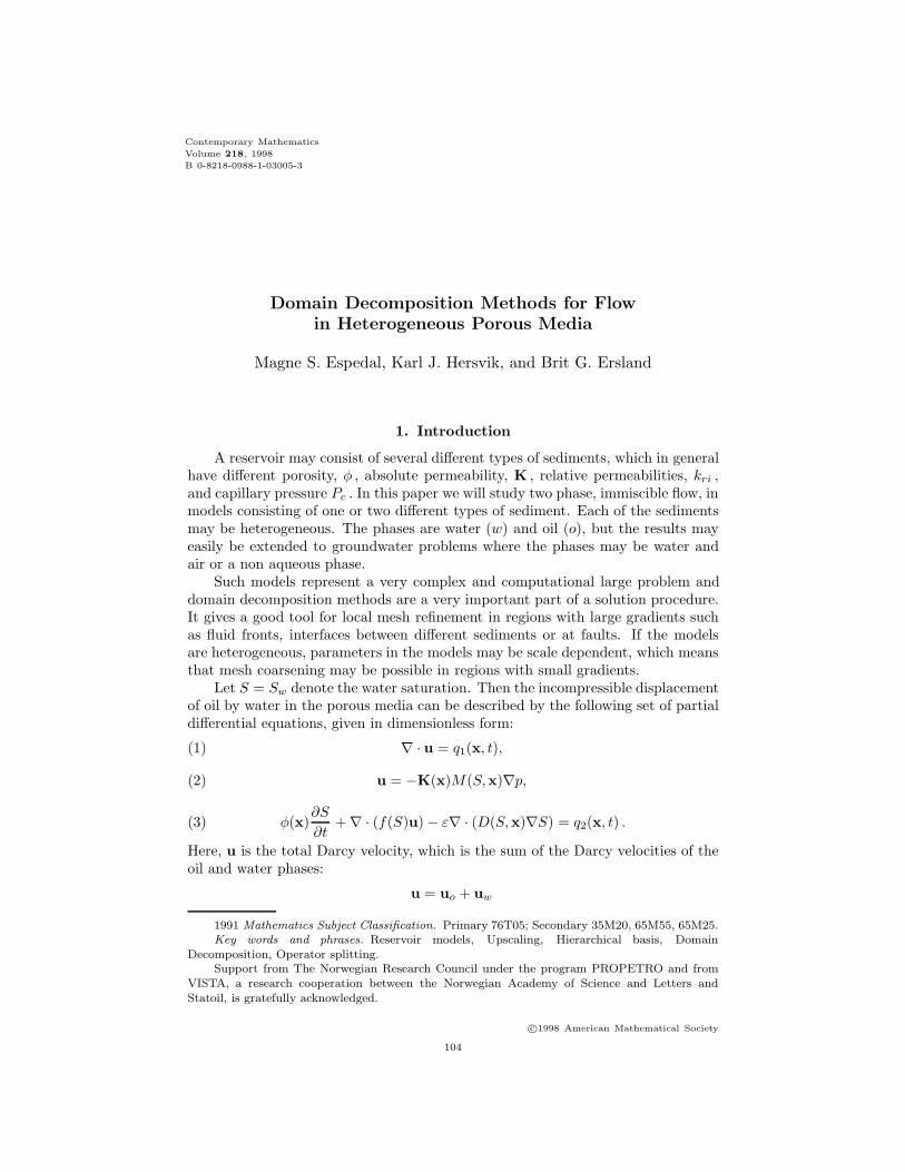
Figure 1. (a) Computational domain showing two differentregions with different physical properties connected through aninterior boundary Γ. (b) Capillary diffusion, as functions ofsaturation shown for permeabilities 1, 5 and 10.

Furthermore, p is the total fluid pressure given by p = 12 (pw + po), qi(x, t), i =

1, 2 denotes contribution from the injection and production wells in addition tocapillary pressure terms, which are treated explicitly in (1). K(x) is the absolutepermeability, M(S,x) denotes the nonzero total mobility of the phases and φ(x) isthe porosity. A reasonable choice for the porosity is φ = 0.2. The parameter ε is asmall (10−1 − 10−4) dimensionless scaling factor for the diffusion.

Equation (3) is the fractional flow formulation of the mass balance equationfor water. The fractional flow function f(S) is typically a S shaped function ofsaturation., The capillary diffusion function D(S,x) is a bell shaped function ofsaturation, S, and has an almost linearly dependence of the permeability K(x).Further, D(0,x) = D(1,x) = 0. In Figure 1, a capillary diffusion function is shownfor different permeabilities.

For a complete survey and justification of the model we refer to [5]. Wehave neglected gravity forces, but the methods described can also be applied formodels where gravity effects are included [17]. The following analytical form forthe capillary pressure is chosen[35]:

PC(S,x) = 0.9φ−0.9K−0.1 1− S√S,(4)

We note that the capillary pressure depend on the permeability of the rock.The phase pressures and the capillary pressure are continuous over a boundary

Γ, separating two sediments. Furthermore, the flux must be continuous [12, 14, 4,23] which gives the following internal boundary conditions:

PΓ−C (SΓ−) = PΓ+

C (SΓ+)(5)

(uΓ− − uΓ+) · nΓ = 0(6)

106 MAGNE S. ESPEDAL ET AL.

+ ++ -+

+ +- -

- +- +

- ++

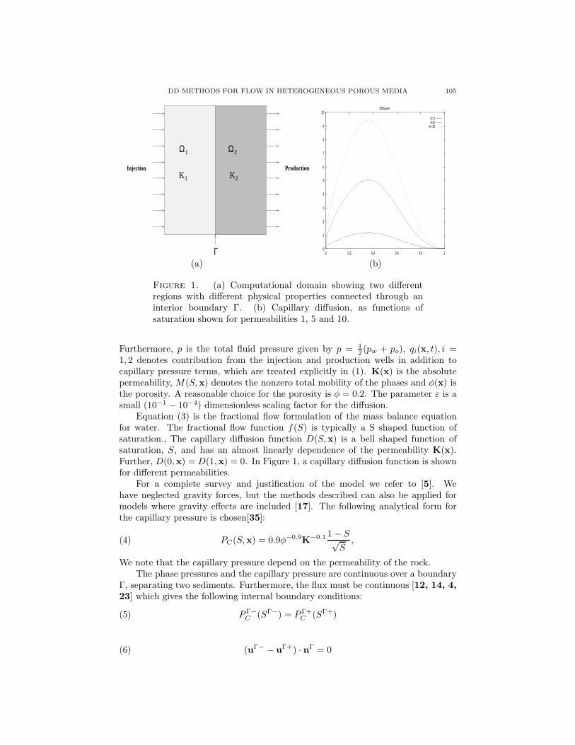
Figure 2. From left to right Γ0, Γα, Γβ, Γγ . The + and − signrepresent the functional value +1 and -1. Γ0 is the scaling function.

(f(SΓ−)u− εDΓ−(SΓ−,x)∇SΓ−) · nΓ = (f(SΓ+)u− εDΓ+(SΓ+,x)∇SΓ+) · nΓ.

(7)

Here (·)Γ− and (·)Γ+ denote the left and right hand side value at the interiorboundary Γ , and nΓ is normal to the boundary.

Since the capillary pressure depends on both the saturation and thepermeability, the continuity of the capillary pressure leads to discontinuessaturation over the interior boundary. Also, the flux conservation (7) create largegradients in the saturation over an interior boundary separating two differentsediments. This adds extra complexity to our problem especially when a saturationfront passes an interface.

2. Representation of the Permeability

The permeability K may have several orders of variation and the geometricaldistribution can be very different in the sediments. Further, fractures and faultsadd to the complexity. Therefore, we need a good method for the representation ofK. Hierarchical basis may be such a tool [27, 18].

The simplicity of the Haar system makes it an attractive choice for such arepresentation. Further it gives a permeability representation which is consistentwith a domain decomposition solution procedure. We will restrict ourselves to twospace dimensions and consider the unit square as our computational domain Ω.The Haar basis of scale 0 and 1, for two space dimension, is given by the set offunctions in Figure 2.

On each mesh of 2 × 2 cells, any cell wise constant function can be given arepresentation as linear combinations of Γ0, Γα, Γβ and Γγ , where the coefficientof Γ0 has a nonzero coefficient only for mesh of scale 0, which is the wholecomputational domain Ω. A 2-scale Haar multi resolution analysis, built on thescaling function Γ0 [6, 9], will be used to represent the permeability.

Let the absolute permeability K be a cell-wise constant function on Ω with2N+1 cells in each direction.

Then K can then be expanded in terms of the Haar basis:

K = K0Γ0 +N∑i=1

2N∑j=0

2N∑k=0

∑l=α,β,γ

KijklΓijkl(8)

where the index i gives the scale and j and k give the translations of the twodimensional wavelet Γijkl.


We should note that this representation is easily extended to three spacedimensions. If the permeability is given by a tensor, the wavelet representationshould be used for each of the components. Also, other types of wavelet may beused. Especially if an overlapping domain decomposition method is used, a lesslocalised wavelet representation should be useful.

3. Solution procedure

The governing equations (1), (2) and (3) are coupled. A sequential, timemarching strategy is used to decouple the equations. This strategy reflects thedifferent natures of the elliptic pressure equation given by (1) and (2), and theconvection dominated parabolic saturation equation (3). The general solutionstrategy is published earlier [15, 10, 25, 8, 21], so we only give the main steps inthe procedure.

3.1. Sequential Solution Procedure:

• Step 1:For t ∈ [tn, tn+1], solve the pressure and velocity equations (1, 2). Thevelocity is a smoother function in space and time than the saturation.Therefore we linearize the pressure and velocity equations by using thesaturation from the previous time step, S = S(tn) . The pressure equationis solved in a weak form, using a standard Galerkin method with bilinearelements [2, 31].

Then the velocity is derived from the Darcy equation (2), using localflux conservation over the elements [31]. This gives the same accuracy forthe velocity field as for the pressure. The mixed finite element method wouldbe an alternative solution procedure. In many cases, it is not necessary tosolve the pressure for each timestep.• Step 2:

A good handling of the convective part of the saturation equations, is essen-tial for a fast and accurate solution for S. We will use an operator splittingtechnique where an approximate saturation S is calculated from a hyper-bolic equation:For t ∈ [tn, tn+1], with u given from Step 1, solve:

dS

dτ≡ φ∂S

∂t+∇ · (f(S)u) = 0(9)

where f is a modified fractional flow function [15, 8, 21].• Step 3:

The solution S provide a good approximation of the time derivative and thenonlinear coefficients in (3).For t ∈ [tn, tn+1], and S0 = S, solve:

∂Si∂τ

+∇ · (b(Si−1)Siu−D(Si−1) · ∇Si) = q2(x, t)(10)

for i = 1, 2, 3.... until convergence, where b(S)S = f(S) − f(S). Equation(10) is solved in a weak form [15, 8], using optimal test functions [3].


• Step 4:Depending on the strength of the coupling between the velocity and thesaturation equation, the procedure may be iterated.

3.2. Domain decomposition. The pressure (1), (2) and saturation equation(10) represent large elliptic problems. The equations are solved by using apreconditioned iterative procedure, based on domain decomposition [32]. Theprocedure allows for adaptive local grid refinement, which gives a better resolutionat wells and in regions with large permeability variations such as interfaces betweentwo types of sediments. The procedure also allows for adaptive local refinementat moving saturation fronts. Assuming a coarse mesh ΩC on the computationaldomain Ω, we get the following algorithm [29, 8, 34, 33]:

1. Solve the splitted hyperbolic saturation equation (9) on the coarse grid ΩC ,by integrating backwards along the characteristics.

2. Identify coarse element that contain large gradients in saturation andactivate refined overlapping/non overlapping sub grids Ωk to each of these.

3. Solve equation (9) on the refined sub grids Ωk, by integrating backwardsalong the characteristics.

4. Using domain decomposition methods, solve the complete saturationequation with the refined coarse elements. The characteristic solution Sis used as the first iteration of the boundary conditions for the sub domainsΩk .

As is well known, algorithms based on domain decompositions have good parallelproperties [32].

We will present result for 2D models, but the procedure has been implementedand tested for 3D models [16].

4. Coarse Mesh Models

With the solution procedure described in Section 3, pressure, velocity andsaturation will be given on a coarse mesh in some regions a and on a refined meshin the remaining part of Ω. This means that the model equations have to begiven for different scales. Several upscaling techniques are given in the literature[22, 1, 11, 26, 18, 7, 30, 24]. In this paper, we will limit the analysis to theupscaling of the pressure equation. The upscaling of the saturation equation is lessstudied in the literature [1, 24].

The goal of all upscaling techniques is to move information from a fine grid to acoarser grid without loosing significant information along the way. A quantitativecriteria is the conservation of dissipation:

e = K∇p · ∇p(11)

A related and intuitively more correct criteria, is the conservation of the mean fluidvelocity 〈v〉, given by:

〈v〉 = −Keff∇〈p〉∇ · 〈v〉 = 0(12)

where Keff is an effective permeability.In our approach it is natural to use conservation of the mean velocity as the

upscaling criteria, although the method also conserves dissipation fairly well [18].


4.1. Wavelet upscaling. A Multi Resolution Analysis (MRA), [9], definedon L2(R)×L2(R) consists of a nested sequence of closed subspaces of L2,×L2 suchthat:

· · · ⊂ V1 ⊂ V0 ⊂ V−1 ⊂ · · ·(13) ⋃j∈Z Vj = L2(R)× L2(R)(14) ⋂

j∈Z Vj = 0(15)

Vj+1 = Vj ∪Wj(16)f(x) ∈ Vj ⇐⇒ f(2x) ∈ Vj+1(17)

Here, Wj is the orthogonal complement of Vj in Vj+1. The permeability givenby (8) satisfies such a hierarchical representation. Let j = 0 and j = J berespectively the coarsest and finest scale to appear in K. Upscaling in this contextis to move information form scale j = J to a coarser scale j = M , M ≤ J .

In signal analysis, ”highcut” filters are commonly used to clean a signal fromits high frequency part which is considered to be negligible noise. We will apply tosame reasoning on K. Such an upscaling will keep all large scale information, whilevariation on scales below our course grid will be neglected in regions where the flowhas a slow variation. Moderate fine scale changes in the permeability, give rise toheterogeneous fingers [24] and have little influence on the global transport. Butthis upscaling technique is only valid in the case that the coefficients on the scalesJ, J − 1, . . . ,M are small compared to the coefficients on a lower scale. This wouldnot be the case for narrow high permeability zones. However, in regions with highpermeability channels, the solutions will contain large gradients, which mean thatwe should use a refined grid to resolve the dynamics. A coarse grid solution basedon upscaling, will loose too much information in such regions.

4.2. Highcut upscaling. We will give an example of the highcut upscalingtechniques on an anisotropic permeability field. Such a field is chosen because itis difficult to handle using simple mean value techniques. The coefficients whichdetermine the permeability field at each scale are read from a file, but if we want towork with measured permeability fields, a subroutine can determine the coefficientson each scale recursively using standard two scale relations from the wavelet theory,[9].

The permeability field is generated by introducing large coefficients on arelatively low level. The goal is to model a case where we may have several regimes ofpermeability which on their own may be isotropic, but when put together constitutea very complex reservoir.

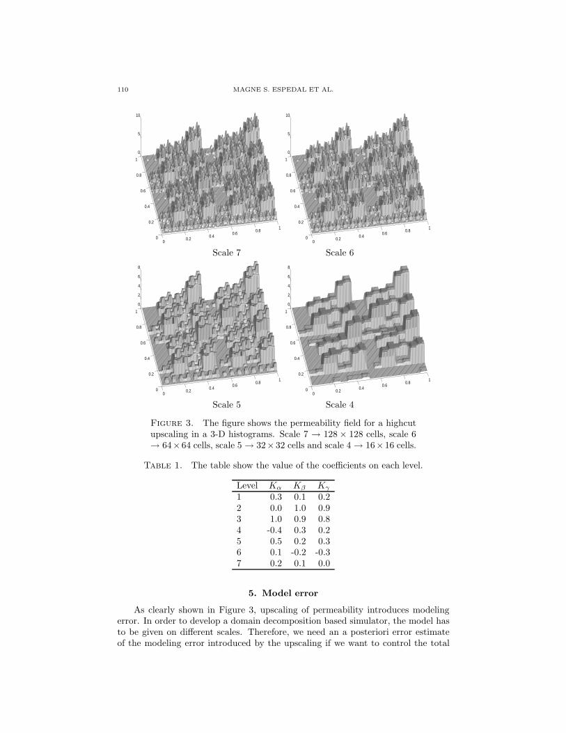
Figure 3 shows the permeability field for a highcut upscaling as 3-D histograms.We can clearly see the complexity and anisotropy of the permeability field.Upscaling to scale 3 gives a massive loss of information, because the scale 4coefficient are fairly large.

Table 1 displays the coefficients used. The aspect ratio between the highestand lowest permeability is about 10 in this case [18]. The highest scale is 7 whichgives 27 × 27 cells, and the permeability value on scale 0 is 1.0. Kα, Kβ and Kγ

are the coefficients of Γα, Γβ and Γγ respectively (2).


00.2

0.40.6

0.81

0

0.2

0.4

0.6

0.8

1

0

5

10

00.2

0.40.6

0.81

0

0.2

0.4

0.6

0.8

1

0

5

10

Scale 7 Scale 6

00.2

0.40.6

0.81

0

0.2

0.4

0.6

0.8

1

0

2

4

6

8

00.2

0.40.6

0.81

0

0.2

0.4

0.6

0.8

1

0

2

4

6

8

Scale 5 Scale 4

Figure 3. The figure shows the permeability field for a highcutupscaling in a 3-D histograms. Scale 7 → 128 × 128 cells, scale 6→ 64×64 cells, scale 5 → 32×32 cells and scale 4→ 16×16 cells.

Table 1. The table show the value of the coefficients on each level.

Level Kα Kβ Kγ

1 0.3 0.1 0.22 0.0 1.0 0.93 1.0 0.9 0.84 -0.4 0.3 0.25 0.5 0.2 0.36 0.1 -0.2 -0.37 0.2 0.1 0.0

5. Model error

As clearly shown in Figure 3, upscaling of permeability introduces modelingerror. In order to develop a domain decomposition based simulator, the model hasto be given on different scales. Therefore, we need an a posteriori error estimateof the modeling error introduced by the upscaling if we want to control the total


error in the computation. Such an error estimate can give the base for an adaptivelocal refinement procedure for the simulation of heterogeneous porous media.

Defining the bilinear form:

A : H1(Ω)×H10 (Ω) 7→ R

A(p, φ) =∫

Ω

∇p ·K∇φdx(18)

Then, the fine scale weak form of the pressure equation (1, 2) is given by:Find p ∈ H1(Ω), such that

A(p, φ) = (q1, φ), ∀φ ∈ H10 (Ω)(19)

Denoting the upscaled permeability tensor by K0, we get the equivalent upscaledmodel:

Find p0 ∈ H1(Ω), such that

A0(p0, φ) = (q, φ), ∀φ ∈ H10 (Ω)(20)

The modeling error introduced by replacing the fine scale permeability tensorwith an upscaled permeability tensor may be given by:

emodel = ‖v − v0‖(21)

where ‖ · ‖ is a norm defined on L2(Ω) × L2(Ω). If we define a norm as given in[26], we can avoid the appearence of the fine scale solution on the right hand sidein the error estimate :

Let w ∈ L2(Ω)× L2(Ω), then the fine scale-norm ‖ · ‖K−1 is given by:

‖w‖2K−1 =∫

Ω

(w,K−1w)dx(22)

Where (·, ·) is the Euclidean inner product on R2. This is an L2 norm with theweight function K−1. If we choose K as the weight function we get the energynorm, which is consistent with (22):

‖w‖2K = A(w,w) =∫

Ω

∇w ·K∇wdx(23)

These norms will also appear in a mixed finite element formulation.The following can be proved [18, 26]:

5.1. A posteriori error estimate. Let K and K0 be symmetrical andpositive definite tensors. Assume that K0 is the result of an upscaling techniqueapplied to K, such that:∫

Ω

[K0∇p0(K0),∇p0(K0)]dx ≤∫

Ω

[K∇p,∇p]dx(24)

and

‖K‖L∞ ≤M and ‖K0‖L∞ ≤ m ≤M(25)

Let p0 and p be solutions of respectively eq.(20) and eq. (19), and let v and v0

be the velocities given by v = −K∇p and v0 = −K0∇p0. We have the followingerror estimate:


Scale 3Scale 0 Scale 1 Scale 2

Figure 4. The figure shows a nested sequence of subdomains,Ωi ⊂ Ω.

‖v− v0‖K−1 ≤ ‖I0v0‖K−1(26)

and

‖p− p0‖K ≤ ‖I0∇p0‖K(27)

where (I0)2 = I−K−1K0

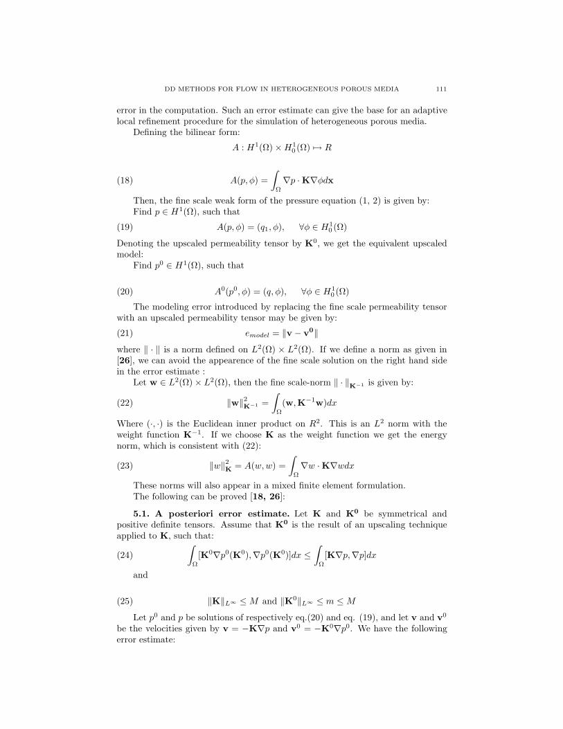
The assumption (24) states that the dissipation in the problem is constant ordecreasing during upscaling. Conservation of dissipation is one of the criteria usedfor judging the quality of an upscaling procedure see Section 4. The permeabilityrepresentation given in Section 2 is consistent with the assumptions given in thetheorem.

The aposteriori estimate of the modeling error is built on the results in [26].It is proved [26] that the upscaling based on this norm gives very good resultsand as noted, the estimate does not involve the fine scale solution. The error es-timate gives the basis for an adaptive upscaling technique. Together with domaindecomposition, it gives a strong modeling procedure. The following algorithm isconsistent with the hierarchical permeability representation given in Section 2:

Algorithm for an Adaptive Domain Decomposition SolutionSolve on scale 0. (Global coarse grid solve) This gives P 0

Ω and v0Ω

While( error ≥ tol and scale ≤ maxscale)Solve on all active local domains using the MRA representation.(After this step our data structure contains only inactive domains.)for(i = 1; i ≤ number of domains on this scale; i+ +)

if(local error ≥ tol)Generate four new active subdomains of this local domain.

end ifif(local error ≥ local error prev)

local error prev = local errorend if

end forerror = local error prev

end while( ... )

The separation of the domains into two classes, active and non-active, ensuresthat we do not waste time recomputing on domains which are not split up as wemove up in the hierarchy. Thus the iteration will just involve these four sub domains


Production

Ω

Injection

0

0.2

0.4

0.6

0.8

1 00.2

0.40.6

0.81

0

0.2

0.4

0.6

0.8

1

(a) (b)

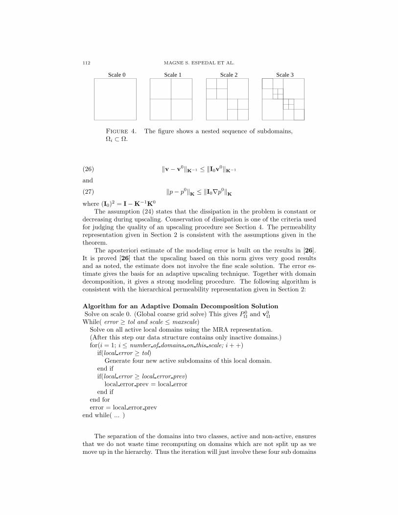
Figure 5. Experimental setting (a) and initial saturation profile (b).

if only one domain is refined. On the other hand if two neighboring domains arerefined, the iteration process will involve eight domains. Figure 4 shows a situationwhere all scales from scale 1 to scale 3 are present in the solution.

6. Numerical experiments

In this section we will present numerical experiments to demonstrate the effectof the error estimate and the “high-cut” upscaling technique. The computationswill be based on the permeability data given by Figure 3. All experiments are basedon the “quarter of a fivespot” problem. Our computational domain will be the unitsquare. Figure 5 shows a typical configuration along with the initial saturationprofile.

6.1. Reference Solution. The main objective of the experiment is to betterunderstand the behavior of the error estimate in theorem (5.1) together with domaindecomposition methods, based on local solvers [18]. We define the effectivityindices, ηK, [28], measuring the quality of the error prediction as:

ηK =‖I0v0‖2K−1

‖v0 − v‖2K−1

(28)

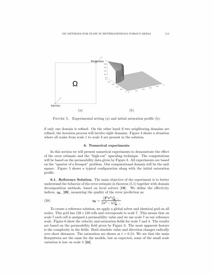
To create a reference solution, we apply a global solver and identical grid on allscales. This grid has 128×128 cells and corresponds to scale 7. This means that onscale 7 each cell is assigned a permeability value and we use scale 7 as our referencescale. Figure 6 show the velocity and saturation fields for scale 7 and 4. The resultsare based on the permeability field given by Figure 3. The most apparent featureis the complexity in the fields. Both absolute value and direction changes radicallyover short distances. The saturation are shown at t = 0.14. We see that the mainflowpattern are the same for the models, but as expected, some of the small scalevariation is lost on scale 4 [24].


0 10

1

X−Axis

Y−

Axi

s

0 10

1

X−AxisY

−A

xis

(a) Velocity field for Scale 7 (b) Velocity field for Scale 4

0 10

1

saturation at time=0.14

X−Axis

Y−A

xis

−0.00278

0.098

0.199

0.3

0.4

0.501

0.602

0.703

0.804

0.905

1.01

0 10

1


X−Axis

Y−A

xis

−0.00192

0.0983

0.198

0.299

0.399

0.499

0.599

0.699

0.8

0.9

1

(c) Saturation field for Scale 7 (d) Saturation field for Scale 4

Figure 6. The figure shows the velocity and saturation fieldsfor a highcut upscaling with global solvers. Figure (a) and (c)represent the reference solution. Scale 7 → 128 × 128 cells andscale 4 → 16× 16 cells.


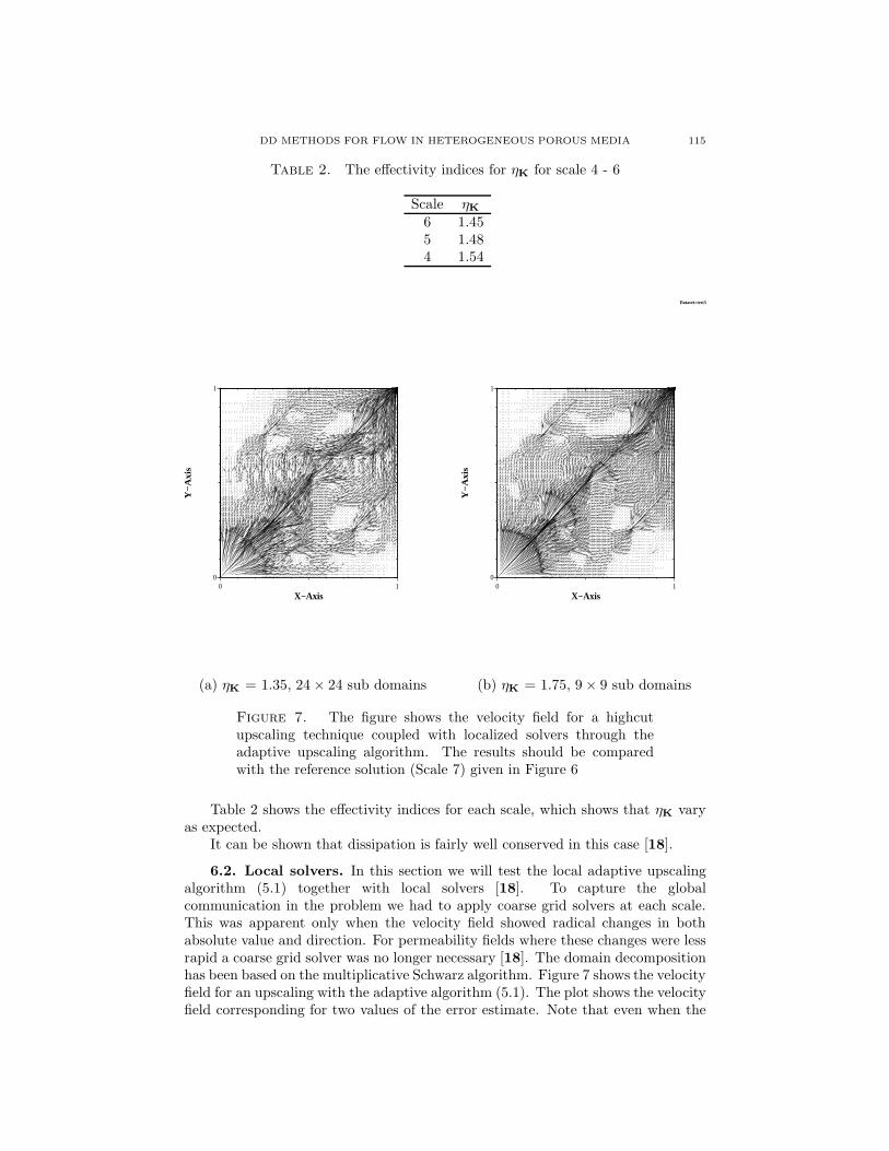
Table 2. The effectivity indices for ηK for scale 4 - 6

Scale ηK

6 1.455 1.484 1.54

0 10

1

X−Axis

Y−

Axi

s

0 10

1

X−Axis

Y−

Axi

s

Dataset=test3

(a) ηK = 1.35, 24× 24 sub domains (b) ηK = 1.75, 9× 9 sub domains

Figure 7. The figure shows the velocity field for a highcutupscaling technique coupled with localized solvers through theadaptive upscaling algorithm. The results should be comparedwith the reference solution (Scale 7) given in Figure 6

Table 2 shows the effectivity indices for each scale, which shows that ηK varyas expected.

It can be shown that dissipation is fairly well conserved in this case [18].

6.2. Local solvers. In this section we will test the local adaptive upscalingalgorithm (5.1) together with local solvers [18]. To capture the globalcommunication in the problem we had to apply coarse grid solvers at each scale.This was apparent only when the velocity field showed radical changes in bothabsolute value and direction. For permeability fields where these changes were lessrapid a coarse grid solver was no longer necessary [18]. The domain decompositionhas been based on the multiplicative Schwarz algorithm. Figure 7 shows the velocityfield for an upscaling with the adaptive algorithm (5.1). The plot shows the velocityfield corresponding for two values of the error estimate. Note that even when the


Injector

producer

K 2K

Ω Ω21

1

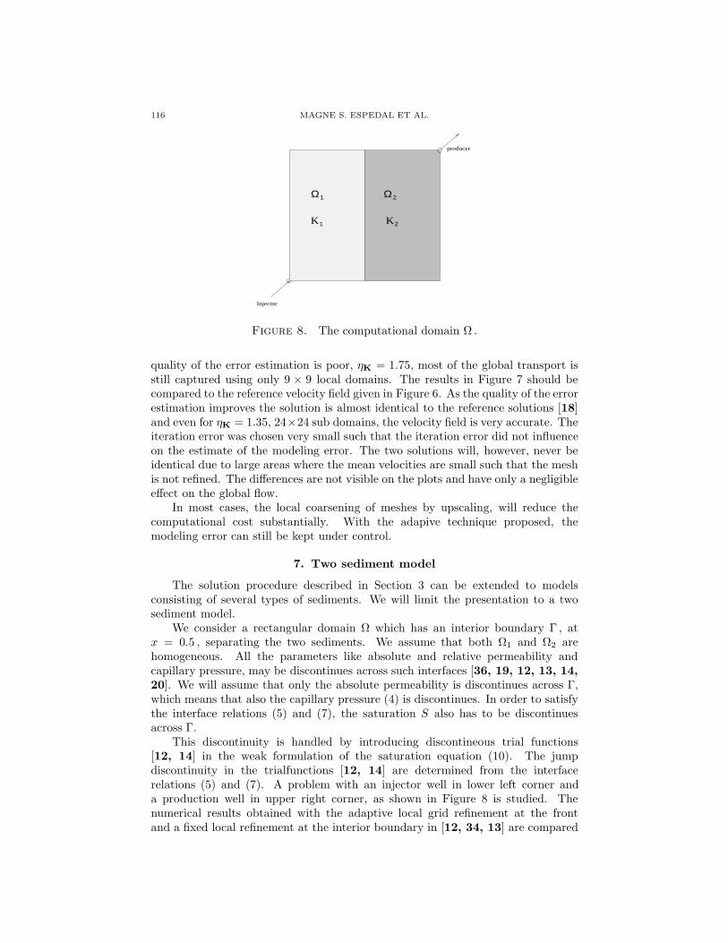
Figure 8. The computational domain Ω .

quality of the error estimation is poor, ηK = 1.75, most of the global transport isstill captured using only 9 × 9 local domains. The results in Figure 7 should becompared to the reference velocity field given in Figure 6. As the quality of the errorestimation improves the solution is almost identical to the reference solutions [18]and even for ηK = 1.35, 24×24 sub domains, the velocity field is very accurate. Theiteration error was chosen very small such that the iteration error did not influenceon the estimate of the modeling error. The two solutions will, however, never beidentical due to large areas where the mean velocities are small such that the meshis not refined. The differences are not visible on the plots and have only a negligibleeffect on the global flow.

In most cases, the local coarsening of meshes by upscaling, will reduce thecomputational cost substantially. With the adapive technique proposed, themodeling error can still be kept under control.

7. Two sediment model

The solution procedure described in Section 3 can be extended to modelsconsisting of several types of sediments. We will limit the presentation to a twosediment model.

We consider a rectangular domain Ω which has an interior boundary Γ , atx = 0.5 , separating the two sediments. We assume that both Ω1 and Ω2 arehomogeneous. All the parameters like absolute and relative permeability andcapillary pressure, may be discontinues across such interfaces [36, 19, 12, 13, 14,20]. We will assume that only the absolute permeability is discontinues across Γ,which means that also the capillary pressure (4) is discontinues. In order to satisfythe interface relations (5) and (7), the saturation S also has to be discontinuesacross Γ.

This discontinuity is handled by introducing discontineous trial functions[12, 14] in the weak formulation of the saturation equation (10). The jumpdiscontinuity in the trialfunctions [12, 14] are determined from the interfacerelations (5) and (7). A problem with an injector well in lower left corner anda production well in upper right corner, as shown in Figure 8 is studied. Thenumerical results obtained with the adaptive local grid refinement at the frontand a fixed local refinement at the interior boundary in [12, 34, 13] are compared


Table 3. Time and well data for the test cases.

Parameter value Decriptiondt 0.001 time stept [0,48] time intervallinj rate 0.2 injection rateprod rate -0.2 production rate

Table 4. The permeability fields defining test cases a and b.

case: K(Ω1) K(Ω2)a 1.0 0.1b 0.1 1.0

with equivalent results computed on a uniform global mesh. The local refinement isobtained by domain decomposition methods described in Section 3. The agreementbetween the two approaches is very good.

We choose the same type of initial condition for the saturation as given inFigure 5. This represents an established front, located away from the injectionwell.

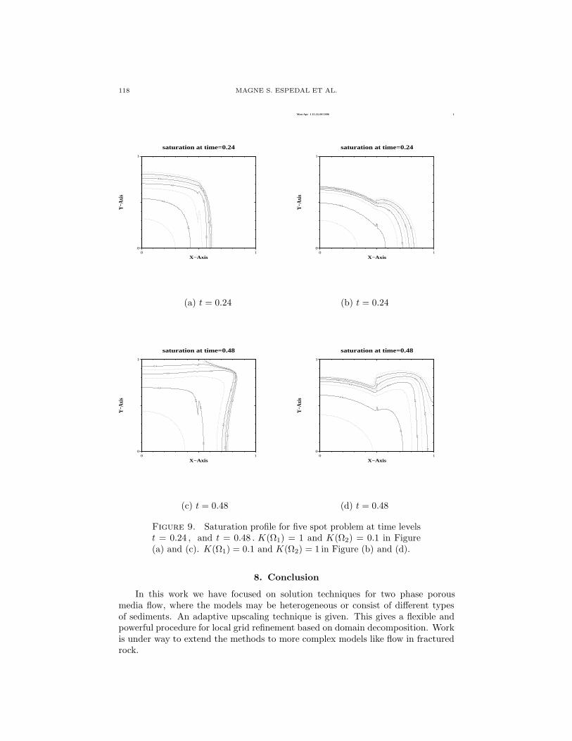
Saturation solutions will be shown at four time levels, t = 0.24 , and t = 0.48 .Input data are given in Table 3 and Table 4, while the injection and productionrates are given in Table 3 together with the time parameters.

Figure 9 gives computed saturations for the test cases a and b in Table 4. InFigure 9 (a) and (c) (Testcase a) water is injected in a high permeability sedimentand oil is produced in a low permeable sediment. In Figure 9 (b) and (d) (Testcaseb) water is injected in a low permeable sediment, and oil is produced in a highpermeable sediment.

The total Darcy velocity and the capillary diffusion depend on the permeabilityfield K. The effects of different permeabilities and capillary forces in the two regionsΩ1 and Ω2 combined with the effect of the boundary conditions (5), (7), are clearlyseen in Figure 9 (a) - (d) . The saturation jump at the internal boundary is positivefor testcase a and negative for testcase b [12, 14].

We observe that the saturation front is more smeared in the high permeableregion than in the low permeable region, consistent with the magnitude of thediffusion term as given in Figure 1.

As noted, the results shown are computed both with uniform grids and withlocal refinement based on domain decomposition [12]. The grid is adaptively refinedat the saturation fronts [8, 12] and at the internal boundary Γ. Except for smallinterpolation effects at the boundary between the coarse and the refined meshes,the results are similar.

The results are extended to models where both absolute and relativepermeability and capillary pressure are given by different functional form in thetwo sediments [12, 14]. Work is under way to extend the models to heterogeneousmultisediment models and models with fractures. The local refinement of meshesat interfaces and saturation fronts or the local coarsening of meshes by upscaling,will reduce the computational cost substantially.


0 10

1


X−Axis

Y−Ax

is

0.2

0.2

0.2

0.4

0.4

0.4

0.6

0.60.6

0.8

0.8

Mon Apr 1 15:31:08 1996

0 10

1


X−Axis

Y−Ax

is

1

0.2

0.2

0.2

0.4

0.4

0.4

0.6

0.6

0.6

0.8

0.8

(a) t = 0.24 (b) t = 0.24

0 10

1


X−Axis

Y−Ax

is

0.2

0.2

0.2

0.4 0.4

0.4

0.4

0.4

0.60.6

0.6

0.6

0.8

0.8

0.80.8

0 10

1


X−Axis

Y−Ax

is

0.20.2 0.20.4

0.4

0.4

0.40.4

0.60.6

0.60.6

0.8

0.8

0.8

(c) t = 0.48 (d) t = 0.48

Figure 9. Saturation profile for five spot problem at time levelst = 0.24 , and t = 0.48 . K(Ω1) = 1 and K(Ω2) = 0.1 in Figure(a) and (c). K(Ω1) = 0.1 and K(Ω2) = 1 in Figure (b) and (d).

8. Conclusion

In this work we have focused on solution techniques for two phase porousmedia flow, where the models may be heterogeneous or consist of different typesof sediments. An adaptive upscaling technique is given. This gives a flexible andpowerful procedure for local grid refinement based on domain decomposition. Workis under way to extend the methods to more complex models like flow in fracturedrock.


References

1. B. Amazine, A Bourgeat, and J. V. Koebbe, Numerical simulation and homogenization ofdiphasic flow in heterogeneous reservoirs, Proceedings II European conf. on Math. in OilRecovery (Arle, France) (O. Guillon D. Guerillot, ed.), 1990.

2. O. Axelsson and V.A. Barker, Finite element solution of boundary value problems, AcademicPress, London, 1984.

3. J.W. Barrett and K.W. Morton, Approximate symmetrization and Petrov-Galerkin methodsfor diffusion-convection problems, Computer Methods in Applied Mechanics and Engineering45 (1984), 97–122.

4. Ø. Bøe, Finite-element methods for porous media flow, Ph.D. thesis, Department of AppliedMathematics, University of Bergen, Norway, 1990.

5. G. Chavent and J.Jaffre, Mathematical models and finite elements for reservoir simulation,North-Holland, Amsterdam, 1987.

6. C. K. Chu, An introduction to wavelets, Academic Press, Boston, 1992.7. G. Dagan, Flow and transport in porous formations, Springer-Verlag, Berlin-Heidelberg, 1989.8. H.K. Dahle, M.S. Espedal, and O. Sævareid, Characteristic, local grid refinement techniques

for reservoir flow problems, Int. Journal for Numerical Methods in Engineering 34 (1992),1051–1069.

9. I. Daubechies, Ten lectures on wavelets, Conf. Ser.Appl. Math. SIAM, Philadelphia, 1992.10. J. Douglas, Jr. and T.F. Russell, Numerical methods for convection-dominated diffusion

problems based on combining the method of characteristics with finite element or finitedifference procedures, SIAM Journal on Numerical Analysis 19 (1982), 871–885.

11. L. J. Durlofsky and E. Y. Chang, Effective permeability of heterogeneous reservoir regions,

Proceedings II European conf. on Math. in Oil Recovery (Arle, France) (O. GuillonD. Guerillot, ed.), 1990.

12. B. G. Ersland, On numerical methods for including the effect of capillary presure forces ontwo-phase, immmiscible flow in a layered porous media, Ph.D. thesis, Department of AppliedMathematics, University of Bergen, Norway, 1996.

13. B. G. Ersland and M. S. Espedal, Domain decomposition method for heterogeneous reservoirflow, Proceedings Eight International Conference on Domain Decomposition Methods, Beijing,1995 (London) (R. Glowinski, J. Periaux, Z-C. Shi, and O. Widlund, eds.), J.Wiley, 1997.

14. M. S. Espedal, B. G. Ersland, K. Hersvik, and R. Nybø, Domain decomposition based methodsfor flow in a porous media with internal boundaries, Submitted to: Computational Geoscience,1997.

15. M. S. Espedal and R.E. Ewing, Characteristic Petrov-Galerkin subdomain methods for two-phase immiscible flow, Computer Methods in Applied Mechanics and Engineering 64 (1987),113–135.

16. J. Frøyen and M. S. Espedal, A 3D parallel reservoir simulator, Proceedings V Europeanconf. on Math. in Oil Recovery (Leoben,Austria) (M. Kriebernegg E. Heinemann, ed.), 1996.

17. R. Hansen and M. S. Espedal, On the numerical solution of nonlinear flow models with gravity,Int. J. for Num. Meth. in Eng. 38 (1995), 2017–2032.

18. K. Hersvik and M. S. Espedal, An adaptive upscaling technique based on an a-priori errorestimate, Submitted to: Computational Geoscience, 1997.

19. J. Jaffre, Flux calculation at the interface between two rock types for two-phase flow in porousmedia, Transport in Porous Media 21 (1995), 195–207.

20. J. Jaffre and J. Roberts, Flux calculation at the interface between two rock types for two-phaseflow in porous media, Proceedings Tenth International Conference on Domain DecompositionMethods, Boulder, (1997).

21. K. Hvistendahl Karlsen, K. Brusdal, H. K. Dahle, S. Evje, and K. A. Lie, The correctedoperator splitting approach applied to nonlinear advection-diffusion problem, ComputerMethods in Applied Mechanics and Engineering (1998), To appear.

22. P. R. King, The use of renormalization for calculating effective permebility, Transport inPorous Media 4 (1989), 37–58.

23. T. F. M. Kortekaas, Water/oil displacement characteristics in crossbedded reservoir zones,Society of Petroleum Engineers Journal (1985), 917–926.

24. P. Langlo and M. S. Espedal, Macrodispersion for two-phase immiscible flow in porous media,Advances in Water Resources 17 (1994), 297–316.


25. K. W. Morton, Numerical solution of convection-diffusion problems, Applied Mathematicsand Mathematical Computation, 12, Chapman & Hall, London, 1996.

26. B. F. Nielsen and A. Tveito, An upscaling method for one-phase flow in heterogenousreservoirs; a weighted output least squares approach, Preprint, Dep. of informatics, Univ.of Oslo, Norway, 1996.

27. S. Nilsen and M. S. Espedal, Upscaling based on piecewise bilinear approximation of thepermeability field, Transport in Porous Media 23 (1996), 125–134.

28. J. T. Oden, T. Zohdi, and J. R. Cho, Hierarchical modelling, a posteriori error estimate andadaptive methods in computational mechanics, Proceedings Comp. Meth. in Applied Sciences(London) (J. A. Desideri et.al., ed.), J. Wiley, 1996, pp. 37–47.

29. R. Rannacher and G. H. Zhou., Analysis of a domain splitting method for nonstationaryconvection-diffuion problems, East-West J. Numer. math. 2 (1994), 151–174.

30. Y. Rubin, Stochastic modeling of macrodispersion in heterogeneous poros media, WaterResources Res. 26 (1991), 133–141.

31. O. Sævareid, On local grid refinement techniques for reservoir flow problems, Ph.D. thesis,Department of Applied Mathematics, University of Bergen, Norway, 1990.

32. B. Smith, P. Bjørstad, and W. Gropp, Domain decomposition, Cambridge University Press,Camebridge, 1996.

33. X. C. Tai and M. S. Espedal, Space decomposition methods and application to linear andnonlinear elliptic problems, Int. J. for Num. Meth. in Eng. (1998), To appear.

34. X. C. Tai, O. W. Johansen, H. K. Dahle, and M. S. Espedal, A characteristic domain splittingmethod for time-dependent convection diffusion problems, Proceedings Eight InternationalConference on Domain Decomposition Methods, Beijing, 1995 (London) (R. Glowinski,J. Periaux, Z-C. Shi, and O. Widlund, eds.), J.Wiley, 1997.

35. T.Bu and L.B. Haøy, On the importance of correct inclusion of capillary pressure in reservoirsimulation, Proceedings European IOR - Symposium, 1995.

36. C. J. van Duijn, J. Molenaar, and M. J. de Neef, The effect of the capillary forces on immiscibletwo-phase flow in heterogenous porous media, Transport in Porous Media 21 (1995), 71–93.

Department of Mathematics, University of Bergen, N-5008 Bergen, Norway

E-mail address: [email protected]

Department of Mathematics, University of Bergen, N-5008 Bergen, Norway


Statoil a.s., N-5020 Bergen, Norway


Domain Decomposition Methods for Flow in … Mathematics Volume 218, 1998 Domain Decomposition...

Documents

Transcript of Domain Decomposition Methods for Flow in … Mathematics Volume 218, 1998 Domain Decomposition...