Is God a geometer or an analyst?

Dmitri Vassiliev

23 November 2012

UCL ADM Maths Society

1

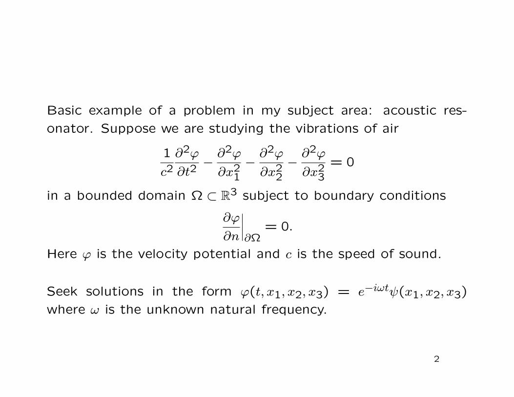
Basic example of a problem in my subject area: acoustic res-

onator. Suppose we are studying the vibrations of air

1

c2∂2ϕ

∂t2−∂2ϕ

∂x21−∂2ϕ

∂x22−∂2ϕ

∂x23

= 0

in a bounded domain Ω ⊂ R3 subject to boundary conditions

∂ϕ

∂n

∣∣∣∣∂Ω

= 0.

Here ϕ is the velocity potential and c is the speed of sound.

Seek solutions in the form ϕ(t, x1, x2, x3) = e−iωtψ(x1, x2, x3)

where ω is the unknown natural frequency.

2

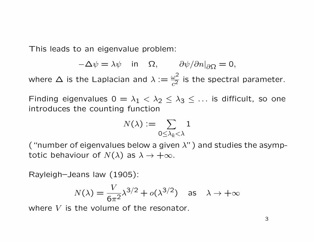
This leads to an eigenvalue problem:

−∆ψ = λψ in Ω, ∂ψ/∂n|∂Ω = 0,

where ∆ is the Laplacian and λ := ω2

c2is the spectral parameter.

Finding eigenvalues 0 = λ1 < λ2 ≤ λ3 ≤ . . . is difficult, so oneintroduces the counting function

N(λ) :=∑

0≤λk<λ1

(“number of eigenvalues below a given λ”) and studies the asymp-totic behaviour of N(λ) as λ→ +∞.

Rayleigh–Jeans law (1905):

N(λ) =V

6π2λ3/2 + o(λ3/2) as λ→ +∞

where V is the volume of the resonator.3

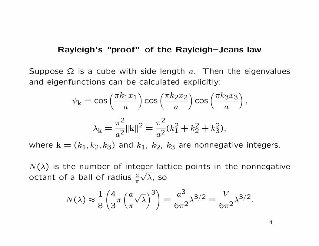
Rayleigh’s “proof” of the Rayleigh–Jeans law

Suppose Ω is a cube with side length a. Then the eigenvalues

and eigenfunctions can be calculated explicitly:

ψk = cos(πk1x1

a

)cos

(πk2x2

a

)cos

(πk3x3

a

),

λk =π2

a2‖k‖2 =

π2

a2(k2

1 + k22 + k2

3),

where k = (k1, k2, k3) and k1, k2, k3 are nonnegative integers.

N(λ) is the number of integer lattice points in the nonnegative

octant of a ball of radius aπ

√λ, so

N(λ) ≈1

8

(4

3π

(a

π

√λ

)3)

=a3

6π2λ3/2 =

V

6π2λ3/2.

4

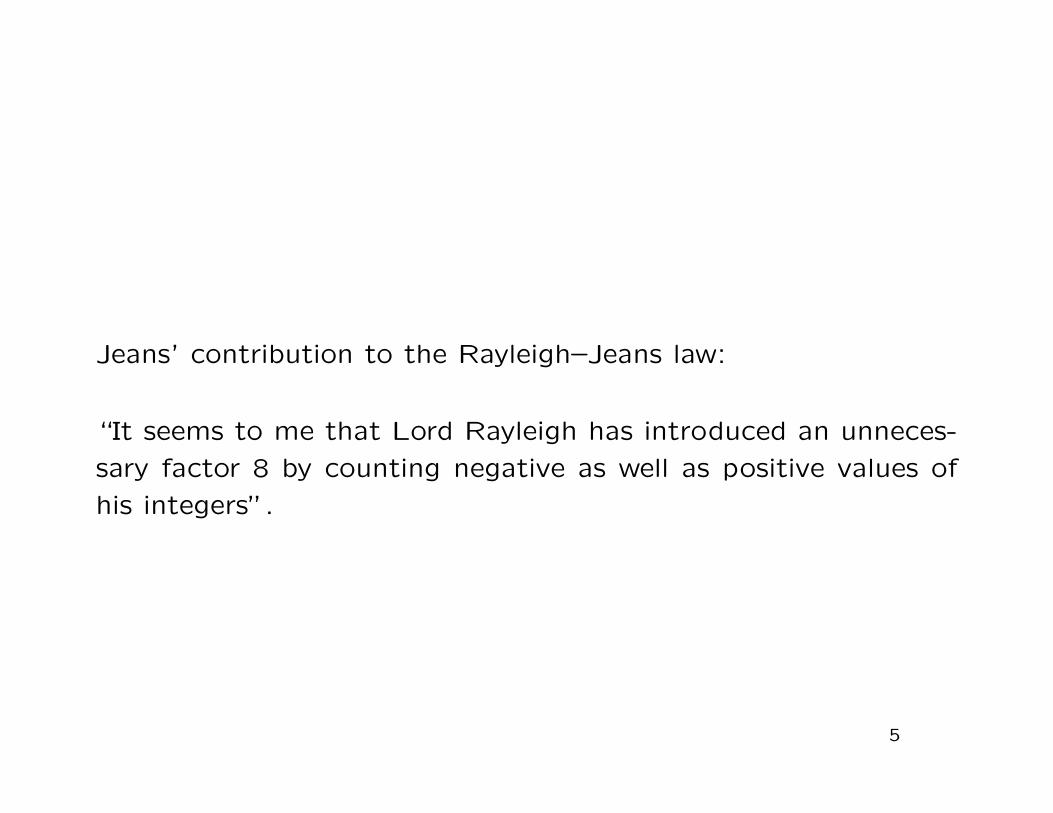
Jeans’ contribution to the Rayleigh–Jeans law:

“It seems to me that Lord Rayleigh has introduced an unneces-

sary factor 8 by counting negative as well as positive values of

his integers”.

5

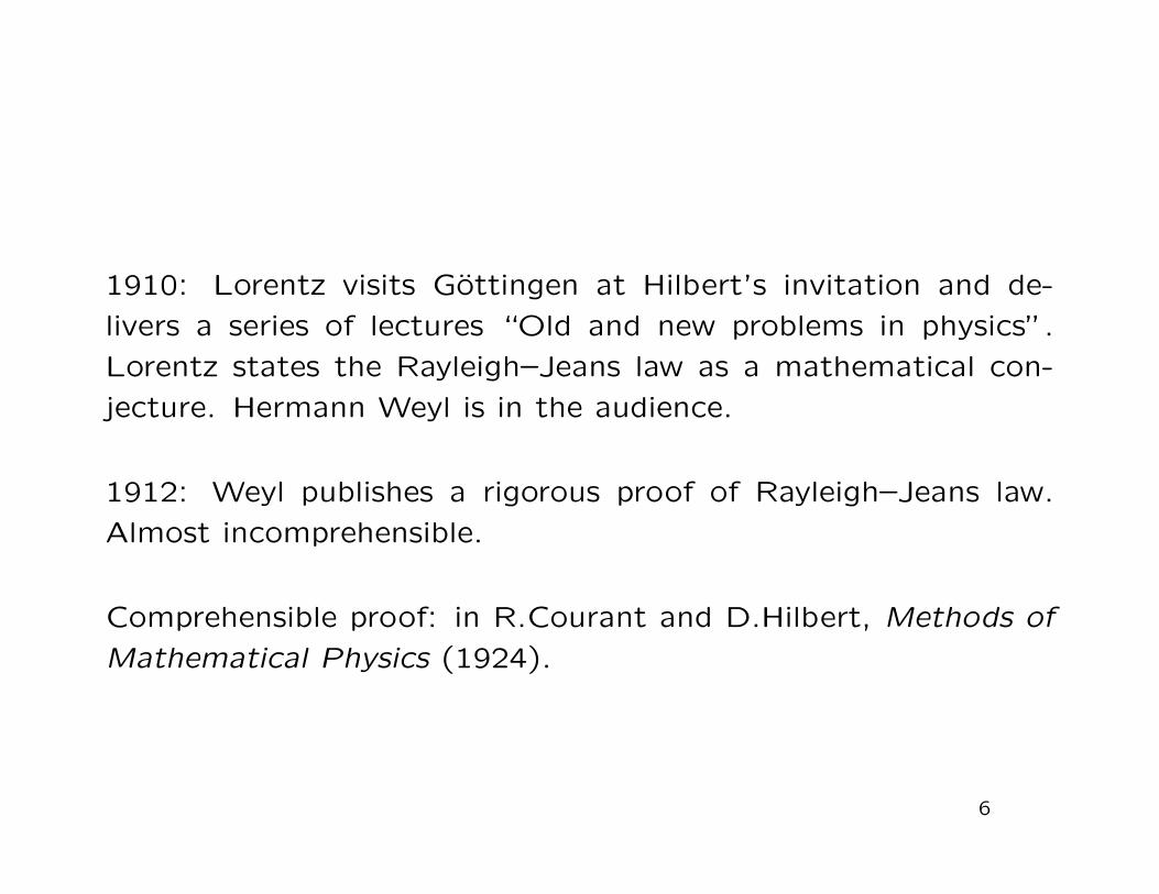
1910: Lorentz visits Gottingen at Hilbert’s invitation and de-

livers a series of lectures “Old and new problems in physics”.

Lorentz states the Rayleigh–Jeans law as a mathematical con-

jecture. Hermann Weyl is in the audience.

1912: Weyl publishes a rigorous proof of Rayleigh–Jeans law.

Almost incomprehensible.

Comprehensible proof: in R.Courant and D.Hilbert, Methods of

Mathematical Physics (1924).

6

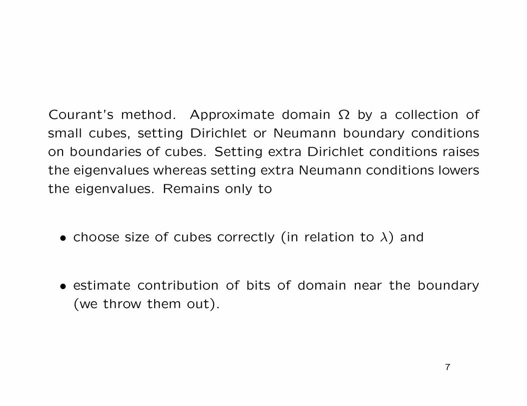
Courant’s method. Approximate domain Ω by a collection of

small cubes, setting Dirichlet or Neumann boundary conditions

on boundaries of cubes. Setting extra Dirichlet conditions raises

the eigenvalues whereas setting extra Neumann conditions lowers

the eigenvalues. Remains only to

• choose size of cubes correctly (in relation to λ) and

• estimate contribution of bits of domain near the boundary

(we throw them out).

7

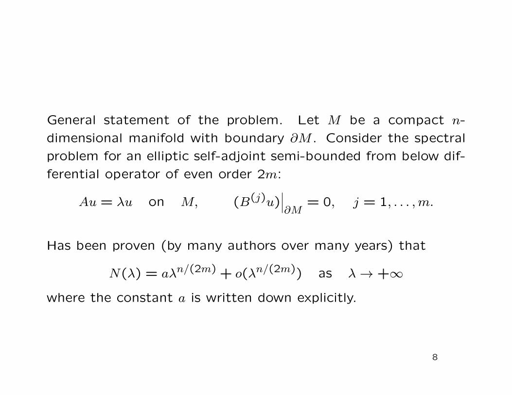
General statement of the problem. Let M be a compact n-

dimensional manifold with boundary ∂M . Consider the spectral

problem for an elliptic self-adjoint semi-bounded from below dif-

ferential operator of even order 2m:

Au = λu on M, (B(j)u)∣∣∣∂M

= 0, j = 1, . . . ,m.

Has been proven (by many authors over many years) that

N(λ) = aλn/(2m) + o(λn/(2m)) as λ→ +∞

where the constant a is written down explicitly.

8

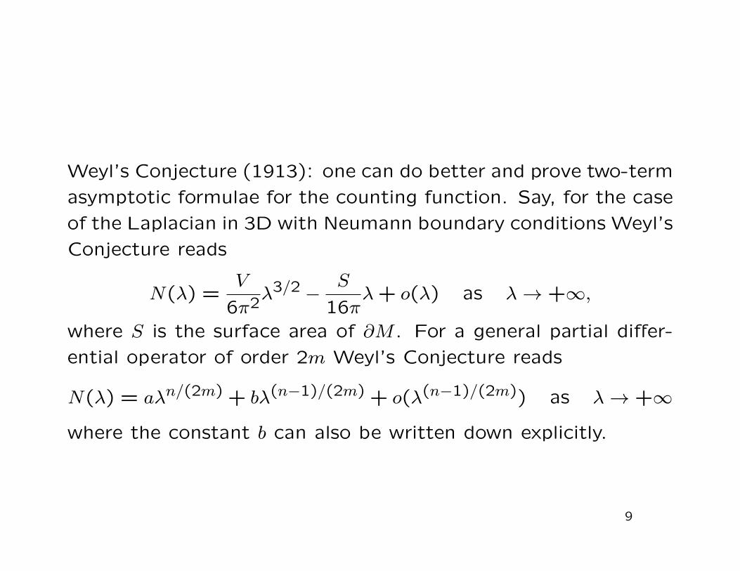
Weyl’s Conjecture (1913): one can do better and prove two-term

asymptotic formulae for the counting function. Say, for the case

of the Laplacian in 3D with Neumann boundary conditions Weyl’s

Conjecture reads

N(λ) =V

6π2λ3/2 −

S

16πλ+ o(λ) as λ→ +∞,

where S is the surface area of ∂M . For a general partial differ-

ential operator of order 2m Weyl’s Conjecture reads

N(λ) = aλn/(2m) + bλ(n−1)/(2m) + o(λ(n−1)/(2m)) as λ→ +∞

where the constant b can also be written down explicitly.

9

For the case of a second order operator Weyl’s Conjecture was

proved by V.Ivrii in 1980. I proved it for operators of arbitrary

order in 1984.

My main research publication:

Yu.Safarov and D.Vassiliev, The asymptotic distribution of eigen-

values of partial differential operators, American Mathematical

Society, 1997 (hardcover), 1998 (softcover).

“In the reviewer’s opinion, this book is indispensable for seri-

ous students of spectral asymptotics”. Lars Hormander for the

Bulletin of the London Mathematical Society.

10

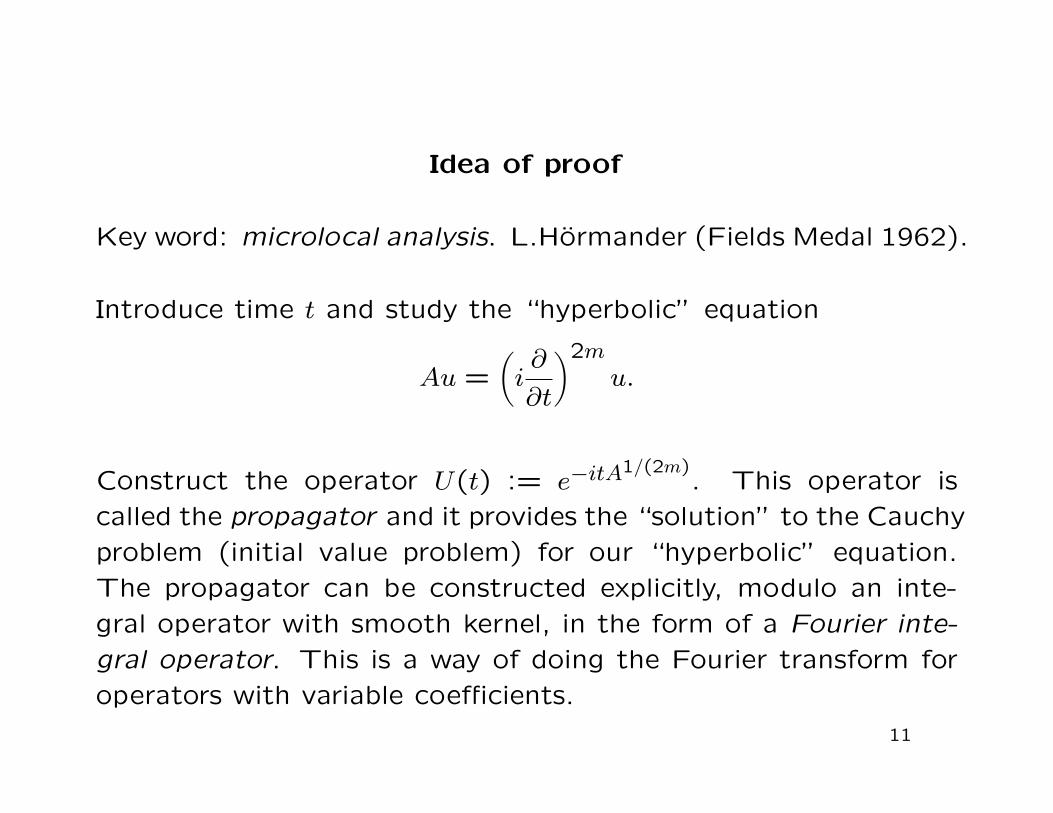
Idea of proof

Key word: microlocal analysis. L.Hormander (Fields Medal 1962).

Introduce time t and study the “hyperbolic” equation

Au =(i∂

∂t

)2mu.

Construct the operator U(t) := e−itA1/(2m)

. This operator is

called the propagator and it provides the “solution” to the Cauchy

problem (initial value problem) for our “hyperbolic” equation.

The propagator can be constructed explicitly, modulo an inte-

gral operator with smooth kernel, in the form of a Fourier inte-

gral operator. This is a way of doing the Fourier transform for

operators with variable coefficients.

11

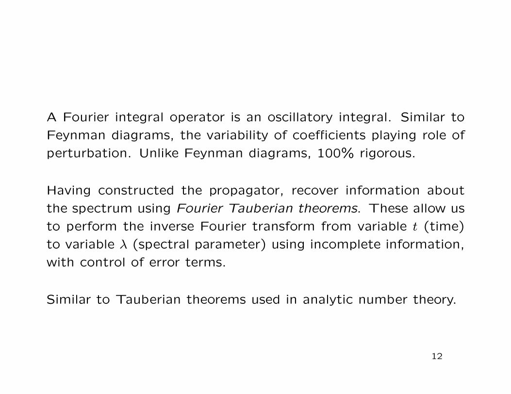
A Fourier integral operator is an oscillatory integral. Similar to

Feynman diagrams, the variability of coefficients playing role of

perturbation. Unlike Feynman diagrams, 100% rigorous.

Having constructed the propagator, recover information about

the spectrum using Fourier Tauberian theorems. These allow us

to perform the inverse Fourier transform from variable t (time)

to variable λ (spectral parameter) using incomplete information,

with control of error terms.

Similar to Tauberian theorems used in analytic number theory.

12

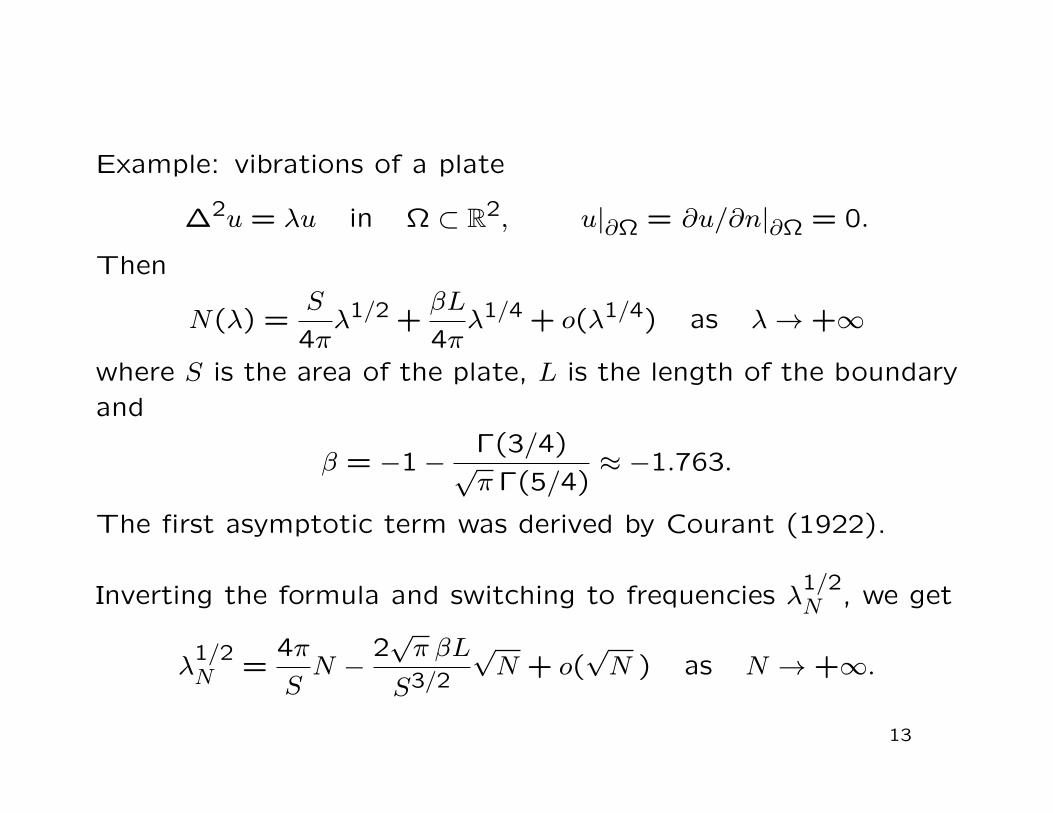
Example: vibrations of a plate

∆2u = λu in Ω ⊂ R2, u|∂Ω = ∂u/∂n|∂Ω = 0.

Then

N(λ) =S

4πλ1/2 +

βL

4πλ1/4 + o(λ1/4) as λ→ +∞

where S is the area of the plate, L is the length of the boundaryand

β = −1−Γ(3/4)√π Γ(5/4)

≈ −1.763.

The first asymptotic term was derived by Courant (1922).

Inverting the formula and switching to frequencies λ1/2N , we get

λ1/2N =

4π

SN −

2√π βL

S3/2

√N + o(

√N ) as N → +∞.

13

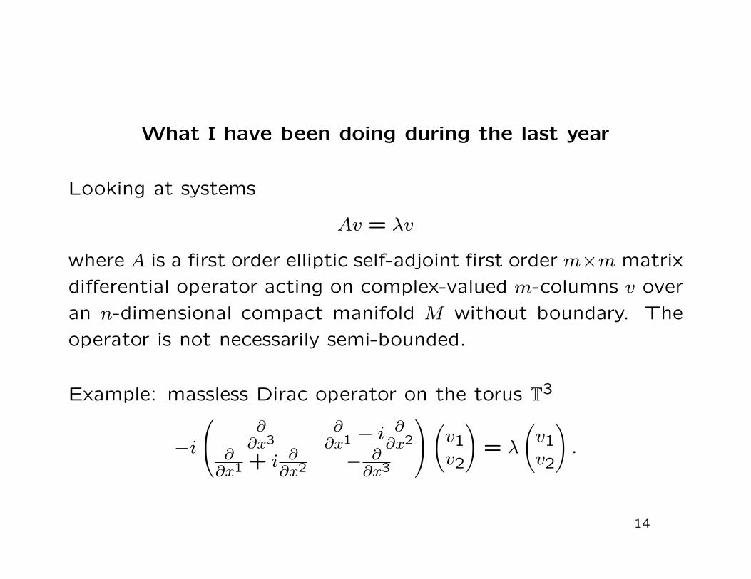
What I have been doing during the last year

Looking at systems

Av = λv

where A is a first order elliptic self-adjoint first order m×m matrix

differential operator acting on complex-valued m-columns v over

an n-dimensional compact manifold M without boundary. The

operator is not necessarily semi-bounded.

Example: massless Dirac operator on the torus T3

−i

∂∂x3

∂∂x1 − i ∂

∂x2∂∂x1 + i ∂

∂x2 − ∂∂x3

(v1v2

)= λ

(v1v2

).

14

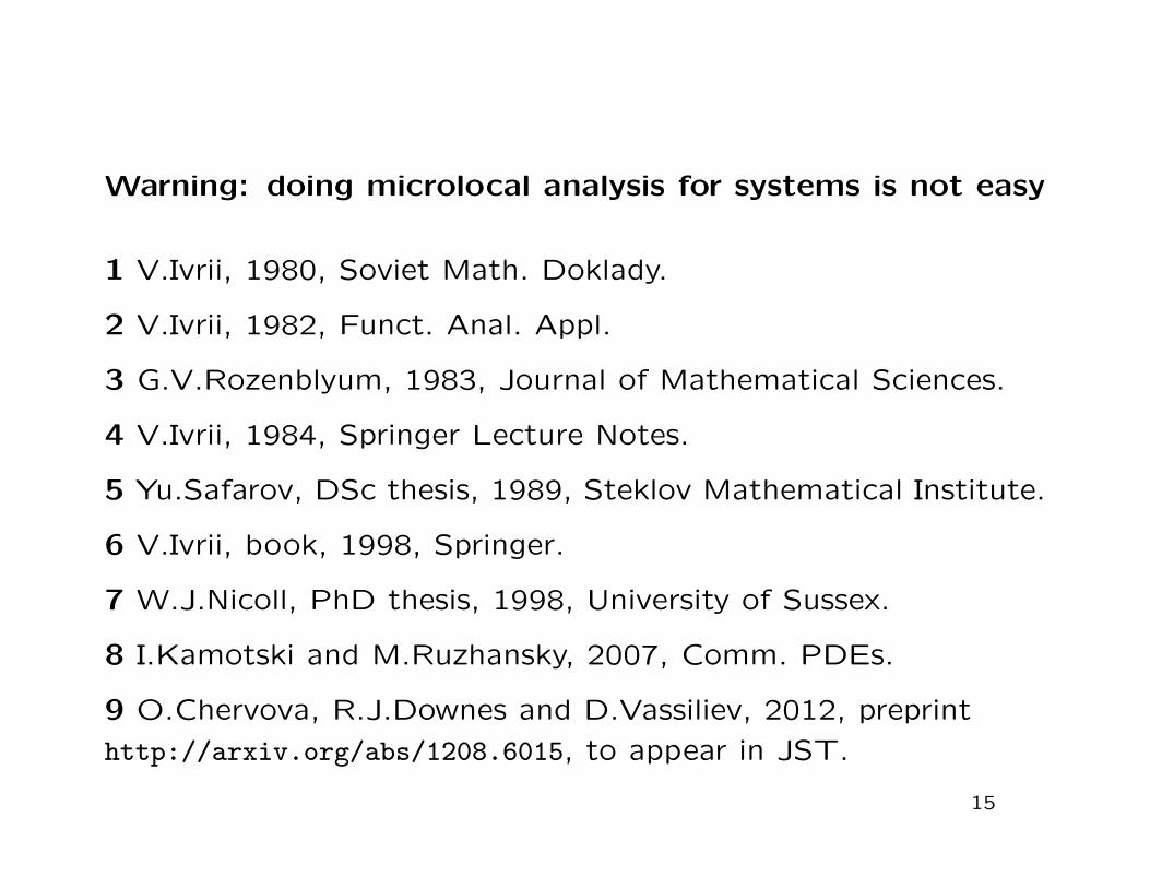
Warning: doing microlocal analysis for systems is not easy

1 V.Ivrii, 1980, Soviet Math. Doklady.

2 V.Ivrii, 1982, Funct. Anal. Appl.

3 G.V.Rozenblyum, 1983, Journal of Mathematical Sciences.

4 V.Ivrii, 1984, Springer Lecture Notes.

5 Yu.Safarov, DSc thesis, 1989, Steklov Mathematical Institute.

6 V.Ivrii, book, 1998, Springer.

7 W.J.Nicoll, PhD thesis, 1998, University of Sussex.

8 I.Kamotski and M.Ruzhansky, 2007, Comm. PDEs.

9 O.Chervova, R.J.Downes and D.Vassiliev, 2012, preprint

http://arxiv.org/abs/1208.6015, to appear in JST.

15

The circle group U(1)

U(1) = z ∈ C : |z| = 1.

Here the group operation is multiplication.

16

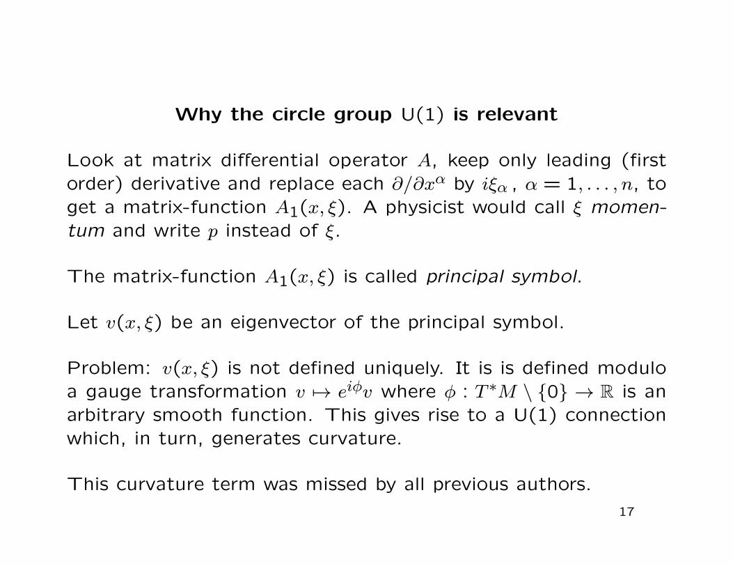
Why the circle group U(1) is relevant

Look at matrix differential operator A, keep only leading (firstorder) derivative and replace each ∂/∂xα by iξα , α = 1, . . . , n, toget a matrix-function A1(x, ξ). A physicist would call ξ momen-tum and write p instead of ξ.

The matrix-function A1(x, ξ) is called principal symbol.

Let v(x, ξ) be an eigenvector of the principal symbol.

Problem: v(x, ξ) is not defined uniquely. It is is defined moduloa gauge transformation v 7→ eiφv where φ : T ∗M \ 0 → R is anarbitrary smooth function. This gives rise to a U(1) connectionwhich, in turn, generates curvature.

This curvature term was missed by all previous authors.

17

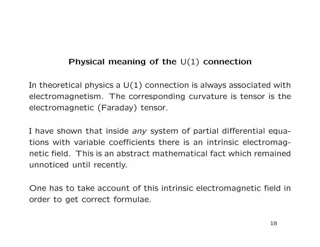
Physical meaning of the U(1) connection

In theoretical physics a U(1) connection is always associated with

electromagnetism. The corresponding curvature is tensor is the

electromagnetic (Faraday) tensor.

I have shown that inside any system of partial differential equa-

tions with variable coefficients there is an intrinsic electromag-

netic field. This is an abstract mathematical fact which remained

unnoticed until recently.

One has to take account of this intrinsic electromagnetic field in

order to get correct formulae.

18

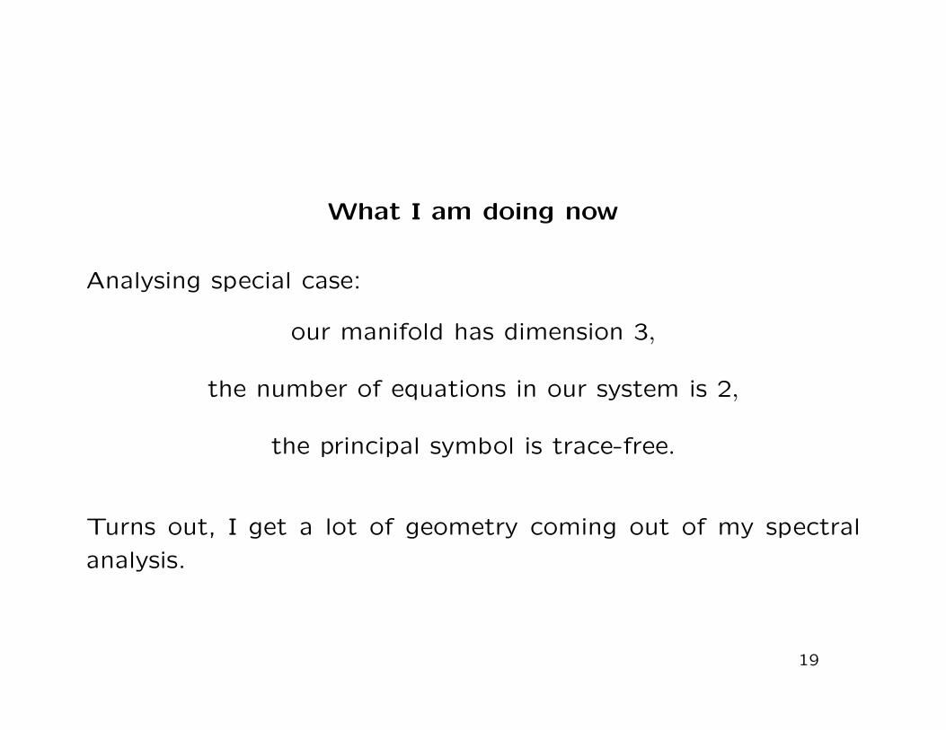
What I am doing now

Analysing special case:

our manifold has dimension 3,

the number of equations in our system is 2,

the principal symbol is trace-free.

Turns out, I get a lot of geometry coming out of my spectral

analysis.

19

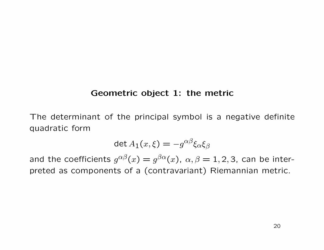
Geometric object 1: the metric

The determinant of the principal symbol is a negative definite

quadratic form

detA1(x, ξ) = −gαβξαξβand the coefficients gαβ(x) = gβα(x), α, β = 1,2,3, can be inter-

preted as components of a (contravariant) Riemannian metric.

20

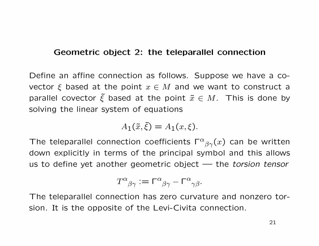
Geometric object 2: the teleparallel connection

Define an affine connection as follows. Suppose we have a co-

vector ξ based at the point x ∈ M and we want to construct a

parallel covector ξ based at the point x ∈ M . This is done by

solving the linear system of equations

A1(x, ξ) = A1(x, ξ).

The teleparallel connection coefficients Γαβγ(x) can be written

down explicitly in terms of the principal symbol and this allows

us to define yet another geometric object — the torsion tensor

Tαβγ := Γαβγ − Γαγβ.

The teleparallel connection has zero curvature and nonzero tor-

sion. It is the opposite of the Levi-Civita connection.

21

Geometric object 3: spinor field

Spinor = quaternion a + bi + cj + dk, where a, b, c, d ∈ R andi2 = j2 = k2 = ijk = −1.

Where does spinor come from? 2×2 trace-free Hermitian matrix-function A1(x, ξ) is not fully defined by its determinant (metric).Remaining degrees of freedom are described by a spinor.

Geometric object 4: massless Dirac action

Action = variational functional for corresponding diff. operator.

Turns out, the second asymptotic coefficient of the countingfunction has the geometric meaning of the massless Dirac action.

Bottom line: the differential geometry of spinors is encodedwithin the microlocal analysis of PDEs.

22

Four fundamental equations of theoretical physics

1 Maxwell’s equations. Describe electromagnetism and photons.

2 Dirac equation. Describes electrons and positrons.

3 Massless Dirac equation. Describes∗ neutrinos and antineutrinos.

4 Linearized Einstein field equations of general relativity. De-

scribe gravity.

All four contain the same physical constant — the speed of light.

∗OK, I know that neutrinos actually have a small mass.

23

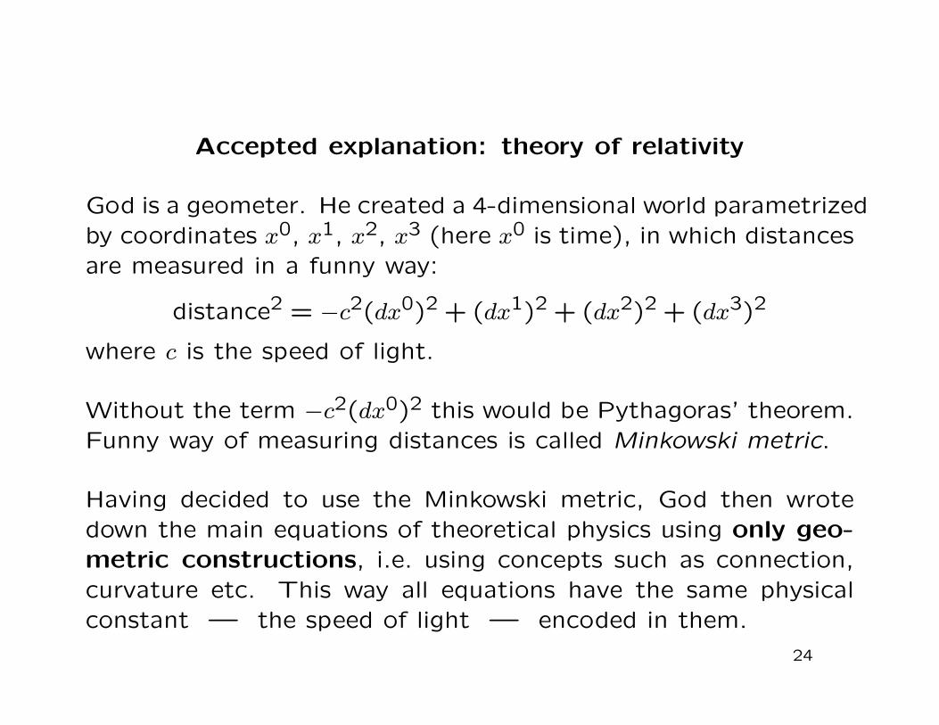
Accepted explanation: theory of relativity

God is a geometer. He created a 4-dimensional world parametrizedby coordinates x0, x1, x2, x3 (here x0 is time), in which distancesare measured in a funny way:

distance2 = −c2(dx0)2 + (dx1)2 + (dx2)2 + (dx3)2

where c is the speed of light.

Without the term −c2(dx0)2 this would be Pythagoras’ theorem.Funny way of measuring distances is called Minkowski metric.

Having decided to use the Minkowski metric, God then wrotedown the main equations of theoretical physics using only geo-metric constructions, i.e. using concepts such as connection,curvature etc. This way all equations have the same physicalconstant — the speed of light — encoded in them.

24

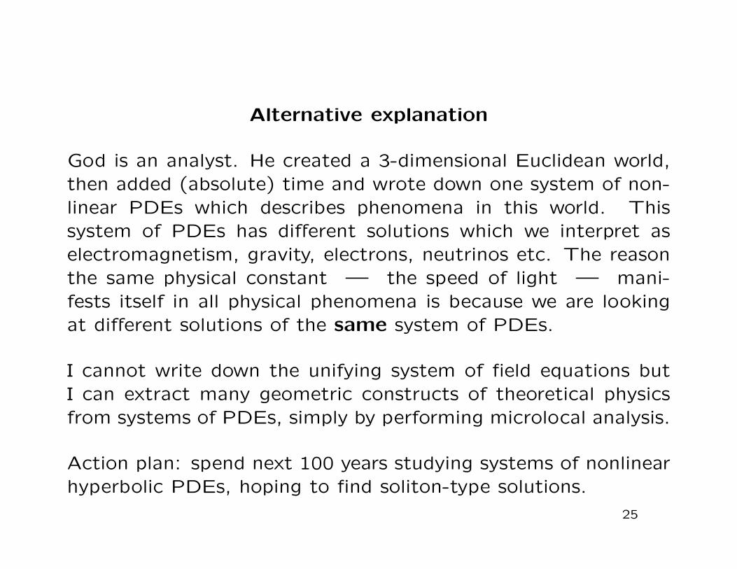
Alternative explanation

God is an analyst. He created a 3-dimensional Euclidean world,then added (absolute) time and wrote down one system of non-linear PDEs which describes phenomena in this world. Thissystem of PDEs has different solutions which we interpret aselectromagnetism, gravity, electrons, neutrinos etc. The reasonthe same physical constant — the speed of light — mani-fests itself in all physical phenomena is because we are lookingat different solutions of the same system of PDEs.

I cannot write down the unifying system of field equations butI can extract many geometric constructs of theoretical physicsfrom systems of PDEs, simply by performing microlocal analysis.

Action plan: spend next 100 years studying systems of nonlinearhyperbolic PDEs, hoping to find soliton-type solutions.

25

My PhD students who helped me a lot in recent years

Vedad Pasic

James Burnett

Olga Chervova

Rob Downes

26