Divide & Conquer - Boise State CScs.boisestate.edu/~cs521/slides/NewSlides/DivideConquer.pdf ·...
11
Divide & Conquer Algorithms
Transcript of Divide & Conquer - Boise State CScs.boisestate.edu/~cs521/slides/NewSlides/DivideConquer.pdf ·...
Divide&ConquerAlgorithms
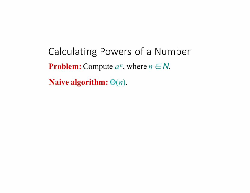
CalculatingPowersofa NumberProblem: Compute a n, where n ∈N.
Naive algorithm:Θ(n).
CalculatingPowersofa NumberProblem: Compute a n, where n ∈N.
Naive algorithm:Θ(n).
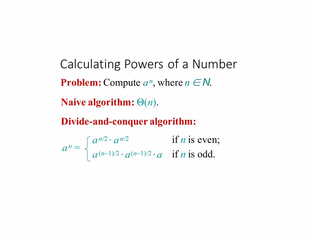
Divide-and-conquer algorithm:
a n =a n/2 ⋅ a n/2
a (n–1)/2 ⋅ a (n–1)/2 ⋅aif n is even; if n is odd.
CalculatingPowersofa NumberProblem: Compute a n, where n ∈N.
Naive algorithm:Θ(n).
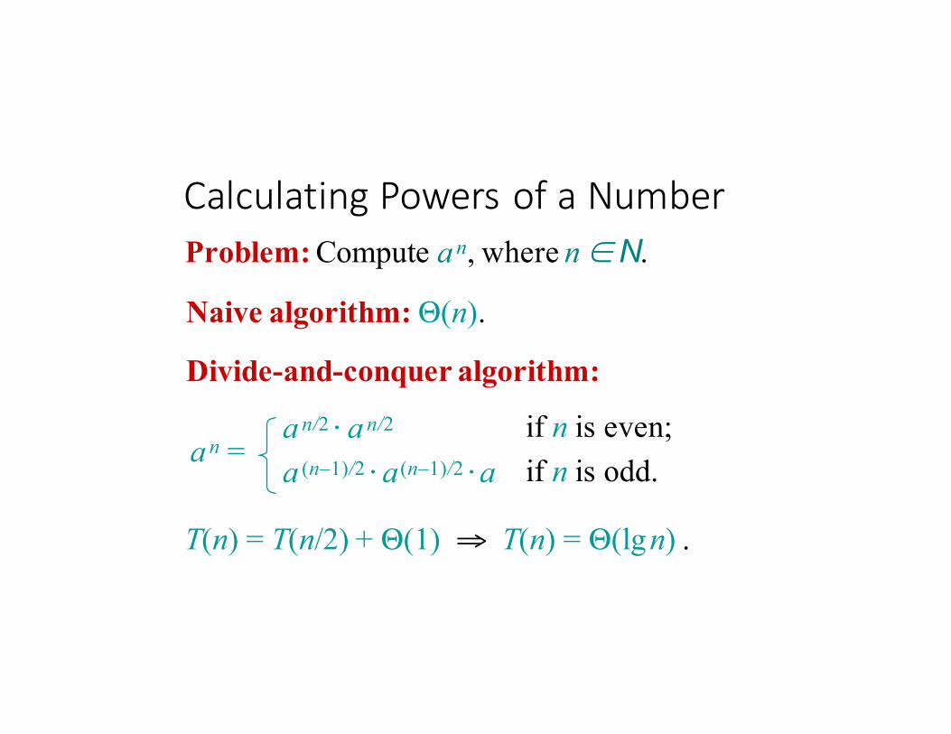
Divide-and-conquer algorithm:
a n =a n/2 ⋅ a n/2
a (n–1)/2 ⋅ a (n–1)/2 ⋅aif n is even; if n is odd.
T(n) = T(n/2) + Θ(1) ⇒ T(n) = Θ(lgn) .
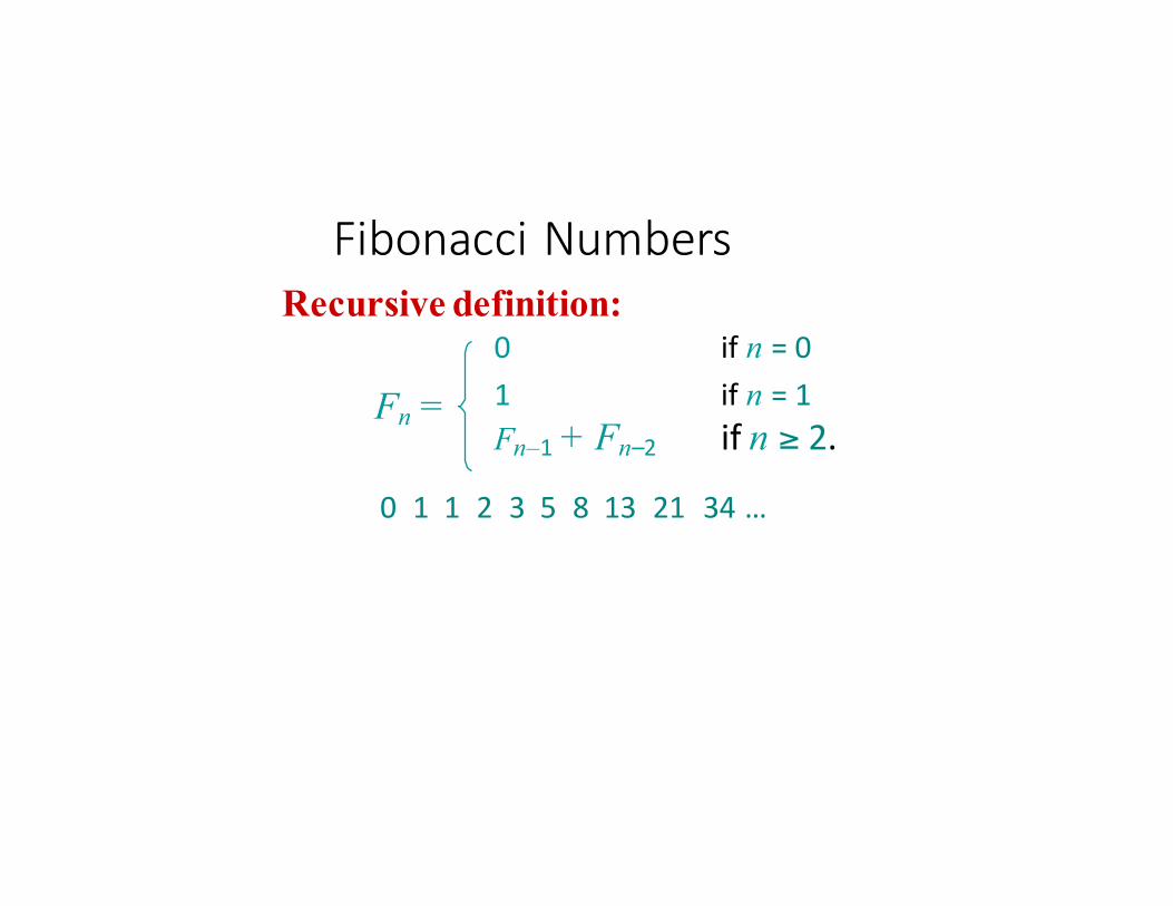
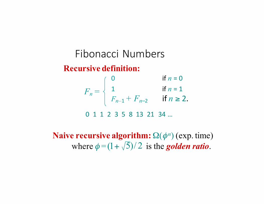
Fibonacci NumbersRecursive definition:
Fn =0 if n = 01 if n = 1Fn–1+ Fn–2 if n ≥ 2.
0 1 1 2 3 5 8 13 21 34 …
Fibonacci NumbersRecursive definition:
Fn =0 if n = 01 if n = 1Fn–1+ Fn–2 if n ≥ 2.
0 1 1 2 3 5 8 13 21 34 …
5)/ 2Naive recursive algorithm:Ω(φ n) (exp. time)
where φ =(1+ is the golden ratio.
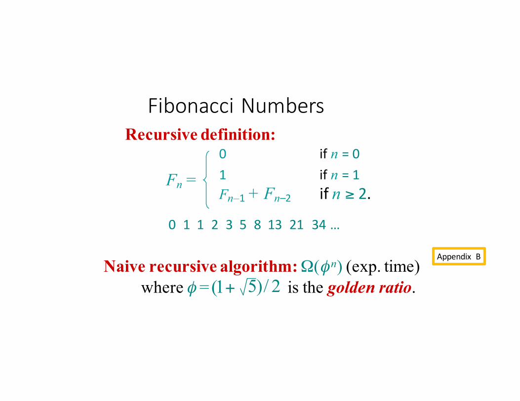
Fibonacci NumbersRecursive definition:
Fn =0 if n = 01 if n = 1Fn–1+ Fn–2 if n ≥ 2.
0 1 1 2 3 5 8 13 21 34 …
5)/ 2Naive recursive algorithm:Ω(φ n) (exp. time)
where φ =(1+ is the golden ratio.
Appendix B
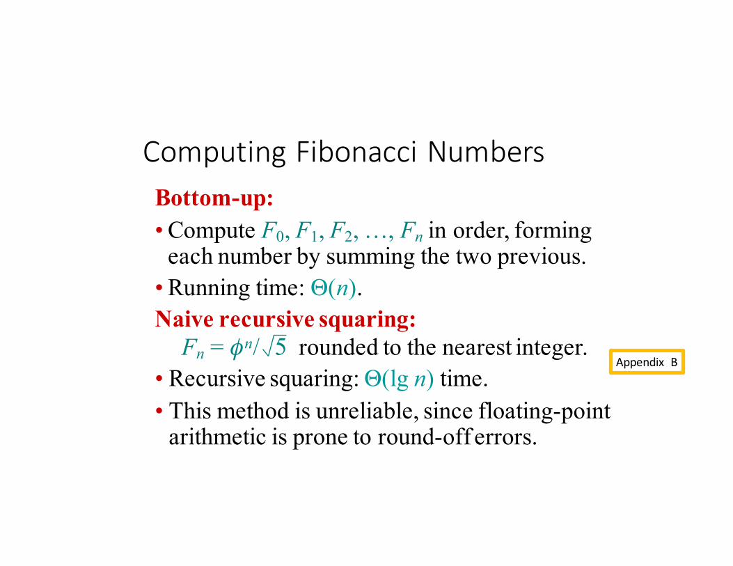
Computing FibonacciNumbersBottom-up:• Compute F0, F1, F2, …, Fn in order, forming
each number by summing the two previous.• Running time: Θ(n).Naive recursive squaring:
Fn = φ n/ 5 rounded to the nearest integer.• Recursive squaring:Θ(lg n) time.• This method is unreliable, since floating-point
arithmetic is prone to round-off errors.
Appendix B
MatrixMultiplication
9/28/16, 9:42 PMStrassen algorithm - Wikipedia, the free encyclopedia
Page 2 of 6https://en.wikipedia.org/wiki/Strassen_algorithm
The left column represents 2x2 matrix multiplication. Naïve matrix multiplication requires one multiplication for each "1" of the left column.Each of the other columns represents a single one of the 7 multiplications in the algorithm, and the sum of the columns gives the full matrixmultiplication on the left.
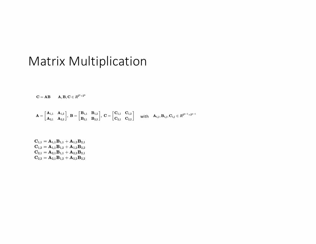
Let A, B be two square matrices over a ring R. We want to calculate the matrix product C as
If the matrices A, B are not of type 2n × 2n we fill the missing rows and columns with zeros.
We partition A, B and C into equally sized block matrices
with
then
With this construction we have not reduced the number of multiplications. We still need 8 multiplications to calculate the Ci,jmatrices, the same number of multiplications we need when using standard matrix multiplication.
Now comes the important part. We define new matrices
9/28/16, 9:42 PMStrassen algorithm - Wikipedia, the free encyclopedia
Page 2 of 6https://en.wikipedia.org/wiki/Strassen_algorithm
The left column represents 2x2 matrix multiplication. Naïve matrix multiplication requires one multiplication for each "1" of the left column.Each of the other columns represents a single one of the 7 multiplications in the algorithm, and the sum of the columns gives the full matrixmultiplication on the left.
Let A, B be two square matrices over a ring R. We want to calculate the matrix product C as
If the matrices A, B are not of type 2n × 2n we fill the missing rows and columns with zeros.
We partition A, B and C into equally sized block matrices
with
then
With this construction we have not reduced the number of multiplications. We still need 8 multiplications to calculate the Ci,jmatrices, the same number of multiplications we need when using standard matrix multiplication.
Now comes the important part. We define new matrices
with
9/28/16, 9:42 PMStrassen algorithm - Wikipedia, the free encyclopedia
Page 2 of 6https://en.wikipedia.org/wiki/Strassen_algorithm
The left column represents 2x2 matrix multiplication. Naïve matrix multiplication requires one multiplication for each "1" of the left column.Each of the other columns represents a single one of the 7 multiplications in the algorithm, and the sum of the columns gives the full matrixmultiplication on the left.
Let A, B be two square matrices over a ring R. We want to calculate the matrix product C as
If the matrices A, B are not of type 2n × 2n we fill the missing rows and columns with zeros.
We partition A, B and C into equally sized block matrices
with
then
With this construction we have not reduced the number of multiplications. We still need 8 multiplications to calculate the Ci,jmatrices, the same number of multiplications we need when using standard matrix multiplication.
Now comes the important part. We define new matrices
MatrixMultiplication4.2 Strassen’s algorithm for matrix multiplication 77
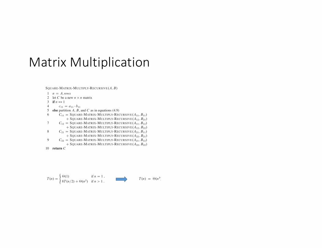
SQUARE-MATRIX-MULTIPLY-RECURSIVE.A; B/
1 n D A:rows2 let C be a new n ! n matrix3 if n == 14 c11 D a11 " b11
5 else partition A, B , and C as in equations (4.9)6 C11 D SQUARE-MATRIX-MULTIPLY-RECURSIVE.A11; B11/
C SQUARE-MATRIX-MULTIPLY-RECURSIVE.A12; B21/7 C12 D SQUARE-MATRIX-MULTIPLY-RECURSIVE.A11; B12/
C SQUARE-MATRIX-MULTIPLY-RECURSIVE.A12; B22/8 C21 D SQUARE-MATRIX-MULTIPLY-RECURSIVE.A21; B11/
C SQUARE-MATRIX-MULTIPLY-RECURSIVE.A22; B21/9 C22 D SQUARE-MATRIX-MULTIPLY-RECURSIVE.A21; B12/
C SQUARE-MATRIX-MULTIPLY-RECURSIVE.A22; B22/10 return C
This pseudocode glosses over one subtle but important implementation detail.How do we partition the matrices in line 5? If we were to create 12 new n=2 ! n=2matrices, we would spend ‚.n2/ time copying entries. In fact, we can partitionthe matrices without copying entries. The trick is to use index calculations. Weidentify a submatrix by a range of row indices and a range of column indices ofthe original matrix. We end up representing a submatrix a little differently fromhow we represent the original matrix, which is the subtlety we are glossing over.The advantage is that, since we can specify submatrices by index calculations,executing line 5 takes only ‚.1/ time (although we shall see that it makes nodifference asymptotically to the overall running time whether we copy or partitionin place).
Now, we derive a recurrence to characterize the running time of SQUARE-MATRIX-MULTIPLY-RECURSIVE. Let T .n/ be the time to multiply two n ! nmatrices using this procedure. In the base case, when n D 1, we perform just theone scalar multiplication in line 4, and soT .1/ D ‚.1/ : (4.15)
The recursive case occurs when n > 1. As discussed, partitioning the matrices inline 5 takes ‚.1/ time, using index calculations. In lines 6–9, we recursively callSQUARE-MATRIX-MULTIPLY-RECURSIVE a total of eight times. Because eachrecursive call multiplies two n=2 ! n=2 matrices, thereby contributing T .n=2/ tothe overall running time, the time taken by all eight recursive calls is 8T .n=2/. Wealso must account for the four matrix additions in lines 6–9. Each of these matricescontains n2=4 entries, and so each of the four matrix additions takes ‚.n2/ time.Since the number of matrix additions is a constant, the total time spent adding ma-
78 Chapter 4 Divide-and-Conquer
trices in lines 6–9 is ‚.n2/. (Again, we use index calculations to place the resultsof the matrix additions into the correct positions of matrix C , with an overheadof ‚.1/ time per entry.) The total time for the recursive case, therefore, is the sumof the partitioning time, the time for all the recursive calls, and the time to add thematrices resulting from the recursive calls:T .n/ D ‚.1/C 8T .n=2/C‚.n2/
D 8T .n=2/C‚.n2/ : (4.16)Notice that if we implemented partitioning by copying matrices, which would cost‚.n2/ time, the recurrence would not change, and hence the overall running timewould increase by only a constant factor.
Combining equations (4.15) and (4.16) gives us the recurrence for the runningtime of SQUARE-MATRIX-MULTIPLY-RECURSIVE:
T .n/ D
(‚.1/ if n D 1 ;
8T .n=2/C‚.n2/ if n > 1 :(4.17)
As we shall see from the master method in Section 4.5, recurrence (4.17) has thesolution T .n/ D ‚.n3/. Thus, this simple divide-and-conquer approach is nofaster than the straightforward SQUARE-MATRIX-MULTIPLY procedure.
Before we continue on to examining Strassen’s algorithm, let us review wherethe components of equation (4.16) came from. Partitioning each n ! n matrix byindex calculation takes ‚.1/ time, but we have two matrices to partition. Althoughyou could say that partitioning the two matrices takes ‚.2/ time, the constant of 2is subsumed by the ‚-notation. Adding two matrices, each with, say, k entries,takes ‚.k/ time. Since the matrices we add each have n2=4 entries, you couldsay that adding each pair takes ‚.n2=4/ time. Again, however, the ‚-notationsubsumes the constant factor of 1=4, and we say that adding two n2=4 ! n2=4matrices takes ‚.n2/ time. We have four such matrix additions, and once again,instead of saying that they take ‚.4n2/ time, we say that they take ‚.n2/ time.(Of course, you might observe that we could say that the four matrix additionstake ‚.4n2=4/ time, and that 4n2=4 D n2, but the point here is that ‚-notationsubsumes constant factors, whatever they are.) Thus, we end up with two termsof ‚.n2/, which we can combine into one.
When we account for the eight recursive calls, however, we cannot just sub-sume the constant factor of 8. In other words, we must say that together they take8T .n=2/ time, rather than just T .n=2/ time. You can get a feel for why by lookingback at the recursion tree in Figure 2.5, for recurrence (2.1) (which is identical torecurrence (4.7)), with the recursive case T .n/ D 2T .n=2/C‚.n/. The factor of 2determined how many children each tree node had, which in turn determined howmany terms contributed to the sum at each level of the tree. If we were to ignore
Strassen algorithm
9/28/16, 9:42 PMStrassen algorithm - Wikipedia, the free encyclopedia
Page 2 of 6https://en.wikipedia.org/wiki/Strassen_algorithm
The left column represents 2x2 matrix multiplication. Naïve matrix multiplication requires one multiplication for each "1" of the left column.Each of the other columns represents a single one of the 7 multiplications in the algorithm, and the sum of the columns gives the full matrixmultiplication on the left.
Let A, B be two square matrices over a ring R. We want to calculate the matrix product C as
If the matrices A, B are not of type 2n × 2n we fill the missing rows and columns with zeros.
We partition A, B and C into equally sized block matrices
with
then
With this construction we have not reduced the number of multiplications. We still need 8 multiplications to calculate the Ci,jmatrices, the same number of multiplications we need when using standard matrix multiplication.
Now comes the important part. We define new matrices
9/28/16, 9:42 PMStrassen algorithm - Wikipedia, the free encyclopedia
Page 3 of 6https://en.wikipedia.org/wiki/Strassen_algorithm
only using 7 multiplications (one for each Mk) instead of 8. We may now express the Ci,j in terms of Mk, like this:
We iterate this division process n times (recursively) until the submatrices degenerate into numbers (elements of the ring R).The resulting product will be padded with zeroes just like A and B, and should be stripped of the corresponding rows andcolumns.
Practical implementations of Strassen's algorithm switch to standard methods of matrix multiplication for small enoughsubmatrices, for which those algorithms are more efficient. The particular crossover point for which Strassen's algorithm ismore efficient depends on the specific implementation and hardware. Earlier authors had estimated that Strassen's algorithm isfaster for matrices with widths from 32 to 128 for optimized implementations.[1] However, it has been observed that thiscrossover point has been increasing in recent years, and a 2010 study found that even a single step of Strassen's algorithm isoften not beneficial on current architectures, compared to a highly optimized traditional multiplication, until matrix sizesexceed 1000 or more, and even for matrix sizes of several thousand the benefit is typically marginal at best (around 10% orless).[2]
Asymptotic complexity
The standard matrix multiplication takes approximately 2N3 (where N = 2n) arithmetic operations (additions andmultiplications); the asymptotic complexity is Θ(N3).
The number of additions and multiplications required in the Strassen algorithm can be calculated as follows: let f(n) be thenumber of operations for a 2n × 2n matrix. Then by recursive application of the Strassen algorithm, we see thatf(n) = 7f(n−1) + ℓ4n, for some constant ℓ that depends on the number of additions performed at each application of thealgorithm. Hence f(n) = (7 + o(1))n, i.e., the asymptotic complexity for multiplying matrices of size N = 2n using theStrassen algorithm is
.
The reduction in the number of arithmetic operations however comes at the price of a somewhat reduced numericalstability,[3] and the algorithm also requires significantly more memory compared to the naive algorithm. Both initial matricesmust have their dimensions expanded to the next power of 2, which results in storing up to four times as many elements, andthe seven auxiliary matrices each contain a quarter of the elements in the expanded ones.
Rank or bilinear complexity
The bilinear complexity or rank of a bilinear map is an important concept in the asymptotic complexity of matrixmultiplication. The rank of a bilinear map over a field F is defined as (somewhat of an abuse of notation)
4.2 Strassen’s algorithm for matrix multiplication 79
the factor of 8 in equation (4.16) or the factor of 2 in recurrence (4.1), the recursiontree would just be linear, rather than “bushy,” and each level would contribute onlyone term to the sum.
Bear in mind, therefore, that although asymptotic notation subsumes constantmultiplicative factors, recursive notation such as T .n=2/ does not.
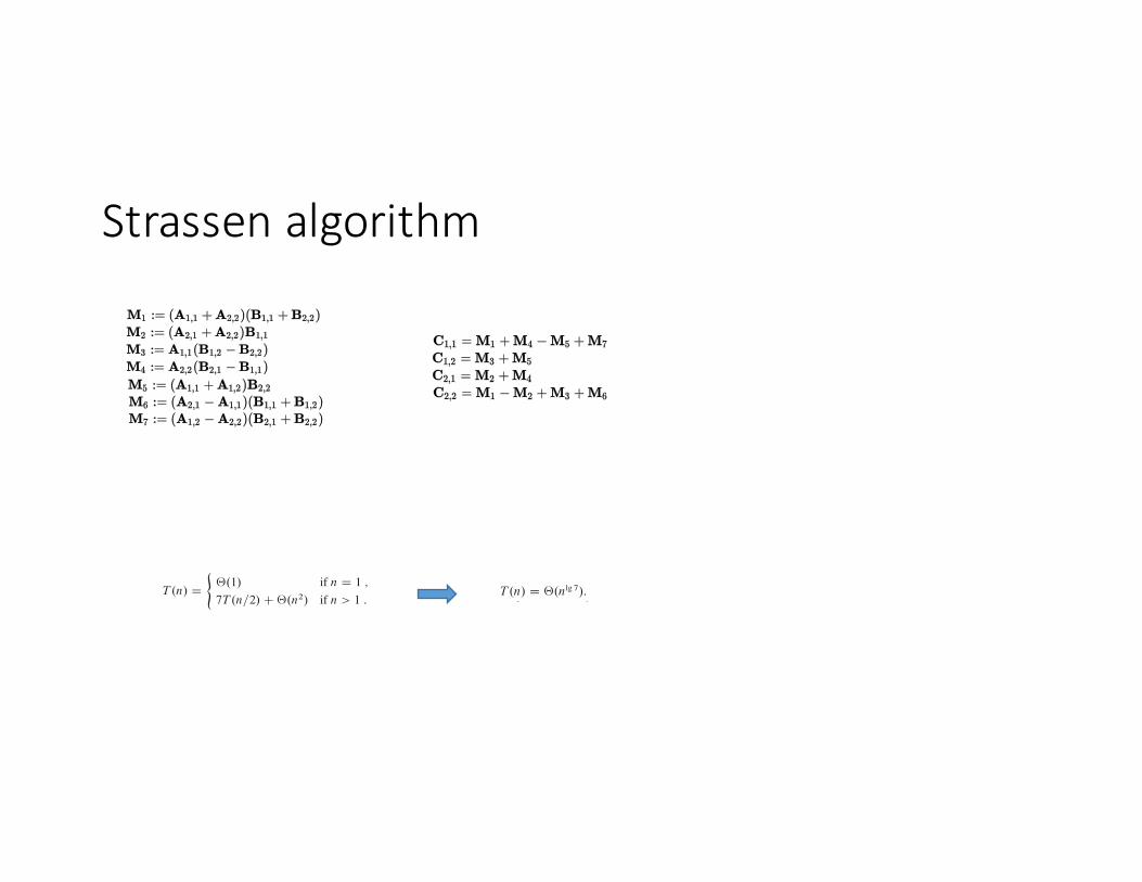
Strassen’s methodThe key to Strassen’s method is to make the recursion tree slightly less bushy. Thatis, instead of performing eight recursive multiplications of n=2 ! n=2 matrices,it performs only seven. The cost of eliminating one matrix multiplication will beseveral new additions of n=2 ! n=2 matrices, but still only a constant number ofadditions. As before, the constant number of matrix additions will be subsumedby ‚-notation when we set up the recurrence equation to characterize the runningtime.
Strassen’s method is not at all obvious. (This might be the biggest understate-ment in this book.) It has four steps:1. Divide the input matrices A and B and output matrix C into n=2 ! n=2 subma-
trices, as in equation (4.9). This step takes ‚.1/ time by index calculation, justas in SQUARE-MATRIX-MULTIPLY-RECURSIVE.
2. Create 10 matrices S1; S2; : : : ; S10, each of which is n=2 ! n=2 and is the sumor difference of two matrices created in step 1. We can create all 10 matrices in‚.n2/ time.
3. Using the submatrices created in step 1 and the 10 matrices created in step 2,recursively compute seven matrix products P1; P2; : : : ; P7. Each matrix Pi isn=2 ! n=2.
4. Compute the desired submatrices C11; C12; C21; C22 of the result matrix C byadding and subtracting various combinations of the Pi matrices. We can com-pute all four submatrices in ‚.n2/ time.
We shall see the details of steps 2–4 in a moment, but we already have enoughinformation to set up a recurrence for the running time of Strassen’s method. Let usassume that once the matrix size n gets down to 1, we perform a simple scalar mul-tiplication, just as in line 4 of SQUARE-MATRIX-MULTIPLY-RECURSIVE. Whenn > 1, steps 1, 2, and 4 take a total of ‚.n2/ time, and step 3 requires us to per-form seven multiplications of n=2 ! n=2 matrices. Hence, we obtain the followingrecurrence for the running time T .n/ of Strassen’s algorithm:
T .n/ D
(‚.1/ if n D 1 ;
7T .n=2/C‚.n2/ if n > 1 :(4.18)
80 Chapter 4 Divide-and-Conquer
We have traded off one matrix multiplication for a constant number of matrix ad-ditions. Once we understand recurrences and their solutions, we shall see that thistradeoff actually leads to a lower asymptotic running time. By the master methodin Section 4.5, recurrence (4.18) has the solution T .n/ D ‚.nlg 7/.
We now proceed to describe the details. In step 2, we create the following 10matrices:S1 D B12 ! B22 ;
S2 D A11 C A12 ;
S3 D A21 C A22 ;
S4 D B21 ! B11 ;
S5 D A11 C A22 ;
S6 D B11 C B22 ;
S7 D A12 ! A22 ;
S8 D B21 C B22 ;
S9 D A11 ! A21 ;
S10 D B11 C B12 :
Since we must add or subtract n=2 " n=2 matrices 10 times, this step does indeedtake ‚.n2/ time.
In step 3, we recursively multiply n=2"n=2 matrices seven times to compute thefollowing n=2 " n=2 matrices, each of which is the sum or difference of productsof A and B submatrices:P1 D A11 # S1 D A11 # B12 ! A11 # B22 ;
P2 D S2 # B22 D A11 # B22 C A12 # B22 ;
P3 D S3 # B11 D A21 # B11 C A22 # B11 ;
P4 D A22 # S4 D A22 # B21 ! A22 # B11 ;
P5 D S5 # S6 D A11 # B11 C A11 # B22 C A22 # B11 C A22 # B22 ;
P6 D S7 # S8 D A12 # B21 C A12 # B22 ! A22 # B21 ! A22 # B22 ;
P7 D S9 # S10 D A11 # B11 C A11 # B12 ! A21 # B11 ! A21 # B12 :
Note that the only multiplications we need to perform are those in the middle col-umn of the above equations. The right-hand column just shows what these productsequal in terms of the original submatrices created in step 1.
Step 4 adds and subtracts the Pi matrices created in step 3 to construct the fourn=2 " n=2 submatrices of the product C . We start withC11 D P5 C P4 ! P2 C P6 :