Distance metrics for Sequential Data
73
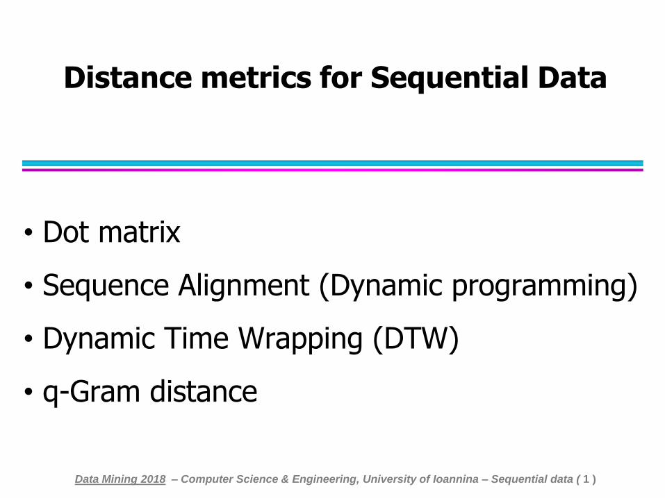
Distance metrics for Sequential Data • Dot matrix • Sequence Alignment (Dynamic programming) • Dynamic Time Wrapping (DTW) • q-Gram distance Data Mining 2018 – Computer Science & Engineering, University of Ioannina – Sequential data ( 1 )
Transcript of Distance metrics for Sequential Data
Distance metrics for Sequential Data
• Dot matrix
• Sequence Alignment (Dynamic programming)
• Dynamic Time Wrapping (DTW)
• q-Gram distance
Data Mining 2018 – Computer Science & Engineering, University of Ioannina – Sequential data ( 1 )
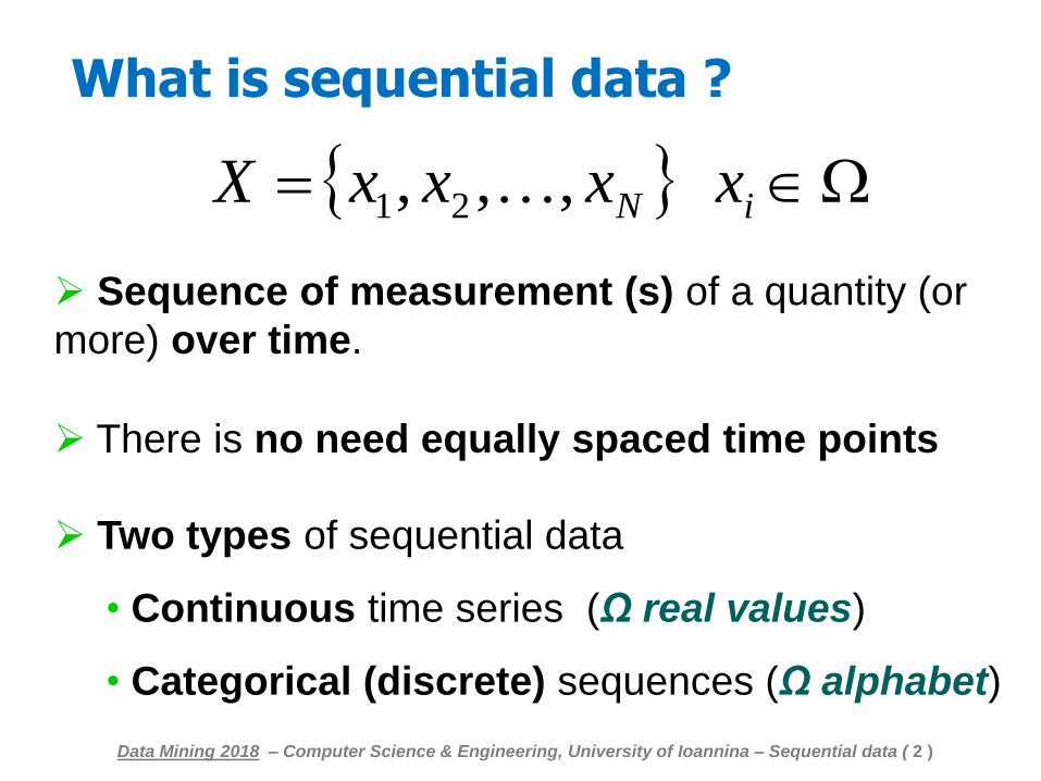
Sequence of measurement (s) of a quantity (or
more) over time.
There is no need equally spaced time points
Two types of sequential data
• Continuous time series (Ω real values)
• Categorical (discrete) sequences (Ω alphabet)
What is sequential data ?
Data Mining 2018 – Computer Science & Engineering, University of Ioannina – Sequential data ( 2 )
NxxxX ,,, 21 ix
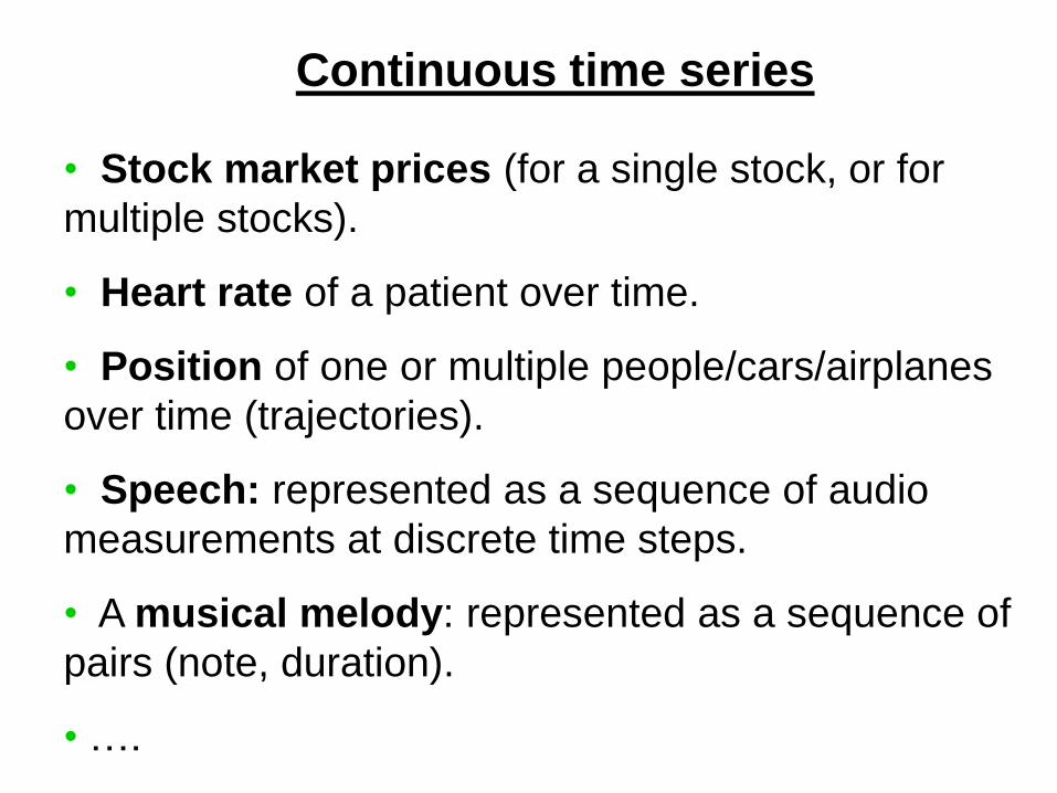
Continuous time series
• Stock market prices (for a single stock, or for
multiple stocks).
• Heart rate of a patient over time.
• Position of one or multiple people/cars/airplanes
over time (trajectories).
• Speech: represented as a sequence of audio
measurements at discrete time steps.
• A musical melody: represented as a sequence of
pairs (note, duration).
• ….
Categorical (discrete) sequences
• Biological sequences (DNA / Protein)
• Web navigation
• Song listening sequences
• Sunny/Rainy weather sequences
• Mobility in a network of cities / regions
• ...
Data Mining 2018 – Computer Science & Engineering, University of Ioannina – Sequential data ( 4 )
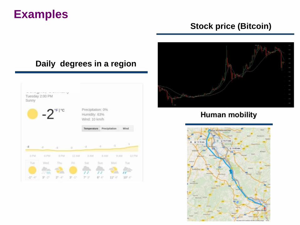
Examples Stock price (Bitcoin)
Daily degrees in a region
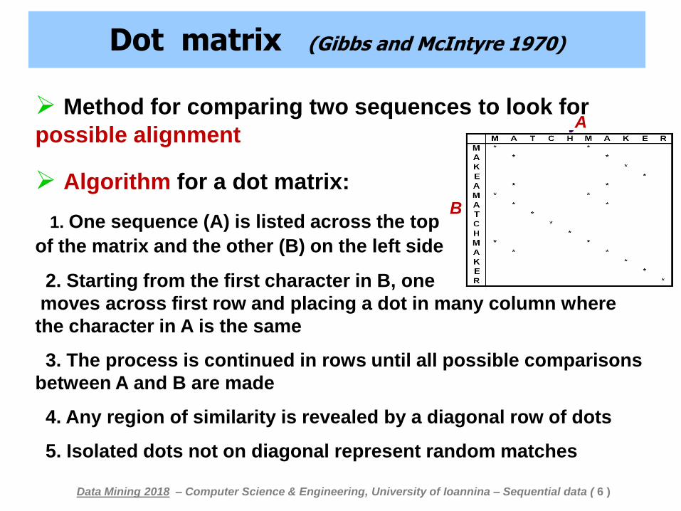
Method for comparing two sequences to look for
possible alignment
Algorithm for a dot matrix:
1. One sequence (A) is listed across the top
of the matrix and the other (B) on the left side
2. Starting from the first character in B, one
moves across first row and placing a dot in many column where
the character in A is the same
3. The process is continued in rows until all possible comparisons
between A and B are made
4. Any region of similarity is revealed by a diagonal row of dots
5. Isolated dots not on diagonal represent random matches
Dot matrix (Gibbs and McIntyre 1970)
A
B
Data Mining 2018 – Computer Science & Engineering, University of Ioannina – Sequential data ( 6 )
Dot matrix
Improve visualization of identical regions
among sequences by using sliding
windows, instead of writing down a dot for
every character, that is common in both
sequences
We compare a number of positions
(window size), and we write down a dot
whenever there is minimum number of
identical characters
Data Mining 2018 – Computer Science & Engineering, University of Ioannina – Sequential data ( 7 )
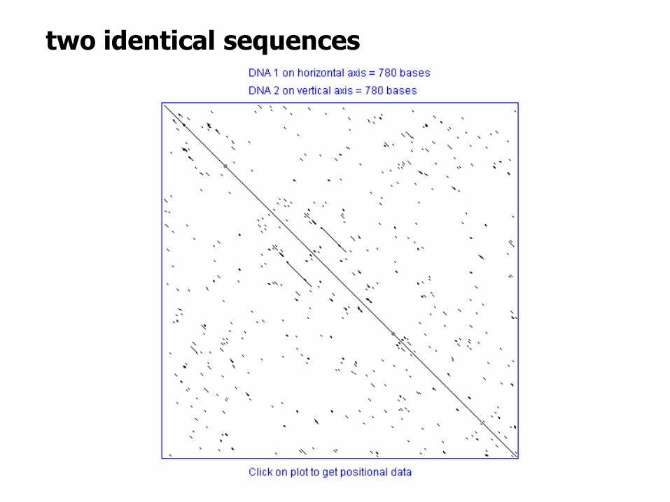
two identical sequences
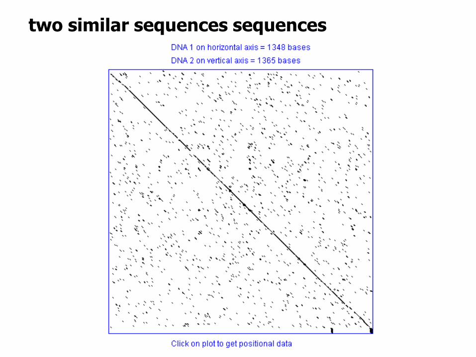
two similar sequences sequences
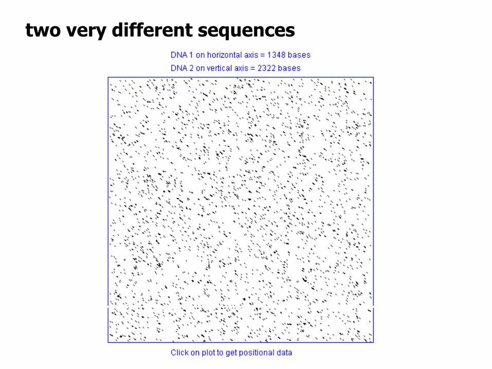
two very different sequences
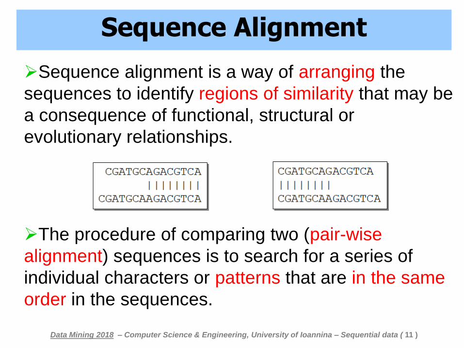
Sequence alignment is a way of arranging the
sequences to identify regions of similarity that may be
a consequence of functional, structural or
evolutionary relationships.
The procedure of comparing two (pair-wise
alignment) sequences is to search for a series of
individual characters or patterns that are in the same
order in the sequences.
Sequence Alignment
Data Mining 2018 – Computer Science & Engineering, University of Ioannina – Sequential data ( 11 )
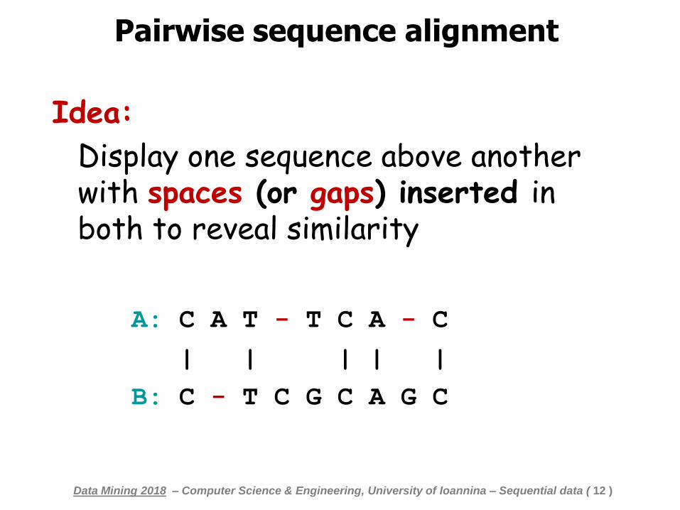
Pairwise sequence alignment
A: C A T - T C A - C
| | | | |
B: C - T C G C A G C
Idea:
Display one sequence above another with spaces (or gaps) inserted in both to reveal similarity
Data Mining 2018 – Computer Science & Engineering, University of Ioannina – Sequential data ( 12 )
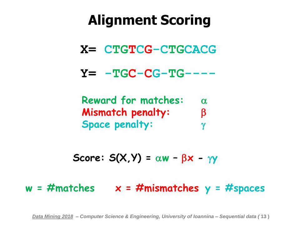
X= CTGTCG-CTGCACG
Y= -TGC-CG-TG----
Reward for matches: Mismatch penalty: Space penalty:
Score: S(X,Y) = w – x - y
w = #matches x = #mismatches y = #spaces
Alignment Scoring
Data Mining 2018 – Computer Science & Engineering, University of Ioannina – Sequential data ( 13 )
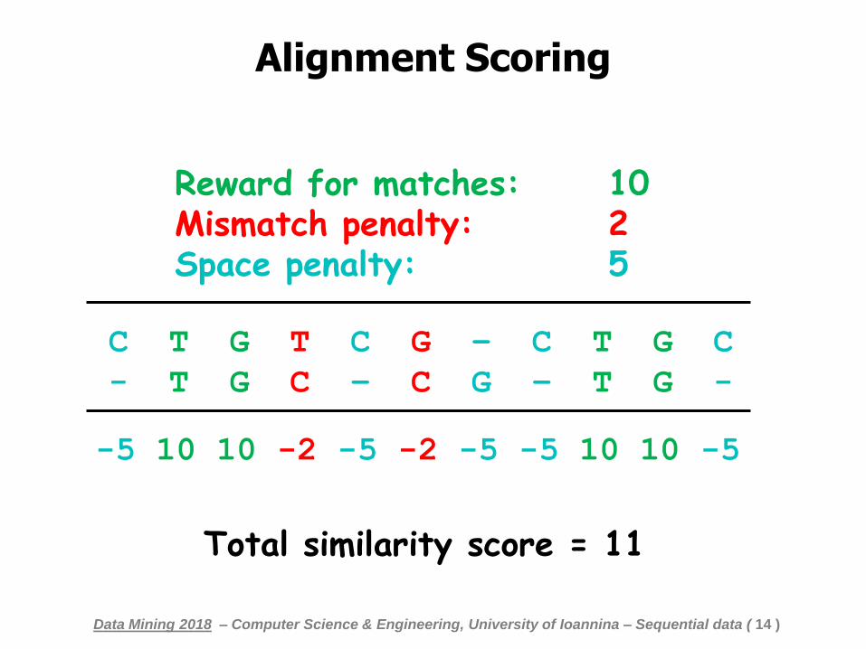
Alignment Scoring
C T G T C G – C T G C
- T G C – C G – T G -
-5 10 10 -2 -5 -2 -5 -5 10 10 -5
Total similarity score = 11
Reward for matches: 10 Mismatch penalty: 2 Space penalty: 5
Data Mining 2018 – Computer Science & Engineering, University of Ioannina – Sequential data ( 14 )
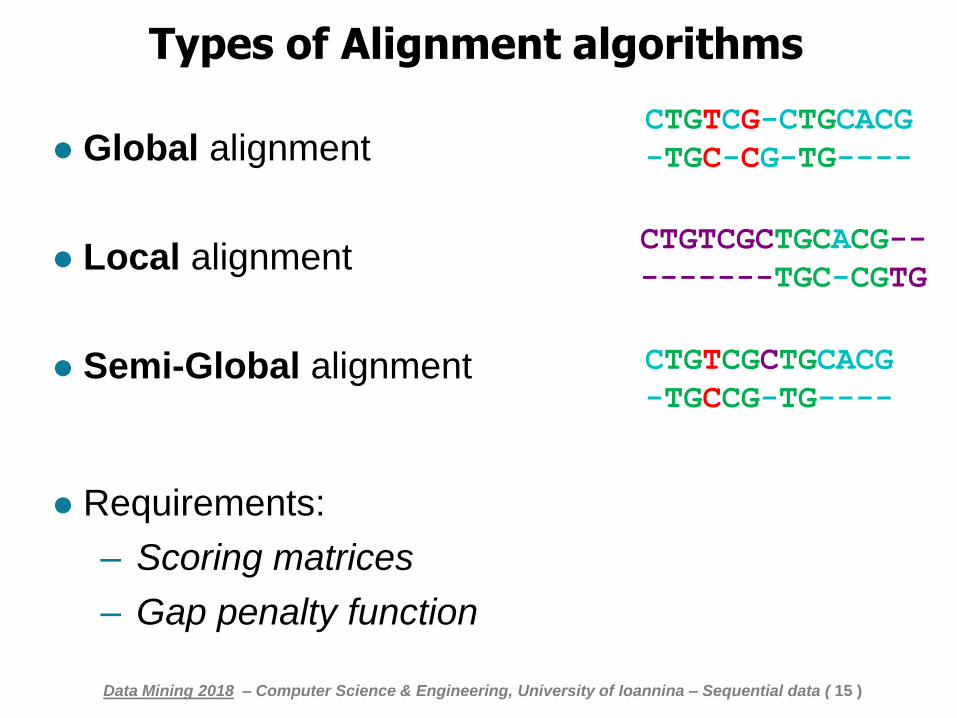
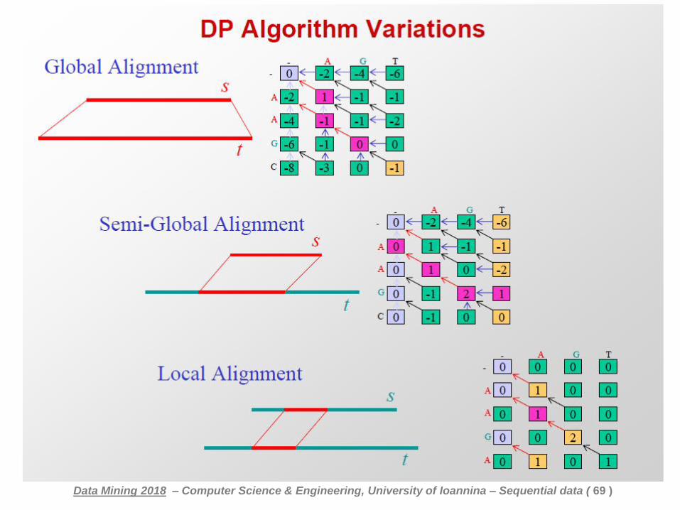
Types of Alignment algorithms
Global alignment
Local alignment
Semi-Global alignment
Requirements:
– Scoring matrices
– Gap penalty function
CTGTCG-CTGCACG
-TGC-CG-TG----
CTGTCGCTGCACG--
-------TGC-CGTG
CTGTCGCTGCACG
-TGCCG-TG----
Data Mining 2018 – Computer Science & Engineering, University of Ioannina – Sequential data ( 15 )
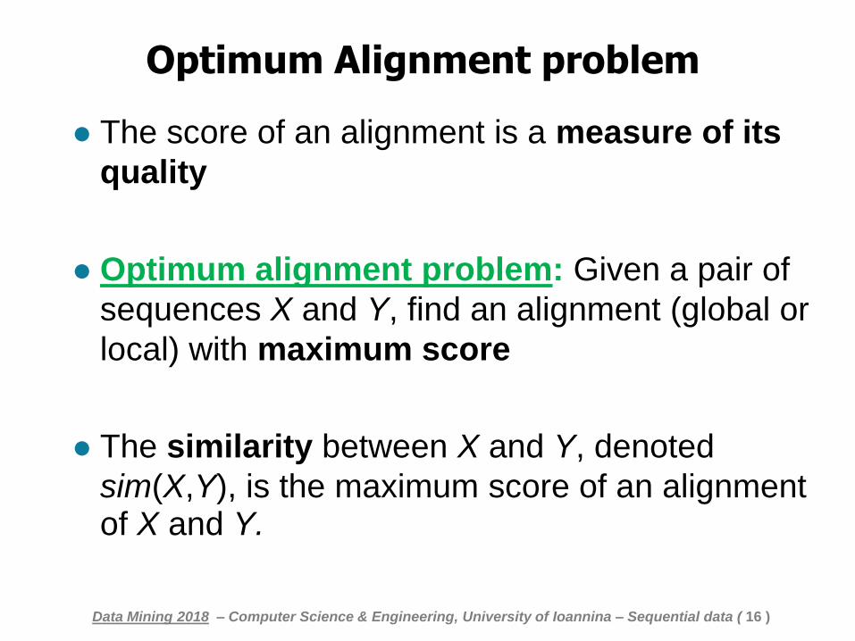
Optimum Alignment problem
The score of an alignment is a measure of its
quality
Optimum alignment problem: Given a pair of
sequences X and Y, find an alignment (global or
local) with maximum score
The similarity between X and Y, denoted
sim(X,Y), is the maximum score of an alignment of X and Y.
Data Mining 2018 – Computer Science & Engineering, University of Ioannina – Sequential data ( 16 )
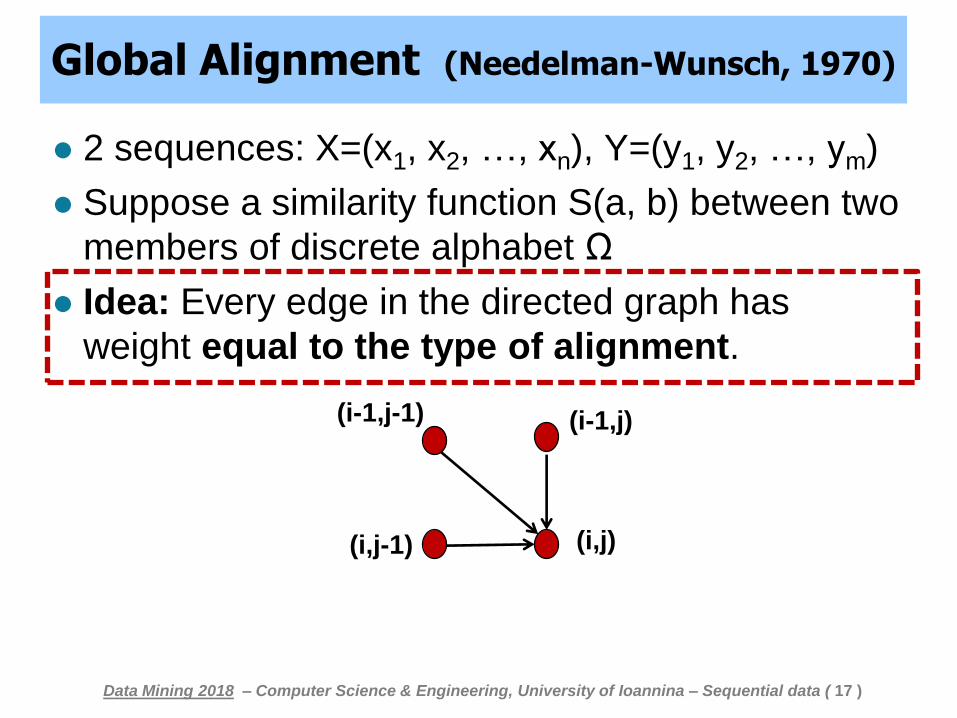
Global Alignment (Needelman-Wunsch, 1970)
2 sequences: X=(x1, x2, …, xn), Y=(y1, y2, …, ym)
Suppose a similarity function S(a, b) between two
members of discrete alphabet Ω
Idea: Every edge in the directed graph has
weight equal to the type of alignment.
(i-1,j-1)
(i,j)
(i-1,j)
(i,j-1)
Data Mining 2018 – Computer Science & Engineering, University of Ioannina – Sequential data ( 17 )
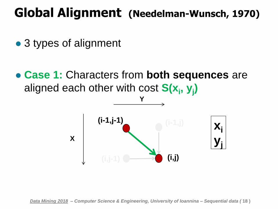
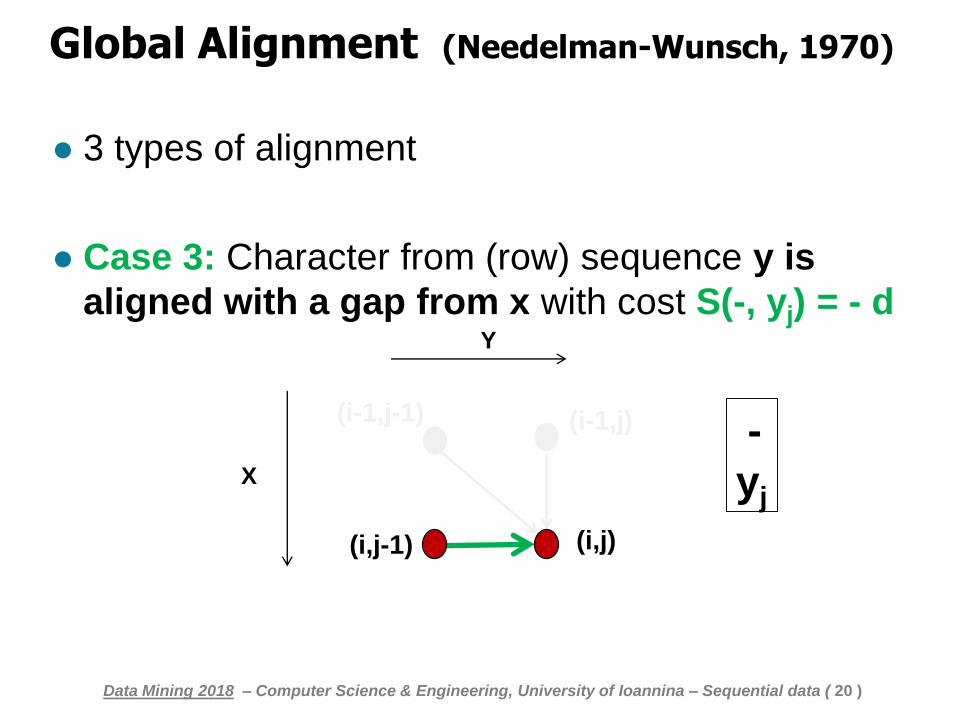
Global Alignment (Needelman-Wunsch, 1970)
3 types of alignment
Case 1: Characters from both sequences are
aligned each other with cost S(xi, yj)
(i-1,j-1)
(i,j)
(i-1,j)
(i,j-1)
xi
yj
Y
X
Data Mining 2018 – Computer Science & Engineering, University of Ioannina – Sequential data ( 18 )
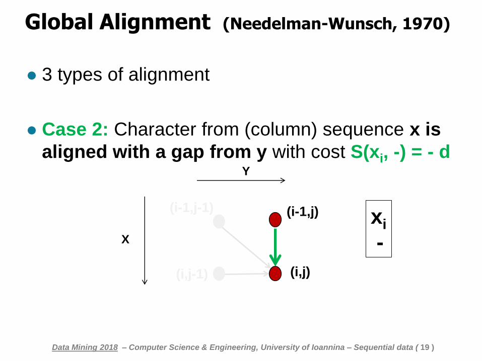
Global Alignment (Needelman-Wunsch, 1970)
3 types of alignment
Case 2: Character from (column) sequence x is
aligned with a gap from y with cost S(xi, -) = - d
(i-1,j-1)
(i,j)
(i-1,j)
(i,j-1)
xi
-
Y
X
Data Mining 2018 – Computer Science & Engineering, University of Ioannina – Sequential data ( 19 )
Global Alignment (Needelman-Wunsch, 1970)
3 types of alignment
Case 3: Character from (row) sequence y is
aligned with a gap from x with cost S(-, yj) = - d
(i-1,j-1)
(i,j)
(i-1,j)
(i,j-1)
-
yj
Y
X
Data Mining 2018 – Computer Science & Engineering, University of Ioannina – Sequential data ( 20 )
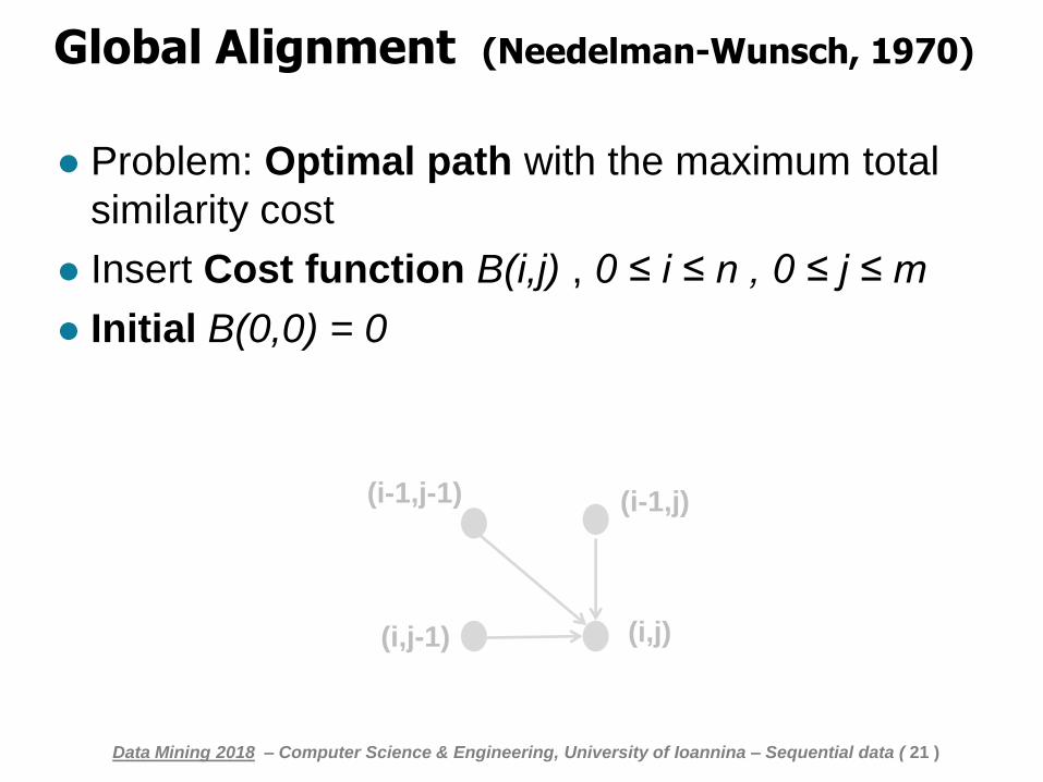
Global Alignment (Needelman-Wunsch, 1970)
Problem: Optimal path with the maximum total
similarity cost
Insert Cost function B(i,j) , 0 ≤ i ≤ n , 0 ≤ j ≤ m
Initial B(0,0) = 0
(i-1,j-1)
(i,j)
(i-1,j)
(i,j-1)
Data Mining 2018 – Computer Science & Engineering, University of Ioannina – Sequential data ( 21 )
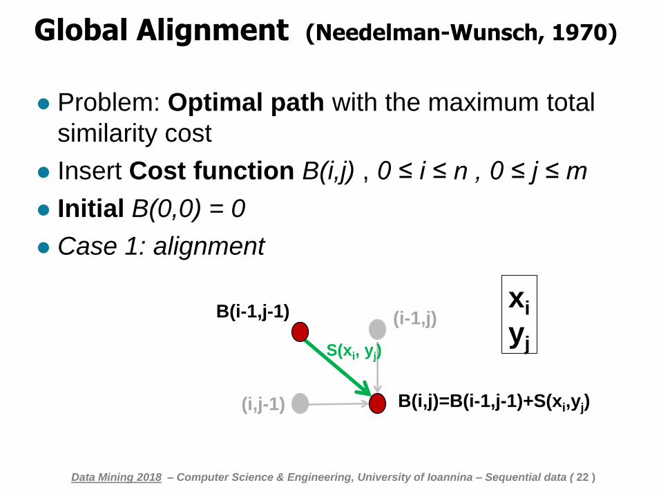
Global Alignment (Needelman-Wunsch, 1970)
Problem: Optimal path with the maximum total
similarity cost
Insert Cost function B(i,j) , 0 ≤ i ≤ n , 0 ≤ j ≤ m
Initial B(0,0) = 0
Case 1: alignment
B(i-1,j-1)
B(i,j)=B(i-1,j-1)+S(xi,yj)
(i-1,j)
(i,j-1)
S(xi, yj)
xi
yj
Data Mining 2018 – Computer Science & Engineering, University of Ioannina – Sequential data ( 22 )
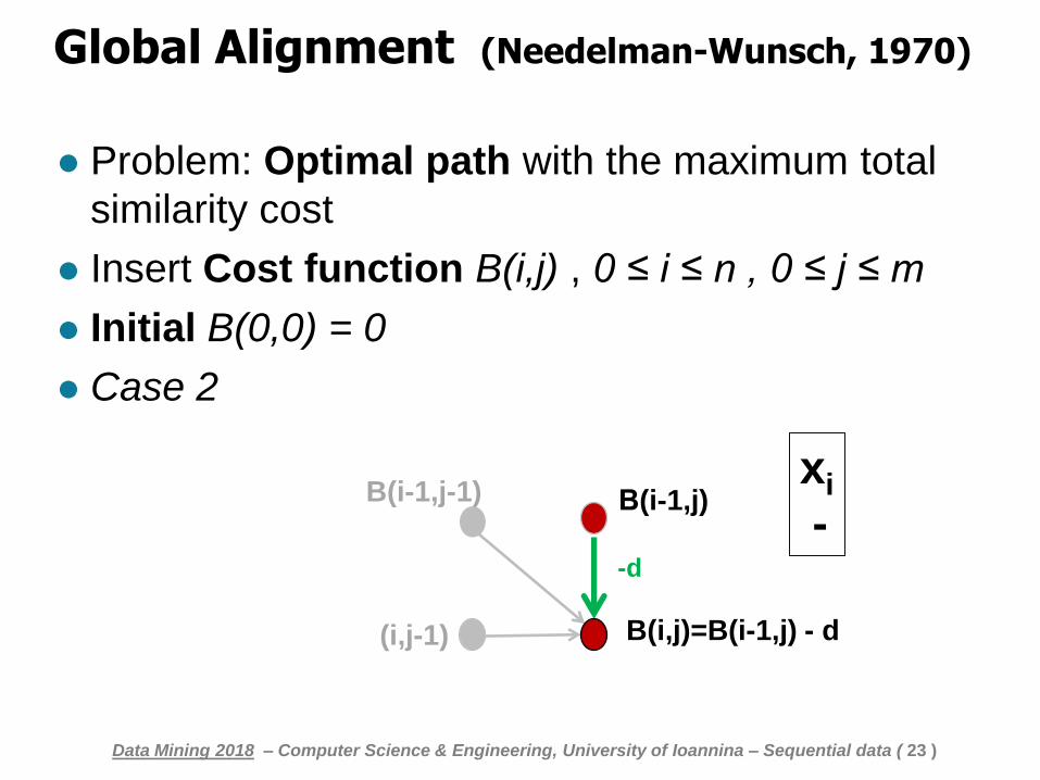
Global Alignment (Needelman-Wunsch, 1970)
Problem: Optimal path with the maximum total
similarity cost
Insert Cost function B(i,j) , 0 ≤ i ≤ n , 0 ≤ j ≤ m
Initial B(0,0) = 0
Case 2
B(i-1,j-1)
B(i,j)=B(i-1,j) - d
Β(i-1,j)
(i,j-1)
-d
xi
-
Data Mining 2018 – Computer Science & Engineering, University of Ioannina – Sequential data ( 23 )
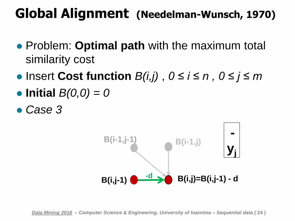
Global Alignment (Needelman-Wunsch, 1970)
Problem: Optimal path with the maximum total
similarity cost
Insert Cost function B(i,j) , 0 ≤ i ≤ n , 0 ≤ j ≤ m
Initial B(0,0) = 0
Case 3
B(i-1,j-1)
B(i,j)=B(i,j-1) - d
Β(i-1,j)
B(i,j-1) -d
-
yj
Data Mining 2018 – Computer Science & Engineering, University of Ioannina – Sequential data ( 24 )
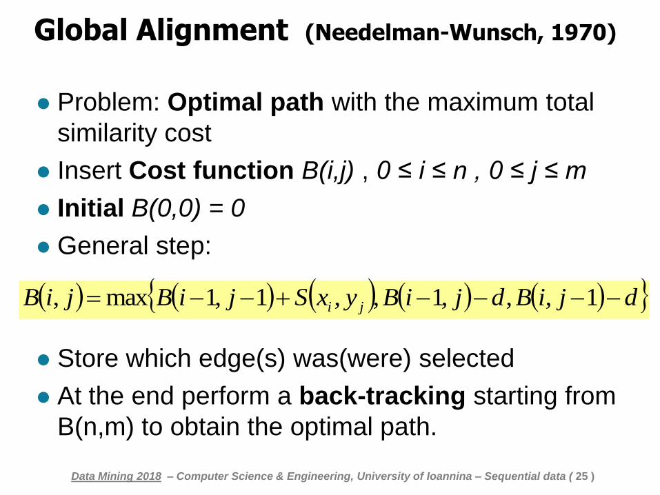
Global Alignment (Needelman-Wunsch, 1970)
Problem: Optimal path with the maximum total
similarity cost
Insert Cost function B(i,j) , 0 ≤ i ≤ n , 0 ≤ j ≤ m
Initial B(0,0) = 0
General step:
Store which edge(s) was(were) selected
At the end perform a back-tracking starting from
B(n,m) to obtain the optimal path.
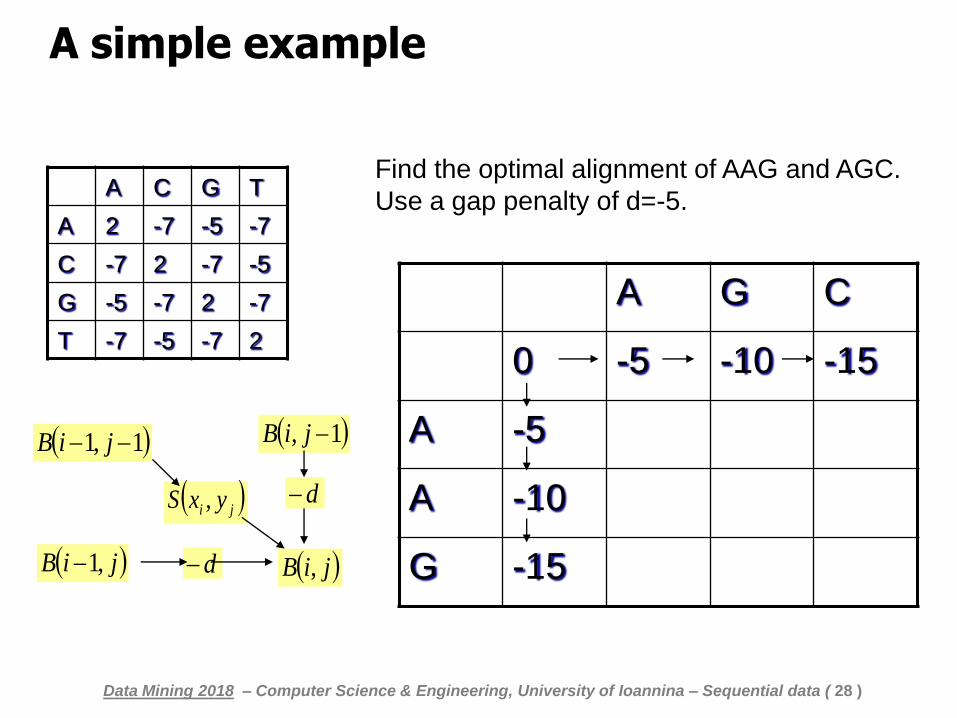
djiBdjiByxSjiBjiB ji 1,,,1,,1,1max,
Data Mining 2018 – Computer Science & Engineering, University of Ioannina – Sequential data ( 25 )
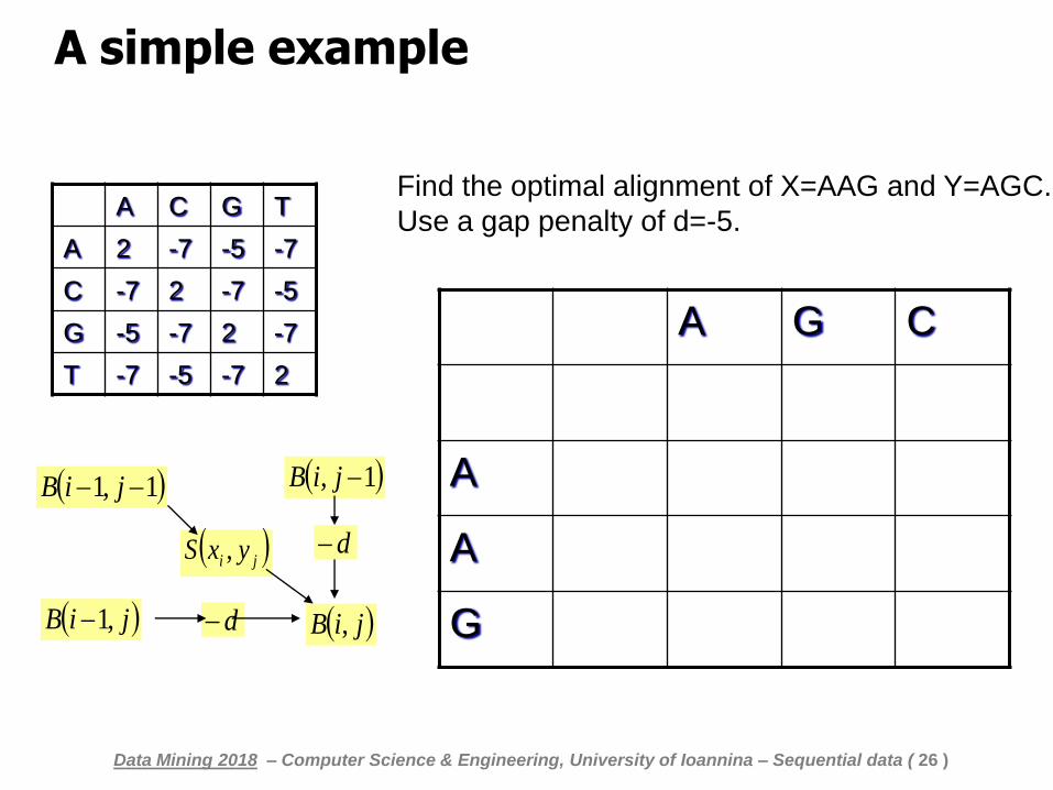
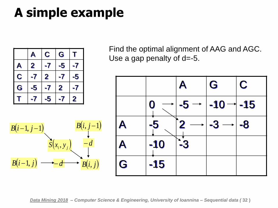
A simple example
A C G T
A 2 -7 -5 -7
C -7 2 -7 -5
G -5 -7 2 -7
T -7 -5 -7 2
A G C
A
A
G
1,1 jiB
jiB , jiB ,1
1, jiB
d
d ji yxS ,
Find the optimal alignment of X=AAG and Y=AGC.
Use a gap penalty of d=-5.
Data Mining 2018 – Computer Science & Engineering, University of Ioannina – Sequential data ( 26 )
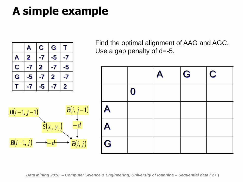
A simple example
A C G T
A 2 -7 -5 -7
C -7 2 -7 -5
G -5 -7 2 -7
T -7 -5 -7 2
A G C
0
A
A
G
1,1 jiB
jiB , jiB ,1
1, jiB
d
d ji yxS ,
Find the optimal alignment of AAG and AGC.
Use a gap penalty of d=-5.
Data Mining 2018 – Computer Science & Engineering, University of Ioannina – Sequential data ( 27 )
A simple example
A C G T
A 2 -7 -5 -7
C -7 2 -7 -5
G -5 -7 2 -7
T -7 -5 -7 2
A G C
0 -5 -10 -15
A -5
A -10
G -15
Find the optimal alignment of AAG and AGC.
Use a gap penalty of d=-5.
1,1 jiB
jiB , jiB ,1
1, jiB
d
d ji yxS ,
Data Mining 2018 – Computer Science & Engineering, University of Ioannina – Sequential data ( 28 )
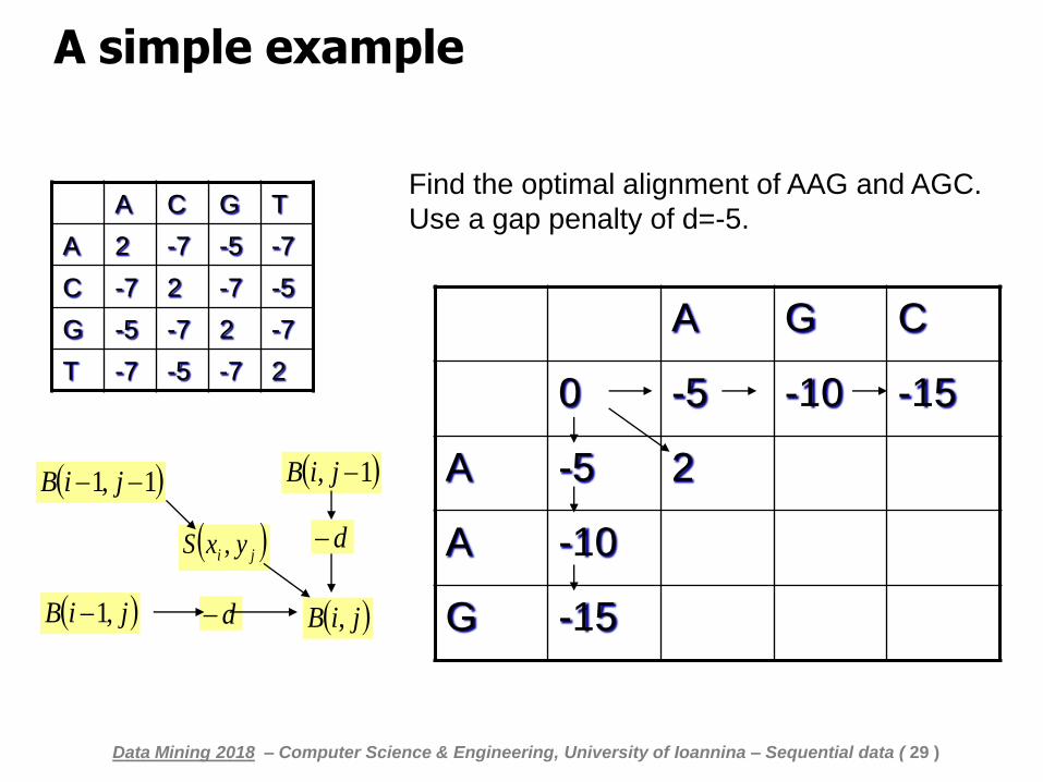
A simple example
A C G T
A 2 -7 -5 -7
C -7 2 -7 -5
G -5 -7 2 -7
T -7 -5 -7 2
A G C
0 -5 -10 -15
A -5 2
A -10
G -15
1,1 jiB
jiB , jiB ,1
1, jiB
d
d ji yxS ,
Find the optimal alignment of AAG and AGC.
Use a gap penalty of d=-5.
Data Mining 2018 – Computer Science & Engineering, University of Ioannina – Sequential data ( 29 )
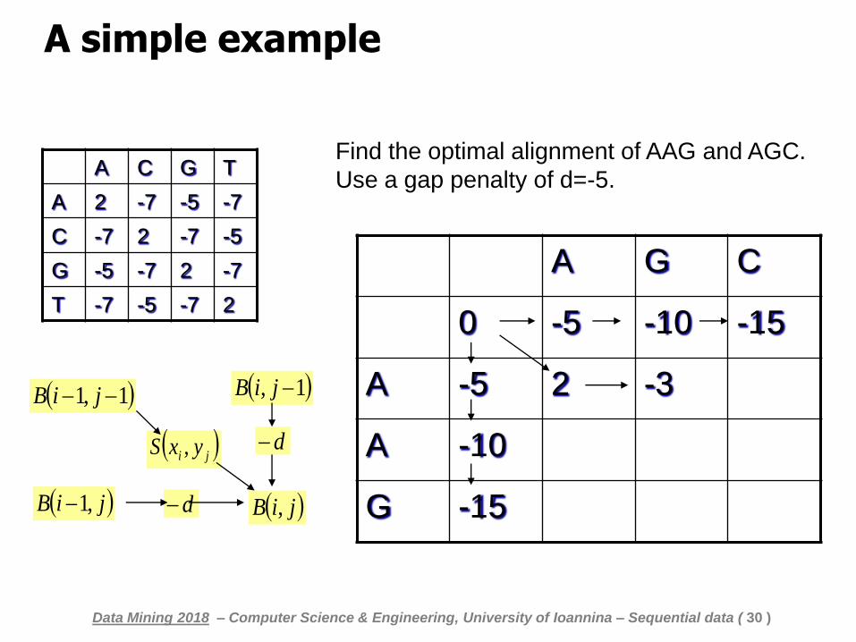
A simple example
A C G T
A 2 -7 -5 -7
C -7 2 -7 -5
G -5 -7 2 -7
T -7 -5 -7 2
A G C
0 -5 -10 -15
A -5 2 -3
A -10
G -15
1,1 jiB
jiB , jiB ,1
1, jiB
d
d ji yxS ,
Find the optimal alignment of AAG and AGC.
Use a gap penalty of d=-5.
Data Mining 2018 – Computer Science & Engineering, University of Ioannina – Sequential data ( 30 )
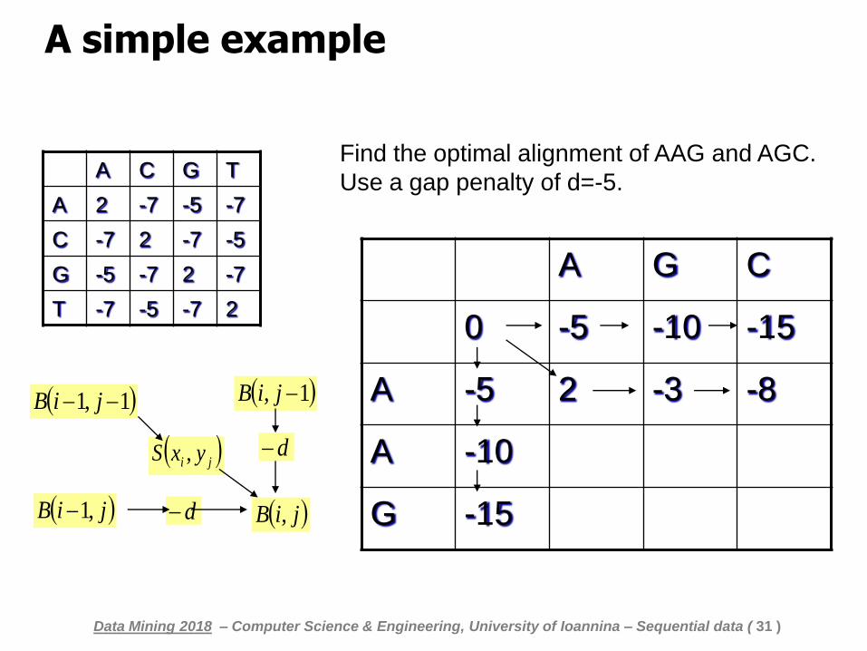
A simple example
A C G T
A 2 -7 -5 -7
C -7 2 -7 -5
G -5 -7 2 -7
T -7 -5 -7 2
A G C
0 -5 -10 -15
A -5 2 -3 -8
A -10
G -15
1,1 jiB
jiB , jiB ,1
1, jiB
d
d ji yxS ,
Find the optimal alignment of AAG and AGC.
Use a gap penalty of d=-5.
Data Mining 2018 – Computer Science & Engineering, University of Ioannina – Sequential data ( 31 )
A simple example
A C G T
A 2 -7 -5 -7
C -7 2 -7 -5
G -5 -7 2 -7
T -7 -5 -7 2
A G C
0 -5 -10 -15
A -5 2 -3 -8
A -10 -3
G -15
1,1 jiB
jiB , jiB ,1
1, jiB
d
d ji yxS ,
Find the optimal alignment of AAG and AGC.
Use a gap penalty of d=-5.
Data Mining 2018 – Computer Science & Engineering, University of Ioannina – Sequential data ( 32 )

A simple example
A C G T
A 2 -7 -5 -7
C -7 2 -7 -5
G -5 -7 2 -7
T -7 -5 -7 2
A G C
0 -5 -10 -15
A -5 2 -3 -8
A -10 -3
G -15 -8
1,1 jiB
jiB , jiB ,1
1, jiB
d
d ji yxS ,
Find the optimal alignment of AAG and AGC.
Use a gap penalty of d=-5.
Data Mining 2018 – Computer Science & Engineering, University of Ioannina – Sequential data ( 33 )

A simple example
A C G T
A 2 -7 -5 -7
C -7 2 -7 -5
G -5 -7 2 -7
T -7 -5 -7 2
A G C
0 -5 -10 -15
A -5 2 -3 -8
A -10 -3 -3
G -15 -8
1,1 jiB
jiB , jiB ,1
1, jiB
d
d ji yxS ,
Find the optimal alignment of AAG and AGC.
Use a gap penalty of d=-5.
Data Mining 2018 – Computer Science & Engineering, University of Ioannina – Sequential data ( 34 )

A simple example
A C G T
A 2 -7 -5 -7
C -7 2 -7 -5
G -5 -7 2 -7
T -7 -5 -7 2
A G C
0 -5 -10 -15
A -5 2 -3 -8
A -10 -3 -3 -8
G -15 -8
1,1 jiB
jiB , jiB ,1
1, jiB
d
d ji yxS ,
Find the optimal alignment of AAG and AGC.
Use a gap penalty of d=-5.
Data Mining 2018 – Computer Science & Engineering, University of Ioannina – Sequential data ( 35 )

A simple example
A C G T
A 2 -7 -5 -7
C -7 2 -7 -5
G -5 -7 2 -7
T -7 -5 -7 2
A G C
0 -5 -10 -15
A -5 2 -3 -8
A -10 -3 -3 -8
G -15 -8 -1
1,1 jiB
jiB , jiB ,1
1, jiB
d
d ji yxS ,
Find the optimal alignment of AAG and AGC.
Use a gap penalty of d=-5.
Data Mining 2018 – Computer Science & Engineering, University of Ioannina – Sequential data ( 36 )
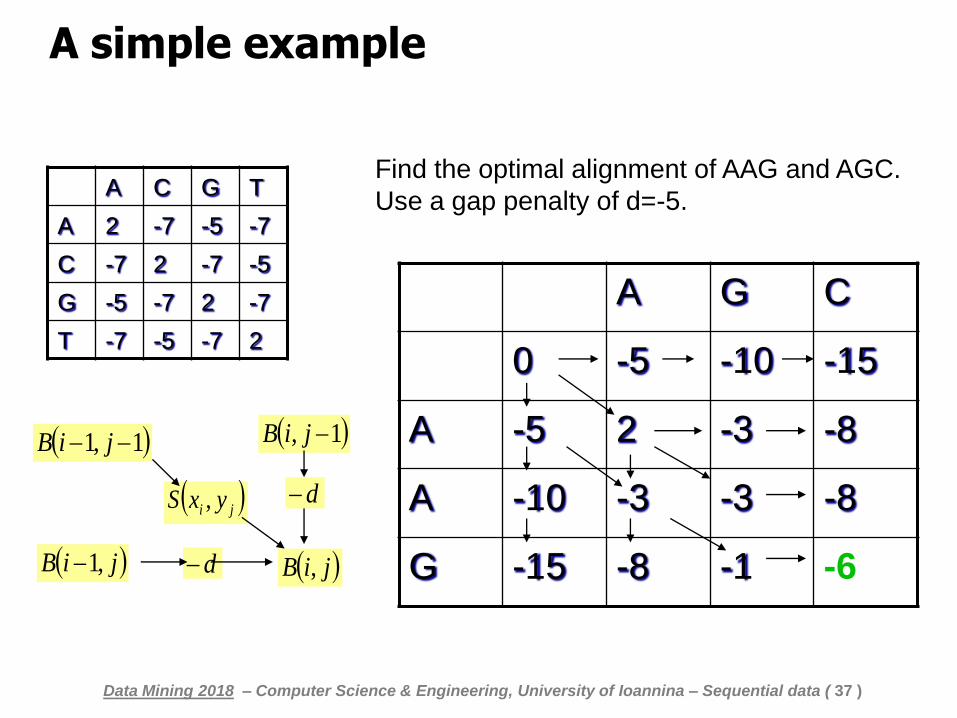
A simple example
A C G T
A 2 -7 -5 -7
C -7 2 -7 -5
G -5 -7 2 -7
T -7 -5 -7 2
A G C
0 -5 -10 -15
A -5 2 -3 -8
A -10 -3 -3 -8
G -15 -8 -1 -6
1,1 jiB
jiB , jiB ,1
1, jiB
d
d ji yxS ,
Find the optimal alignment of AAG and AGC.
Use a gap penalty of d=-5.
Data Mining 2018 – Computer Science & Engineering, University of Ioannina – Sequential data ( 37 )
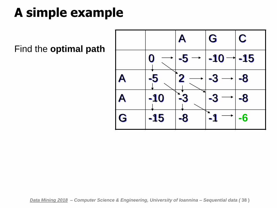
A simple example
Find the optimal path
Data Mining 2018 – Computer Science & Engineering, University of Ioannina – Sequential data ( 38 )
A G C
0 -5 -10 -15
A -5 2 -3 -8
A -10 -3 -3 -8
G -15 -8 -1 -6
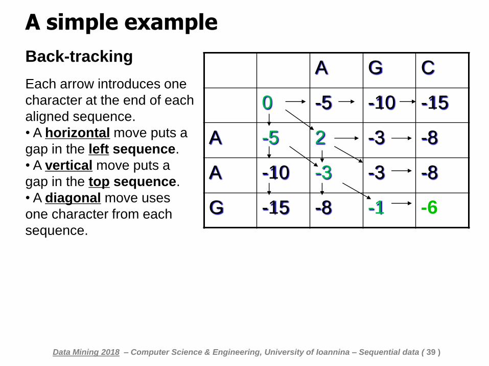
A simple example
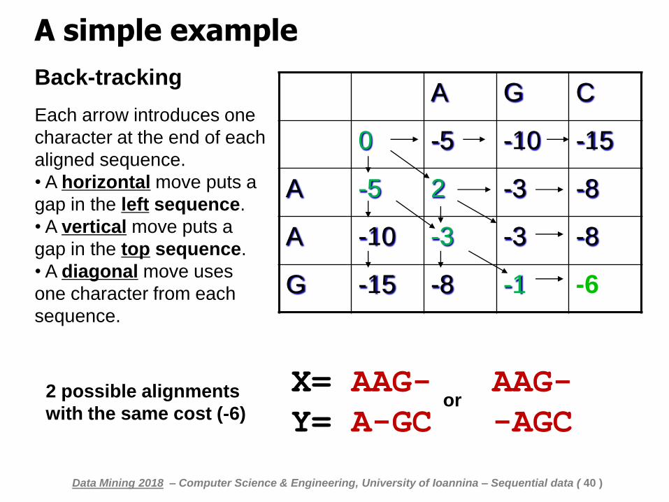
Back-tracking
Each arrow introduces one
character at the end of each
aligned sequence.
• A horizontal move puts a
gap in the left sequence.
• A vertical move puts a
gap in the top sequence.
• A diagonal move uses
one character from each
sequence.
Data Mining 2018 – Computer Science & Engineering, University of Ioannina – Sequential data ( 39 )
A G C
0 -5 -10 -15
A -5 2 -3 -8
A -10 -3 -3 -8
G -15 -8 -1 -6
A simple example
Back-tracking
Each arrow introduces one
character at the end of each
aligned sequence.
• A horizontal move puts a
gap in the left sequence.
• A vertical move puts a
gap in the top sequence.
• A diagonal move uses
one character from each
sequence.
X= AAG- AAG-
Y= A-GC -AGC 2 possible alignments
with the same cost (-6) or
Data Mining 2018 – Computer Science & Engineering, University of Ioannina – Sequential data ( 40 )
A G C
0 -5 -10 -15
A -5 2 -3 -8
A -10 -3 -3 -8
G -15 -8 -1 -6
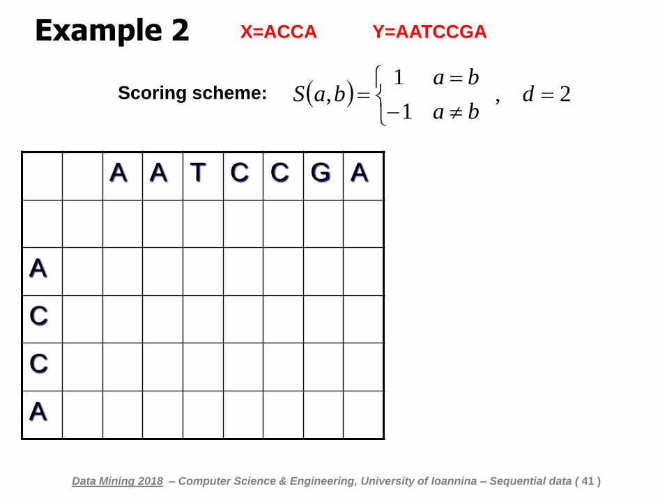
Example 2
A A T C C G A
A
C
C
A
Scoring scheme: 2 , 1
1,
d
ba
babaS
Data Mining 2018 – Computer Science & Engineering, University of Ioannina – Sequential data ( 41 )
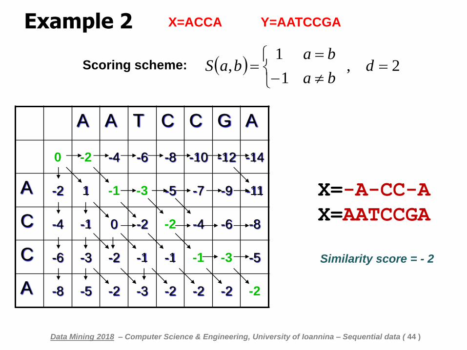
X=ACCA Y=AATCCGA
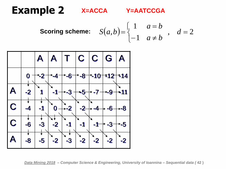
Example 2
A A T C C G A
0 -2 -4 -6 -8 -10 -12 -14
A -2 1 -1 -3 -5 -7 -9 -11
C -4 -1 0 -2 -2 -4 -6 -8
C -6 -3 -2 -1 -1 -1 -3 -5
A -8 -5 -2 -3 -2 -2 -2 -2
Scoring scheme: 2 , 1
1,
d
ba
babaS
X=ACCA Y=AATCCGA
Data Mining 2018 – Computer Science & Engineering, University of Ioannina – Sequential data ( 42 )
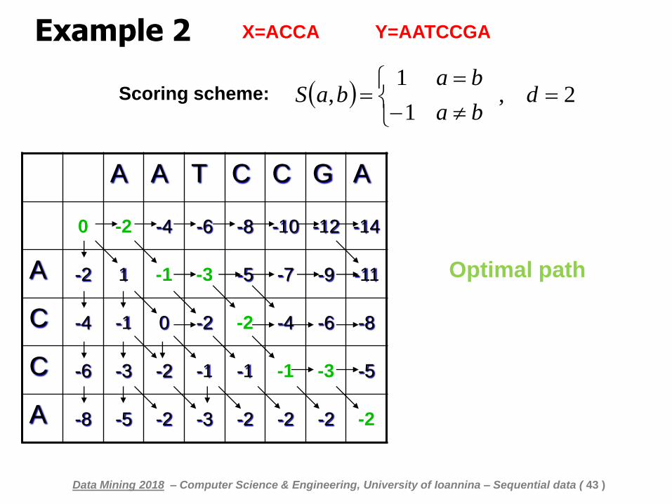
Example 2
A A T C C G A
0 -2 -4 -6 -8 -10 -12 -14
A -2 1 -1 -3 -5 -7 -9 -11
C -4 -1 0 -2 -2 -4 -6 -8
C -6 -3 -2 -1 -1 -1 -3 -5
A -8 -5 -2 -3 -2 -2 -2 -2
Scoring scheme: 2 , 1
1,
d
ba
babaS
Optimal path
Data Mining 2018 – Computer Science & Engineering, University of Ioannina – Sequential data ( 43 )
X=ACCA Y=AATCCGA
Example 2
A A T C C G A
0 -2 -4 -6 -8 -10 -12 -14
A -2 1 -1 -3 -5 -7 -9 -11
C -4 -1 0 -2 -2 -4 -6 -8
C -6 -3 -2 -1 -1 -1 -3 -5
A -8 -5 -2 -3 -2 -2 -2 -2
Scoring scheme: 2 , 1
1,
d
ba
babaS
X=-A-CC-A
Χ=AATCCGA
Similarity score = - 2
Data Mining 2018 – Computer Science & Engineering, University of Ioannina – Sequential data ( 44 )
X=ACCA Y=AATCCGA
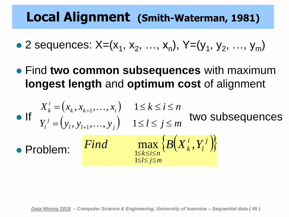
Local Alignment (Smith-Waterman, 1981)
2 sequences: X=(x1, x2, …, xn), Y=(y1, y2, …, ym)
Find two common subsequences with maximum
longest length and optimum cost of alignment
If two subsequences
Problem:
mjlyyyY
nikxxxX
jll
j
l
ikk
i
k
1 ,,,
1 ,,,
1
1
j
l
i
k
mjlnik
YXBFind ,max
11
Data Mining 2018 – Computer Science & Engineering, University of Ioannina – Sequential data ( 45 )
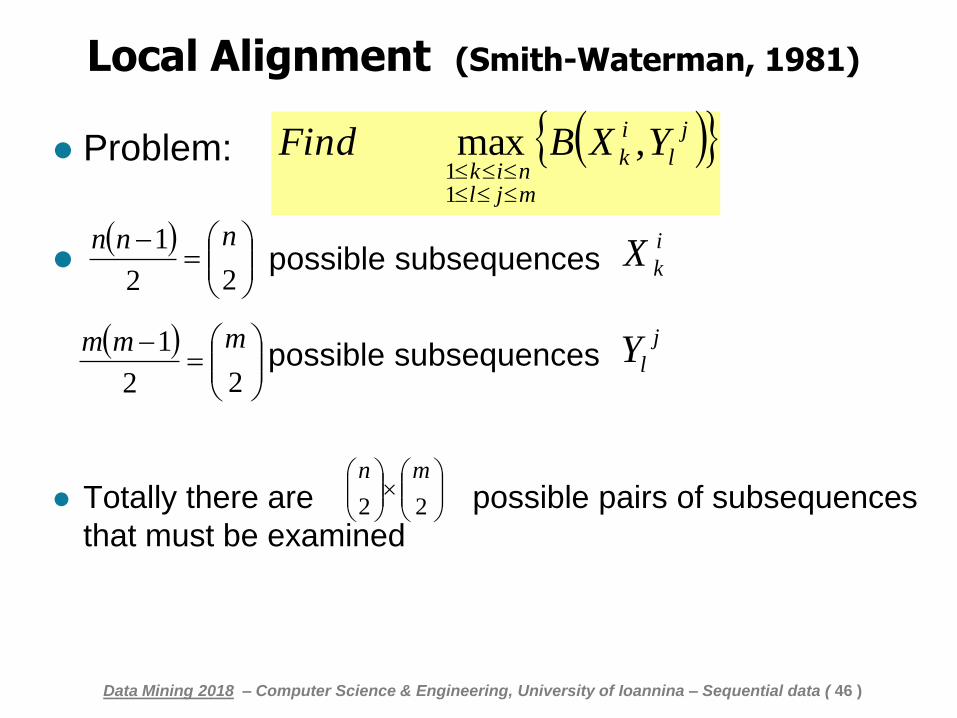
Local Alignment (Smith-Waterman, 1981)
Problem:
possible subsequences
possible subsequences
Totally there are possible pairs of subsequences
that must be examined
j
l
i
k
mjlnik
YXBFind ,max
11
22
1 nnn i
kX
22
1 mmm j
lY
22
mn
Data Mining 2018 – Computer Science & Engineering, University of Ioannina – Sequential data ( 46 )
Local Alignment (Smith-Waterman, 1981)
Dynamic programming to solve this problem
Introduce a score function L(i,j) and consider a
(supposed) starting point I, where L(I)=0.
L(i,j) denotes the maximum total score all paths
starting from I and ending at (i,j).
Then there are four (4) cases:
Data Mining 2018 – Computer Science & Engineering, University of Ioannina – Sequential data ( 47 )
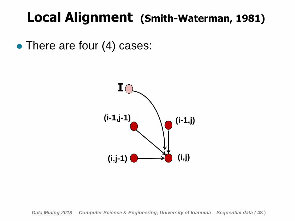
Local Alignment (Smith-Waterman, 1981)
Τhere are four (4) cases:
(i-1,j-1)
(i,j)
(i-1,j)
(i,j-1)
I
Data Mining 2018 – Computer Science & Engineering, University of Ioannina – Sequential data ( 48 )
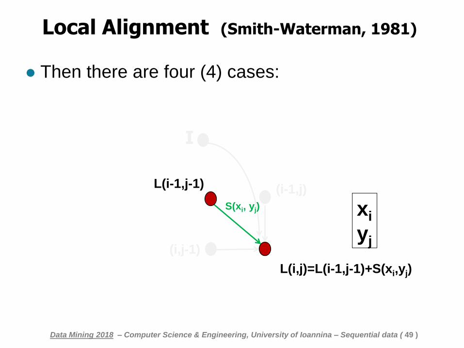
Local Alignment (Smith-Waterman, 1981)
Then there are four (4) cases:
L(i-1,j-1) (i-1,j)
(i,j-1)
I
L(i,j)=L(i-1,j-1)+S(xi,yj)
xi
yj
S(xi, yj)
Data Mining 2018 – Computer Science & Engineering, University of Ioannina – Sequential data ( 49 )
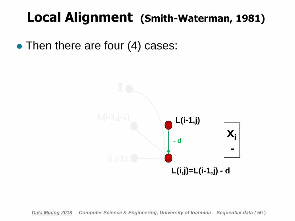
Local Alignment (Smith-Waterman, 1981)
Then there are four (4) cases:
L(i-1,j-1) L(i-1,j)
(i,j-1)
I
L(i,j)=L(i-1,j) - d
xi
- - d
Data Mining 2018 – Computer Science & Engineering, University of Ioannina – Sequential data ( 50 )
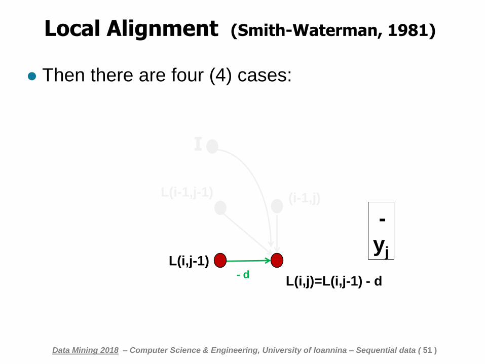
Local Alignment (Smith-Waterman, 1981)
Then there are four (4) cases:
L(i-1,j-1) (i-1,j)
L(i,j-1)
I
L(i,j)=L(i,j-1) - d
-
yj
- d
Data Mining 2018 – Computer Science & Engineering, University of Ioannina – Sequential data ( 51 )
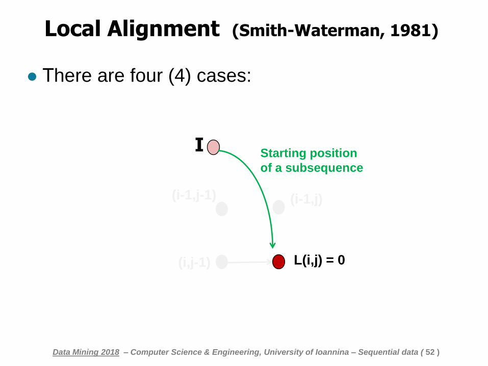
Local Alignment (Smith-Waterman, 1981)
Τhere are four (4) cases:
(i-1,j-1)
L(i,j) = 0
(i-1,j)
(i,j-1)
I Starting position
of a subsequence
Data Mining 2018 – Computer Science & Engineering, University of Ioannina – Sequential data ( 52 )
Local Alignment (Smith-Waterman, 1981)
Problem: Longest Common Subsequence
Cost function L(i,j) , 0 ≤ i ≤ n , 0 ≤ j ≤ m
Data Mining 2018 – Computer Science & Engineering, University of Ioannina – Sequential data ( 53 )
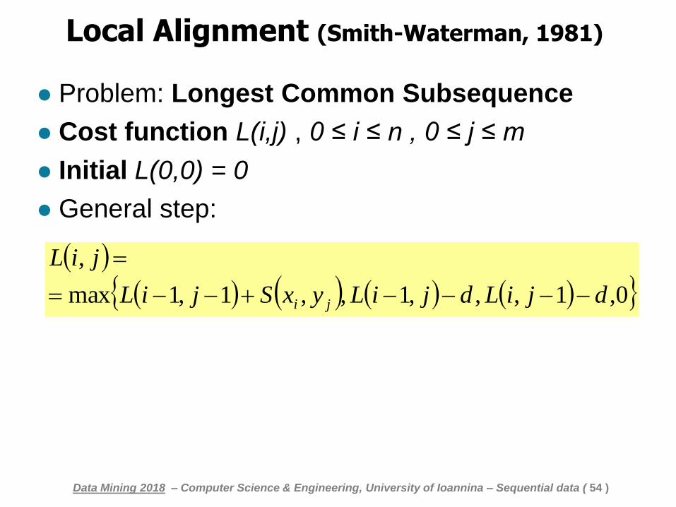
Local Alignment (Smith-Waterman, 1981)
Problem: Longest Common Subsequence
Cost function L(i,j) , 0 ≤ i ≤ n , 0 ≤ j ≤ m
Initial L(0,0) = 0
General step:
0,1,,,1,,1,1max
,
djiLdjiLyxSjiL
jiL
ji
Data Mining 2018 – Computer Science & Engineering, University of Ioannina – Sequential data ( 54 )
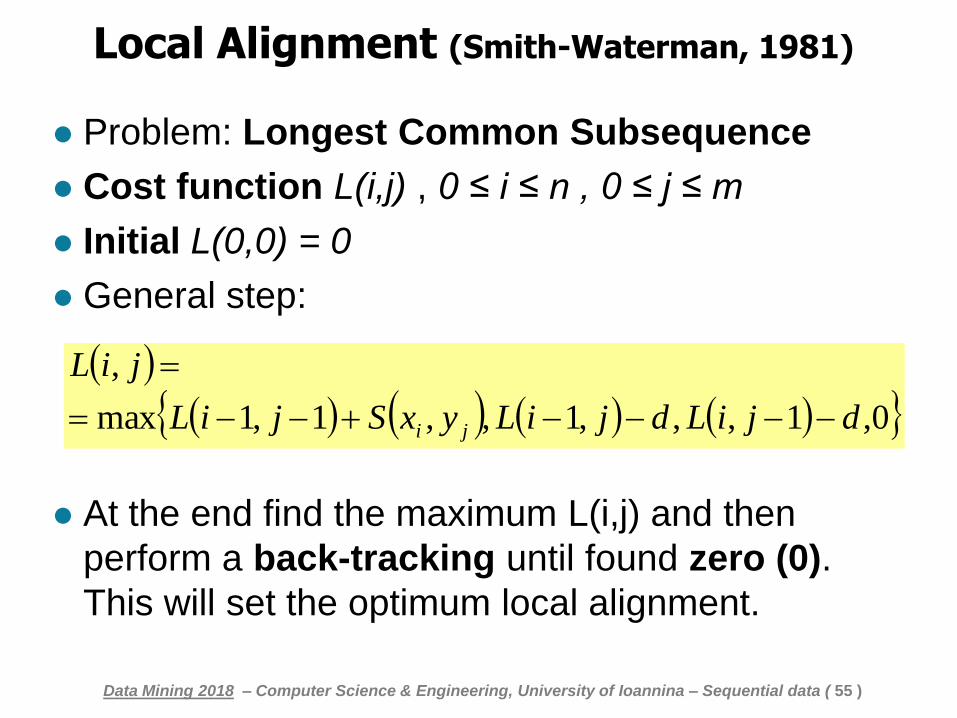
Local Alignment (Smith-Waterman, 1981)
Problem: Longest Common Subsequence
Cost function L(i,j) , 0 ≤ i ≤ n , 0 ≤ j ≤ m
Initial L(0,0) = 0
General step:
At the end find the maximum L(i,j) and then
perform a back-tracking until found zero (0).
This will set the optimum local alignment.
0,1,,,1,,1,1max
,
djiLdjiLyxSjiL
jiL
ji
Data Mining 2018 – Computer Science & Engineering, University of Ioannina – Sequential data ( 55 )
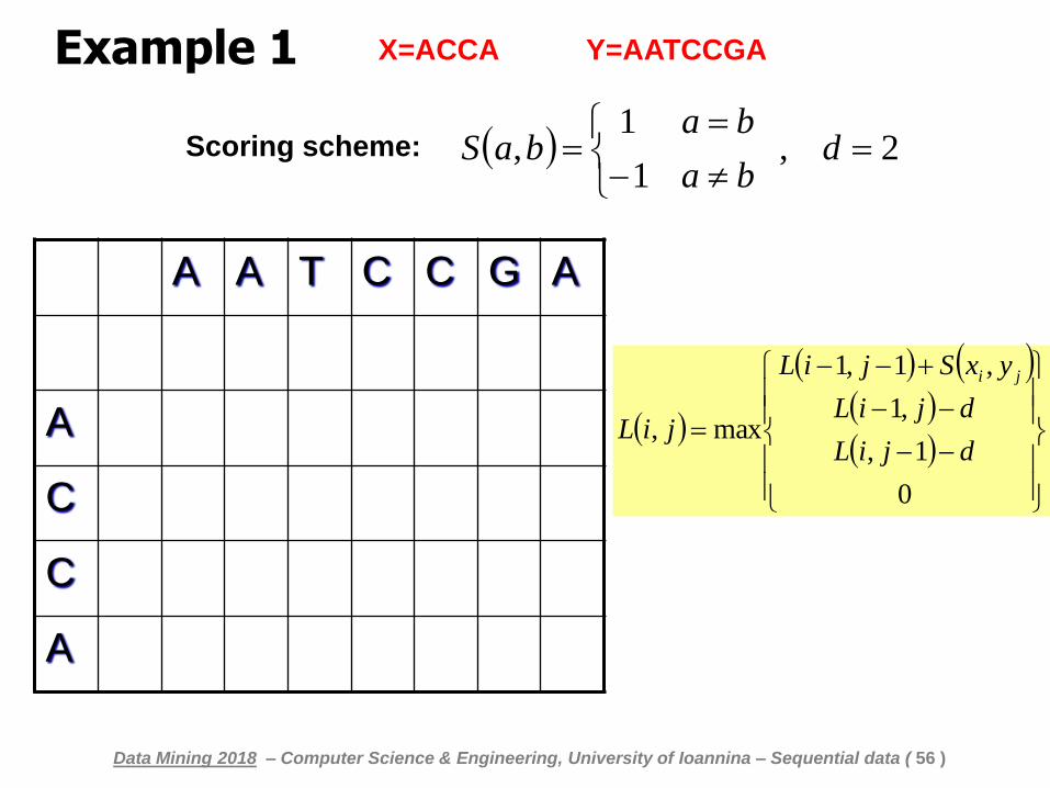
Example 1
A A T C C G A
A
C
C
A
Scoring scheme: 2 , 1
1,
d
ba
babaS
0
1,
,1
,1,1
max,djiL
djiL
yxSjiL
jiL
ji
Data Mining 2018 – Computer Science & Engineering, University of Ioannina – Sequential data ( 56 )
X=ACCA Y=AATCCGA
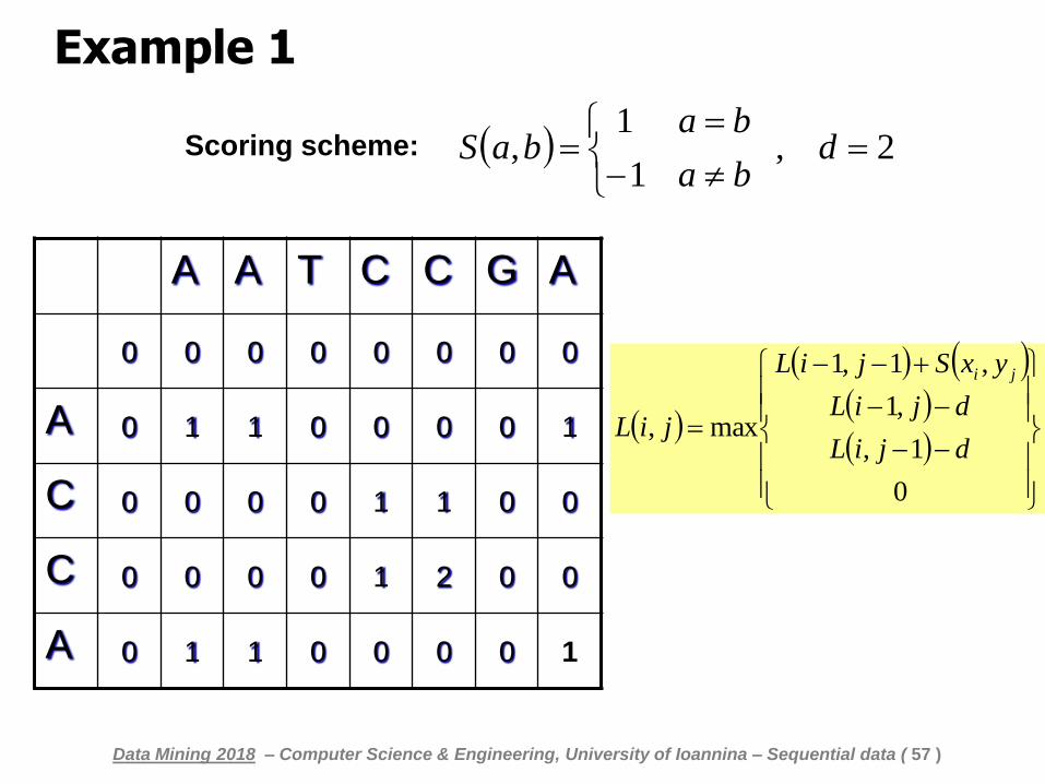
Example 1
A A T C C G A
0 0 0 0 0 0 0 0
A 0 1 1 0 0 0 0 1
C 0 0 0 0 1 1 0 0
C 0 0 0 0 1 2 0 0
A 0 1 1 0 0 0 0 1
Scoring scheme: 2 , 1
1,
d
ba
babaS
0
1,
,1
,1,1
max,djiL
djiL
yxSjiL
jiL
ji
Data Mining 2018 – Computer Science & Engineering, University of Ioannina – Sequential data ( 57 )
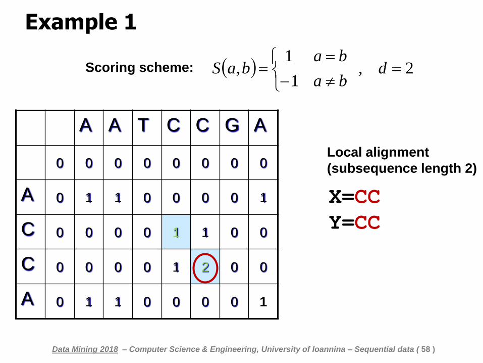
Example 1
A A T C C G A
0 0 0 0 0 0 0 0
A 0 1 1 0 0 0 0 1
C 0 0 0 0 1 1 0 0
C 0 0 0 0 1 2 0 0
A 0 1 1 0 0 0 0 1
Scoring scheme: 2 , 1
1,
d
ba
babaS
Χ=CC
Υ=CC
Local alignment
(subsequence length 2)
Data Mining 2018 – Computer Science & Engineering, University of Ioannina – Sequential data ( 58 )
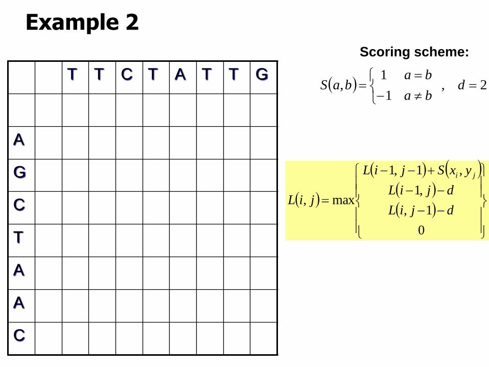
Example 2
T T C T A T T G
A
G
C
T
A
A
C
Scoring scheme:
2 , 1
1,
d
ba
babaS
0
1,
,1
,1,1
max,djiL
djiL
yxSjiL
jiL
ji
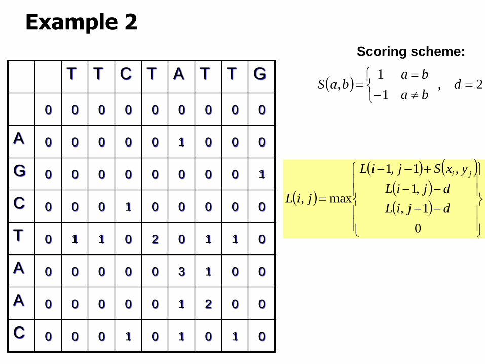
Example 2
T T C T A T T G
0 0 0 0 0 0 0 0 0
A 0 0 0 0 0 1 0 0 0
G 0 0 0 0 0 0 0 0 1
C 0 0 0 1 0 0 0 0 0
T 0 1 1 0 2 0 1 1 0
A 0 0 0 0 0 3 1 0 0
A 0 0 0 0 0 1 2 0 0
C 0 0 0 1 0 1 0 1 0
Scoring scheme:
2 , 1
1,
d
ba
babaS
0
1,
,1
,1,1
max,djiL
djiL
yxSjiL
jiL
ji
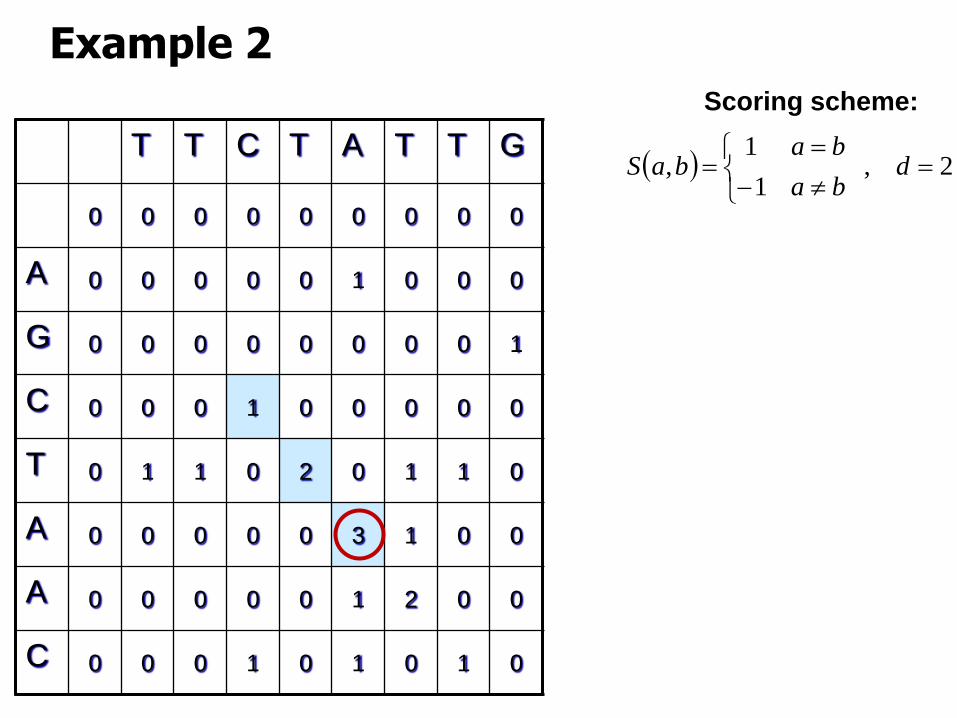
Example 2
T T C T A T T G
0 0 0 0 0 0 0 0 0
A 0 0 0 0 0 1 0 0 0
G 0 0 0 0 0 0 0 0 1
C 0 0 0 1 0 0 0 0 0
T 0 1 1 0 2 0 1 1 0
A 0 0 0 0 0 3 1 0 0
A 0 0 0 0 0 1 2 0 0
C 0 0 0 1 0 1 0 1 0
Scoring scheme:
2 , 1
1,
d
ba
babaS
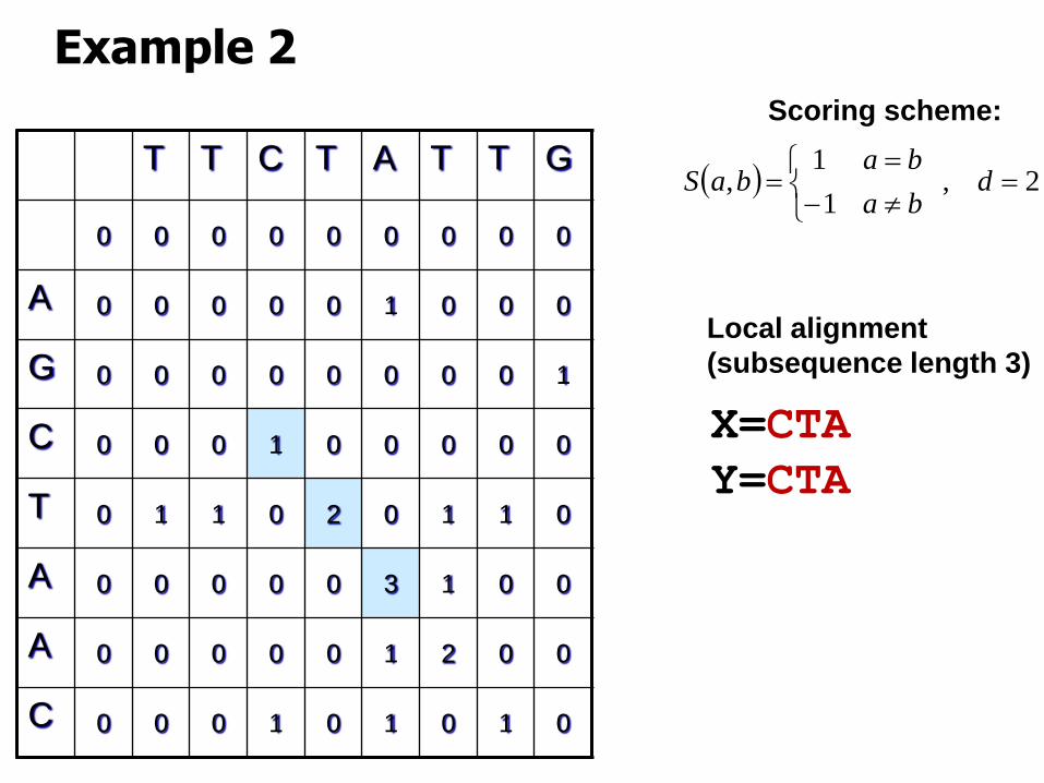
Example 2
T T C T A T T G
0 0 0 0 0 0 0 0 0
A 0 0 0 0 0 1 0 0 0
G 0 0 0 0 0 0 0 0 1
C 0 0 0 1 0 0 0 0 0
T 0 1 1 0 2 0 1 1 0
A 0 0 0 0 0 3 1 0 0
A 0 0 0 0 0 1 2 0 0
C 0 0 0 1 0 1 0 1 0
Scoring scheme:
2 , 1
1,
d
ba
babaS
Χ=CTA
Υ=CTA
Local alignment
(subsequence length 3)
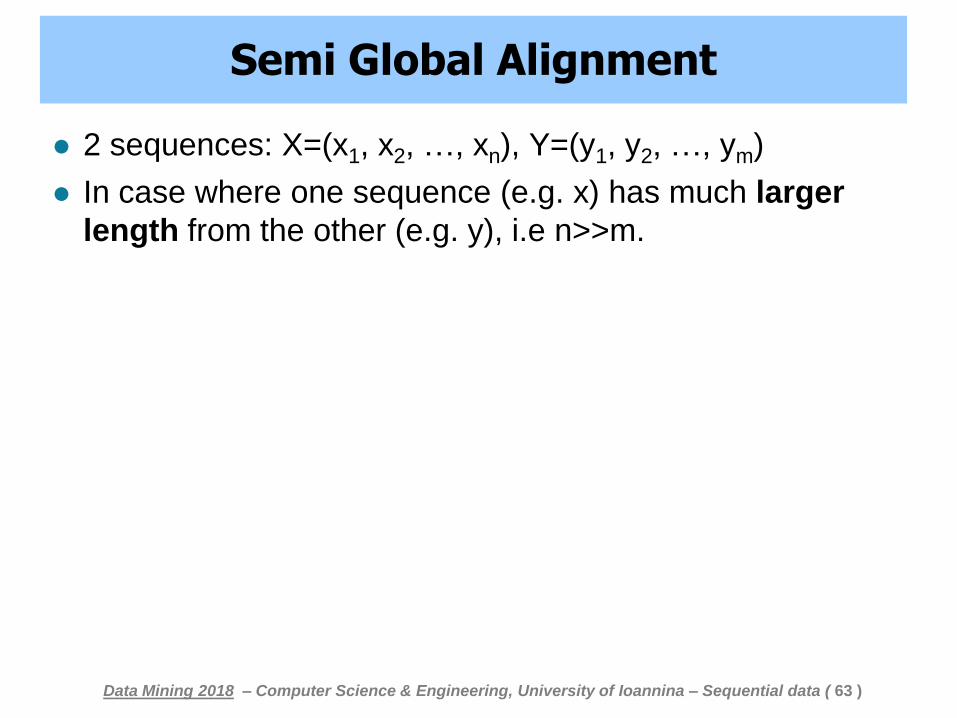
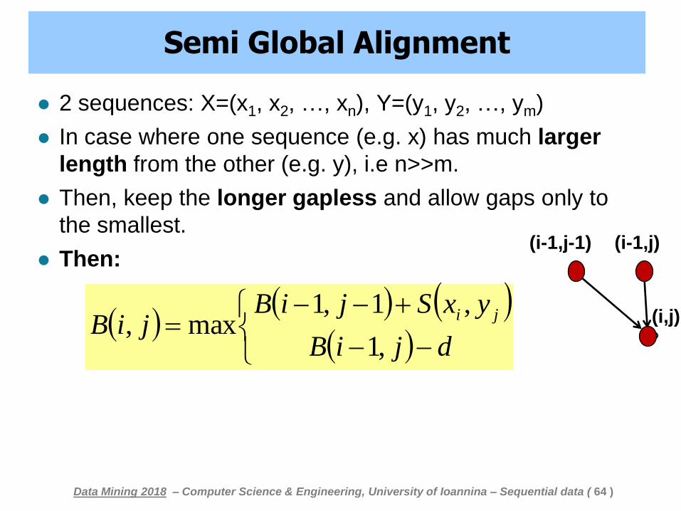
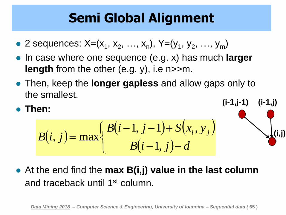
Semi Global Alignment
2 sequences: X=(x1, x2, …, xn), Y=(y1, y2, …, ym)
In case where one sequence (e.g. x) has much larger
length from the other (e.g. y), i.e n>>m.
Then, keep the longer gapless and allow gaps only to
the smallest.
Then:
At the end find the max B(i,j) value in the last column
and traceback until 1st column.
djiB
yxSjiBjiB
ji
,1
,1,1max,
(i-1,j-1)
(i,j)
(i-1,j)
Data Mining 2018 – Computer Science & Engineering, University of Ioannina – Sequential data ( 63 )
Semi Global Alignment
2 sequences: X=(x1, x2, …, xn), Y=(y1, y2, …, ym)
In case where one sequence (e.g. x) has much larger
length from the other (e.g. y), i.e n>>m.
Then, keep the longer gapless and allow gaps only to
the smallest.
Then:
At the end find the max B(i,j) value in the last column
and traceback until 1st column.
djiB
yxSjiBjiB
ji
,1
,1,1max,
(i-1,j-1)
(i,j)
(i-1,j)
Data Mining 2018 – Computer Science & Engineering, University of Ioannina – Sequential data ( 64 )
Semi Global Alignment
2 sequences: X=(x1, x2, …, xn), Y=(y1, y2, …, ym)
In case where one sequence (e.g. x) has much larger
length from the other (e.g. y), i.e n>>m.
Then, keep the longer gapless and allow gaps only to
the smallest.
Then:
At the end find the max B(i,j) value in the last column
and traceback until 1st column.
djiB
yxSjiBjiB
ji
,1
,1,1max,
(i-1,j-1)
(i,j)
(i-1,j)
Data Mining 2018 – Computer Science & Engineering, University of Ioannina – Sequential data ( 65 )
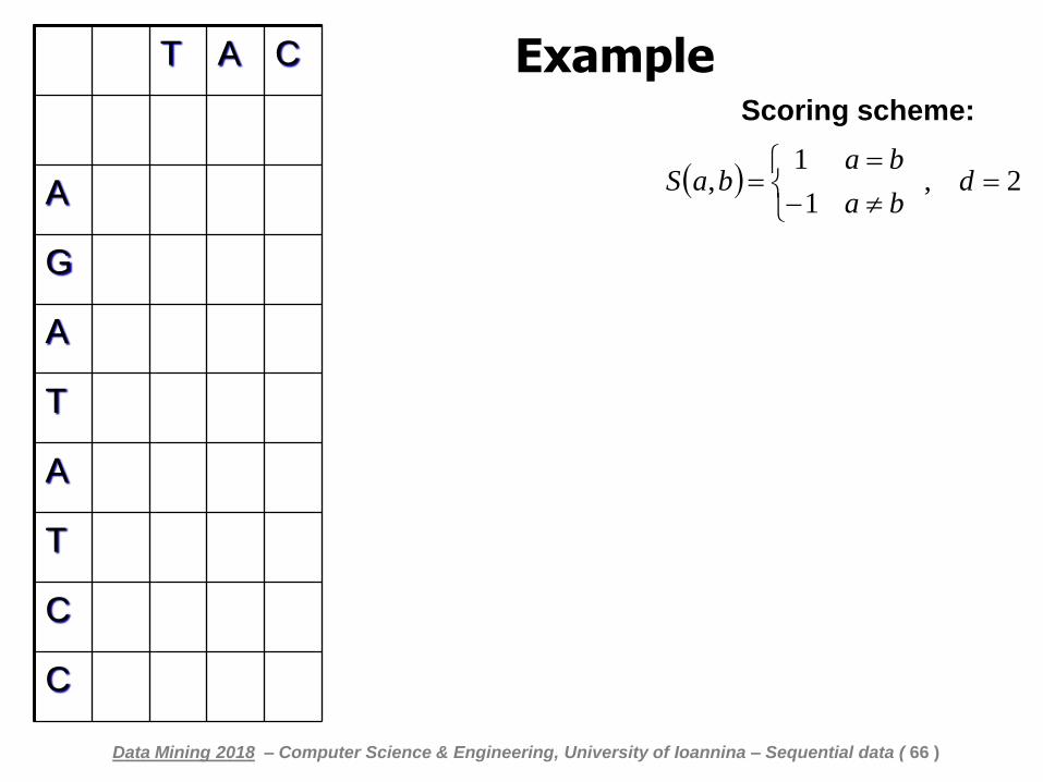
Example T A C
A
G
A
T
A
T
C
C
Scoring scheme:
2 , 1
1,
d
ba
babaS
Data Mining 2018 – Computer Science & Engineering, University of Ioannina – Sequential data ( 66 )
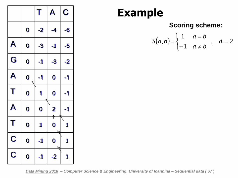
Example T A C
0 -2 -4 -6
A 0 -3 -1 -5
G 0 -1 -3 -2
A 0 -1 0 -1
T 0 1 0 -1
A 0 0 2 -1
T 0 1 0 1
C 0 -1 0 1
C 0 -1 -2 1
Scoring scheme:
2 , 1
1,
d
ba
babaS
Data Mining 2018 – Computer Science & Engineering, University of Ioannina – Sequential data ( 67 )
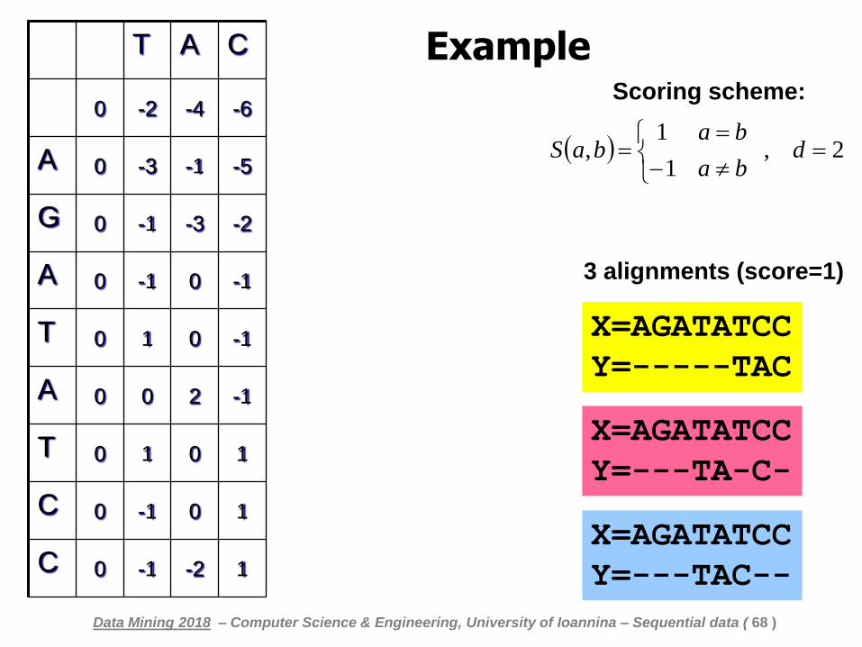
Example T A C
0 -2 -4 -6
A 0 -3 -1 -5
G 0 -1 -3 -2
A 0 -1 0 -1
T 0 1 0 -1
A 0 0 2 -1
T 0 1 0 1
C 0 -1 0 1
C 0 -1 -2 1
Scoring scheme:
2 , 1
1,
d
ba
babaS
Data Mining 2018 – Computer Science & Engineering, University of Ioannina – Sequential data ( 68 )
Χ=AGATATCC
Υ=-----TAC
3 alignments (score=1)
Χ=AGATATCC
Υ=---TA-C-
Χ=AGATATCC
Υ=---TAC--
Data Mining 2018 – Computer Science & Engineering, University of Ioannina – Sequential data ( 69 )
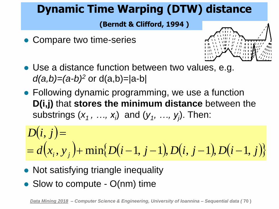
Dynamic Time Warping (DTW) distance
(Berndt & Clifford, 1994 )
Compare two time-series
Use a distance function between two values, e.g.
d(a,b)=(a-b)2 or d(a,b)=|a-b|
Following dynamic programming, we use a function
D(i,j) that stores the minimum distance between the
substrings (x1 , …, xi) and (y1, …, yj). Then:
Not satisfying triangle inequality
Slow to compute - O(nm) time
jiDjiDjiDyxd
jiD
ji ,1,1,,1,1min,
,
Data Mining 2018 – Computer Science & Engineering, University of Ioannina – Sequential data ( 70 )
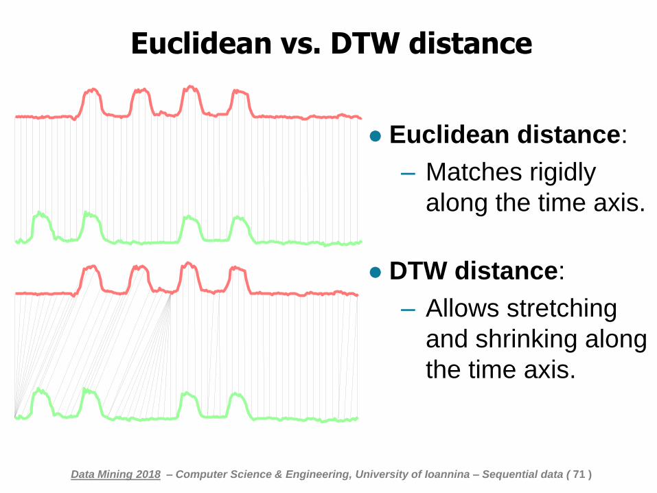
Euclidean vs. DTW distance
Euclidean distance:
– Matches rigidly
along the time axis.
DTW distance:
– Allows stretching
and shrinking along
the time axis.
Data Mining 2018 – Computer Science & Engineering, University of Ioannina – Sequential data ( 71 )
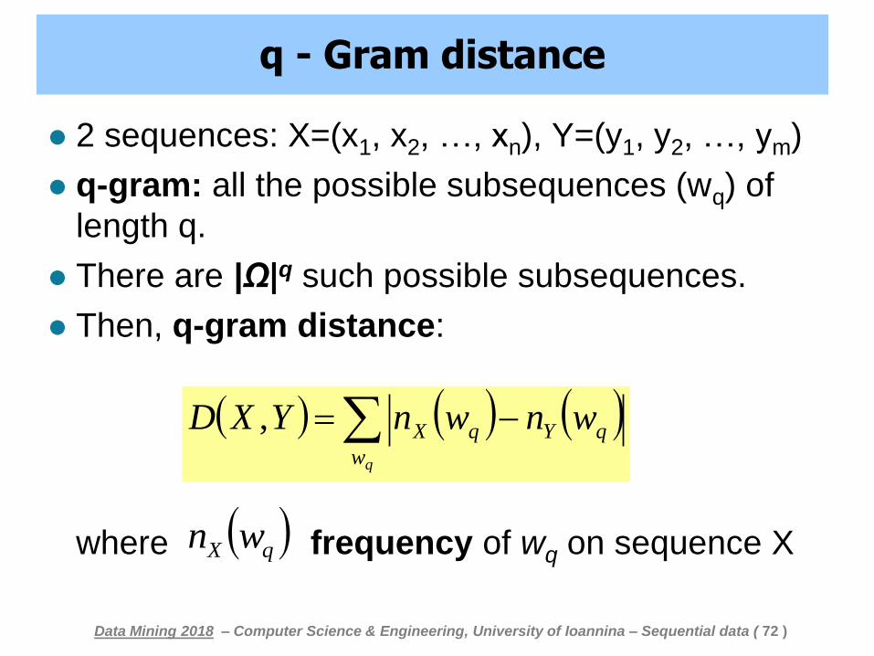
q - Gram distance
2 sequences: X=(x1, x2, …, xn), Y=(y1, y2, …, ym)
q-gram: all the possible subsequences (wq) of
length q.
There are |Ω|q such possible subsequences.
Then, q-gram distance:
where frequency of wq on sequence X
qw
qYqX wnwnYXD ,
qX wn
Data Mining 2018 – Computer Science & Engineering, University of Ioannina – Sequential data ( 72 )
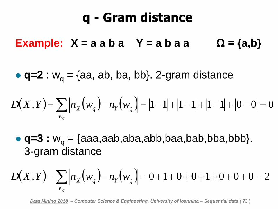
q - Gram distance
Example: X = a a b a Y = a b a a Ω = {a,b}
q=2 : wq = {aa, ab, ba, bb}. 2-gram distance
q=3 : wq = {aaa,aab,aba,abb,baa,bab,bba,bbb}.
3-gram distance
000111111, qw
qYqX wnwnYXD
200010010, qw
qYqX wnwnYXD
Data Mining 2018 – Computer Science & Engineering, University of Ioannina – Sequential data ( 73 )