Dirac-Hartree-Fock Theory

1

Hamiltonian of the complete system

(atom + radiation)

H = Hrad +Hel +Hint

Hrad =1

8π

∫

(E2 +H2)

Hint = −∑

k

ek(αkA(k))

Hel =∑

k

(αk · pk + βkmk)

Free atom or ion with no external fields:

Hrad = 0 , Hint << Hel

2

Schrodinger (Dirac) Wave Equation

HΨ = i ∂∂t

Ψ Time dependent

HΨ = EΨ Time independent

Ψ (r1, r2, . . . , rN , t) 3N+1 Variables

Ψ (r1, r2, . . . , rN ) 3N Variables

3

. . . The solution is a function of 3N variables,

even if it were possible to evaluate such a

solution to any degree of numerical accuracy

required, no satisfactory way of presenting the

results is known. . . . the full specification of a

single wave function of neutral Fe is a

function of seventy eight variables. It would

be rather crude to restrict to ten the number

of values of each variable at which to tabulate

this function, but even so, full tabulation of it

would require 10 78 entries, and even if this

number could be reduced somewhat from

considerations of symmetry, there would still

not be enough atoms in the whole solar

system to provide the material for printing

such a table. Hartree (1948)

4

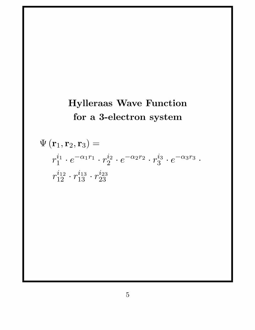
Hylleraas Wave Function

for a 3-electron system

Ψ(r1, r2, r3) =

ri11 · e−α1r1 · ri2

2 · e−α2r2 · ri33 · e−α3r3 ·

ri1212 · ri13

13 · ri2323

5

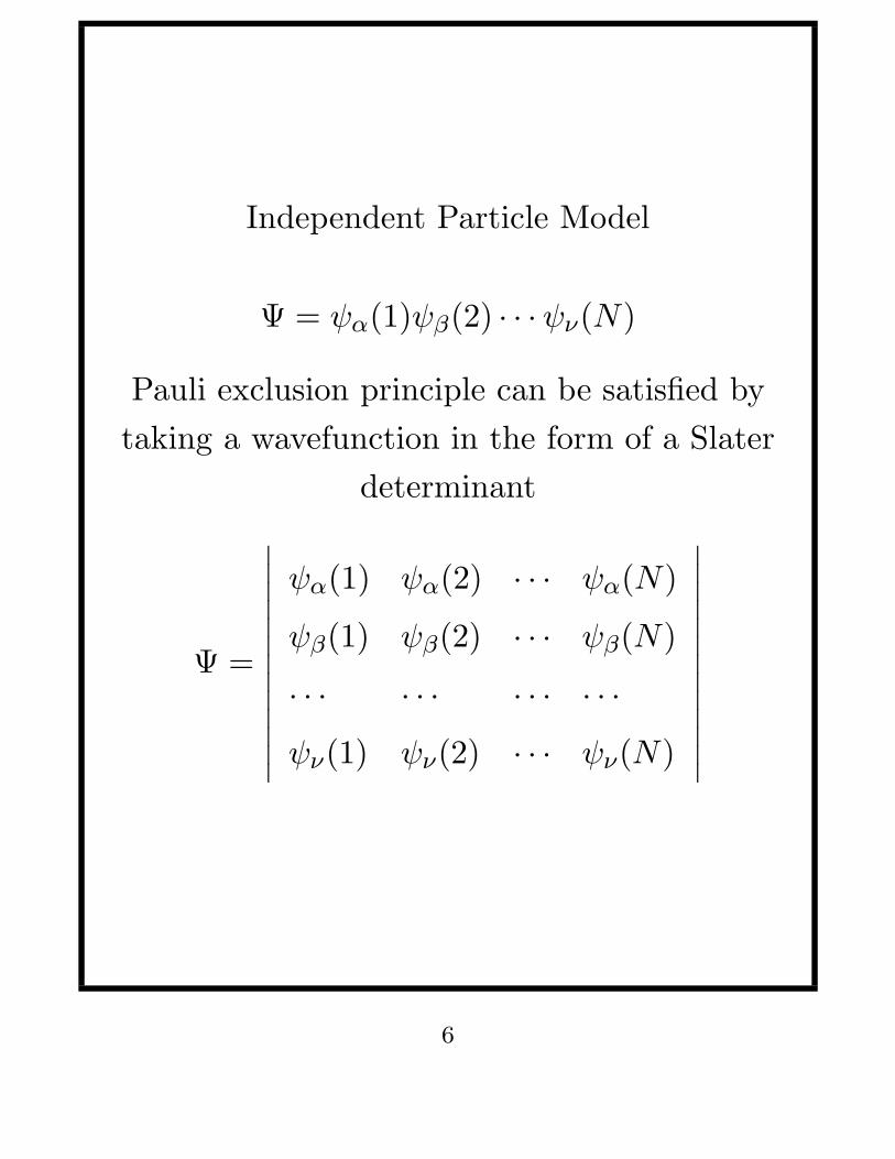
Independent Particle Model

Ψ = ψα(1)ψβ(2) · · ·ψν(N)

Pauli exclusion principle can be satisfied by

taking a wavefunction in the form of a Slater

determinant

Ψ =

∣

∣

∣

∣

∣

∣

∣

∣

∣

∣

∣

∣

∣

ψα(1) ψα(2) · · · ψα(N)

ψβ(1) ψβ(2) · · · ψβ(N)

· · · · · · · · · · · ·

ψν(1) ψν(2) · · · ψν(N)

∣

∣

∣

∣

∣

∣

∣

∣

∣

∣

∣

∣

∣

6

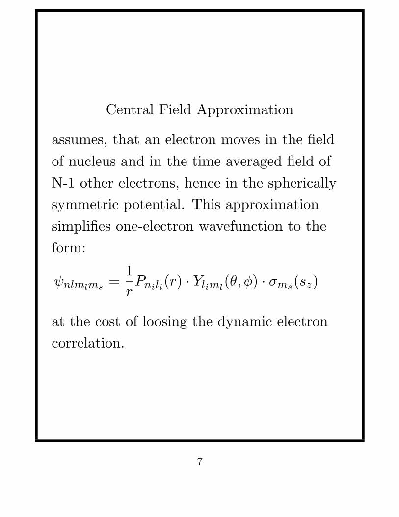
Central Field Approximation

assumes, that an electron moves in the field

of nucleus and in the time averaged field of

N-1 other electrons, hence in the spherically

symmetric potential. This approximation

simplifies one-electron wavefunction to the

form:

ψnlmlms=

1

rPnili(r) · Yliml

(θ, φ) · σms(sz)

at the cost of loosing the dynamic electron

correlation.

7

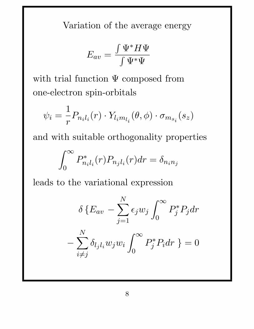
Variation of the average energy

Eav =

∫

Ψ∗HΨ∫

Ψ∗Ψ

with trial function Ψ composed from

one-electron spin-orbitals

ψi =1

rPnili(r) · Ylimli

(θ, φ) · σmsi(sz)

and with suitable orthogonality properties∫ ∞

0P ∗

nili(r)Pnj li(r)dr = δninj

leads to the variational expression

δ {Eav −N

∑

j=1

ǫjwj

∫ ∞

0P ∗

j Pjdr

−N

∑

i 6=j

δlj liwjwi

∫ ∞

0P ∗

j Pidr } = 0

8

Self-Consistent Field process

{ψi , i = 1, N}

Vi =

∫

ρ

rd3r =

N∑

j 6=i

e

∫

|ψj |2

rijd3r

(∇2

i

2−Z

ri+ Vi)ψi = ǫiψi , i = 1, N

{ψi , i = 1, N}

9

Hartree-Fock equation for the

spherically averaged atom

[−d2

dr2+li(li + 1)

r2−

2Z

r

+N

∑

j( 6=i)=1

wj

∫ ∞

0

2

r>P 2

j (r2)dr2

− (wi − 1)Ai(r) ]Pi(r)

= ǫiPi(r)

+N

∑

j( 6=i)=1

wj [δlilj ǫij +Bij(r)]Pj(r)

with the aid of the expansion

1

rij=

1

|~ri − ~rj |=

∞∑

k=0

rk<

rk+1>

Pk(cosθ)

10

Hartree-Fock local and non-local

potentials

Ai(r) =2li + 1

4li + 1

∑

k>0

li k li

0 0 0

2

·

∫ ∞

0

2rk<

rk+1>

P 2i (r2)dr2

and

Bij(r) =1

2

∑

k

li k li

0 0 0

2

·

∫ ∞

0

2rk<

rk+1>

Pj(r2)P2i (r2)dr2

11

Dirac-Coulomb Hamiltonian

H =∑

i

[

cαi · pi + c2(βi − 1) −Ze2

rj

]

+∑

i>j

e2

rij

Dirac-Hartree-Fock equations

cdQa

dr−cκ

rQa −

Z

rPa +

+∑

b,k

[

Ck(ab)Pa1

rYk(bb) +Dk(ab)Pb

1

rYk(ab)

]

= ǫaaPa +∑

b 6=a

qbǫabPb

−cdPa

dr−cκ

rPa − 2c2Qa −

Z

rQa +

+∑

b,k

[

Ck(ab)Qa1

rYk(bb) +Dk(ab)Qb

1

rYk(ab)

]

= ǫaaQa +∑

b 6=a

qbǫabQb

12

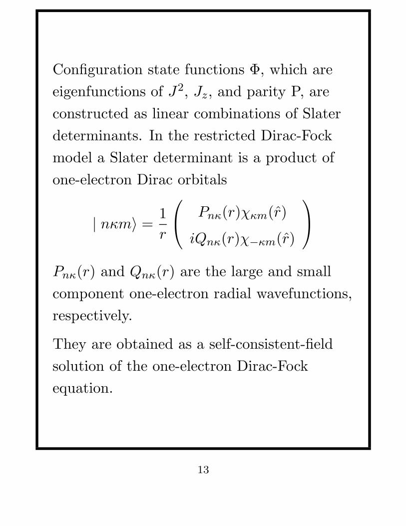
Configuration state functions Φ, which are

eigenfunctions of J2, Jz, and parity P, are

constructed as linear combinations of Slater

determinants. In the restricted Dirac-Fock

model a Slater determinant is a product of

one-electron Dirac orbitals

| nκm〉 =1

r

Pnκ(r)χκm(r)

iQnκ(r)χ−κm(r)

Pnκ(r) and Qnκ(r) are the large and small

component one-electron radial wavefunctions,

respectively.

They are obtained as a self-consistent-field

solution of the one-electron Dirac-Fock

equation.

13

One-electron quantum numbers

n principal quantum number

κ relativistic angular quantum number

κ = ±(j + 12) for l = j ± 1

2

m z-component

l orbital angular momentum of an electron

j total angular momentum of an electron

χ spinor spherical harmonic in the lsj

coupling scheme:

χκm(r) =

χκm(θ, ϕ, σ) =

σms〈lm−ms12ms | l

12jm〉Ylm−ms

(θ, ϕ)ξms(σ)

14

Methods for electron correlation

perturbation variational

Ψ =∞∑

n=0

(

HE0−H0

)nΨ0 Ψ =

∑

r

crΦr

linked-diagram Hylleraas

coupled-cluster Hartree-Fock

linked-cluster Dirac-Fock

15

Multi-Configuration Variational Wave

Function for Li 1s22s

1s22s single configuration

1s22s + 1s23s valence correlation

1s22s + 1s2s3s

1s22s + 1s2s3d core polarization

1s22s + 1s3s3d

1s22s + 2s3s3d core-core correlation

n1l1n2l2n3l3, ni = nL Layzer complex

n1l1n2l2n3l3, n ≤ nC Complete Active Space

16

no-pair Hamiltonian

Hnopair =N

∑

i=1

HD(ri) +∑

i<j

V(|~ri − ~rj |)

HD is the one electron Dirac operator

V represents the electron-electron interaction

of order α (one-photon exchange)

Vij in Coulomb gauge

Vij =1

rij

−αi · αj

rij

−αi · αj

rij[cos(

ωijrijc

) − 1]

− c2(αi · ~∇i)(αj · ~∇j)cos(

ωijrij

c) − 1

ω2ijrij

17

electron-electron interaction

a series expansion in powers of ωijrij/c << 1

Vij =1

rij(1)

−αi · αj

rij(2)

−αi · αj

rij[cos(

ωijrijc

) − 1] (3)

− c2(αi · ~∇i)(αj · ~∇j)cos(

ωijrij

c) − 1

ω2ijrij

(4)

rij = |~ri − ~rj | inter-electronic distance

ωij energy of the virtual photon

(1) Coulomb interaction

(2) Gaunt (magnetic) interaction

(3) and (4) retardation operator

18

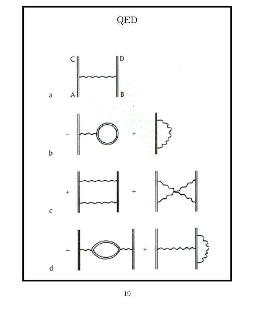
QED

19

MCHF and MCDF constraints

1. Theoretical model limits

• Schrodinger vs Dirac wave equation

– Breit (-Pauli) potential

• nuclear volume effects

– nuclear potential (point, spherical

ball, Fermi ball models)

– mass shift

– field shift

– extended nuclear multipole effects

(Bohr-Weisskopf effect)

• QED

2. Numerical limits

• grid

• orbital orthogonality

• variational instability

20

MCHF and MCDF applicability

• small, neutral or weekly ionised bound

systems

• oscillator strenghts

• autoionization rates

• hyperfine structures

• isotope shifts

21

Plans for the future

• non-orthogonal orbitals

• numerical grid, basis-set, splines

• general matrix element package

• P-, T-violation

• parallel processing (MPI)

• Fortran 90/95

22