Dimensional Analysis and Scalingjlogan1/PDFfiles/amch1.pdf · CHAPTER 1 Dimensional Analysis and...

CHAPTER 1

Dimensional Analysis and Scaling

1. Dimensional analysis

Exercise 1.1 The variables are t, r, ρ, e, P . We already know one dimensionlessquantity π1 = ρr5/et2. Try to find another in terms of P , which is a pressure,or force per unit area, that is, mass per length per time-squared. By inspection,π2 = t2P/r2ρ is another dimensionless quantity. Thus we have

f(ρr5/et2, t2P/r2ρ) = 0

Now we cannot isolate the r and t variables in one dimensionless expression; theymust occur in both. If we solve for the first dimensionless quantity we get

ρr5/et2 = F (t2P/r2ρ)

Then

r =

(

et2

ρ

)1/5

F (t2P/r2ρ)

Because the second dimensionless variable contains t and r in some unknown man-ner, we cannot conclude that r varies like t2/5. In this formulation, if one can arguethat the ambient pressure is small and can thus be neglected, then we can set P = 0and obtain the result

r =

(

et2

ρ

)1/5

F (0)

which does imply that r varies like t2/5.

Exercise 1.2 Here x = 0.5gt2; because g is an acceleration, we observe that π =x/gt2 is dimensionless. Clearly this is the only dimensionless combination. So thephysical law is π = 0.5. The law could not depend on mass because there are nodimensionless combinations of t, x, g that involve m.

2. The Buckingham Pi theorem

Exercise 2.1 Assume that f(v,Λ, g) = 0. If π is dimensionless

[π] = [vα1Λα2gα3 ]

= (LT−1)α1Lα2(LT−2)α3

1

2 1. DIMENSIONAL ANALYSIS AND SCALING

Thus we have the homogeneous system

α1 + α2 + α3 = 0, −α1 − 2α3 = 0

The rank of the coefficient matrix is one, so there is one dimensionless variable.Notice that (−2, 1, 1) is a solution to the system, and thus

π = Λg/v2

By the Pi theorem, F (π) = 0 or Λg/v2 = Const.

Exercise 2.2 Follow the idea in Example 2.3 on page 11. Pick length, time andmass as fundamental and write

x = λ1x, t = λ2t, m = λ3m

Then write v = λ1λ−12 v, and so on for the other variables. Show that

v − 2

9r2ρ g µ−1(1 − ρl/ρ) = λ1λ

−12 (v − 2

9r2ρgµ−1(1 − ρl/ρ))

So, by definition, the law is unit free.

Exercise 2.6 We have A = f(c, φ) = c2g(φ) since area is a length-squared. Nowapply the rule in the hint to the other two smaller, similar triangles to find theirareas as A1 = f(a, φ) = a2g(φ) and A2 = f(b, φ) = b2g(φ). Thus A = A1 + A2

implies c2 = a2 + b2.

Exercise 2.7 The period cannot depend only on the length and mass. Thereis no way that length and mass can be combined to yield a time dimension. Ifwe assume, however, that f(T, l,m, g) = 0, then there is only one dimensionless

variable, π = T√

g/l. (Again, mass will not appear). So, by the pi theorem,

T√

g/l =constant.

Exercise 2.9 Pick length L, time T , and mass M as fundamental dimensions.Then the dimension matrix has rank three and there are 5 − 3 = 2 dimensionlessvariables; they are given by π1 = γ and π2 = Rω

√ρl/

√P . Thus f(π1, π2) = 0

implies

ω = R−1√

P/ρlG(γ)

for some function G.

3. Scaling

Exercise 3.1 In (a) we have u = A sinωt and so u′ = ωA cosωt. Then M = Aand max |u′| = ωA. Then we have tc = 1/ω. In (b) we have u = Ae−λt and u′ =−λAe−λt. Then tc = max |u|/max |u′| = 1/λ. In part (c) we have u = Ate−λt andu′ = (1−λt)Ae−λt. The maximum of u occurs at t = 1/λ and is M = A/λe. To findthe maximum of u′ we calculate the second derivative to get u′′ = Aλ(λt− 2)e−λt.So the maximum derivative occurs at t = 2/λ or at an endpoint. It is easily checkedthat the maximum derivative occurs at t = 0 and has value max |u′| = A on thegiven interval. Therefore tc = (A/λe)/A = 1/λe.

3. SCALING 3

Exercise 3.2 Here u = 1 + exp(−t/ǫ) and u′ = −exp(−t/ǫ)/ǫ. Then tc =max |u|/max |u′| = 2/ǫ−1 = 2ǫ. The time scale is very small, indicating rapidchange in a small interval. But a graph shows that that this rapid decrease occursonly in a small interval near t = 0; in most of the interval the changes occur slowly.Thus two time scales are suggested, one near the origin and one out in the intervalwhere t is order one.

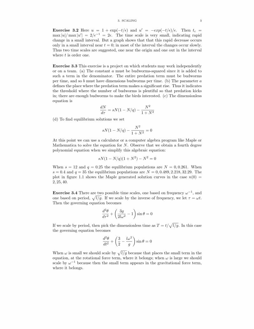
Exercise 3.3 This exercise is a project on which students may work independentlyor on a team. (a) The constant a must be budworms-squared since it is added tosuch a term in the denominator. The entire predation term must be budwormsper time, and so b must have dimensions budworms per time. (b) The parameter adefines the place where the predation term makes a significant rise. Thus it indicatesthe threshold where the number of budworms is plentiful so that predation kicksin; there are enough budworms to make the birds interested. (c) The dimensionlessequation is

dN

dτ= sN(1 −N/q) − N2

1 +N2

(d) To find equilibrium solutions we set

sN(1 −N/q) − N2

1 +N2= 0

At this point we can use a calculator or a computer algebra program like Maple orMathematica to solve the equation for N . Observe that we obtain a fourth degreepolynomial equation when we simplify this algebraic equation:

sN(1 −N/q)(1 +N2) −N2 = 0

When s = 12 and q = 0.25 the equilibrium populations are N = 0, 0.261. Whens = 0.4 and q = 35 the equilibrium populations are N = 0, 0.489, 2.218, 32.29. Theplot in figure 1.1 shows the Maple generated solution curves in the case n(0) =2, 25, 40.

Exercise 3.4 There are two possible time scales, one based on frequency ω−1, andone based on period,

√

l/g. If we scale by the inverse of frequency, we let τ = ωt.Then the governing equation becomes

d2θ

dτ2+

(

3g

2lω2− 1

)

sin θ = 0

If we scale by period, then pick the dimensionless time as T = t/√

l/g. In this casethe governing equation becomes

d2θ

dt2+

(

3

2− lω2

g

)

sin θ = 0

When ω is small we should scale by√

l/g because that places the small term in theequation, at the rotational force term, where it belongs; when ω is large we shouldscale by ω−1 because then the small term appears in the gravitational force term,where it belongs.


Figure 1. Budworm populations for problem 3.3.

Exercise 3.5 To solve P ′ = P (1 − P ), P (0) = α we separate variables andintegrate using partial fractions:

∫

1

P (1 − P )dP =

∫

dτ + c

or∫(

1

P+

1

1 − P

)

= τ + c

This gives

ln |P | − ln |p− 1| = τ + c

3. SCALING 5

orP

P − 1= Ceτ

The initial condition forces C = α/(α−1). This last expression can be manipulatedalgebraically to obtain equation (23) in the text.

Exercise 3.6 Introduce the following dimensionless variables:

m = m/M, x = x/R, t = t/T, v = v/V

where T and V are to be determined. In dimensionless variables the equations nowtake the form

m′ = −αTM

x′ = −V TRv

v′ =αβT

MV

1

m− Tg

V (1 − x)2

To ensure that the terms in the velocity and acceleration equations are the sameorder, with the gravitational term small, pick

V T

R=αβT

MV

which gives

V =√

αβR/M

as the velocity scale.

Exercise 3.7 The differential equation is

c′ = − q

V(ci − c) − kc2, c(0) = c0

Here k is a volume per mass per time. Choosing dimensionless quantities via

C = c/ci, τ = t/(V/q)

the model equation becomes

dC

dτ= −(1 − C) − bC2, C(0) = γ

where γ = c0/ci and b = kV ci/q. Solve this initial value problem using separationof variables or a computer algebra package.

Exercise 3.8 The quantity q is degrees per time, k is time−1, and θ is degrees (onecan only exponentiate a pure number). Introducing dimensionless variables

T = T/Tf , τ = t/(Tf/q)

we obtain the dimensionless model

dT

dτ= e−E/T − β(1 − T ), T (0) = α

where α = T0/Tf , E = θ/Tf , and β = kTf/q.


Exercise 3.9 Let h be the height measured above the ground. Then Newton’ssecond law gives

mh′′ = −mg − a(h′)2, h(0) = 0, h′(0) = V

Choose new dimensionless time and distance variables according to

τ = t/(V/g), y = h/(V 2/g)

Then the dimensionless model is

y′′ = −1 − α(y′)2, y(0) = 0, y′(0) = 1

where prime is a τ derivative and α = aV 2/mg.

Exercise 3.10 Scale time by√

l/g and angular displacement by θ0. Introducingthe dimensionless variables

τ = t/√

l/g, ψ = θ/θ0

gives the scaled model

d2ψ

dτ2+ θ−1

0 sin(θ0ψ) = 0, ψ(0) = 1, ψ′(0) = 0

CHAPTER 2

Perturbation Methods

1. Regular Perturbation

Exercise 1.1 Since the mass times the acceleration equals the force, we havemy′′ = −ky − a(y′)2. The initial conditions are y(0) = A, y′(0) = 0. Here, a isassumed to be small. The scale for y is clearly the amplitude A. For the timescale choose

√

m/k, which is the time scale when no damping is present. Letting

y = y/A, τ = t/√

m/k be new dimensionless variables, the model becomes

y′′ + ǫ(y′)2 + y = 0

where ǫ ≡ aA/m. The initial data is y(0) = 1, y′(0) = 0. Observe that the smallparameter is on the resistive force term, which is correct.

Exercise 1.2 The problem is

u′′ − u = ǫtu, u(0) = 1, u′(0) = −1

A two-term perturbation expansion is given by

y(t) = e−t +1

8ǫ(et − e−t(1 + 2x+ 2x2))

A six-term Taylor expansion is

y(t) = 1 − t+1

2t2 +

1 − ǫ

6x3 +

1 − 2ǫ

24x4 − 1 − 4ǫ

120x5

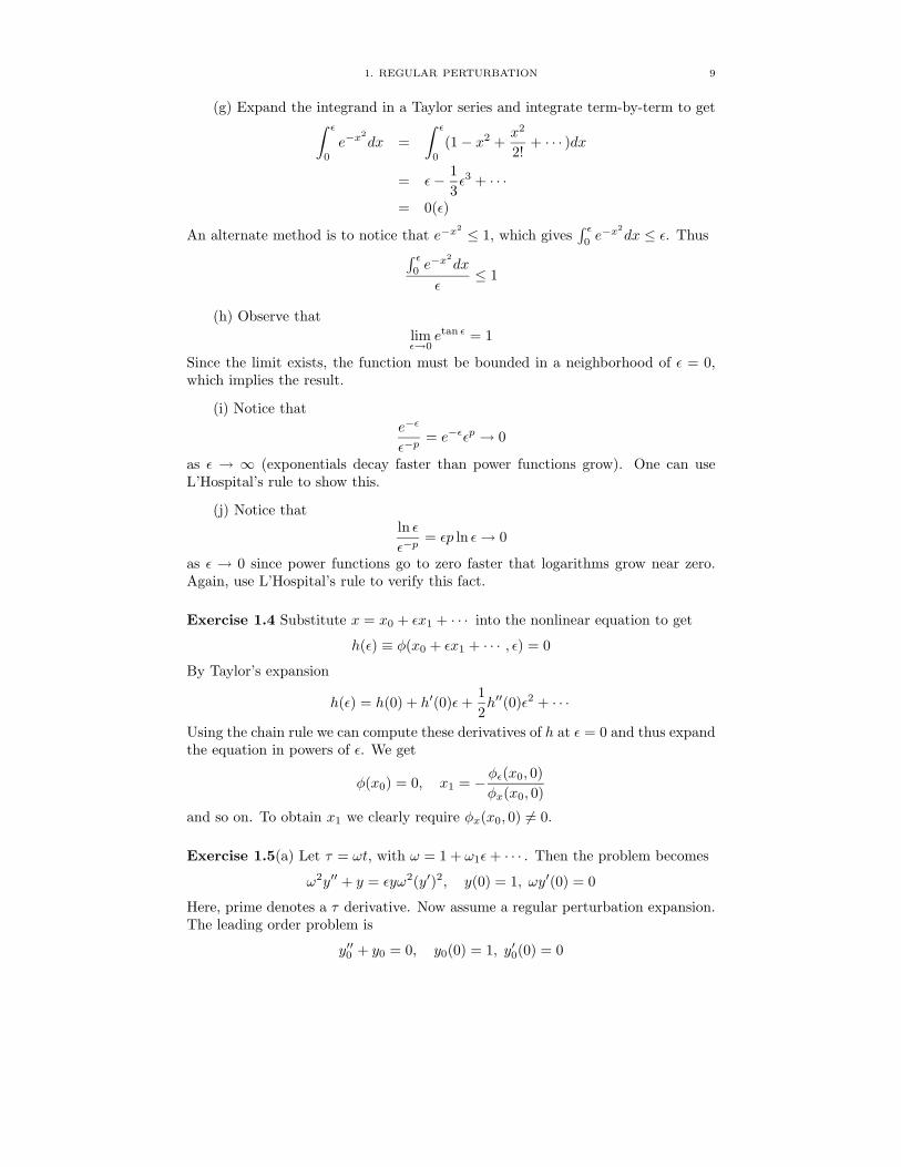
The plots in figure 1 show the superior performance of the two-term perturbationapproximation.

Exercise 1.3 (a) We have

t2 tanh t

t2= tanh t < 1

for large t. Thus t2 tanh t = 0(t2) as t→ ∞ .

(b) We have

limt→∞

e−t

1= 0

which proves the order relation.

(c) The order relation follows from the inequality√

ǫ(1 − ǫ)√ǫ

=√

1 − ǫ ≤ 1

for small, positive ǫ.

7

8 2. PERTURBATION METHODS

Figure 1. Graphs of exact solution, Taylor series approximation,and perturbation approximation in Exercise 1.2 when ǫ = 0.04.

(d) The idea is to expand cos ǫ in a power series to get√ǫ

1 − (1 − ǫ2/2 + ǫ4/4! − · · · )

=

√ǫ

ǫ2/2 − ǫ4/4! + · · · )

=1

2ǫ−3/2 1

1 − ǫ2/12 + · · ·But, using the geometric series,

1

1 − ǫ2/12 + · · · = 1 + 0(ǫ2)

which gives the result.

(e) We havet

t2=

1

t≤ 1

for large t. So the ratio is bounded, proving the assertion.

(f) By Taylor’s expansion

eǫ − 1 = 1 + ǫ+ 0(ǫ2) − 1 = 0(ǫ)

1. REGULAR PERTURBATION 9

(g) Expand the integrand in a Taylor series and integrate term-by-term to get∫ ǫ

0

e−x2

dx =

∫ ǫ

0

(1 − x2 +x2

2!+ · · · )dx

= ǫ− 1

3ǫ3 + · · ·

= 0(ǫ)

An alternate method is to notice that e−x2 ≤ 1, which gives∫ ǫ

0e−x2

dx ≤ ǫ. Thus∫ ǫ

0e−x2

dx

ǫ≤ 1

(h) Observe that

limǫ→0

etan ǫ = 1

Since the limit exists, the function must be bounded in a neighborhood of ǫ = 0,which implies the result.

(i) Notice that

e−ǫ

ǫ−p= e−ǫǫp → 0

as ǫ → ∞ (exponentials decay faster than power functions grow). One can useL’Hospital’s rule to show this.

(j) Notice thatln ǫ

ǫ−p= ǫp ln ǫ→ 0

as ǫ → 0 since power functions go to zero faster that logarithms grow near zero.Again, use L’Hospital’s rule to verify this fact.

Exercise 1.4 Substitute x = x0 + ǫx1 + · · · into the nonlinear equation to get

h(ǫ) ≡ φ(x0 + ǫx1 + · · · , ǫ) = 0

By Taylor’s expansion

h(ǫ) = h(0) + h′(0)ǫ+1

2h′′(0)ǫ2 + · · ·

Using the chain rule we can compute these derivatives of h at ǫ = 0 and thus expandthe equation in powers of ǫ. We get

φ(x0) = 0, x1 = − φǫ(x0, 0)

φx(x0, 0)

and so on. To obtain x1 we clearly require φx(x0, 0) 6= 0.

Exercise 1.5(a) Let τ = ωt, with ω = 1 + ω1ǫ+ · · · . Then the problem becomes

ω2y′′ + y = ǫyω2(y′)2, y(0) = 1, ωy′(0) = 0

Here, prime denotes a τ derivative. Now assume a regular perturbation expansion.The leading order problem is

y′′0 + y0 = 0, y0(0) = 1, y′0(0) = 0


which has solution

y0(τ) = cos τ

The next order problem is

y′′1 + y1 = −2ω1y′′0 + y0(y0)

2, y1(0) = 0, y′1(0) = 0

The equation simplifies to

y′′1 + y1 = (1

4+ 2ω1) cos τ − 1

4cos 3τ

To eliminate the secular term take ω1 = −1/8. Then, to leading order,

y0(t) = cos

((

1 − 1

8ǫ

)

t

)

Exercise 1.5(b) Let τ = ωt, with ω = 3 + ω1ǫ+ · · · . Then the problem becomes

ω2y′′ + 9y = 3ǫy3, y(0) = 0, ωy′(0) = 1

Here, prime denotes a τ derivative. Now assume a regular perturbation expansion.The leading order problem is

y′′0 + y0 = 0, y0(0) = 0, y′0(0) =1

3

which has solution

y0(τ) =1

3sin τ

The next order problem is

9y′′1 + 9y1 = 3y20 − 6ω1y

′′0 , y1(0) = 0, y′1(0) = −1

9

The equation simplifies to

y′′1 + y1 =1

9

(

1

12+ 2ω1

)

sin τ − 1

9 · 36sin 3τ

To eliminate the secular term take ω1 = −1/24. Then, to leading order,

y0(t) =1

3sin

((

3 − 1

24ǫ

)

t

)

Exercise 1.6 The equation with ǫ can be handled with a perturbation series in ǫ.After determining the coefficients, one can substitute ǫ = 0.001.

Exercise 1.7 If we ignor 0.01x in the first equation then y = 0.1. Then, fromthe second equation x = 0.9. Checking these values by substituting back into thefirst equation gives 0.01(0.9) + 0.1 = 0.109, so the approximation appears to begood. But the exact solution is x = 190, y = 1. So the approximation is in factterrible. What went wrong? Since x = −90 the first term in the first equationis 0.01x = −0.9, which is not small compared to the two other terms in the firstequation. Thus the first term cannot be neglected.

1. REGULAR PERTURBATION 11

Exercise 1.10 The three-term approximation is given by

ya(t) = t+t4

12ǫ+

t7

504ǫ2

The error is

E(t, ǫ) = y′′a − ǫtya = −ǫ3 t8

504

Clearly the approximation is not uniform on t ≥ 0.

Exercise 1.11 The leading order solution is

y0(t) =√t(1 − ln t)

Substituting into the ODE gives

Ly0 = − ǫ

2(1 + ln t)t3/2

We find

|Ly0| ≤ 0.0448

Thus one would expect y0 to be a good approximation on 0 ≤ t ≤ e.

Exercise 1.12 Substitute the series u = u0+u1ǫ+ · · · into the differential equationand initial conditions:

u′0 + u′1ǫ+ · · · + u0 + u1ǫ+ · · · =1

1 + u0ǫ+ · · ·= 1 − u0ǫ+ 0(ǫ2)

To get the last step we used the geometric series expansion. Now collecting thecoefficient of ǫ0 we get the leading order problem

u′0 + u0 = 1, u0(0) = 0

Collecting the coefficients of ǫ we get

u′1 + u1 = −u0, u1(0) = 0

The solution to the leading order problem (a linear equation) is

u0 = 1 − e−t

The the next order problem becomes

u′1 + u1 = e−t − 1, u1(0) = 0

This linear equation has solution

u1 = (t+ 1)e−t − 1

Therefore, a two-term approximation is

u(t) = 1 − e−t + ǫ((t+ 1)e−t − 1) + · · ·


2. Singular Perturbation

Exercise 2.1

(a) Consider the equation

ǫx4 + ǫx3 − x2 + 2x− 1 = 0

If x = O(1) then x2 − 2x + 1 ∼ 0 which means x ∼ 1, 1, a double root nearone. To find the remaining roots assume a dominant balance ǫx4 ∼ x2 with theremaining terms small. Then x = O(1/

√ǫ). This is a consistent balance because

ǫx4, x2 = O(1/ǫ) and the remaining three terms are are order one and small incomparison. So the dominant balance is

ǫx4 − x2 ∼ 0

which gives x ∼ ±1/√ǫ. So the leading order roots are

1, 1,±1/√ǫ

(b) The equation

ǫx3 + x− 2 = 0

has an order one root x ∼ 2. The consistent dominant balance is ǫx3 ∼ x whichgives x = O(1/

√ǫ). In this case we have ǫx3 + x ∼ 0, which gives the two other

leading order roots as

x ∼ ± i√ǫ

To find a higher order approximation for the root near x = 2 substitute x =2 + x1ǫ+ · · · into the equation and collect coefficients of ǫ to get x1 = −8. Thus

x = 2 − 8ǫ+ · · ·Since the other two roots are are order O(1/

√ǫ), let us choose a new order one

variable y given by

y = x/(1/√ǫ)

So, we are rescaling. Then the equation becomes

y3 + y − 2√ǫ = 0

and the small term appears where it should in the equation. Now assume y =y0 + y1

√ǫ + · · · , substitute into the equation, and collect coefficients to get at

leading order

y30 + y0 = 0

which gives y0 = ±i. At order O(√ǫ) we get the equation

3y20y1 + y1 − 2 = 0

Thus y1 = −1 and we have the expansions

y = ±i−√ǫ+ · · ·

In terms of x,

x = ± i√ǫ− 1 + · · ·

2. SINGULAR PERTURBATION 13

(c) The equation

ǫ2x6 − ǫx4 − x3 + 8 = 0

has three order one roots as solutions of −x3 + 8 = 0, or

x ∼ 2, −1 ±√

3i

To find the other roots, the dominant balance is ǫ2x6 − x3 ∼ 0, which gives

x ∼ 1

ǫ2/3e2πi/3,

1

ǫ2/3e−2πi/3

(d) The equation

ǫx5 + x3 − 1 = 0

has three order one roots (the cube roots of one) given by

x ∼ 1, −1

2±√

3i

The dominant balance for the remaining roots is between the first two terms whichgives

x ∼ ± i√ǫ


ǫy′′ + y′ + y = 0, y(0) = 0, y(1) = 0

When ǫ = 0 we get y′ + y = 0 which has solution y = ce−t. This cannot satisfyboth boundary conditions so regular perturbation fails.

The characteristic equation is ǫm2 + m + 1 = 0 which has two real, negativeroots given by

m1 =1

2ǫ(−1 +

√1 − 4ǫ) = −1 +O(ǫ)

m2 =1

2ǫ(−1 −

√1 − 4ǫ) = −1

ǫ+O(1)

Here we have used the binomial expansion√

1 + x = 1 + x/2 + O(x2) for small x.Note that one of the roots is order one, and one of the roots is large. So the generalsolution is

y(t) = c1em1t + c2e

m2t

Applying the boundary conditions gives the exact solution

y(t) =em1t − em2t

em1 − em2

Sketches of this solution show a boundary layer near t = 0 where there is a rapidincrease in y(t). Observe that em1 >> em2 . If t = O(1) then

em1t ∼ e−t, em2t ∼ 0

and thus

y(t) ∼ em1t

em1∼ e1−t


which is an outer approximation. If t = O(ǫ), then

y(t) ∼ e(−1+O(ǫ))t − e(−1/ǫ+O(1))t

em1

∼ eO(ǫ) − eO(ǫ)e−t/ǫ

em1

∼ 1 − e−t/ǫ

e−1

This is an inner approximation near t = 0.

Exercise 2.3 Observe that the equation can be written as a quadratic in ǫ:

2ǫ2 + xǫ+ x3 = 0

Thus

ǫ =1

4(−x±

√

x2 − 8x3)

These two branches can be graphed on a calculator, and the graph shows that thereis just one negative value for x, near x = 0, in the case that ǫ is small and positive.Thus assume

x = x1ǫ+ x2ǫ2 + · · ·

Substituting into the given equation gives

x = −2ǫ+ 8ǫ2 + · · ·

3. Boundary Layer Analysis

Exercise 3.2d The problem is

ǫy′′ + (1 + t)y′ + y = 0, y(0) = 0, y(1) = 1

By Theorem 3.1 in the text, there is a boundary layer at zero. The outer solutionis y0 = 2/(t + 1). In the boundary layer set τ = t/ǫ and Y (τ) = y(t). Then theinner equation is

Y ′′ + ǫτ + Y ′ + ǫY = 0

To leading order we have Y ′′i + Y ′

i = 0 with Yi(0) = 0. So the inner approximationis

Yi(τ) = A(1 − e−τ )

Matching gives A = 2 and so the uniform approximation is

y(t) =2

t+ 1+ 2(1 − e−t/ǫ) − 2

Exercise 3.2e The problem is

ǫy′′ + t1/3y′ + y = 0, y(0) = 0, y(1) = e−3/2

There is a boundary layer near t = 0. The outer solution is

y0(t) = exp(−1.5t2/3)

In the inner region set τ = t/δ(ǫ). Then the dominant balance is between the firstand second terms and δ = ǫ3/4. So the inner approximation to leading order is

Y ′′i + τ1/3Y ′

i = 0

3. BOUNDARY LAYER ANALYSIS 15

Solving gives

Yi(τ) = c

∫ τ

0

exp(−0.75s4/3)ds

Pick an intermediate variable to be η = t/√ǫ. Then matching gives

c =

(∫ ∞

0

exp(−0.75s4/3)ds

)−1

Exercise 3.2g The problem is

ǫy′′ + 2y′ + ey = 0, y(0) = y(1) = 0

There is a layer at zero. The outer solution is

y0(t) = − lnt+ 1

2

In the boundary layer the first two terms dominate and δ(ǫ) = ǫ. The inner solutionis

Yi(τ) = A(1 − e−2τ )

Matching gives A = ln 2. The uniform approximation is

y(t) = ln 2(1 − e−2t/ǫ) − lnt+ 1

2− ln 2

Exercise 3.2h The problem is

ǫy′′ − (2 − t2)y = −1, y(−1) = y(1) = 1

Now there are two layers near t = −1 and t = 1. The outer solution, which is validin the interval (−1, 1), away from the layers is

y0(t) =1

2 − t2

In the layer near t = 1 set τ = (1 − t)/δ(ǫ). We find δ =√ǫ with inner equation,

to leading order, Y ′′i − Yi = 1. The inner solution is

Yi(τ) = 1 + ae−τ − (1 + a)eτ

In the layer near t = −1 set τ = (t− 1)/δ(ǫ). We find δ =√ǫ with inner equation,

to leading order, (Y ∗i )′′ − Y ∗

i = −1. The inner solution is

Y ∗i (τ) = 1 + be−τ − (1 + b)eτ

Matching gives a = b = 1 and the uniform approximation is

y(t) =1

2 − t2− e(t−1)/

√ǫ − e(t+1)/

√ǫ


ǫy′′ +1

ty′ + y = 0, y(0 + 1, y′(0) = 0

which is an initial value problem and appears to be singular. But, the outer solutionis

y0(t) = Ce−t2/2


and it is observed that it satisfies both initial conditions when C = 1. It alsosatisfies the ODE uniformly, i.e.,

ǫy′′0 +1

ty′0 + y0 = ǫ(t2 − 1)e−t2/2 = O(ǫ)

Thus it provides a uniform approximation and the problem does not have a layer.It is instructive to try to put a layer at t = 0; one finds that no scaling is possible.

Exercise 3.7a By Theorem 3.1 the problem

ǫy′′ + (1 + t2)y′ − t3y = 0, y(0) = y(1) = 1

has a layer of order δ = ǫ at t = 0. The outer solution is

y0(t) =

√

2

1 + t2exp(

t2 − 1

2)

The inner solution is

Yi(τ) = A+ (1 −A)e−τ

Matching gives A =√

2/e.

Exercise 3.7b By Theorem 3.1 the problem

ǫy′′ + (cosh t)y −−y = 0, y(0) = y(1) = 1

has a layer of width δ = ǫ near t = 0. The outer solution is

y0(t) = exp(2 arctan et − 2 arctan e)

In the layer use the expansion

cosh z = 1 +1

2z2 + · · ·

The inner approximation is

Yi(τ) = 1 −A+Ae−τ

Matching gives A = 1 − exp(π/2 − 2 arctan e).

Exercise 3.7c The problem

ǫy′′ +2ǫ

ty′ − y = 0, y(0) = 0, y′(1) = 1

If we assume a layer at t = 1 the outer solution is y0(t) = 0. In the inner regionnear t = 1 the dominant balance is between the first and last terms and the widthof the layer is δ =

√ǫ. The inner variable is τ = (1 − t)/δ. The inner solution is

Yi(τ) = (√ǫ+ b)e−τ + beτ

We must set b = 0 to stay bounded. So the uniform solution is

y(t) =√ǫe(t−1)/

√ǫ

Exercise 3.7d In this problem we have an outer solution y0(t) = 0 which satisfiesboth boundary conditions exactly. So we have an exact solution y ≡ 0.

Exercise 3.7e The problem is

ǫy′′ +1

t+ 1y′ + ǫy = 0, y(0) = 0, y(1) = 1

4. TWO APPLICATIONS 17

The outer approximation is y0(t) =const, so there are several possibilities. Theidea that works is to assume a layer at t = 0 of width δ = ǫ which gives the innerapproximation

Y ′′i (τ) = a(1 − e−τ )

Matching gives a = 1.

4. Two Applications

Exercise 4.1 The equation my′′ + ay′ + by = 0 has characteristic roots

λ± = − a

2m± 1

2m

√

a2 − 4mk

Because m is small, the roots are real. The general solution is

y(t) = c1eλ−t + c2e

λ+t

Applying the initial conditions y(0) = 0, my′(0) = I, we get the exact solution

y(t) =I

m√a2 − 4mk

(

eλ+t − eλt)

Now, if m is small, then λ− ≈ −a/m and λ+ ≈ 0. Thus, for small m, the exactsolution is approximately

y(t) ≈ I

a(1 − e−at/m)

which agrees with the approximate solution in equation (14) in the text.

Exercise 4.2 If we make the change of variables

t = t/√

m/k, y = y/(I/a)

then we obtain the dimensionless initial value problem

ǫy′′ + y′ + ǫy = 0, y(0) = 0, y′(0) = ǫ−1

where

ǫ =√km/a << 1

Then, to leading order (setting ǫ = 0 in the differential equation) we have y′(t) = 0,or y(t) = const. = 0. So the outer approximation is zero, which is valid after a longtime.

Exercise 4.3 (a) In this case the system is

x′ = y − ǫ sinx, ǫy′ = x2y + ǫy3

with initial conditions x(0) = k, y(0) = 0. Setting ǫ = 0 we get the outer equations

x′0 = y0, 0 = x20y0

Here we can choose y0 = 0 and x0 = k and the initial conditions are met. So thisproblem does not have an initial layer. It is a regular perturbation problem withleading order solution

x0(t) = k, y0(t) = 0

It is instructive for the student to assume a layer near t = 0 and carry out theanalysis to find that the inner approximation agrees with the outer approximation.


(b) The problem is

u′ = v, ǫv′ = u2 − v, u(0) = 1, v(0) = 0

Assume a boundary layer near t = 0. Then the outer problem is

u′0 = v0, v0 = −u20

Then

u′0 = −u20

which has solution (separate variables)

u0(t) =1

t+ c, v0(t) =

−1

(t+ c)2

In the boundary layer take η = t/ǫ. Then the inner problem is

U ′ = ǫV, V ′ = −U2 − V, U(0) = 1, V (0) = 0

Thus, setting ǫ = 0 and solving yields the inner approximation

U(η) = const. = 1, V (η) = e−η − 1

Matching gives

limt→0

u0(t) = limη→∞

U(η)

or 1/c = 1. Hence, c = 1. Then the uniform approximation is

u =1

t+ 1+ 1 − 1 =

1

t+ 1

and

v =−1

(t+ 1)2+ e−t/ǫ − 1 − (−1) =

−1

(t+ 1)2+ e−t/ǫ

5. The WKB Approximation

Exercise 5.1 Letting ǫ = 1/√λ we have

ǫ2y′′ − (1 + x2)2y = 0, y(0) = 0, y′(0) = 1

This is the nonoscillatory case. From equation (10) on p 88 of the text the WKBapproximation is, after applying the condition y(0) = 0

yWKB =c1

1 + x2

[

exp

(√λ

∫ x

0

(1 + ξ2)2dξ

)

− exp

(

−√λ

∫ x

0

(1 + ξ2)2dξ

)]

=2c1

1 + x2sinh

(√λ

∫ x

0

(1 + ξ2)2dξ

)

Applying the condition y′(0) = 1 gives c1 = 1/2.

Exercise 5.2 Letting ǫ = 1/√λ we have

y′′ + λ(x+ π)4y = 0, y(0) = y(π) = 0

This is the oscillatory case and Example 5.3 on page 89 applies. The large eigen-values are

λn =

(

nπ∫ π

0(x+ π)2dx

)

=9n2

49π4

5. THE WKB APPROXIMATION 19

The eigenfunctions are

C

x+ πsin

(

3n

7π2

∫ x

0

(ξ + π)2dξ

)

=C

x+ πsin

(

3n

7π2(x3

x+ πx2 + π2x)

)

Exercise 5.3 The solution is a straightforward substitution.

Exercise 5.4 This problem is solved exactly like Exercise 5.1.

Exercise 5.5 Make the change of variables t = ǫx. Then the differential equationbecomes

ǫ2d2y

dt2+ q(t)2y = 0

which is equation (11) on page 88. So the approximation is given by equation (12)on page 89 with x replaced by ǫx.

We can think of the equation y′′ + q(ǫx)2y = 0 as a harmonic oscillator wherethe frequency is q(ǫx), which is time-dependent. (Here, think of x as time). If ǫ issmall, it will take a large time x before there is significant changes in the frequency.Thinking of it differently, if q(x) is a given frequency, then the graph of q(ǫx) willbe stretched out; so the frequency will vary slowly.

Exercise 5.6 Here we apply formula (12) on page 89 with k(x) = e2x and ǫ = 1/√λ.

Then the WKB approximation is

yWKB =c1ex

sin

(√λ

2(e2x − 1)

)

+c2ex

cos

(√λ

2(e2x − 1)

)

Applying the condition y(0) = 0 gives c2 = 0. Then

yWKB =c1ex

sin

(√λ

2(e2x − 1)

)

Then y(1) = 0 gives

sin

(√λ

2(e− 1)

)

= 0

and this forces

λ =4π2

(e− 1)2

for large n.

Exercise 5.9

(a) We have mx′′ = F (x). We use prime to denote time derivatives. Mul-tiplying by x′ and noting that x′x′′ = 1

2 ((x′)2)′ gives m2 ((x′)2)′ = F (x)x′. But

V (x)′ = (dV/dx)x′ = −F (x)x′, and so it follows that m2 ((x′)2)′ − V (x)′ = 0.

Integrating then givesm

2(x′)2 − V (x) = E

where E is a constant of integration.


(b) Letting p = mx′ in the last equation and then solving for p gives

p = ±√

2m(E − V (x))

6. Asymptotic Expansion of integrals

Exercise 6.2 Making the substitution t = tan2 θ gives

I(λ) =

∫ π/2

0

e−λ tan2 θdθ =1

2

∫ ∞

0

e−λtdt

(1 + t)√t

Now Watson’s lemma (Theorem 6.1) applies. But we proceed directly by expanding1/(1 + t) in its Taylor series

1

1 + t= 1 − t+ t2 − · · ·

which gives

I(λ) =1

2

∫ ∞

0

e−λt

√t

(1 − t+ t2 − · · · )dt

Now let u = λt. This gives

I(λ) =1

2√λ

∫ ∞

0

e−u

(

1√u−

√u

λ+u3/2

λ2+ · · ·

)

Then, using the defintion of the gamma function,

I(λ) =1

2√λ

(Γ(1

2) − 1

λΓ(

3

2) +

1

λ2Γ(

5

2) + · · · )

Exercise 6.3 Assume that g has a maximum at b with g′(b) > 0. Then expand

g(t) = g(b) + g′(b)(t− b) + · · ·The integral becomes

I(λ) =

∫ b

a

f(t)eλg(t)dt

=

∫ b

a

f(t)eλ(g(b)+g′(b)(t−b)+··· )dt

≈ f(b)eλg(b)

∫ b

a

eλg′(b)(t−b)dt

Now make the substitution v = λg′(b)(t− b) to obtain

I(λ) ≈ f(b)eλg(b) 1

λg′(b)

∫ 0

λg′(b)(a−b)

evdv

or

I(λ) ≈ f(b)eλg(b)

λg′(b)

∫ 0

−∞evdv

or

I(λ) ≈ f(b)eλg(b)

λg′(b)

for large λ.

6. ASYMPTOTIC EXPANSION OF INTEGRALS 21

If the maximum of g occurs at t = a with g′(a) < 0, then it is the samecalculation. We expand g in its Taylor series about t = a and we obtain the samesolution except for a minus sign and the b in the last formula replaced by a.

Exercise 6.4 (a) We have, using a Taylor expansion,

I(λ) =

∫ ∞

0

e−λt ln(1 + t2)dt

=

∫ ∞

0

e−λt(t2 − t4

2+t6

3− · · · )dt

Now let u = λt and we get

I(λ) =1

λ

∫ ∞

0

e−u(u2

λ2− u4

2λ4+

u6

3λ6+ · · · )dt

Using the definition of the gamma function, we obtain

I(λ) =1

λ(2!

λ2− 4!

2λ4+

6!

3λ6+ · · · )

(b) Let g(t) = 2t− t2. This function has its maximum at t = 1 where g′(1) = 0and g′′(1) = −2. Take f(t) =

√1 + t. Then

I(λ) =

∫ 1

0

√1 + teλ(2t−t2)dt ≈ 1

2f(1)eλg(1)

√

−2π

λg′′(1)

=

√

π

2λeλ

(c) Let g(t) = 1/(1 + t). This function has its maximum, with a negativederivative, at t = 1. Thus Exercise 6.3 holds. With f(t) =

√3 + t we have

I(λ) ≈ −f(1)eλg(1)

λg′(1)=

8

λeλ/2

Exercise 6.5 We have

Γ(x+ 1) =

∫ ∞

0

uxe−udu

Integrate by parts by letting r = ux and ds = e−udu. Then the integral becomes∫ ∞

0

uxe−udu = x

∫ ∞

0

e−uux−1du = xΓ(x)

Exercise 6.6 (b) Using the fact that e−t < 1 for t > 0, we have

|rn)λ)| = n!

∫ ∞

λ

e−t

tn+1dt

≤ n!

∫ ∞

λ

1

tn+1dt

= n!−1

ntn|∞λ = (n− 1)!

1

λn→ 0


as λ→ ∞.

(c) Observe that∫ ∞

λ

e−t

tn+1dt ≤ e−λ

λn+1

Then the ratio of rn to the last term of the expansion is

|rn(λ)|(n− 1)!e−λ/λn

≤ n

λ

This tends to zero as λ→ ∞. So the remainder is little oh of the last term, and sowe have an asymptotic series.

(d) Fix λ. The nth term of the series is does not converge to zero as n → ∞.Therefore the series does not converge.


I(λ) =

∫ ∞

0

1

t+ λ)2e−tdt

We integrate by parts letting

u =1

t+ λ)2, dv = e−t

We get

I(λ) =1

λ2− 2

∫ ∞

0

1

t+ λ)3e−tdt

Now integrate by parts again via

u =1

t+ λ)3, dv = e−t

Then

I(λ) =1

λ2− 2

λ3+ 6

∫ ∞

0

1

t+ λ)4e−tdt

Continuing in the same manner gives

I(λ) =1

λ2− 2!

λ3+

3!

λ2

+ · · · + n!

λn−1(−1)n+1 + (n+ 1)!

∫ ∞

0

1

t+ λ)n+2e−tdt

CHAPTER 3

Calculus of Variations

1. Variational Problems

Exercise 1.1 The functional is

J(y) =

∫ 1

0

(y′ sinπy − (y + t)2)dt

First note that if y(t) = −t then J(y) = 2/π. Now we have to show that J(y) < 2/πfor any other y. To this end,

J(y) =

∫ 1

0

(y′ sinπy − (y + t)2)dt

≤∫ 1

0

y′ sinπydt

= − 1

π

∫ 1

0

(cosπy)′dt

= − 1

π(cosπy(1) − cosπy(0)) ≤ 2

π

Exercise 1.2 Hint: substitute

y(x) = x+ c1x(1 − x) + c2x2(1 − x)

into the functional J(y) to obtain a function F = F (c1, c2) of the two variablesc1 and c2. Then apply ordinary calculus techniques to F to find the values thatminimize F , and hence J . That is, set ∇F = 0 and solve for c1 and c2.

2. Necessary Conditions for Extrema

Exercise 2.1 (a) The set of polynomials of degree ≤ 2 is a linear space. (b) Theset of continuous functions on [0, 1] satisfying f(0) = 0 is a linear space. (c) The setof continuous functions on [0, 1] satisfying f(0) = 1 is not a linear space because,for example, the sum of two such functions is not in the set.

Exercise 2.2 We prove that

||y||1 =

∫ b

a

|y(x)|dx

23

24 3. CALCULUS OF VARIATIONS

is a norm on the set of continuous functions on the interval [a, b]. First

||αy||1 =

∫ b

a

|αy(x)|dx = |α|∫ b

a

|y(x)|dx = |α| ||y||1

Next, if ||y||1 = 0 iff∫ b

a|y(x)|dx = 0 iff y(x) = 0. Finally, the triangle inequality if

proved by

||y + v||1 =

∫ b

a

|y(x) + v(x)|dx ≤∫ b

a

(|y(x)| + |v(x)|)dx

=

∫ b

a

|y(x)|dx+

∫ b

a

|v(x)|dx = ||y||1 + ||v||1

The proof that the maximum norm is, in fact, a norm, follows in the samemanner. To prove the triangle inequality use the fact that the maximum of a sumis less than or equal to the sum of the maximums.

Exercise 2.3 Let y1 = 0 and y2 = 0.01 sin 1000x. Then

||y1 − y2||s = max |0.01 sin 1000x| = 0.01

and

||y1 − y2||w = max |0.01 sin 1000x| + max |(0.01)(1000) cos 1000x| = 10.01


δJ(y0, αh) = limǫ→0

J(y0 + ǫαh) − J(w)

ǫ

= limǫ→0

αJ(y0 + ǫαh) − J(w)

ǫα

= limη→0

αJ(y0 + ηh) − J(w)

η

= αδJ(y0, h)

Exercise 2.5 (a) not linear; (b) not linear; (c) not linear; (d) not linear; (e) linear;(f) not linear.

Exercise 2.6 An alternate characterization of continuity of a functional that isoften easier to work with is: a functional J on a normed linear space with norm|| · || is continuous at y if for any sequence of functions yn with ||yn − y|| → 0 wehave J(yn) → J(y) as n→ 0.

(a) Now let ||yn − y||w → 0. Then ||yn − y||s → 0 (because ||v||s ≤ ||v||w). Byassumption J is continuous at y in the strong norm, and therefore J(yn) → J(y).So J is continuous in the weak norm.

(b) Consider the arclength functional J(y) =∫ b

a

√

1 + (y′)2dx. If two functionsare close in the strong norm, i.e., if the maximum of their difference is small, thenit is not necessarily true that their arclengths are close. For example, one mayoscillate rapidly while the other does not. Take y = 0 and y = n−1 sinnx for largen. These two functions are close in the strong norm, but not the weak norm.

2. NECESSARY CONDITIONS FOR EXTREMA 25

Exercise 2.7 Let yn → y in the strong norm. Then

|J(yn) − J(y)| ≤∫ b

a

||yn + y||s ||yn − y||sdx = (b− a)||yn + y||s ||yn − y||s

But ||yn + y||s ≤ M for some constant M since the sequence converges. Thus|J(yn) − J(y)| → 0.

Exercise 2.8

(a) δJ(y, h) =∫ b

a(hy′ + yh′)dx.

(b) δJ(y, h) =∫ b

a(2h′y′ + 2h)dx.

(c) δJ(y, h) = ey(a)h(a).(d) See Exercise 3.6.

(e) δJ(y, h) =∫ b

ah(x) sinx dx.

(f) δJ(y, h) =∫ b

a2y′h′ dx+G′(y(b))h(b).

Exercise 2.9 Let yn → y. Then J(yn) = J(yn − y) + J(y) → J(y) becauseJ(yn − y) → 0 (since yn − y → 0 and J is continuous at zero by assumption).


J(y + ǫh) =

∫ b

a

(

x(y′ + ǫh′)2 + (y + ǫh) sin(y′ + ǫh′)2)

dx

We must take the second derivative of this function of ǫ with respect to ǫ and thenset ǫ = 0. We obtain

δ2J =

∫ b

a

(2x(h′)2 − y(h′)2 sin y′ + 2hh′ cos y′)dx

Exercise 2.11 Here the functional is

J(y) =

∫ 1

0

(x2 − y2 + (y′)2)dx

Then

δJ(y, h) =

∫ 1

0

(−2yh+ 2y′h′)dx

Thus

δJ(x, x2) =3

2and

∆J = J(y + ǫh) − J(y) = J(x+ ǫx2) − J(x) = etc.

Exercise 2.13 In this case

J(y) =

∫ 2π

0

(y′)2dx

Then

J(y + ǫh) =

∫ 2π

0

(1 + ǫ cosx)2dx = 2π + ǫ2∫ 2π

0

cos2 xdx


Thend

dǫJ(y + ǫh) = 2ǫ

∫ 2π

0

cos2 xdx

and sod

dǫJ(y + ǫh) |ǫ=0= 0

Thus, by definition, J is stationary at y = x in the direction h = sinx. The familyof curves y + ǫh is shown in the figure.

Exercise 2.14 Here

J(y) =

∫ 1

0

(3y2 + x)dx+ y(0)2

Then

δJ(y, h) =

∫ 1

0

6yh dx+ 2y(0)h(0)

Substituting y = x and h = x+ 1 gives δJ = 5.

3. The Simplest Problem

Exercise 3.1 (a) The Euler equation reduces to an identity (0 = 0), and henceevery C2 function that satisfies the boundary conditions is an extremal. (b) TheEuler equation reduces to an identity (0 = 0), and hence every C2 function thatsatisfies the boundary conditions is an extremal. (c) The Euler equation reduces toy = 0, which does not satisfy the boundary conditions; so there are no extremals.

Exercise 3.2 (a) The Euler equation is

Ly − d

dxLy′ =

d

dx(2y′/x3) = 0

Thus

y(x) = Ax4 +B

(b) The Euler equation is

y′′ − y = ex

The general solution is

y(x) = Aex +Be−x +x

2ex

Exercise 3.3 The Euler equation is

Ly − d

dxLy′ = fy

√

1 + (y′)2 − d

dx

fy′√

1 + (y′)2= 0

Taking the total derivative and then multiplying by√

1 + (y′)2 gives

fy − y′fx − fy′′ +f(y′)2y′′

1 + (y′)2= 0

This reduces to

fy − y′fx − fy′′

1 + (y′)2= 0

3. THE SIMPLEST PROBLEM 27


− d

dxLy′ = 0

ory′

x√

1 + (y′)2= c

Solving for y′ (take the positive square root since, by the boundary conditons, wewant y′ > 0), separating variables, and integrating yields

y(x) =

∫

√

c2x2

1 − c2x2dx+ k

Then make the substitution u = 1 − c2x2 to perform the integration. We obtain

y(x) =1

c

√

1 − c2x2 + k

Applying the boundary conditions to determine the constants finally leads to

y(x) = −√

5 − x2 + 2

which is an arc of a circle.

Exercise 3.6 Let h ∈ C2. Then

δJ(y, h) =

∫ b

a

∫ b

a

K(s, t)[y(s)h(t) + h(s)y(t)]dsdt

+2

∫ b

a

y(t)h(t)dt− 2

∫ b

a

h(t)f(t)dt

Now, using the symmetry of K and interchanging the order of integration allowsus to rewrite the first integral as

2

∫ b

a

∫ b

a

K(s, t)y(s)h(t)dsdt

Then

δJ(y, h) = 2

∫ b

a

(

∫ b

a

K(s, t)y(s)ds+ y(t) − f(t)

)

h(t)dt

Thus∫ b

a

K(s, t)y(s)ds+ y(t) − f(t) = 0

This is a Fredholm integral equation (see Chapter 5) for y.


−((1 + x)y′)′ = 0

or

y′ = c1/(1 + x)

Integrating again

y(x) = c1 ln(1 + x) + c2


If y(0) = 0, y(1) = 1 then we get

y(x) =ln(1 + x)

ln 2

If the boundary condition at x = 1 is changed to y′(1) = 0, then the extremal isy(x) ≡ 0.

Exercise 3.8 In each case we minimize the functional T (y) given in equation (11)in the text. For example, in (a) we have n = ky and so the Euler equation reducesto

ky√

1 + (y′)2= c

Solving for y′ and then separating variables gives

±dx =dy

√

C21y

2 − 1

This integrates to

±x+ c2 =1

c1cosh−1(c1y)

So y is a hyperbolic cosine.

Exercise 3.9 Observe that

Lt −d

dt(L− y′Ly′) = Lt −

dL

dt+ y′

dLy′

dt+ y′′Ly′

= Lt − Lt − Lyy′ − Ly′y′′ + y′

dLy′

dt+ y′′Ly′

= −y′(Ly − d

dtLy′)

Exercise 3.10 The minimal surface of revolution is found by minimizing

J(y) =

∫ b

a

2πy√

1 + (y′)2dx

Because the integrand does not depend explicitly on x, a first integral is

L− y′Ly′ = c

Upon expanding and simplifying, this equation leads to

dy

dx=√

k2y2 − 1

Now separate variables and integrate while using the fact that

d

ducosh−1 u =

1√u2 − 1

Exercise 3.11 The Euler equation becomes

x2y′′ + 2xy′ − y = 0

which is a Cauchy-Euler equation. Its solution is

y(x) = Ax(−1+√

5)/2 +Bx(−1−√

5)/2

4. GENERALIZATIONS 29

(recall that a Cauchy-Euler equation can be solved by trying power functions, y =xm for some m).

4. Generalizations

Exercise 4.1 By way of contradiction, assume f is strictly positive at some pointx = c. By continuity, f is positive in some open interval I = (c − ǫ, c + ǫ). Takeh(x) = (x − c + ǫ)5(c + ǫ − x)5 in I and zero otherwise. Having the fifth poweron these factors makes h four times continuously differentiable. This gives the

contradiction since∫ b

ah(x)f(x)dx > 0.

Exercise 4.2 (a) The Euler equations are

8y1 − y′′2 = 0, 2y2 − y′′1 = 0

Eliminating y2 gives

y′′′′1 − 16y1 = 0

The characteristic equation is m4−16 = 0, which has roots m = ±2,±2i. Thereforethe solution is

y1(x) = ae2x + be−2x + c cos 2x+ d sin 2x

where a, b, c, d are arbitrary constants. Then y2 = 0.5y′′1 , and the four constantsa, b, c, d can be computed from the boundary conditions.


y′′′′ = 0

and thus the extremals are

y(x) = a+ bx+ cx2 + dx3

The four constants a, b, c, d can be computed from the boundary conditions.

Exercise 4.3 The Euler equation for j(y) =∫

L(x, y, y′, y′′)dx is

Ly − (Ly′)′ + (Ly′′)′′ = 0

If Ly = 0 then clearly

Ly′ − (Ly′′)′ = const.

If Lx = 0, then expand all the derivatives and use the Euler equation to show

d

dx(L− y′(Ly′ − (Ly′′) − y′′Ly′′)) = 0

Exercise 4.4 (a) The Euler equation simplifies to y′′′′ = 0 and thus the extremalsare

y(x) = a+ bx+ cx2 + dx3

The four constants a, b, c, d can be computed from the boundary conditions.(b) The Euler equation simplifies to

y′′′′ + y = 0


The characteristic equation is m4 + 1 = 0, which has the four complex roots

m =1√2(1 + i),

1√2(1 − i),

1√2(−1 + i),

1√2(−1 − i)

Therefore the general solution is

y(x) = ex/√

2

(

a cosx√2

+ b sinx√2

)

+ e−x/√

2

(

c cosx√2

+ d sinx√2

)

Observe that a = b = 0 in order to meet the boundary conditions at x = +∞. Theboundary conditions at x = 0 determine c and d.


(x2ux)x + (y2uy)y = 0


utt − c2uxx = 0

which is the wave equation.


utt −m2u = ∆u

where ∆u = uxx + uyy + uzz is the Laplacian operator.


y′′′′ − 2y′′ + y = 0

This constant coefficient equation has characteristic equation m4−2m2+1 = 0 withroots m = ±1,±1. So, both 1 and −1 are double roots. Therefore the extremalsare

y(x) = aex + bxex + ce−x + dxe−x

Exercise 4.10 The two Euler equations (expanded out) are

Ly′y′y′′ + Ly′z′z′′ = 0

Lz′y′y′′ + Ly′z′z′′ = 0

It is given that the determinant of the coefficient matrix of this system is nonzero.Therefore the only solution is y′′ = z′′ = 0, which gives linear functions for y andz.


y′′ − y = 0

which gives

y(x) = aex + be−x

One boundary condition is y(0) = 1. The natural boundary condition is y′(1) = 0.These two conditions determine a and b.

4. GENERALIZATIONS 31

(b) The Euler equation reduces to y′′ − 1 = 0 which leads to

y(x) =1

2x2 + ax+ b

The natural boundary condition is y′(1) + y(1) + 1 = 0. This condition, with thegiven condition y(0) = 0.5 determines a and b.


x2y′′ + 2xy′ +1

4y = 0

which is a Cauchy-Euler equation. Assuming solutions of the form y = tm givesthe characteristic equation

m(m− 1) + 2m+1

4= 0

which has a real double root m = − 12 . Thus the general solution is

y(x) = a1√x

+ b1√x

lnx

The given boundary condition is y(1) = 1; the natural boundary condition at x = eis y′(e) = 0. One finds from these two conditions that a = b = 1.

Exercise 4.14 The first variation of the functional is

δJ(u, h) =

∫

R

E(x, y)dxdy +

∫

C

(−hLuydx+ hLux

dy)

where E is the Euler expression. Pick h such that h = 0 on C. Then E = 0 by thefundamental lemma. Thus

∫

C

(−hLuydx+ hLux

dy) = 0

for all h. But this last condition forces

−Luydx+ Lux

dy = 0

on C or

(Lux, Luy

) · n = 0

where n is the outward unit normal to C.

Exercise 4.15 Using Exercise 4.14 we find that the natural boundary condition isa∇u · n = 0 on the curve Bd R.

Exercise 4.16 The natural boundary condition is

Ly′(b, y(b), y′(b)) +G′(y(b)) = 0

Exercise 4.17 Using the last problem the natural boundary condition is y′(1) +y(1) = 0. The extremal is

y(x) = −1

2x+ 1

.


5. Hamiltonian Theory

Exercise 5.1 The Hamiltonian is

H(t, y, p) =p2

4r(t)− q(t)y2

Hamilton’s equations are

y′ =p

2r(t), p′ = 2q(t)y

Exercise 5.2 Here we have

J(y) =

∫

√

(t2 + y2)(1 + (y′)2)

We find

p = Ly′ =

√

t2 + y2y′√

1 + (y′)2

which yields

(y′)2 =p2

t2 + y2 − p2

The Hamiltonian simplifies, after some algebra, to

H(t, y, p) = −√

t2 + y2 − p2

Then Hamilton’s equations are

dy

dt=

p√

t2 + y2 − p2,

dp

dt=

y√

t2 + y2 − p2

Dividing the two equations givesdy

dp=p

yIntegrating yields

y2 − p2 = const

These are hyperbola in the yp phase plane.

Exercise 5.3 Hamilton’s equations for the pendulum are

θ′ =p

ml2, p′ = −mgl sin θ

Exercise 5.4 (a) The potential energy is the negative integral of the force, or

V (y) = −∫

(−ω2y + ay2)dy =1

2ω2y2 − 1

3ay3

The Lagrangian is L = 12m(y′)2−V (y). The Euler equation concides with Newton’s

second law:my′′ = −ω2y + ay2

(b) The momentum is p = Ly′ = my′, which gives y′ = p/m. The Hamiltonianis

H(y, p) =1

2(p/m)2 + V (y)

5. HAMILTONIAN THEORY 33

which is the kinetic plus the potential energy, or the total energy of the system.Yes, energy is conserved (L is independent of time).

(c) We have H = E for all time t, so at t = 0 we have

1

2(p(0)/m)2 + V (y(0)) =

ω2

10

If y(0) = 0 we can solve for p(0) to get the momentum at time zero; but this gives

y′(0) = ±√

ω2/5m

(d) and (e) The potential energy has a local maximum at y = ω2/a and is equalto

Vmax = V (ω2/a) =ω6

6a2

Note that V = 0 at y = 0, 3ω2/2a. If E < Vmax then we obtain oscillatory motion;if E > Vmax, then the motion is not oscillatory. Observe that the phase diagram(the solution curves in yp–space, or phase space), can be found by graphing

p = ±√

2m(E − V (y)

for various constants E.

Exercise 5.6 Here the force is F (t, y) = ket/y2. We can define a potential byV (t, y) = −

∫

F (t, y)dy = ket/y. The Lagrangian is

L(t, y, y′) =m

2(y′)2 − V (t, y)

The Euler equation ismy′′ − ket/y2 = 0

which is Newton’s second law of motion. The Hamiltonian is

H(t, y, p) =p2

2m+k

yet

which is the total energyy. Is energy conserved? We can compute dH/dt to find

dH

dt= ket/y 6= 0

So the energy is not constant.

Exercise 5.7 The kinetic energy is T = m(y′)2/2. The force is mg (with a plussign since positive distance is measured downward). Thus V (y) = −mgy. Thenthe Lagrangian is L = m(y′)2/2 +mgy.

Exercise 5.9 The Lagrangian does not depend explicitly on the independent vari-able x and therefore a first integral can be calculated from

L− y′Ly′ = C

Exercise 5.10 Pick r and θ as generalized coordinates. Then T = (m/2)((r′)2 +r2(θ′)2). There are two contributions to the potential energy, one due to gravityand the other due to the spring. We have

V (y) = mg(l − r cos θ) +k

2(l − r)2


Therefore the Lagrangian is

L(r, θ, r′, θ′) =m

2((r′)2 + r2(θ′)2) −mg(l − r cos θ) − k

2(l − r)2

The two equations of motion are

(r2θ′)′ + gr sin θ = 0, mr′′ −mr(θ′)2 −mg cos θ − k(l − r) = 0

Exercise 5.11 We have r′ = −α and so r(t) = −αt+ l. Then the kinetic energy is

T =m

2((r′)2 + r2(θ′)2) =

m

2(α2 + (l − αt)2(θ′)2)

and the potential energy is

V = mgh = mg(l − r cos θ) = mg(l − (l − αt) cos θ)

The Lagrangian is L = T − V . The Euler equation, or the equation of motion, is

g sin θ + (l − αt)θ′′ − 2αθ = 0

One can check that the Hamiltonian is not the same as the total energy; energy isnot conserved in this system. If fact, one can verify that

d

dt(T + V ) = −mgα cos θ 6= 0

Exercise 5.14 The Emden-Fowler equation is

y′′ +2

ty′ + y5 = 0

Multiply by the integrating factor t2 to write the equation in the form

(t2y′)′ + t2y5 = 0

Now we can identify this with the Euler equation:

Ly = −t2y5, Ly′ = t2y′

Integrate these two equations to find

L =1

2t2(y′)2 − 1

6t2y6 + φ(t)

Exercise 5.15 Multiply y′′ + ay′ + b = 0 by the integrating factor exp(at) to get

(eaty′)′ + beat = 0

Now identify the terms in this equation with the terms in the Euler equation as inExercise 5.14. Finally we arrive at a Lagrangian

L = eat(m

2(y′)2 − by

)

There are many Lagrangians, and we have chosen just one by selecting the arbitraryfunctions.

Exercise 5.16 Follow example 5.6 in the book with m,a, k and y replaced byL,R,C−1 and I, respectively.

6. ISOPERIMETRIC PROBLEMS 35

Exercise 5.17 For which Lagrangians is the Euler equation satisfied identically forevery y? The Euler equation is

Ly − Lty′ − Lyy′y′ − Ly′y′y′′ = 0

IF this equation holds for every function y then we can pick y so that the first threeterms vanish, and thus

Ly′y′ = 0

Hence Ly′ = φ(t, y), where φ is an arbitrary function. Hence,

L = φ(t, y)y′ + ψ(t, y)

where ψ is another arbitrary function.

6. Isoperimetric Problems

Exercise 6.1 Let L∗ = x2 + (y′)2 + λy2. Then the Euler equation for L∗ is

y′′ + λy = 0, y(0) = y(1) = 0

If λ ≥ 0 then this boundary value problem has only trivial solutions. If λ < 0, sayλ = −β2, then the problem has nontrivial solutions

yn(x) = Bn sinnπx, n = 1, 2, . . .

where the Bn are constants. Applying the constraint gives∫ 1

0

B2n sin2 nπx dx = 2

Thus Bn = ±2 for all n. So the extremals are

yn(x) = ±2 sinnπx, n = 1, 2, . . .

Exercise 6.2 The Euler equations become

L∗y1

− d

dxL∗

y1= 0, L∗

y2− d

dxL∗

y2= 0

where L∗ = L+ λG.

Exercise 6.3 Form the Lagrangian

L∗ = xy′ − yx′ + λ√

(x′)2 + (y′)2

Since the Lagrangian does not depend explicitly on t, a first integral is given by

L∗ − x′L∗x′ − y′L∗y′ = c

Exercise 6.4 The problem is to minimize

J(y) =

∫ 1

0

√

1 + (y′)2dx, y(0) = y(1) = 0

subject to the constraint∫ 1

0

y(x)dx = A


Form the Lagrangian

L∗ =√

1 + (y′)2 + λy

Since the Lagrangian does not depend explicitly on x, a first integral is given by

L∗ − y′L∗y′ = c

Expanding out this equation leads to

y′ =

√

1 − (λy − c)2

(λy − c)2

Separating variables and integrating, and then using the substitution u = 1− (λy−c)2, gives

− 1

2λ

∫

du√u

= x+ c1

Thus

(x+ c1)2 + (y − c/λ)2 =

1

λ2

which is a circle. Now the two boundary conditions and the constraint give threeequations for the constants c, c1, λ.


L∗ = p(y′)2 + qy2 + λry2

Then the Euler equation corresponding to L∗ is

Ly − (Ly′)′ = 2qy + 2rλy − 2(py′)′ = 0

or

(py′)′ − qy = rλy, y(a) = y(b) = 0

This is a Sturm-Liouville problem for y (see Chapter 4).

Exercise 6.6 Solve the constraint equation to obtain

z = g(t, y)

Substitute this into the functional to obtain

W (y) ≡∫ b

a

F (t, y, y′) ≡∫ b

a

L(t, y, g(t, y), y′, gt + gyy′)dt

Now form the Euler equation for F . We get

Fy − d

dtFy′ = 0

or, in terms of L,

Ly + Lzgy + Lz′(gty + gyyy′) − d

dt(Ly′ + Lz′gy) = 0

This simplifies to

Ly − d

dtLy′ + gy(Lz −

d

dtLz′ = 0

Also G(t, y, g(t, y)) = 0, and taking the partial with respect to y gives

Gy +Gzgy = 0


ThusLy − d

dtLy′

Gy=Lz − d

dtLz′

Gy

Now these two expressions must be equal to the same function of t, that is

Ly − d

dtLy′ = λ(t)Gy, Lz −

d

dtLz′ = λ(t)Gz


L∗ = (y′)2 + λy2

The Euler equation reduces to

y′′ − λy = 0, y(0) = y(π) = 0

This is similar to Exercise 6.1. The extremals are given by

yn(x) = ±√

2/π sinnx, n = 1, 2, 3, . . .


Figure 1. Exercise 1

Additional Exercises

1. (See the figure below) A drop of a viscous fluid with viscosity µ, measured inunits of grams/(sec cm), and density ρ is sitting on a flat plate, making contactarea A with the plate. The drop has volume V . The fluid drop is surrounded byan inviscid (viscosity zero) fluid of the same density ρ which is moving with speedU . Let τ be the time taken for the drop to move. (a) Use dimensional analysis todetermine a functional relation for τ in terms of a minimal number of parametercombinations. (b) Suppose it is known that τ is inversely proportional to µ. Doesthis additional information allow a more precise characterization of the functionalform for τ?

2. Consider the following differential equation for u = u(t), t > 0, where a is apositive real number:

du

dt= (1 − u)(u2 − a)

(a) find all the equilibrium solutions and (b) determine a condition on a that willguarantee that u = 1 is an attractor.

3. Consider the initial value problem

d2y

dt2+ 9y = 3ǫy3, y(0) = 0, y′(0) = 1

where 0 < ǫ << 1. Find the leading order perturbation approximation using thePoincare-Lindstedt method (make sure your approximation contains the adjustedfrequency).

4. Prove that3x2ǫ2

x2 + 1= O(ǫ2)

as ǫ→ 0, uniformly on x ≥ 0.


5. Find a two-term perturbation approximation on 0 ≤ x ≤ 1 for the solution y(x)of

y′ + y =1

1 + ǫ√y, y(0) = 0, 0 < ǫ << 1

.

6. Write down an order relation with big oh or little oh that expresses the fact thate−x decays faster than 1/x2 as x→ +∞, and then prove your assertion.

7. Consider the equation 0.0001x4 − 0.01x + 1 = 0. To leading order, determinethe roots. (Recall that

√i = ± 1√

2(1 + i)).

8. A functional J , defined on the set A of all y ∈ C2[0, 1] with y(0) = y(1) = 0, isdefined by

J(y) =

∫ 1

0

√

1 + (y′)2dx

Let h ∈ C2[0, 1] with h(0) = h(1) = 0. Compute δJ(y, h).

9. Find a one-term approximation for the large eigenvalues λ of the problem

y′′ + λ2e2xy = 0, 0 < x < 1, y(0) = y(1) = 1

10. Find a leading order approximation on 0 ≤ x ≤ 1 to the solution of the problem

ǫy′′ + 2y′ + y3 = 0, y(0) = 0, y(1) =1

2

11. Consider the initial value problem

ǫe−tu′′ + u′ = 1 − 2t, t > 0, u(0) = 1, ǫu′(0) = −1

where 0 < ǫ≪ 1 and u = u(t). Find a leading order approximation for the solution.

12. Find the extremal for the functional

J(y) =

∫ 1

0

(1 + x)(y′)2dx, y(0) = 0, y(1) = 1

13. Find a two-term approximation for all the real roots of the equation eǫx = x2−1where 0 < ǫ≪ 1.

14. Find the leading order behavior of the integral∫ 1

0e−λt3dt for large λ.

15. Consider the following functional defined over the set of C2 functions satisfyingy(0) = 1 and y(b) = 0:

J(y) =

∫ b

0

(G(y)(y′)2 −G(y)2)dx

where G is a given differentiable function.


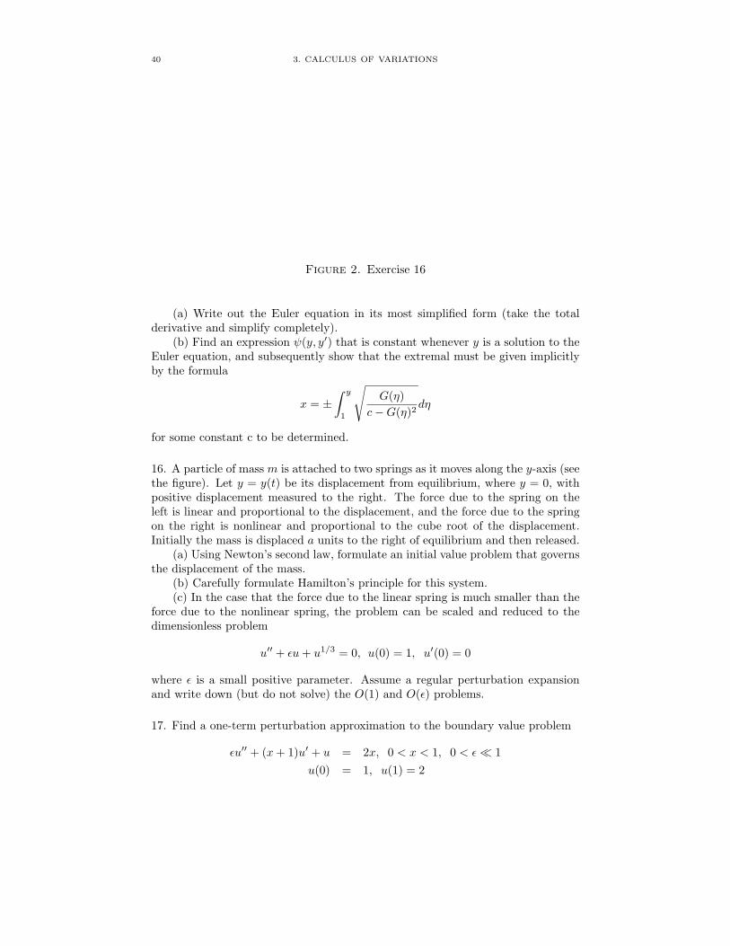
Figure 2. Exercise 16

(a) Write out the Euler equation in its most simplified form (take the totalderivative and simplify completely).

(b) Find an expression ψ(y, y′) that is constant whenever y is a solution to theEuler equation, and subsequently show that the extremal must be given implicitlyby the formula

x = ±∫ y

1

√

G(η)

c−G(η)2dη

for some constant c to be determined.

16. A particle of mass m is attached to two springs as it moves along the y-axis (seethe figure). Let y = y(t) be its displacement from equilibrium, where y = 0, withpositive displacement measured to the right. The force due to the spring on theleft is linear and proportional to the displacement, and the force due to the springon the right is nonlinear and proportional to the cube root of the displacement.Initially the mass is displaced a units to the right of equilibrium and then released.

(a) Using Newton’s second law, formulate an initial value problem that governsthe displacement of the mass.

(b) Carefully formulate Hamilton’s principle for this system.(c) In the case that the force due to the linear spring is much smaller than the

force due to the nonlinear spring, the problem can be scaled and reduced to thedimensionless problem

u′′ + ǫu+ u1/3 = 0, u(0) = 1, u′(0) = 0

where ǫ is a small positive parameter. Assume a regular perturbation expansionand write down (but do not solve) the O(1) and O(ǫ) problems.

17. Find a one-term perturbation approximation to the boundary value problem

ǫu′′ + (x+ 1)u′ + u = 2x, 0 < x < 1, 0 < ǫ≪ 1

u(0) = 1, u(1) = 2


18. Consider the functional defined by

J(u) =

∫ b

a

p(x)2(u′)2dx, u(a) = A, u(b) = B; p ∈ C[a, b], p > 0

Find an explicit formula for the extremal.

19. Find a three-term asymptotic approximation to the function

I(x) =

∫ x

0

e−s2

dx

as x→ 0.

20. Consider the problem

ǫu′′ + b(t)u′ + u = 0, 0 < t < T ; 0 < ǫ≪ 1

u(0) = 0, u′(0) = β/ǫ+ γ

where b is smooth and b(t) > 0, and T, β, γ > 0. Find a uniformly valid, leadingorder approximation to this problem.

Dimensional Analysis and Scalingjlogan1/PDFfiles/amch1.pdf · CHAPTER 1 Dimensional Analysis and...

Documents

Transcript of Dimensional Analysis and Scalingjlogan1/PDFfiles/amch1.pdf · CHAPTER 1 Dimensional Analysis and...