Dimension and Lyapunov exponents in conformal non ...im.ufrj.br/gelfert/T_Gelfert_Rams_1.pdf ·...
45
Dimension and Lyapunov exponents in conformal non-hyperbolic dynamics 1. Multifractal analysis of uniformly hyperbolic systems Katrin Gelfert (IM-UFRJ), Michal Rams (IMPAN) Będlewo, 2013 (Będlewo, 2013) Dimension and Lyapunov exponents 1 / 13
Transcript of Dimension and Lyapunov exponents in conformal non ...im.ufrj.br/gelfert/T_Gelfert_Rams_1.pdf ·...
Dimension and Lyapunov exponentsin conformal non-hyperbolic dynamics
1. Multifractal analysis of uniformly hyperbolic systems
Katrin Gelfert (IM-UFRJ), Michał Rams (IMPAN)
Będlewo, 2013
(Będlewo, 2013) Dimension and Lyapunov exponents 1 / 13
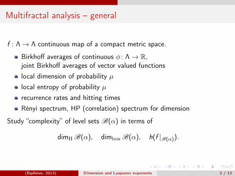
Multifractal analysis – general
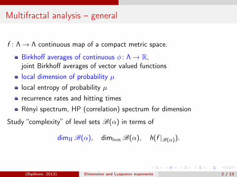
f : Λ→ Λ continuous map of a compact metric space.
Birkhoff averages of continuous φ : Λ→ R,joint Birkhoff averages of vector valued functionslocal dimension of probability µlocal entropy of probability µrecurrence rates and hitting timesRényi spectrum, HP (correlation) spectrum for dimension
Study “complexity” of level sets B(α) in terms of
dimH B(α), dimbox B(α), h(f |B(α)).
(Będlewo, 2013) Dimension and Lyapunov exponents 2 / 13
Multifractal analysis – general
[Besicovitch 34, Hentschel-Procaccia 83,Halsey-Jensen-Kadanoff-Procaccia-Shraiman 86, Collet-Lebowitz-Porcio 87,Rand 89, Lopes 89, Simpelaere 94, Olsen 95, Pesin-Tempelman 95,Pesin-Weiss 9*, Schmeling 99, Barreira–Saussol–Schmeling 9∗,Climenhaga 13,
Kesseböhmer-Stratmann 0∗, Byrne, Nakaishi 00, Pollicott-Weiss 01,Stratmann-Urbański 03, Yuri 04, Jordan-Rams 11]
(Będlewo, 2013) Dimension and Lyapunov exponents 3 / 13
Multifractal analysis – local dimension
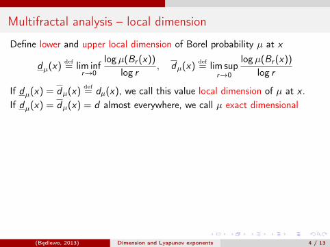
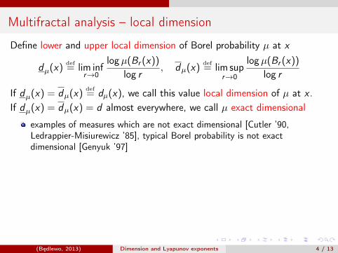
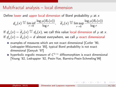
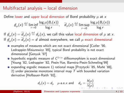
Define lower and upper local dimension of Borel probability µ at x
dµ(x)def= lim inf
r→0
logµ(Br (x))
log r, dµ(x)
def= lim sup
r→0
logµ(Br (x))
log r
If dµ(x) = dµ(x)def= dµ(x), we call this value local dimension of µ at x .
If dµ(x) = dµ(x) = d almost everywhere, we call µ exact dimensional
examples of measures which are not exact dimensional [Cutler ’90,Ledrappier-Misiurewicz ’85], typical Borel probability is not exactdimensional [Genyuk ’97]hyperbolic ergodic measure of C 1+α diffeomorphism is exact dimensional[Young ’82, Ledrappier ’82, Pesin-Yue, Barreira-Pesin-Schmeling’99]expanding ergodic measure 1) rational maps [Przytycki ’85, Mañé ’88],2) under piecewise monotone interval map T with bounded variationderivative [Hofbauer-Raith ’92],
dµ(x) = dµ µ-a.e.x and dµ =h(µ)
λ(µ)
(Będlewo, 2013) Dimension and Lyapunov exponents 4 / 13
Multifractal analysis – local dimension
Define lower and upper local dimension of Borel probability µ at x
dµ(x)def= lim inf
r→0
logµ(Br (x))
log r, dµ(x)
def= lim sup
r→0
logµ(Br (x))
log r
If dµ(x) = dµ(x)def= dµ(x), we call this value local dimension of µ at x .
If dµ(x) = dµ(x) = d almost everywhere, we call µ exact dimensional
examples of measures which are not exact dimensional [Cutler ’90,Ledrappier-Misiurewicz ’85], typical Borel probability is not exactdimensional [Genyuk ’97]
hyperbolic ergodic measure of C 1+α diffeomorphism is exact dimensional[Young ’82, Ledrappier ’82, Pesin-Yue, Barreira-Pesin-Schmeling’99]expanding ergodic measure 1) rational maps [Przytycki ’85, Mañé ’88],2) under piecewise monotone interval map T with bounded variationderivative [Hofbauer-Raith ’92],
dµ(x) = dµ µ-a.e.x and dµ =h(µ)
λ(µ)
(Będlewo, 2013) Dimension and Lyapunov exponents 4 / 13
Multifractal analysis – local dimension
Define lower and upper local dimension of Borel probability µ at x
dµ(x)def= lim inf
r→0
logµ(Br (x))
log r, dµ(x)
def= lim sup
r→0
logµ(Br (x))
log r
If dµ(x) = dµ(x)def= dµ(x), we call this value local dimension of µ at x .
If dµ(x) = dµ(x) = d almost everywhere, we call µ exact dimensional
examples of measures which are not exact dimensional [Cutler ’90,Ledrappier-Misiurewicz ’85], typical Borel probability is not exactdimensional [Genyuk ’97]hyperbolic ergodic measure of C 1+α diffeomorphism is exact dimensional[Young ’82, Ledrappier ’82, Pesin-Yue, Barreira-Pesin-Schmeling’99]
expanding ergodic measure 1) rational maps [Przytycki ’85, Mañé ’88],2) under piecewise monotone interval map T with bounded variationderivative [Hofbauer-Raith ’92],
dµ(x) = dµ µ-a.e.x and dµ =h(µ)
λ(µ)
(Będlewo, 2013) Dimension and Lyapunov exponents 4 / 13
Multifractal analysis – local dimension
Define lower and upper local dimension of Borel probability µ at x
dµ(x)def= lim inf
r→0
logµ(Br (x))
log r, dµ(x)
def= lim sup
r→0
logµ(Br (x))
log r
If dµ(x) = dµ(x)def= dµ(x), we call this value local dimension of µ at x .
If dµ(x) = dµ(x) = d almost everywhere, we call µ exact dimensional
examples of measures which are not exact dimensional [Cutler ’90,Ledrappier-Misiurewicz ’85], typical Borel probability is not exactdimensional [Genyuk ’97]hyperbolic ergodic measure of C 1+α diffeomorphism is exact dimensional[Young ’82, Ledrappier ’82, Pesin-Yue, Barreira-Pesin-Schmeling’99]expanding ergodic measure 1) rational maps [Przytycki ’85, Mañé ’88],2) under piecewise monotone interval map T with bounded variationderivative [Hofbauer-Raith ’92],
dµ(x) = dµ µ-a.e.x and dµ =h(µ)
λ(µ)
(Będlewo, 2013) Dimension and Lyapunov exponents 4 / 13
Multifractal analysis – local dimension
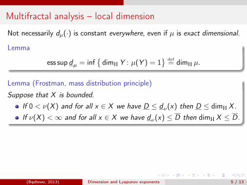
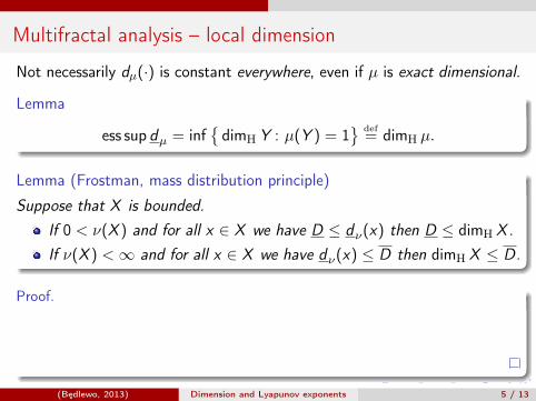
Not necessarily dµ(·) is constant everywhere, even if µ is exact dimensional.
Lemma
ess sup dµ = inf{dimH Y : µ(Y ) = 1
} def= dimH µ.
Lemma (Frostman, mass distribution principle)
Suppose that X is bounded.If 0 < ν(X ) and for all x ∈ X we have D ≤ dν(x) then D ≤ dimH X.If ν(X ) <∞ and for all x ∈ X we have dν(x) ≤ D then dimH X ≤ D.
Proof.
By [Falconer, Mattila]
0 <
µ(X ) ≤ Hc(X ),
where Hc(·) denotes the c-dimensional Hausdorff measure. So, ≤ dimH X .
(Będlewo, 2013) Dimension and Lyapunov exponents 5 / 13
Multifractal analysis – local dimension
Not necessarily dµ(·) is constant everywhere, even if µ is exact dimensional.
Lemma
ess sup dµ = inf{dimH Y : µ(Y ) = 1
} def= dimH µ.
Lemma (Frostman, mass distribution principle)
Suppose that X is bounded.If 0 < ν(X ) and for all x ∈ X we have D ≤ dν(x) then D ≤ dimH X.If ν(X ) <∞ and for all x ∈ X we have dν(x) ≤ D then dimH X ≤ D.
Proof.
By [Falconer, Mattila]
0 <
µ(X ) ≤ Hc(X ),
where Hc(·) denotes the c-dimensional Hausdorff measure. So, ≤ dimH X .
(Będlewo, 2013) Dimension and Lyapunov exponents 5 / 13

Multifractal analysis – local dimension
Not necessarily dµ(·) is constant everywhere, even if µ is exact dimensional.
Lemma
ess sup dµ = inf{dimH Y : µ(Y ) = 1
} def= dimH µ.
Lemma (Frostman, mass distribution principle)
Suppose that X is bounded.If 0 < ν(X ) and for all x ∈ X we have D ≤ dν(x) then D ≤ dimH X.If ν(X ) <∞ and for all x ∈ X we have dν(x) ≤ D then dimH X ≤ D.
Proof.
If for c < D and r small we have log µ(Br (x)) < c log r
By [Falconer, Mattila]
0 <
µ(X ) ≤ Hc(X ),
where Hc(·) denotes the c-dimensional Hausdorff measure. So, ≤ dimH X .
(Będlewo, 2013) Dimension and Lyapunov exponents 5 / 13

Multifractal analysis – local dimension
Not necessarily dµ(·) is constant everywhere, even if µ is exact dimensional.
Lemma
ess sup dµ = inf{dimH Y : µ(Y ) = 1
} def= dimH µ.
Lemma (Frostman, mass distribution principle)
Suppose that X is bounded.If 0 < ν(X ) and for all x ∈ X we have D ≤ dν(x) then D ≤ dimH X.If ν(X ) <∞ and for all x ∈ X we have dν(x) ≤ D then dimH X ≤ D.
Proof.
If for c < D and r small we have µ(B(x , r)) < r c
By [Falconer, Mattila]
0 <
µ(X ) ≤ Hc(X ),
where Hc(·) denotes the c-dimensional Hausdorff measure. So, ≤ dimH X .
(Będlewo, 2013) Dimension and Lyapunov exponents 5 / 13

Multifractal analysis – local dimension
Not necessarily dµ(·) is constant everywhere, even if µ is exact dimensional.
Lemma
ess sup dµ = inf{dimH Y : µ(Y ) = 1
} def= dimH µ.
Lemma (Frostman, mass distribution principle)
Suppose that X is bounded.If 0 < ν(X ) and for all x ∈ X we have D ≤ dν(x) then D ≤ dimH X.If ν(X ) <∞ and for all x ∈ X we have dν(x) ≤ D then dimH X ≤ D.
Proof.
If for c < D and r small we have µ(B(x , r)) < r c then µ(Br (x))rc < 1.
By[Falconer, Mattila]
0 <
µ(X ) ≤ Hc(X ),
where Hc(·) denotes the c-dimensional Hausdorff measure. So, ≤ dimH X .
(Będlewo, 2013) Dimension and Lyapunov exponents 5 / 13
Multifractal analysis – local dimension
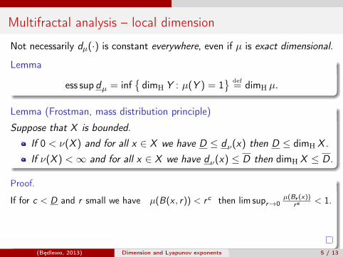
Not necessarily dµ(·) is constant everywhere, even if µ is exact dimensional.
Lemma
ess sup dµ = inf{dimH Y : µ(Y ) = 1
} def= dimH µ.
Lemma (Frostman, mass distribution principle)
Suppose that X is bounded.If 0 < ν(X ) and for all x ∈ X we have D ≤ dν(x) then D ≤ dimH X.If ν(X ) <∞ and for all x ∈ X we have dν(x) ≤ D then dimH X ≤ D.
Proof.
If for c < D and r small we have µ(B(x , r)) < r c then lim supr→0µ(Br (x))
rc < 1.
By [Falconer, Mattila]
0 <
µ(X ) ≤ Hc(X ),
where Hc(·) denotes the c-dimensional Hausdorff measure. So, ≤ dimH X .
(Będlewo, 2013) Dimension and Lyapunov exponents 5 / 13
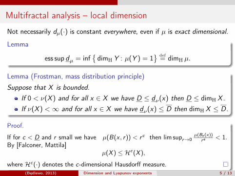
Multifractal analysis – local dimension
Not necessarily dµ(·) is constant everywhere, even if µ is exact dimensional.
Lemma
ess sup dµ = inf{dimH Y : µ(Y ) = 1
} def= dimH µ.
Lemma (Frostman, mass distribution principle)
Suppose that X is bounded.If 0 < ν(X ) and for all x ∈ X we have D ≤ dν(x) then D ≤ dimH X.If ν(X ) <∞ and for all x ∈ X we have dν(x) ≤ D then dimH X ≤ D.
Proof.
If for c < D and r small we have µ(B(x , r)) < r c then lim supr→0µ(Br (x))
rc < 1.By [Falconer, Mattila]
0 <
µ(X ) ≤ Hc(X ),
where Hc(·) denotes the c-dimensional Hausdorff measure.
So, ≤ dimH X .
(Będlewo, 2013) Dimension and Lyapunov exponents 5 / 13

Multifractal analysis – local dimension
Not necessarily dµ(·) is constant everywhere, even if µ is exact dimensional.
Lemma
ess sup dµ = inf{dimH Y : µ(Y ) = 1
} def= dimH µ.
Lemma (Frostman, mass distribution principle)
Suppose that X is bounded.If 0 < ν(X ) and for all x ∈ X we have D ≤ dν(x) then D ≤ dimH X.If ν(X ) <∞ and for all x ∈ X we have dν(x) ≤ D then dimH X ≤ D.
Proof.
If for c < D and r small we have µ(B(x , r)) < r c then lim supr→0µ(Br (x))
rc < 1.By [Falconer, Mattila]
0 < µ(X ) ≤ Hc(X ),
where Hc(·) denotes the c-dimensional Hausdorff measure. So, c ≤ dimH X .(Będlewo, 2013) Dimension and Lyapunov exponents 5 / 13
Multifractal analysis – local dimension
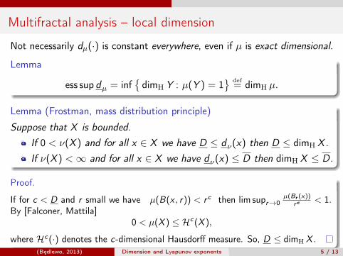
Not necessarily dµ(·) is constant everywhere, even if µ is exact dimensional.
Lemma
ess sup dµ = inf{dimH Y : µ(Y ) = 1
} def= dimH µ.
Lemma (Frostman, mass distribution principle)
Suppose that X is bounded.If 0 < ν(X ) and for all x ∈ X we have D ≤ dν(x) then D ≤ dimH X.If ν(X ) <∞ and for all x ∈ X we have dν(x) ≤ D then dimH X ≤ D.
Proof.
If for c < D and r small we have µ(B(x , r)) < r c then lim supr→0µ(Br (x))
rc < 1.By [Falconer, Mattila]
0 < µ(X ) ≤ Hc(X ),
where Hc(·) denotes the c-dimensional Hausdorff measure. So, D ≤ dimH X .(Będlewo, 2013) Dimension and Lyapunov exponents 5 / 13
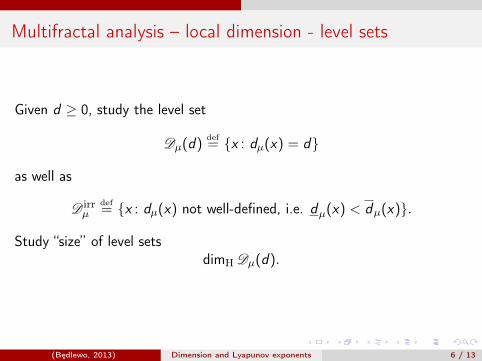
Multifractal analysis – local dimension - level sets
Given d ≥ 0, study the level set
Dµ(d)def= {x : dµ(x) = d}
as well as
D irrµ
def= {x : dµ(x) not well-defined, i.e. dµ(x) < dµ(x)}.
Study “size” of level setsdimH Dµ(d).
(Będlewo, 2013) Dimension and Lyapunov exponents 6 / 13
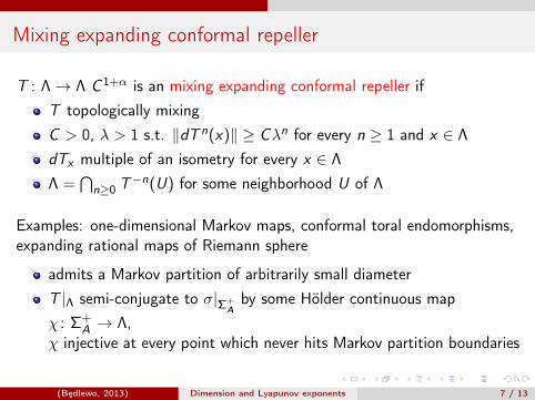
Mixing expanding conformal repeller
T : Λ→ Λ C 1+α is an mixing expanding conformal repeller ifT topologically mixingC > 0, λ > 1 s.t. ‖dT n(x)‖ ≥ Cλn for every n ≥ 1 and x ∈ Λ
dTx multiple of an isometry for every x ∈ Λ
Λ =⋂
n≥0 T−n(U) for some neighborhood U of Λ
Examples: one-dimensional Markov maps, conformal toral endomorphisms,expanding rational maps of Riemann sphere
admits a Markov partition of arbitrarily small diameterT |Λ semi-conjugate to σ|Σ+
Aby some Hölder continuous map
χ : Σ+A → Λ,
χ injective at every point which never hits Markov partition boundaries
(Będlewo, 2013) Dimension and Lyapunov exponents 7 / 13
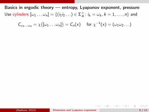
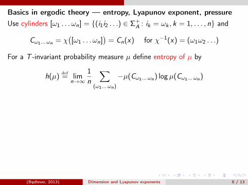
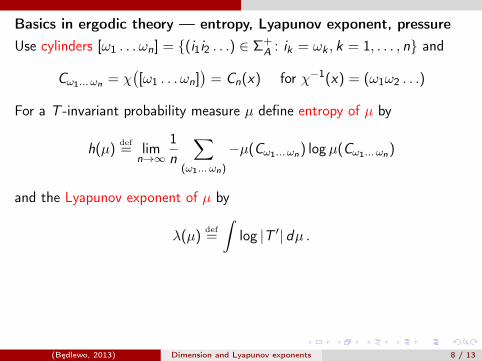
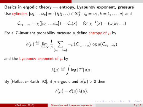
Basics in ergodic theory — entropy, Lyapunov exponent, pressureUse cylinders [ω1 . . . ωn] = {(i1i2 . . .) ∈ Σ+
A : ik = ωk , k = 1, . . . , n} and
Cω1... ωn = χ([ω1 . . . ωn]
)= Cn(x) for χ−1(x) = (ω1ω2 . . .)
For a T -invariant probability measure µ define entropy of µ by
h(µ)def= lim
n→∞
1n
∑(ω1... ωn)
−µ(Cω1... ωn) logµ(Cω1... ωn)
and the Lyapunov exponent of µ by
λ(µ)def=
∫log |T ′| dµ .
By [Hofbauer-Raith ’92], if µ ergodic and λ(µ) > 0 then
h(µ) = d(µ)λ(µ).
(Będlewo, 2013) Dimension and Lyapunov exponents 8 / 13
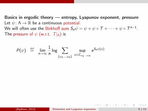
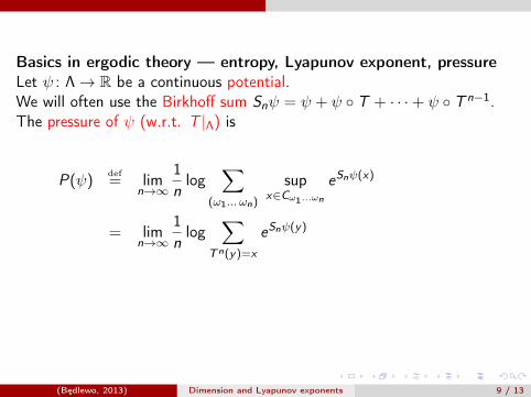
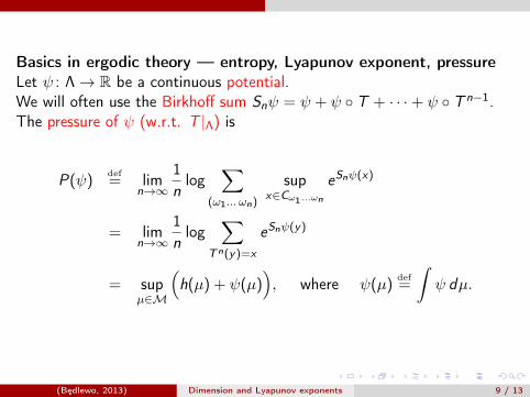
Basics in ergodic theory — entropy, Lyapunov exponent, pressureLet ψ : Λ→ R be a continuous potential.We will often use the Birkhoff sum Snψ = ψ + ψ ◦ T + · · ·+ ψ ◦ T n−1.The pressure of ψ (w.r.t. T |Λ) is
P(ψ)def= lim
n→∞
1nlog
∑(ω1... ωn)
supx∈Cω1...ωn
eSnψ(x)
= limn→∞
1nlog
∑Tn(y)=x
eSnψ(y)
= supµ∈M
(h(µ) + ψ(µ)
), where ψ(µ)
def=
∫ψ dµ.
(Będlewo, 2013) Dimension and Lyapunov exponents 9 / 13
Basics in ergodic theory — normalized potential
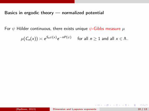
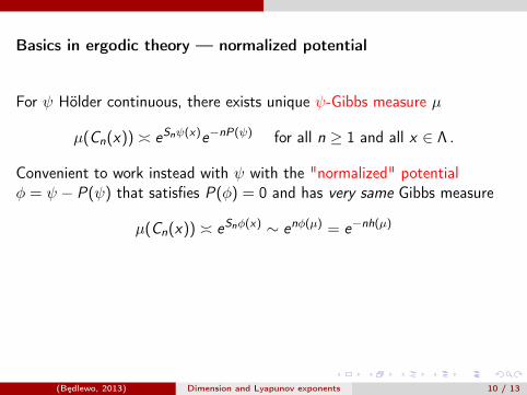
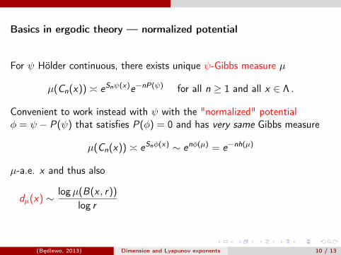
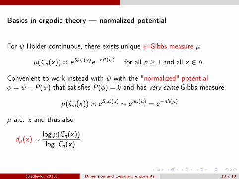
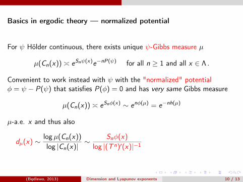
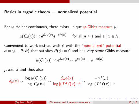
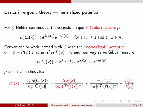
For ψ Hölder continuous, there exists unique ψ-Gibbs measure µ
µ(Cn(x)) � eSnψ(x)e−nP(ψ) for all n ≥ 1 and all x ∈ Λ .
Convenient to work instead with ψ with the "normalized" potentialφ = ψ − P(ψ) that satisfies P(φ) = 0 and has very same Gibbs measure
µ(Cn(x)) � eSnφ(x) ∼ enφ(µ) = e−nh(µ)
µ-a.e. x and thus also
dµ(x)
∼ Snφ(x)
log |(T n)′(x)|−1 ∼−n h(µ)
log |(T n)′(x)|−1 ∼h(µ)
λ(µ)
(Będlewo, 2013) Dimension and Lyapunov exponents 10 / 13
Basics in ergodic theory — normalized potential
For ψ Hölder continuous, there exists unique ψ-Gibbs measure µ
µ(Cn(x)) � eSnψ(x)e−nP(ψ) for all n ≥ 1 and all x ∈ Λ .
Convenient to work instead with ψ with the "normalized" potentialφ = ψ − P(ψ) that satisfies P(φ) = 0 and has very same Gibbs measure
µ(Cn(x)) � eSnφ(x) ∼ enφ(µ) = e−nh(µ)
µ-a.e. x and thus also
dµ(x) ∼ logµ(B(x , r))
log r
∼ Snφ(x)
log |(T n)′(x)|−1 ∼−n h(µ)
log |(T n)′(x)|−1 ∼h(µ)
λ(µ)
(Będlewo, 2013) Dimension and Lyapunov exponents 10 / 13
Basics in ergodic theory — normalized potential
For ψ Hölder continuous, there exists unique ψ-Gibbs measure µ
µ(Cn(x)) � eSnψ(x)e−nP(ψ) for all n ≥ 1 and all x ∈ Λ .
Convenient to work instead with ψ with the "normalized" potentialφ = ψ − P(ψ) that satisfies P(φ) = 0 and has very same Gibbs measure
µ(Cn(x)) � eSnφ(x) ∼ enφ(µ) = e−nh(µ)
µ-a.e. x and thus also
dµ(x) ∼ logµ(Cn(x))
log |Cn(x)|
∼ Snφ(x)
log |(T n)′(x)|−1 ∼−n h(µ)
log |(T n)′(x)|−1 ∼h(µ)
λ(µ)
(Będlewo, 2013) Dimension and Lyapunov exponents 10 / 13
Basics in ergodic theory — normalized potential
For ψ Hölder continuous, there exists unique ψ-Gibbs measure µ
µ(Cn(x)) � eSnψ(x)e−nP(ψ) for all n ≥ 1 and all x ∈ Λ .
Convenient to work instead with ψ with the "normalized" potentialφ = ψ − P(ψ) that satisfies P(φ) = 0 and has very same Gibbs measure
µ(Cn(x)) � eSnφ(x) ∼ enφ(µ) = e−nh(µ)
µ-a.e. x and thus also
dµ(x) ∼ logµ(Cn(x))
log |Cn(x)|∼ Snφ(x)
log |(T n)′(x)|−1
∼ −n h(µ)
log |(T n)′(x)|−1 ∼h(µ)
λ(µ)
(Będlewo, 2013) Dimension and Lyapunov exponents 10 / 13
Basics in ergodic theory — normalized potential
For ψ Hölder continuous, there exists unique ψ-Gibbs measure µ
µ(Cn(x)) � eSnψ(x)e−nP(ψ) for all n ≥ 1 and all x ∈ Λ .
Convenient to work instead with ψ with the "normalized" potentialφ = ψ − P(ψ) that satisfies P(φ) = 0 and has very same Gibbs measure
µ(Cn(x)) � eSnφ(x) ∼ enφ(µ) = e−nh(µ)
µ-a.e. x and thus also
dµ(x) ∼ logµ(Cn(x))
log |Cn(x)|∼ Snφ(x)
log |(T n)′(x)|−1 ∼−n h(µ)
log |(T n)′(x)|−1
∼ h(µ)
λ(µ)
(Będlewo, 2013) Dimension and Lyapunov exponents 10 / 13
Basics in ergodic theory — normalized potential
For ψ Hölder continuous, there exists unique ψ-Gibbs measure µ
µ(Cn(x)) � eSnψ(x)e−nP(ψ) for all n ≥ 1 and all x ∈ Λ .
Convenient to work instead with ψ with the "normalized" potentialφ = ψ − P(ψ) that satisfies P(φ) = 0 and has very same Gibbs measure
µ(Cn(x)) � eSnφ(x) ∼ enφ(µ) = e−nh(µ)
µ-a.e. x and thus also
dµ(x) ∼ logµ(Cn(x))
log |Cn(x)|∼ Snφ(x)
log |(T n)′(x)|−1 ∼−n h(µ)
log |(T n)′(x)|−1 ∼h(µ)
λ(µ)
(Będlewo, 2013) Dimension and Lyapunov exponents 10 / 13
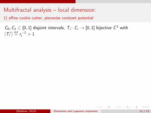
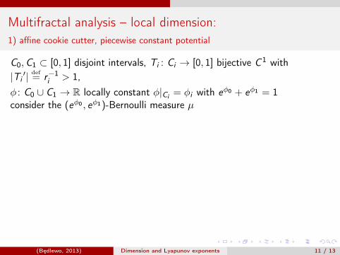
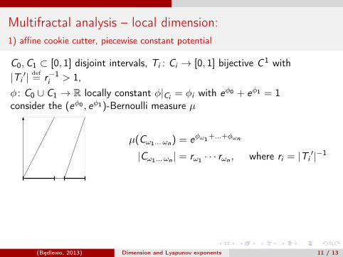
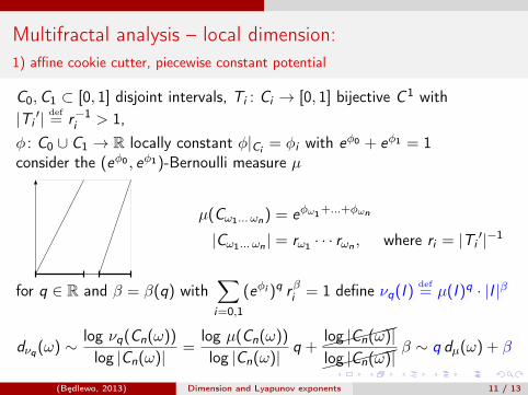
Multifractal analysis – local dimension:1) affine cookie cutter, piecewise constant potential
C0,C1 ⊂ [0, 1] disjoint intervals, Ti : Ci → [0, 1] bijective C 1 with|Ti′| def
= r−1i > 1
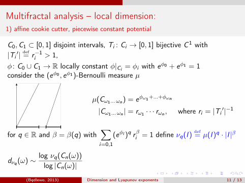
,φ : C0 ∪ C1 → R locally constant φ|Ci = φi with eφ0 + eφ1 = 1consider the (eφ0 , eφ1)-Bernoulli measure µ
µ(Cω1... ωn) = eφω1+...+φωn
|Cω1... ωn | = rω1 · · · rωn , where ri = |Ti′|−1
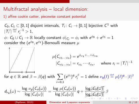
for q ∈ R and β = β(q) with∑i=0,1
(eφi )q rβi = 1 define νq(I )def= µ(I )q · |I |β
dνq (ω) ∼ log νq(Cn(ω))
log |Cn(ω)|=
log µ(Cn(ω))
log |Cn(ω)|q + ������log |Cn(ω)|
������log |Cn(ω)|β ∼ q dµ(ω) + β
(Będlewo, 2013) Dimension and Lyapunov exponents 11 / 13
Multifractal analysis – local dimension:1) affine cookie cutter, piecewise constant potential
C0,C1 ⊂ [0, 1] disjoint intervals, Ti : Ci → [0, 1] bijective C 1 with|Ti′| def
= r−1i > 1,
φ : C0 ∪ C1 → R locally constant φ|Ci = φi with eφ0 + eφ1 = 1consider the (eφ0 , eφ1)-Bernoulli measure µ
µ(Cω1... ωn) = eφω1+...+φωn
|Cω1... ωn | = rω1 · · · rωn , where ri = |Ti′|−1
for q ∈ R and β = β(q) with∑i=0,1
(eφi )q rβi = 1 define νq(I )def= µ(I )q · |I |β
dνq (ω) ∼ log νq(Cn(ω))
log |Cn(ω)|
=log µ(Cn(ω))
log |Cn(ω)|q + ������log |Cn(ω)|
������log |Cn(ω)|β ∼ q dµ(ω) + β
(Będlewo, 2013) Dimension and Lyapunov exponents 11 / 13
Multifractal analysis – local dimension:1) affine cookie cutter, piecewise constant potential
C0,C1 ⊂ [0, 1] disjoint intervals, Ti : Ci → [0, 1] bijective C 1 with|Ti′| def
= r−1i > 1,
φ : C0 ∪ C1 → R locally constant φ|Ci = φi with eφ0 + eφ1 = 1consider the (eφ0 , eφ1)-Bernoulli measure µ
µ(Cω1... ωn) = eφω1+...+φωn
|Cω1... ωn | = rω1 · · · rωn , where ri = |Ti′|−1
for q ∈ R and β = β(q) with∑i=0,1
(eφi )q rβi = 1 define νq(I )def= µ(I )q · |I |β
dνq (ω) ∼ log νq(Cn(ω))
log |Cn(ω)|=
log µ(Cn(ω))
log |Cn(ω)|q + ������log |Cn(ω)|
������log |Cn(ω)|β
∼ q dµ(ω) + β
(Będlewo, 2013) Dimension and Lyapunov exponents 11 / 13
Multifractal analysis – local dimension:1) affine cookie cutter, piecewise constant potential
C0,C1 ⊂ [0, 1] disjoint intervals, Ti : Ci → [0, 1] bijective C 1 with|Ti′| def
= r−1i > 1,
φ : C0 ∪ C1 → R locally constant φ|Ci = φi with eφ0 + eφ1 = 1consider the (eφ0 , eφ1)-Bernoulli measure µ
µ(Cω1... ωn) = eφω1+...+φωn
|Cω1... ωn | = rω1 · · · rωn , where ri = |Ti′|−1
for q ∈ R and β = β(q) with∑i=0,1
(eφi )q rβi = 1 define νq(I )def= µ(I )q · |I |β
dνq (ω) ∼ log νq(Cn(ω))
log |Cn(ω)|=
log µ(Cn(ω))
log |Cn(ω)|q + ������log |Cn(ω)|
������log |Cn(ω)|β ∼ q dµ(ω) + β
(Będlewo, 2013) Dimension and Lyapunov exponents 11 / 13
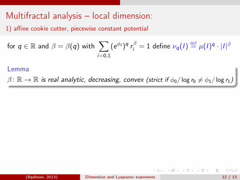
Multifractal analysis – local dimension:1) affine cookie cutter, piecewise constant potential
for q ∈ R and β = β(q) with∑i=0,1
(eφi )q rβi = 1 define νq(I )def= µ(I )q · |I |β
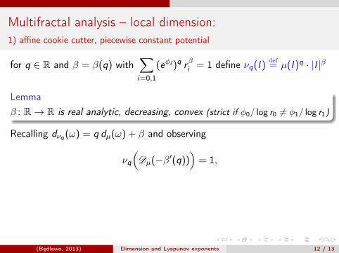
Lemmaβ : R→ R is real analytic, decreasing, convex (strict if φ0/ log r0 6= φ1/ log r1)
Recalling dνq (ω) = q dµ(ω) + β and observing
νq
(Dµ(−β′(q))
)= 1,
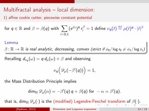
the Mass Distribution Principle implies
dimH Dµ(α) = −β′(q) q + β(q) for − α = β′(q).
that is, dimH Dµ(·) is the (modified) Legendre-Fenchel transform of β(·).
(Będlewo, 2013) Dimension and Lyapunov exponents 12 / 13
Multifractal analysis – local dimension:1) affine cookie cutter, piecewise constant potential
for q ∈ R and β = β(q) with∑i=0,1
(eφi )q rβi = 1 define νq(I )def= µ(I )q · |I |β
Lemmaβ : R→ R is real analytic, decreasing, convex (strict if φ0/ log r0 6= φ1/ log r1)
Recalling dνq (ω) = q dµ(ω) + β and observing
νq
(Dµ(−β′(q))
)= 1,
the Mass Distribution Principle implies
dimH Dµ(α) = −β′(q) q + β(q) for − α = β′(q).
that is, dimH Dµ(·) is the (modified) Legendre-Fenchel transform of β(·).(Będlewo, 2013) Dimension and Lyapunov exponents 12 / 13
Multifractal analysis – local dimension:Legendre-Fenchel transform
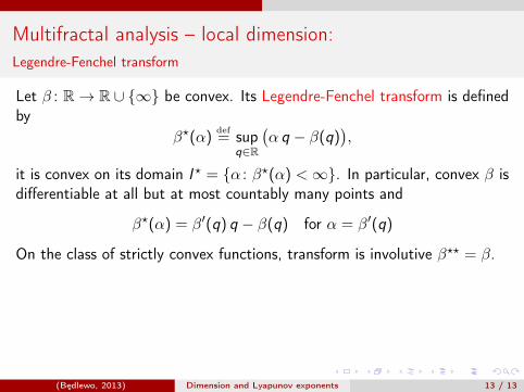
Let β : R→ R ∪ {∞} be convex. Its Legendre-Fenchel transform is definedby
β?(α)def= sup
q∈R
(α q − β(q)
),
it is convex on its domain I ? = {α : β?(α) <∞}. In particular, convex β isdifferentiable at all but at most countably many points and
β?(α) = β′(q) q − β(q) for α = β′(q)
On the class of strictly convex functions, transform is involutive β?? = β.
Formally, the function fµ(α)def= − dimH Dµ(−α) is the Legendre-Fenchel
transform of β, but it is a common practice to address Dµ by this name
dimH Dµ(α) = infp∈R
(α p + β(p)) = −β′(q) q + β(q) for α = −β′(q).
(Będlewo, 2013) Dimension and Lyapunov exponents 13 / 13
Multifractal analysis – local dimension:Legendre-Fenchel transform
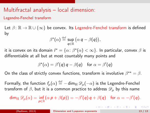
Let β : R→ R ∪ {∞} be convex. Its Legendre-Fenchel transform is definedby
β?(α)def= sup
q∈R
(α q − β(q)
),
it is convex on its domain I ? = {α : β?(α) <∞}. In particular, convex β isdifferentiable at all but at most countably many points and
β?(α) = β′(q) q − β(q) for α = β′(q)
On the class of strictly convex functions, transform is involutive β?? = β.
Formally, the function fµ(α)def= − dimH Dµ(−α) is the Legendre-Fenchel
transform of β, but it is a common practice to address Dµ by this name
dimH Dµ(α) = infp∈R
(α p + β(p)) = −β′(q) q + β(q) for α = −β′(q).
(Będlewo, 2013) Dimension and Lyapunov exponents 13 / 13


![Lyapunov exponents for Quantum Channels: an entropy ...mat.ufrgs.br/~alopes/Lyapunov-exp-quantum-26-jun.pdf · For a xed and a general Lit was presented in [12] a natural concept](https://static.fdocument.org/doc/165x107/5f646c0164fb447c6567564f/lyapunov-exponents-for-quantum-channels-an-entropy-matufrgsbralopeslyapunov-exp-quantum-26-junpdf.jpg)