Konstanz, 07.01.2009

Digital Signal ProcessingWS 2009/10

Lab Sheet 9 – Solution

Exercise 1 (6)

Determine the power spectrum of a stationary stochastic signal X[n] whose autocorre-lation is given as

φxx[m] = σ2xe−a|m|, a ∈ R

How does the phase of the power spectrum look like?

Φxx

(eiω

)=

σ2x (1− e−2a)

1− 2e−a cos (ω) + e−2a∈ R

The autocorrelation of a stationary (real-valued) signal is always even and hence thephase of the power spectrum is always 0.

Exercise 2 (15)

An audio signal x(t) is generated by a loudspeaker and gets reflected at a wall with areflection coefficient r. A microphone next to the loudspeaker records a signal y(t). Aftersampling

y[n] = x[n] + rx[n− k]

applies, where k is the delay of the echo.

a) Determine the autocorrelation φyy[l] given the autocorrelation φxx[l]. (5)

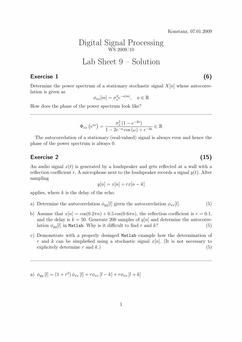
b) Assume that x[n] = cos(0.2πn) + 0.5 cos(0.6πn), the reflection coefficient is r = 0.1,and the delay is k = 50. Generate 200 samples of y[n] and determine the autocorre-lation φyy[l] in Matlab. Why is it difficult to find r and k? (5)

c) Demonstrate with a properly desinged Matlab example how the determination ofr and k can be simpliefied using a stochastic signal x[n]. (It is not necessary toexplicitely determine r and k.) (5)

a) φyy [l] = (1 + r2)φxx [l] + rφxx [l − k] + rφxx [l + k]

1

b) %Generate 200 samplesn=0:200;r=0.1;k=50;x=cos(0.02*pi*n)+0.05*cos(0.6*pi*n);len = length(x);echo = zeros(1,len);echo(k:len) = r*x(1:len-(k-1));y=x+echo;figure(1)subplot(211)plot([x’ y’ echo’])legend(’x’,’y’,’echo’)xlabel(’index n’)ylabel(’amplitude’);subplot(212)phiyy = xcorr(y, ’unbiased’); %Normalizes correlation (see Matlab help)plot(phiyy(len:2*(len)-1))ylabel(’phi_yy’);xlabel(’index l’);

0 50 100 150 200 250−1.5

−1

−0.5

0

0.5

1

1.5

index n

ampl

itude

0 50 100 150 200 250−0.5

0

0.5

1

phi yy

index l

xyecho

It is difficult to determine r and k because of the autocorrelation of the input signalx [n].

2

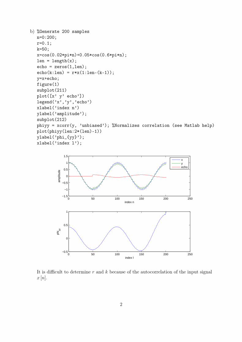
c) n = 0:10000; % more samples improve the accuracy of the estimationr = 0.1;k = 50;len = length(n);x = (rand(1,len)-0.5).*2*sqrt(3); %uniform distribution with mean=0 andvariance 1phixx = xcorr(x, ’unbiased’); % should be close to delta[l]echo = zeros(1, len);echo(k:len)=r*x(1:(len-(k-1)));y = x+echo;maxlags = 100;phiyy = xcorr(y, maxlags, ’unbiased’); % compute correlation for lag <100

figure(2)subplot(211)stem((-len+1):(len-1),phixx,’.’)xlabel(’l’); ylabel(’phi_xx’)grid onsubplot(212)stem((-maxlags):(maxlags),phiyy,’.’) xlabel(’l’) ylabel(’phi_yy’)grid on

−1 −0.8 −0.6 −0.4 −0.2 0 0.2 0.4 0.6 0.8 1

x 104

−1

−0.5

0

0.5

1

1.5

l

phi xx

−100 −80 −60 −40 −20 0 20 40 60 80 100−0.5

0

0.5

1

1.5

l

phi yy

3

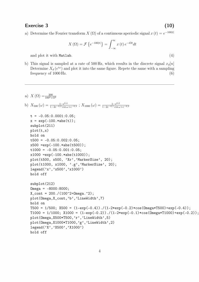
Exercise 3 (10)

a) Determine the Fourier transformX (Ω) of a continuous aperiodic signal x (t) = e−100|t|

X (Ω) = Fe−100|t| =

ˆ ∞−∞

x (t) e−iΩtdt

and plot it with Matlab. (4)

b) This signal is sampled at a rate of 500Hz, which results in the discrete signal xd[n]Determine Xd (eiω) and plot it into the same figure. Repete the same with a samplingfrequency of 1000Hz. (6)

a) X (Ω) = 2001002+Ω2

b) X500 (ω) = 1−e0,4

1−2e−0,2 cos ω+e−0,4 ; X1000 (ω) = 1−e0,2

1−2e−0,1 cos ω+e−0,2

t = -0.05:0.0001:0.05;x = exp(-100.*abs(t));subplot(211)plot(t,x)hold ont500 = -0.05:0.002:0.05;x500 =exp(-100.*abs(t500));t1000 = -0.05:0.001:0.05;x1000 =exp(-100.*abs(t1000));plot(t500, x500, ’Xr’,’MarkerSize’, 20);plot(t1000, x1000, ’.g’,’MarkerSize’, 20);legend(’x’,’x500’,’x1000’)hold off

subplot(212)Omega = -8000:8000;X_cont = 200./(100^2+Omega.^2);plot(Omega,X_cont,’b’,’LineWidth’,7)hold onT500 = 1/500; X500 = (1-exp(-0.4))./(1-2*exp(-0.2)*cos(Omega*T500)+exp(-0.4));T1000 = 1/1000; X1000 = (1-exp(-0.2))./(1-2*exp(-0.1)*cos(Omega*T1000)+exp(-0.2));plot(Omega,X500*T500,’r’,’LineWidth’,5)plot(Omega,X1000*T1000,’g’,’LineWidth’,2)legend(’X’,’X500’,’X1000’)hold off

4

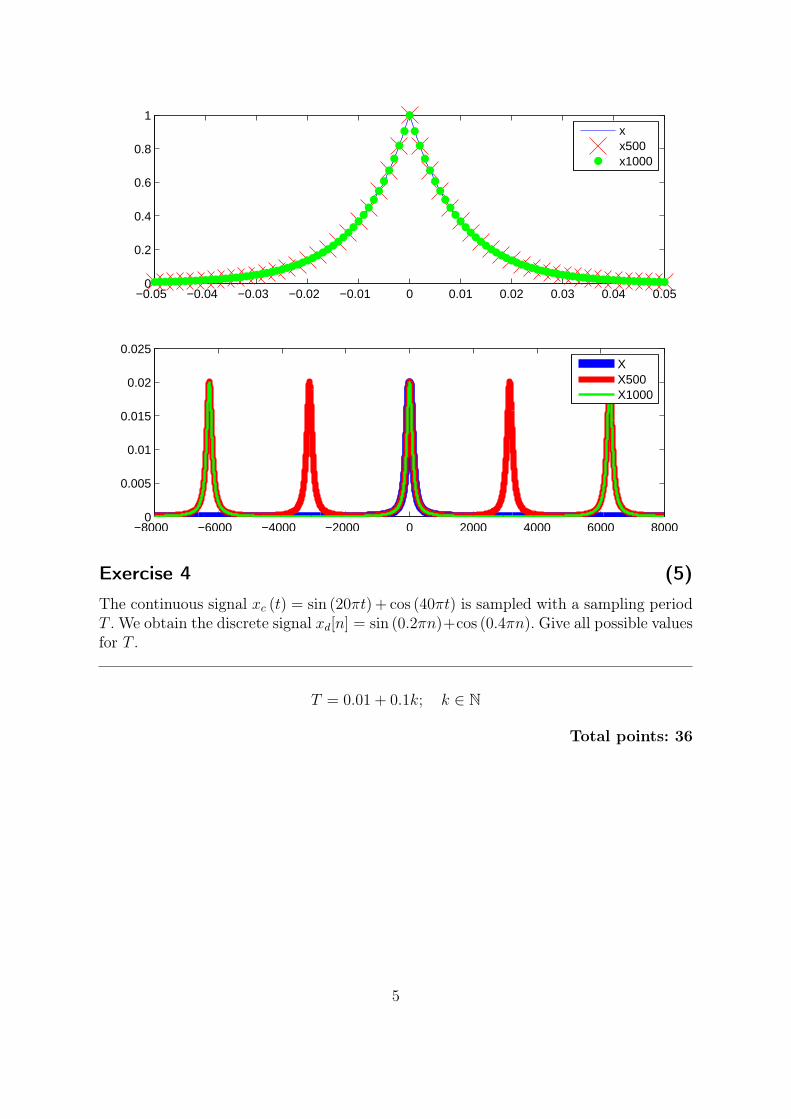
−0.05 −0.04 −0.03 −0.02 −0.01 0 0.01 0.02 0.03 0.04 0.050

0.2

0.4

0.6

0.8

1

xx500x1000

−8000 −6000 −4000 −2000 0 2000 4000 6000 80000

0.005

0.01

0.015

0.02

0.025

XX500X1000

Exercise 4 (5)

The continuous signal xc (t) = sin (20πt) + cos (40πt) is sampled with a sampling periodT . We obtain the discrete signal xd[n] = sin (0.2πn)+cos (0.4πn). Give all possible valuesfor T .

T = 0.01 + 0.1k; k ∈ N

Total points: 36

5