DIGITAL SIGNAL ROCESSING LECTURE 3 - University of...
35
DIGITAL SIGNAL PROCESSING LECTURE 3 Fall 2010 2K8-5 th Semester Tahir Muhammad Tahir Muhammad [email protected] Content and Figures are from Discrete-Time Signal Processing, 2e by Oppenheim, Shafer, and Buck, ©1999-2000 Prentice Hall Inc.
Transcript of DIGITAL SIGNAL ROCESSING LECTURE 3 - University of...
DIGITAL SIGNAL PROCESSINGLECTURE 3Fall 20102K8-5th SemesterTahir MuhammadTahir [email protected]
Content and Figures are from Discrete-Time Signal Processing, 2e by Oppenheim, Shafer, and
Buck, ©1999-2000 Prentice Hall Inc.
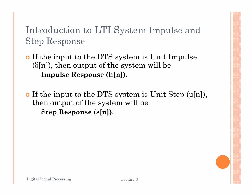
Introduction to LTI System Impulse and Step Response
If the input to the DTS system is Unit Impulse p y p(δ[n]), then output of the system will be
Impulse Response (h[n]).
If the input to the DTS system is Unit Step (µ[n]), then output of the system will be
S R ( [ ])Step Response (s[n]).
Digital Signal Processing 2Lecture 3
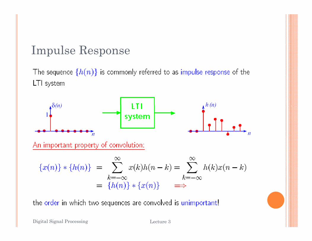
Impulse Response
Digital Signal Processing 3Lecture 3
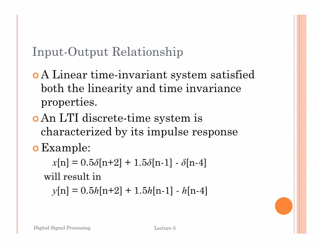
Input-Output Relationship
A Linear time-invariant system satisfied A Linear time invariant system satisfied both the linearity and time invariance properties.An LTI discrete-time system is characterized by its impulse responseExample:x[n] = 0.5δ[n+2] + 1.5δ[n-1] - δ[n-4]
will result iny[n] = 0.5h[n+2] + 1.5h[n-1] - h[n-4]
Digital Signal Processing 4Lecture 3
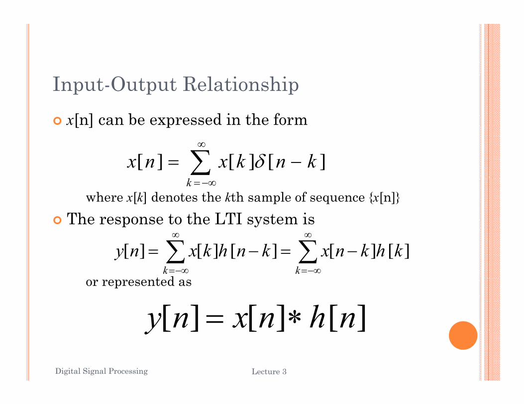
Input-Output Relationshipx[n] can be expressed in the form[ ] p
∑∞
−= knkxnx ][][][ δ
where x[k] denotes the kth sample of sequence {x[n]}The response to the LTI system is
−∞=k
t d
∑∑∞
−∞=
∞
−∞=
−=−=kk
khknxknhkxny ][][][][][or represented as
][][][ nhnxny ∗=Digital Signal Processing 5Lecture 3
][][][y
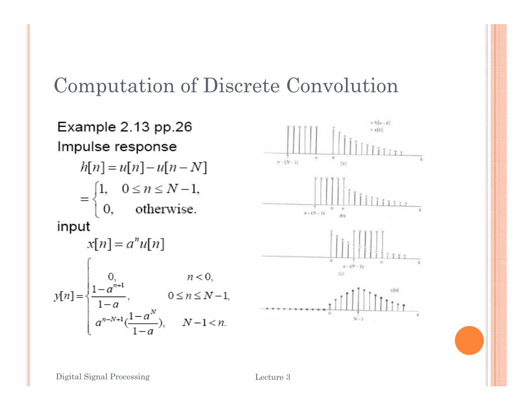
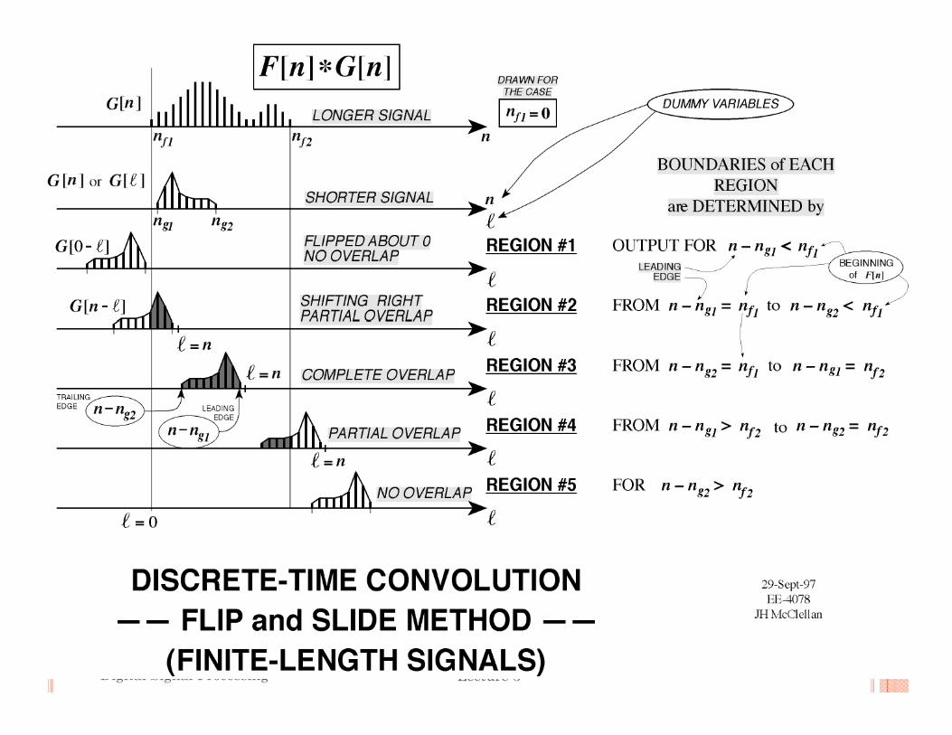
Computation of Discrete Convolution
Digital Signal Processing 6Lecture 3
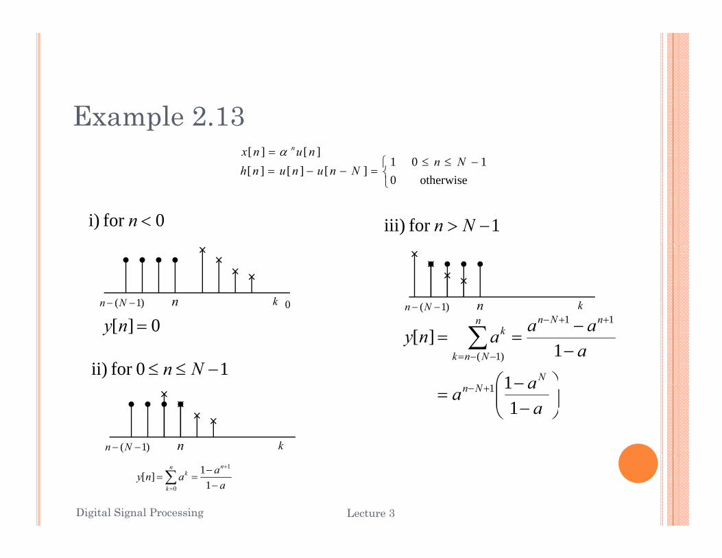
Example 2.13
⎨⎧ −≤≤
=−−=101
][][][Nn
Nnununh][][ nunx nα=
⎩⎨ otherwise0
][][][ Nnununh
0for i) <n 1for iii) −> Nn
kn)1( −− Nn kn)1( −− Nn0
0][ =ny
10for ii) −≤≤ Nn⎞
⎜⎛ −
−−
==++−
−−=∑
a
aaaany
NN
nNnn
Nnk
k
1
1][
1
11
)1(
kn)1( −− Nn
⎟⎠
⎞⎜⎜⎝
⎛−
= +−
aaa Nn
111
Digital Signal Processing 7Lecture 3
aaanynn
k
k
−−
==+
=∑ 1
1][1
0
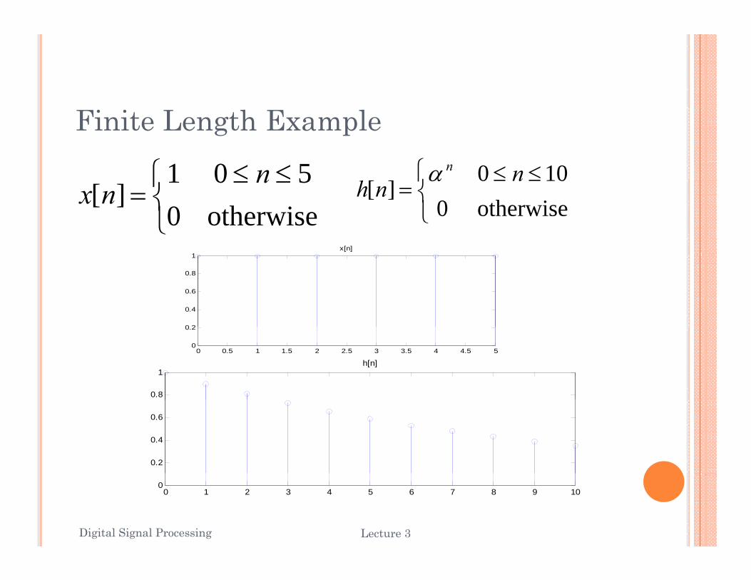
Finite Length Example
⎨⎧ ≤≤ 100 n
hnα⎧ ≤≤ 501 n
⎩⎨⎧ ≤≤
=otherwise0
100][
nnh
α
⎩⎨⎧ ≤≤
=otherwise0
501][
nnx
1x[n]
0 2
0.4
0.6
0.8
1
0.8
1h[n]
0 0.5 1 1.5 2 2.5 3 3.5 4 4.5 50
0.2
0.2
0.4
0.6
Digital Signal Processing 8Lecture 3
0 1 2 3 4 5 6 7 8 9 100
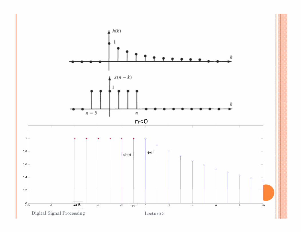
n<0
0.8
1
x[n-k]h[n]
0 2
0.4
0.6
Digital Signal Processing Lecture 3 9-10 -8 -6 -4 -2 0 2 4 6 8 100
0.2
nn-5
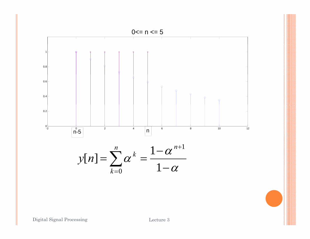
0<= n <= 5
0.8
1
0.4
0.6
-2 0 2 4 6 8 10 120
0.2
nn-5
αα −==
+
∑ 11][
1nnkny
α−=∑ 10k
Digital Signal Processing Lecture 3 10
1
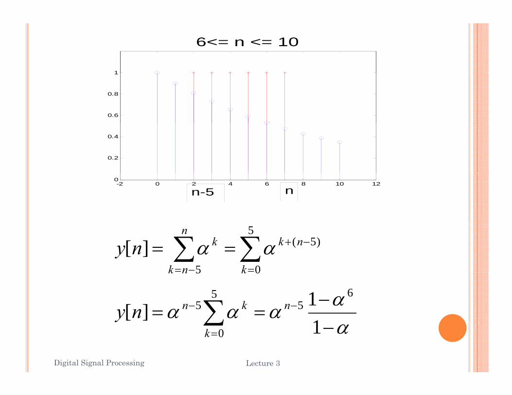
6<= n <= 10
0.6
0.8
1
0.2
0.4
-2 0 2 4 6 8 10 120
n-5 n
∑∑=
−+
−=
==5
0
)5(
5
][k
nkn
nk
kny αα05 knk
αααα −== −− ∑ 1
1][6
55
5 nknny
Digital Signal Processing Lecture 3 11
α−=∑ 10k
y
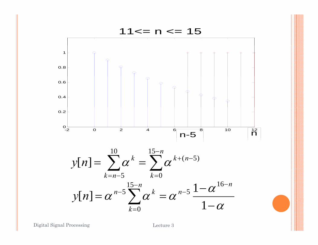
11<= n <= 15
0.8
1
0.4
0.6
-2 0 2 4 6 8 10 120
0.2
n-5 n
∑∑−
−+==n
nkkny15
)5(10
][ αα ∑∑=−= knk 05
αααα −==
−−
−− ∑ 1][
165
155
nn
nknny
Digital Signal Processing Lecture 3 12
α−=∑ 1
][0k
y
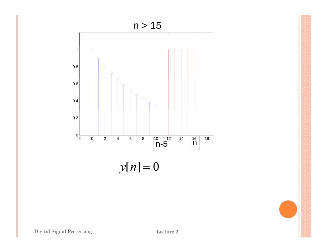
n > 15
0.8
1
0.4
0.6
-2 0 2 4 6 8 10 12 14 16 180
0.2
5 nn-5 n
0][ =ny
Digital Signal Processing Lecture 3 13
Digital Signal Processing Lecture 3 14
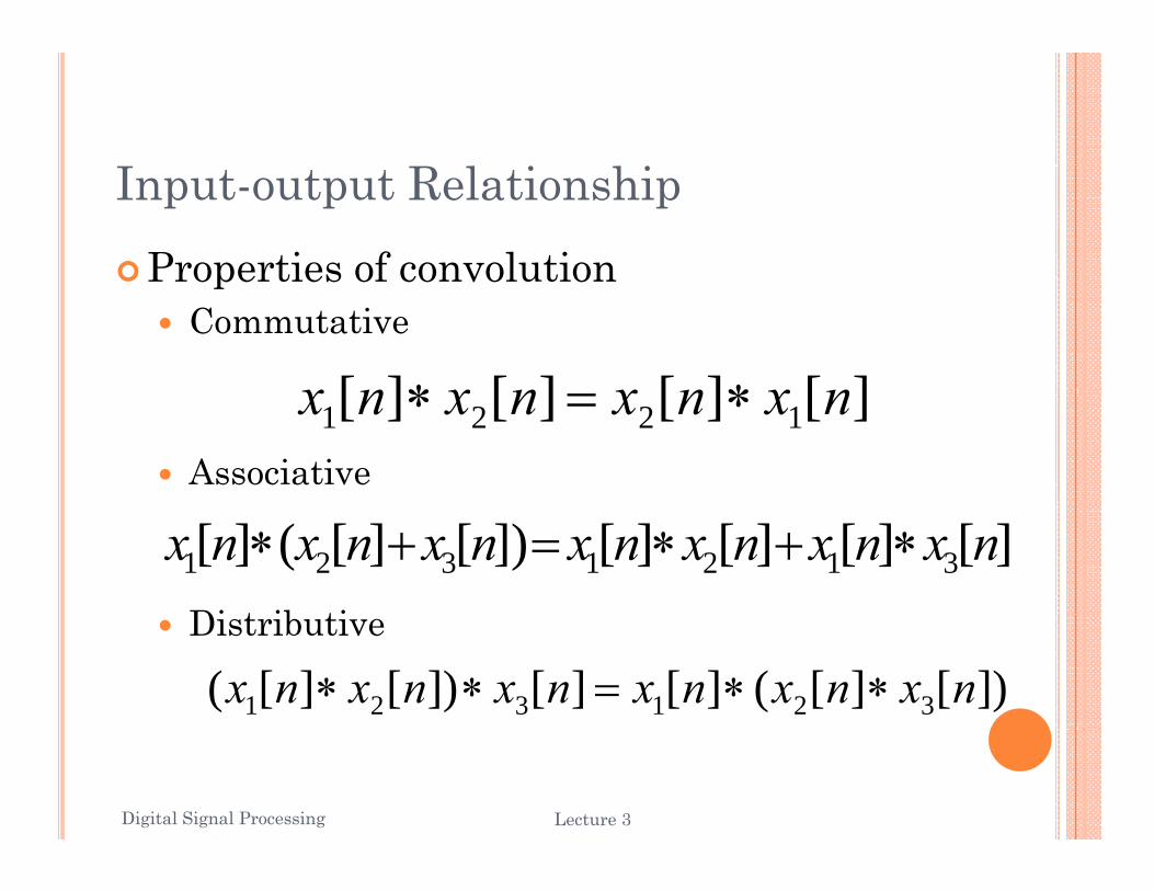
Input-output RelationshipProperties of convolutionProperties of convolution
Commutative
][][][][ nxnxnxnx ∗∗Associative
][][][][ 1221 nxnxnxnx ∗=∗
Di t ib ti
][][][][])[][(][ 3121321 nxnxnxnxnxnxnx ∗+∗=+∗Distributive
])[][(][][])[][( 321321 nxnxnxnxnxnx ∗∗=∗∗
Digital Signal Processing 15Lecture 3
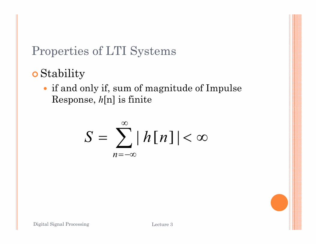
Properties of LTI Systems
StabilityStabilityif and only if, sum of magnitude of Impulse Response, h[n] is finite
∞<= ∑∞
nhS |][| ∞<= ∑−∞=n
nhS |][|
Digital Signal Processing 16Lecture 3
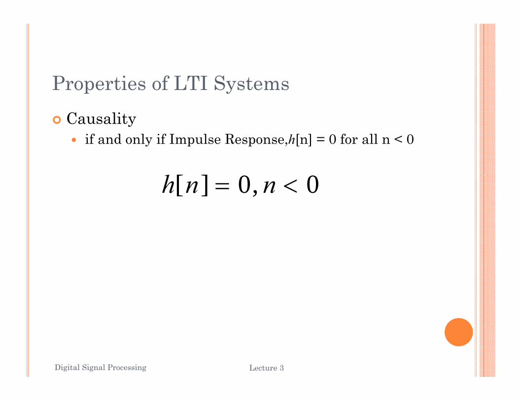
Properties of LTI SystemsCausalityy
if and only if Impulse Response,h[n] = 0 for all n < 0
h 0,0][ <= nnh
Digital Signal Processing 17Lecture 3
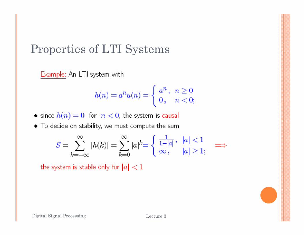
Properties of LTI Systems
Digital Signal Processing 18Lecture 3
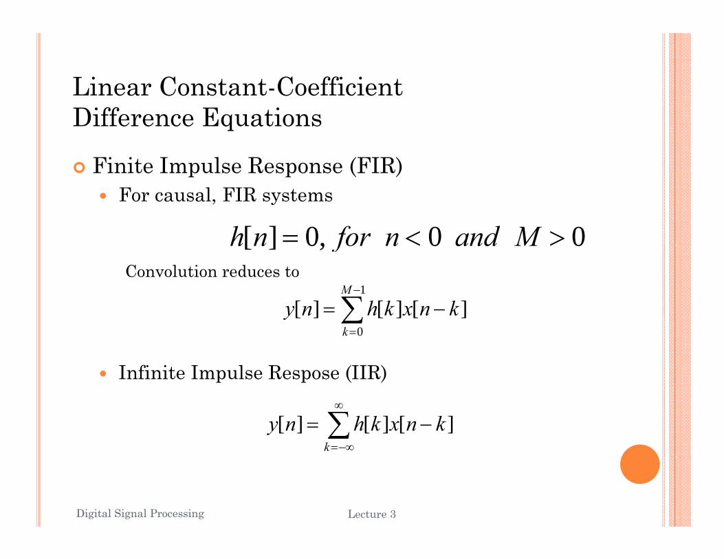
Linear Constant-Coefficient Difference Equations
Finite Impulse Response (FIR)p p ( )For causal, FIR systems
00,0][ ><= MandnfornhConvolution reduces to
0 0 ,0][ >< Mandnfornh
∑−
−=1
][][][M
knxkhny
Infinite Impulse Respose (IIR)
∑=0
][][][k
knxkhny
∑∞
−∞=
−=k
knxkhny ][][][
Digital Signal Processing 19Lecture 3
Linear Constant-Coefficient Difference Equations
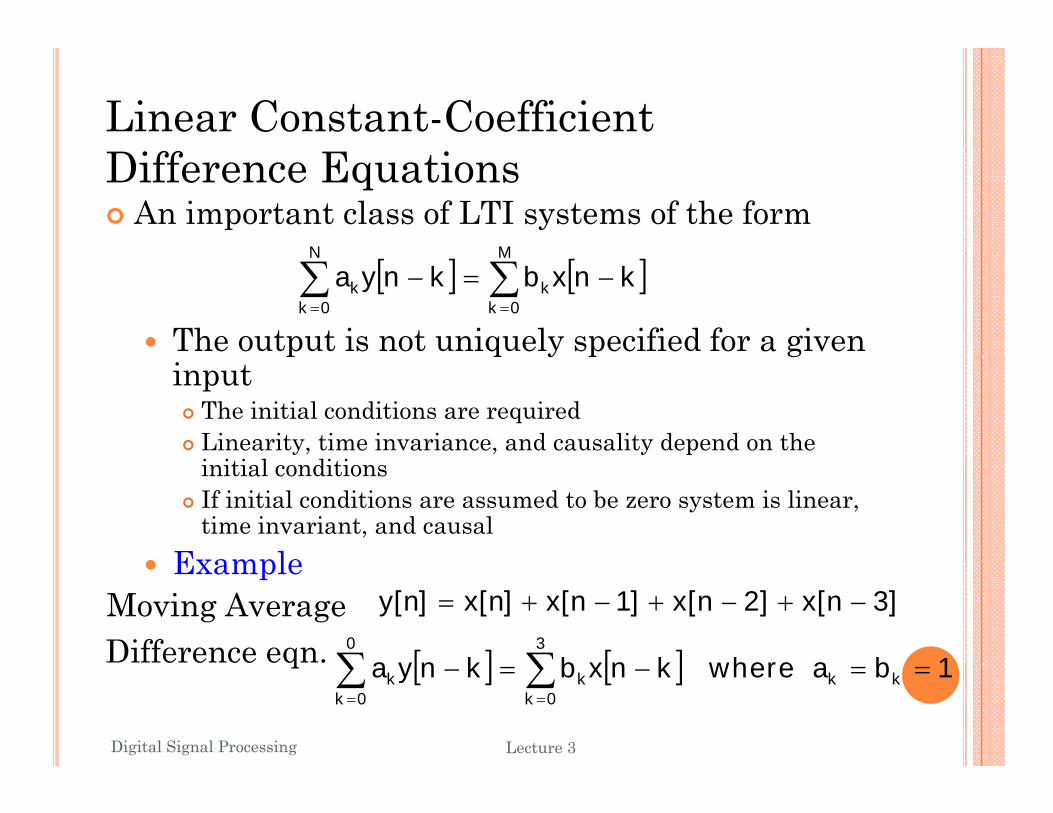
An important class of LTI systems of the formMN
The output is not uniquely specified for a given
[ ] [ ]∑∑==
−=−M
0kk
N
0kk knxbknya
p q y p ginput
The initial conditions are requiredLinearity, time invariance, and causality depend on the initial conditionsIf initial conditions are assumed to be zero system is linear, time invariant, and causal
ExampleExampleMoving AverageDifference eqn.
]3n[x]2n[x]1n[x]n[x]n[y −+−+−+=
[ ] [ ] 1ba where knxbknya30
∑∑q
Digital Signal Processing 20Lecture 3
[ ] [ ] 1ba where knxbknya kk0k
k0k
k ==−=− ∑∑==
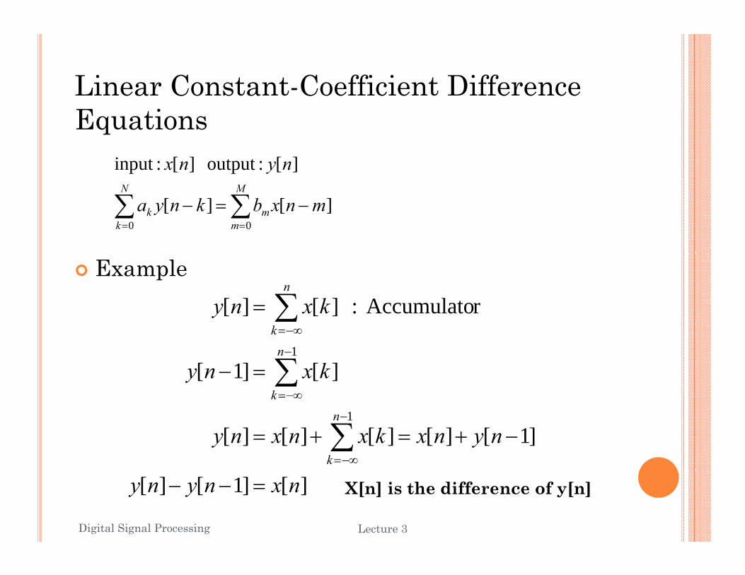
Linear Constant-Coefficient Difference Equations
nynx ][:output ][ :input
∑ ∑= =
−=−N
k
M
mmk mnxbknya
0 0][][
ExamplerAccumulato : ][][ kxny
n
= ∑
][]1[1
kxnyn
k
k
=− ∑−
−∞=
−∞=
]1[][][][][1
nynxkxnxnyn
k
k
−+=+= ∑−
−∞=
∞=
Digital Signal Processing 21Lecture 3
][]1[][ nxnyny =−− X[n] is the difference of y[n]
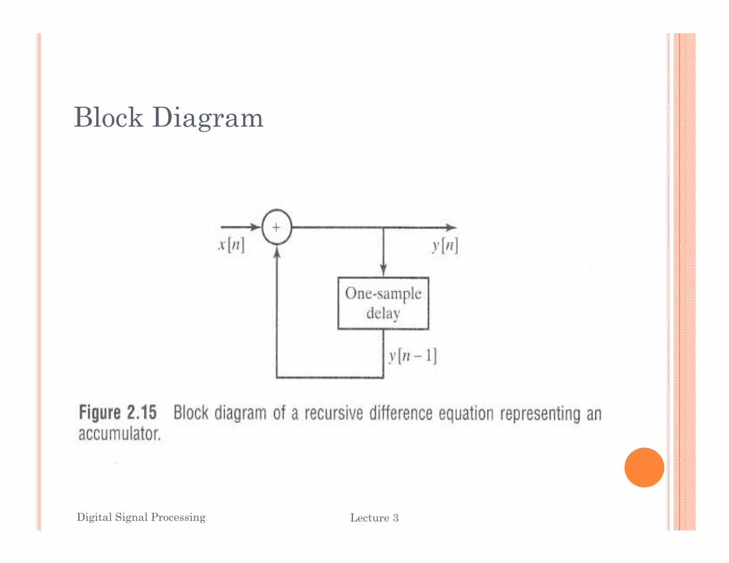
Block Diagram
Digital Signal Processing 22Lecture 3
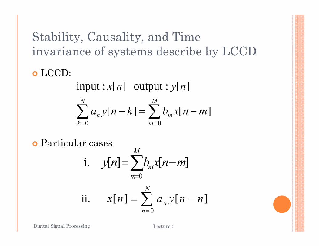
Stability, Causality, and Time invariance of systems describe by LCCD
LCCD:
∑ ∑N M
bk
nynx
][][
][ :output ][ :input
∑ ∑= =
−=−k m
mk mnxbknya0 0
][][
Particular cases
∑ −=M
m mnxbny ][][ i. ∑=m 0
∑ −=N
nnyanx ][][ii
Digital Signal Processing 23Lecture 3
∑=n
n nnyanx0
][][ ii.
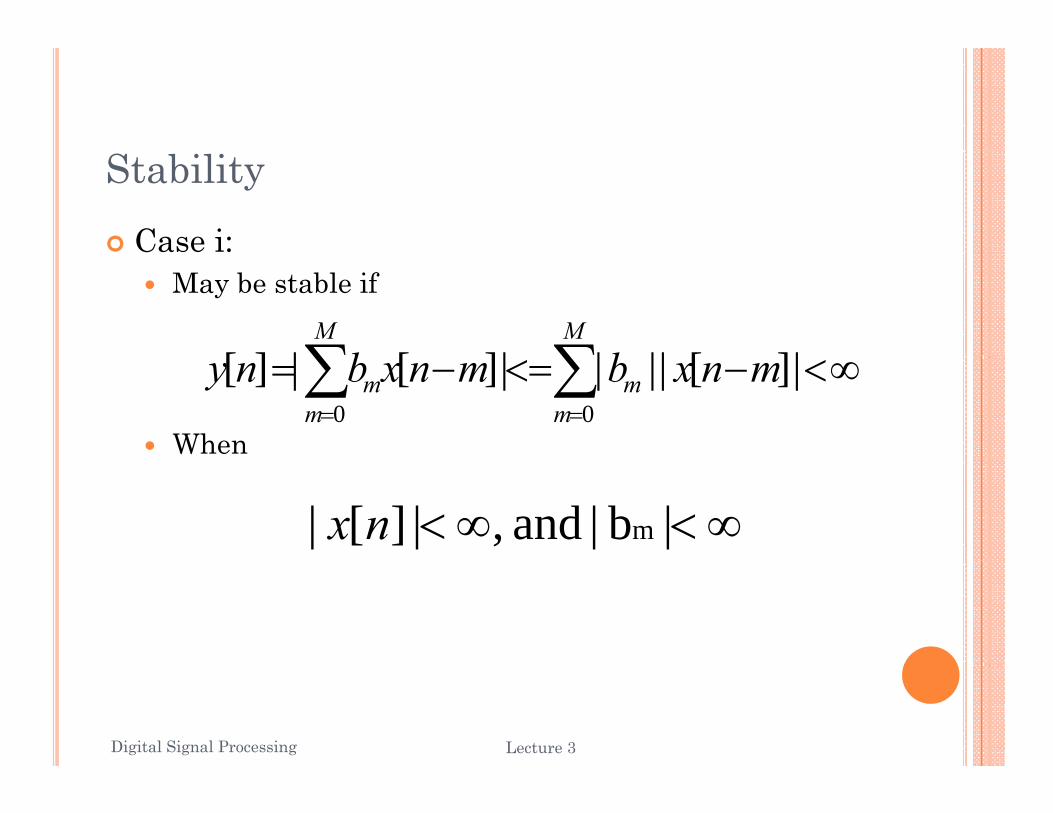
StabilityCase i:
May be stable if
∑∑ |][||||][|][MM
bb
When
∞<−<=−= ∑∑==
|][| |||][|][00 m
mm
m mnxbmnxbny
∞<∞< |b| and ,|][| mnx
Digital Signal Processing 24Lecture 3
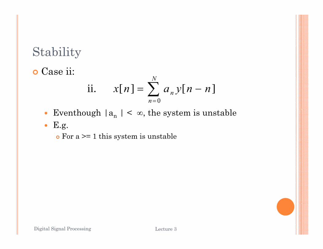
StabilityCase ii:
N
∑=
−=N
nn nnyanx
0][][ ii.
Eventhough |an | < ∞, the system is unstableE.g.
For a >= 1 this system is unstable
Digital Signal Processing 25Lecture 3
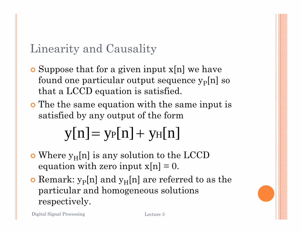
Linearity and CausalitySuppose that for a given input x[n] we have pp g p [ ]found one particular output sequence yP[n] so that a LCCD equation is satisfied.Th th ti ith th i t i The the same equation with the same input is satisfied by any output of the form
[n]y[n]yy[n] +Where yH[n] is any solution to the LCCD
[n]y[n]y y[n] HP +=
equation with zero input x[n] = 0.Remark: yP[n] and yH[n] are referred to as the particular and homogeneous solutions particular and homogeneous solutions respectively.
Digital Signal Processing 26Lecture 3
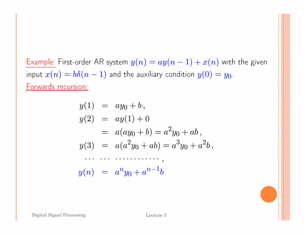
Linearity and CausalityA LCCD equation does not provide a unique q p qspecification of output for a given inputAuxiliary information or conditions are required to specify uniquely the output for a given inputto specify uniquely the output for a given inputExample
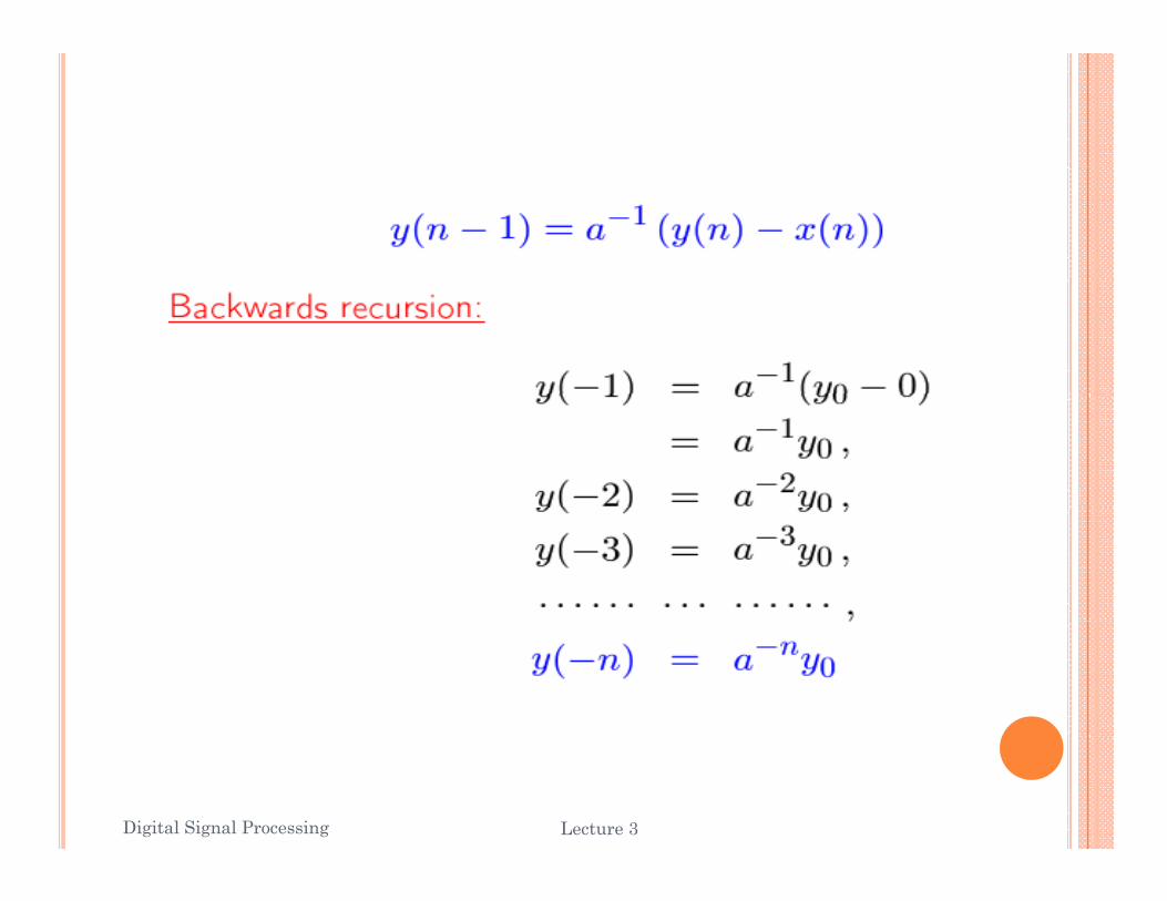
Let auxiliary information be in the form of N sequential output values Thensequential output values. Then,Later values can be obtained by rearranging LCCD equation as a recursive relation running forward in nn.Prior values can be obtained by rearranging LCCD equation as a recursive relation running backward in n.n.
Digital Signal Processing 27Lecture 3
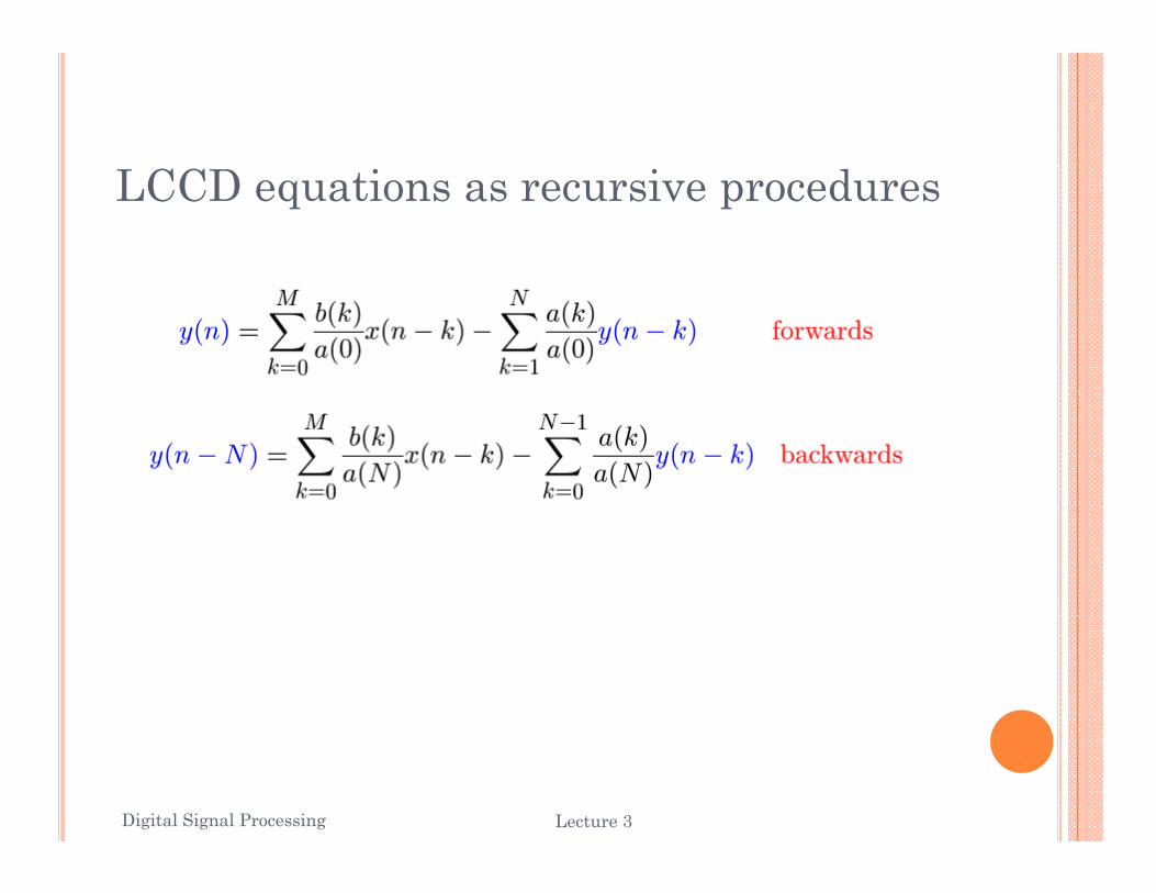
LCCD equations as recursive procedures
Digital Signal Processing 28Lecture 3
Digital Signal Processing Lecture 3 29
Digital Signal Processing Lecture 3 30
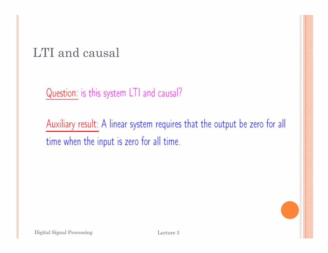
LTI and causal
Digital Signal Processing 31Lecture 3
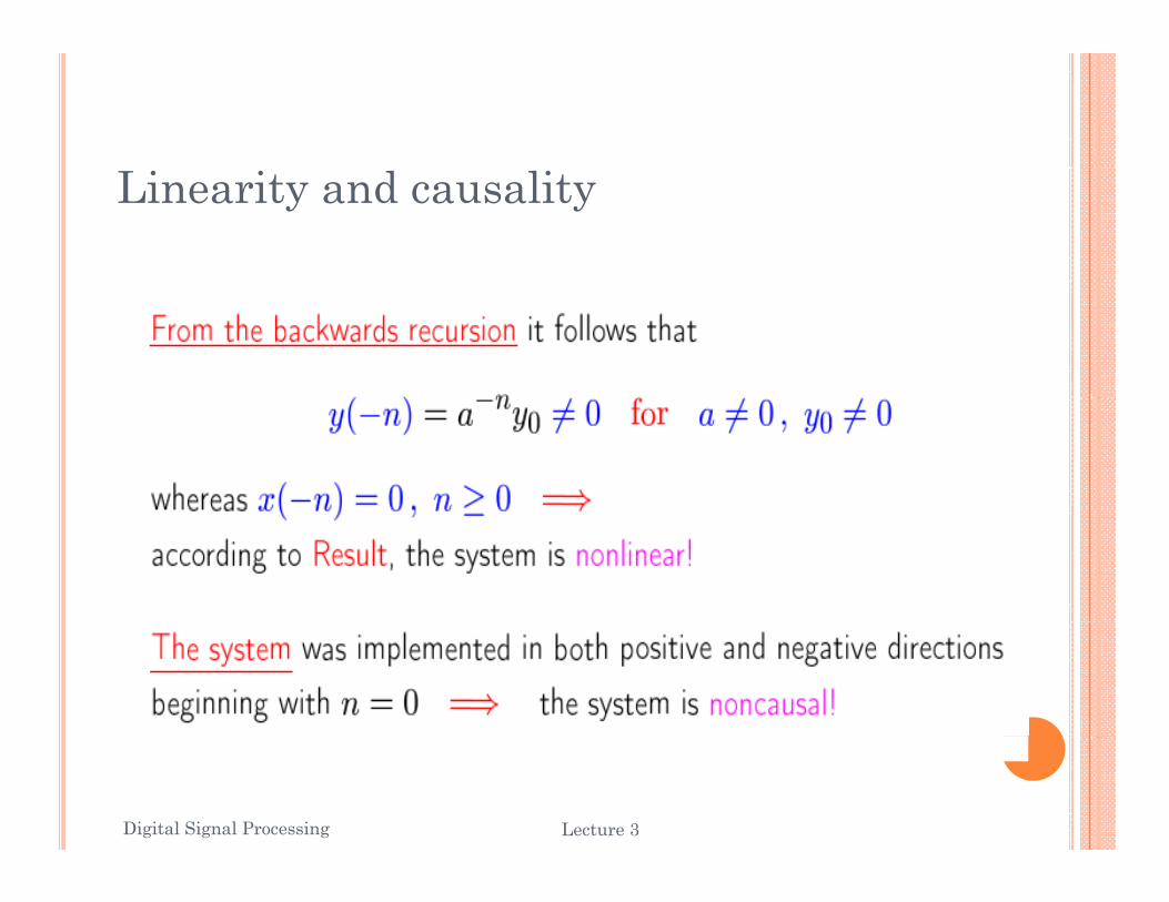
Linearity and causality
Digital Signal Processing 32Lecture 3
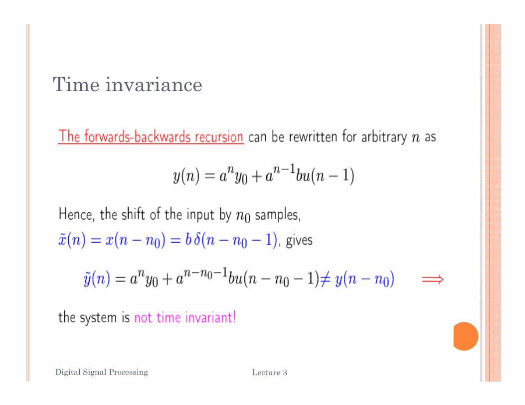
Time invariance
Digital Signal Processing 33Lecture 3
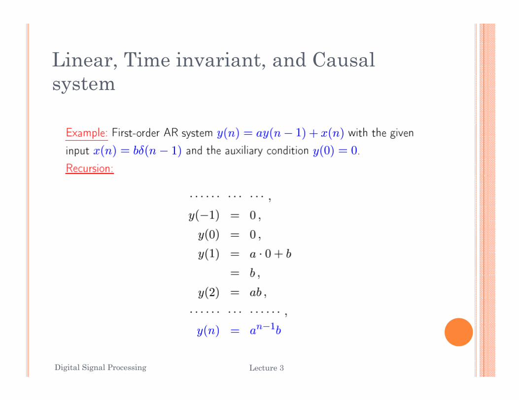
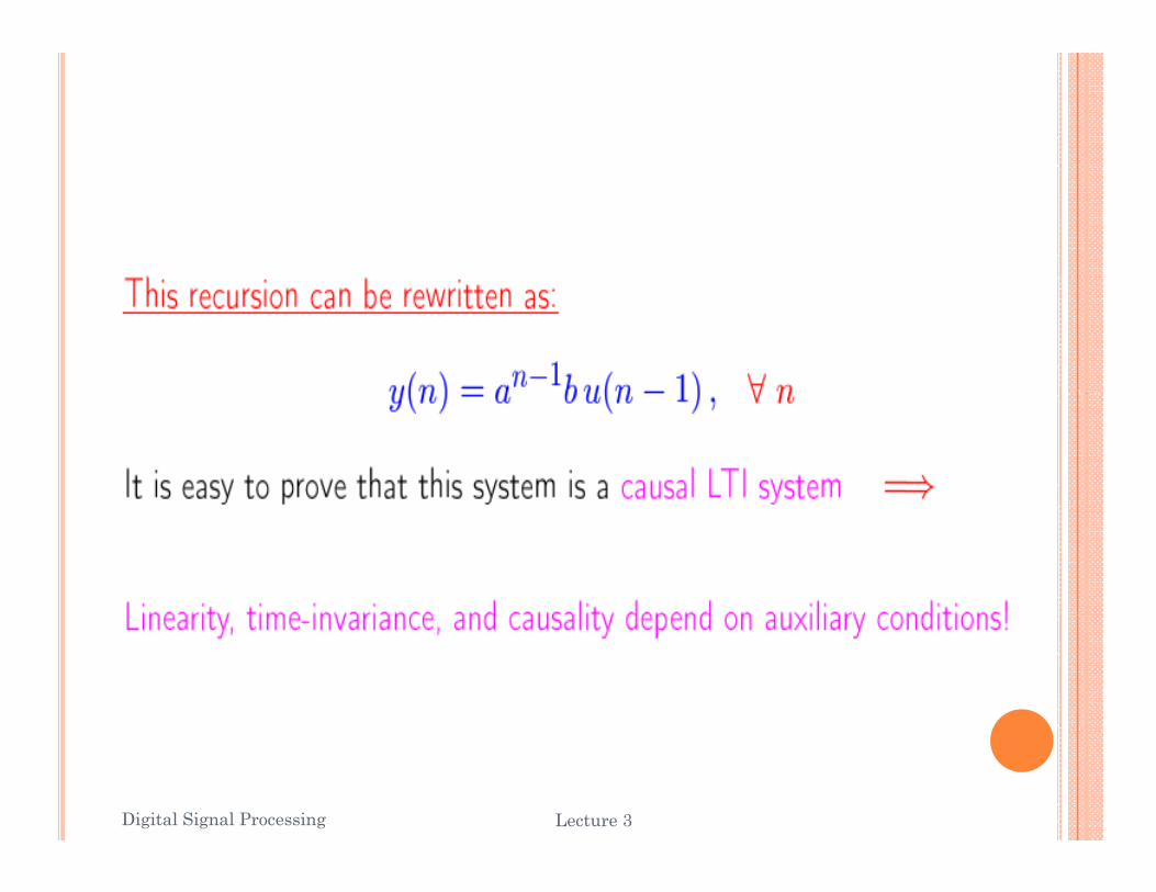
Linear, Time invariant, and Causal system
Digital Signal Processing 34Lecture 3
Digital Signal Processing Lecture 3 35