ASHםיהולא ולש ןגב ןדעה לכ הז םג םע לועהם

λλ λ

λ

λλ

Digital Circuits in CλaSH

Functional Speciications and Type-Directed Synthesis

Christiaan P.R. Baaij

Digital Circuits in CλaSH

Functional Speciications and Type-Directed Synthesis

Christiaan P.R. Baaij

Members of the dissertation committee:

Prof. dr. ir. G.J.M. Smit University of Twente (promotor)Dr. ir. J. Kuper University of Twente (assistant-promotor)

Prof. dr. J.C. van de Pol University of TwenteProf. dr. ir. B.R.H.M. Haverkort University of TwenteProf. dr. M. Sheeran Chalmers University of Technology

Prof. dr. ir. T. Schrijvers Katholieke Universiteit LeuvenProf. dr. K. Hammond University of St. AndrewsProf. dr. P.M.G. Apers University of Twente (chairman and secretary)

Faculty of Electrical Engineering, Mathematics and Computer Sci-ence, Computer Architecture for Embedded Systems (CAES) group

S(o)OSService-oriented

Operating Systems

his research is conducted within the Service-oriented OperatingSystems (S(o)OS) project (Grant Agreement No. 248465) supportedunder the FP7-ICT-2009.8.1 program of the European Commission.

his research is conducted within the Programming Large ScaleHeterogeneous Infrastructure (Polca) project (Grant AgreementNo.610686) supported under the FP7-ICT-2013.3.4 program of the Eu-ropean Commission.

CTITCTIT Ph.D. thesis Series No. 14-335Centre for Telematics and Information TechnologyUniversity of Twente, P.O. Box 217, NLś7500 AE Enschede

Copyright © 2014 by Christiaan P.R. Baaij, Enschede, he Nether-lands. his work is licensed under the Creative Commons Attribu-tion 4.0 International License. To view a copy of this license, visithttp://creativecommons.org/licenses/by/4.0/.

his thesis was typeset using LATEX2ε , TikZ, and Sublime Text. histhesis was printed by Gildeprint Drukkerijen, he Netherlands.

ISBN 978-90-365-3803-9

ISSN 1381-3617 (CTIT Ph.D. thesis Series No. 14-335)

DOI 10.3990/1.9789036538039

Digital Circuits in CλaSH

Functional Specifications and Type-Directed Synthesis

Proefschrift

ter verkrijging vande graad van doctor aan de Universiteit Twente,

op gezag van de rector magniicus,prof. dr. H. Brinksma,

volgens besluit van het College voor Promotiesin het openbaar te verdedigen

op vrijdag 23 januari 2015 om 14:45 uur

door

Christiaan Pieter Rudolf Baaij

geboren op 1 februari 1985te Leiderdorp

Dit proefschrit is goedgekeurd door:

Prof. dr. ir. G.J.M. Smit (promotor)Dr. ir. J. Kuper (assistent promotor)

Copyright © 2014 Christiaan P.R. BaaijISBN 978-90-365-3803-9

v

Abstract

Over the last three decades, the number of transistors used in microchips has in-creased by three orders of magnitude, from millions to billions. he productivityof the designers, however, lags behind. Designing a chip that uses ever more tran-sistors is complex, but doable, and is achieved by massive replication of function-ality. Managing to implement complex algorithms, while keeping non-functionalproperties, such as area and gate propagation latency, within desired bounds, andthoroughly verifying the design against its speciication, are the main diiculties incircuit design.

It is diicult to measure design productivity quantitatively; transistors per hourwould not be a good measure, as high transistor counts can be achieved by repli-cation. As a motivation for our work we make a qualitative analysis of the toolsavailable to circuit designers. Furthermore, we show how these tools manage thecomplexity, and hence improve productivity. Here we see that progress has beenslow, and that the same techniques have been used for over 20 years. Industrystandard languages, such as VHDL and (System)Verilog, do provide means forabstractions, but they are distributed over separate language constructs and havead hoc limitations. What is desired is a single abstraction mechanism that cancapture most, if not all, common design patterns. Once we can abstract our com-mon patterns, we can reason about them with rigour. Rigorous analysis enables usto develop correct-by-construction transformations that capture trade-ofs in thenon-functional properties. hese correct-by-construction transformations give usa straightforward path to reaching the desired bounds on non-functional properties,while signiicantly reducing the veriication burden.

We claim that functional languages can be used to raise the abstraction level incircuit design. Especially higher-order functional languages, where functions areirst-class and can be manipulated by other functions, ofer a single abstractionmechanism that can capture many design patterns. An additional property offunctional languages that make them a good candidate for circuit design is purity,which means that functions have no side-efects. When functions are pure, wecan reason about their composition and decomposition locally, thus enabling usto reason formally about transformations on these functions. Without side-efects,synthesis can derive highly parallel circuits from a functional description becauseit only has to respect the direct data dependencies.

In existing work, the functional language Haskell has been used as a host for em-bedded hardware description languages. An embedded language is actually a set of

vidata types and expressions described within the host language. hese data typesand expressions then act like the keywords of the embedded language. Functionsin the host language are subsequently used to model functions in the embeddedlanguage. Althoughmany features of the host language can be used to model equiv-alent behaviour in the embedded language, this is not true for all features. One ofthe most important features of the host language that cannot directly be used inthe embedded language, are features that model choice, such as pattern matching.

his thesis explores the idea of using the functional language Haskell directly as ahardware speciication language, and move beyond the limitations of embeddedlanguages. Additionally, where applicable, we can use normal functions from exist-ing Haskell libraries to model the behaviour of our circuits.

here are multiple ways to interpret a function as a circuit description. his thesismakes the choice of interpreting a function deinition as a structural composition ofcomponents. his means that every function application is interpreted as the com-ponent instantiation of the respective sub-circuit. Combinational circuits are thendescribed as functions manipulating algebraic data types. Synchronous sequentialcircuits are described as functions manipulating ininite streams of values. In orderto reduce the cognitive burden, and to guarantee synthesisable results, streams can-not be manipulated directly by the designer. Instead, our system ofers a limitedset of combinators that can safely manipulate streams, including combinators thatmap combinational functions over streams. Additionally, the system ofers streamsthat are explicitly synchronised to a particular clock and thus enable the design ofmulti-clock circuits. Proper synchronisation between clock domains is checked bythe type system.

his thesis describes the inner workings of our CλaSH compiler, which translatesthe aforementioned circuit descriptions written in Haskell to low-level descriptionsin VHDL. Because the compiler uses Haskell directly as a speciication language,synthesis of the description is based on (classic) static analysis. he challenge thenbecomes the reduction of the higher-level abstractions in the descriptions to a formwhere synthesis is feasible. his thesis describes a term rewrite system (with boundvariables) to achieve this reduction. We prove that this term rewrite system alwaysreduces a polymorphic, higher-order circuit description to a synthesisable variant.he only restriction is that the root of the function hierarchy is not polymorphicnor higher-order. here are, however, no restrictions on the use of polymorphismand higher-order functionality in the rest of the function hierarchy.

Even when descriptions use high-level abstractions, the CλaSH compiler can syn-thesize eicient circuits. Case studies show that circuits designed in Haskell, andsynthesized with the CλaSH compiler, are on par with hand-written VHDL, in botharea and gate propagation delay. Even in the presence of contemporary Haskell id-ioms and abstractions to write imperative code (for a control-oriented circuit),does the CλaSH compiler create results with decent non-functional properties.To emphasize that our approach enables correct-by-construction descriptions, wedemonstrate abstractions that allow us to automatically compose components that

viiuse back-pressure as their synchronisation method. Additionally, we show howcycle delays can be encoded in the type-signatures of components, allowing us tocatch any synchronisation error at compile-time.

his thesis thus shows the merits of using a modern functional language for circuitdesign. he advanced type system and higher-order functions allow us to designcircuits that have the desired property of being correct-by-construction. Finally,our synthesis approach enables us to derive eicient circuits from descriptions thatuse high-level abstractions.

viii

ix

Samenvatting

Gedurende de laatste drie decennia is het aantal transistors in een processor metdrie ordegroottes toegenomen, van miljoenen naar miljarden. De productiviteitvan de ontwerpers loopt hier echter op achter. Het ontwerpen van een processormet telkens meer transistors is complex, maar doenlijk, en wordt bereikt door hetveelvuldig kopiëren van functionaliteit. Het implementeren van complexe algorit-mes, en het daarbij in toom houden van niet-functionele aspecten, zoals opper-vlakte en propagatievertraging, en het zorgvuldig veriiëren van het uiteindelijkeontwerp, zijn de voornaamste moeilijkheden in het ontwerpen van digitale circuits.

Het is moeilijk om productiviteit van ontwerpers kwantitatief te bepalen; transis-tors per uur is geen goede maat, omdat hoge transistoraantallen kunnen wordenbereikt door replicatie van functionaliteit. Als motivatie voor ons werk maken weeen kwalitatieve analyse van de sotware die beschikbaar is voor ontwerpers vandigitale circuits. Hierbij laten we zien hoe deze sotware helpt bij het beheersenvan de complexiteit en dus de productiviteit verhoogt. We zien dan een geringevoortgang, waarbij dezelfde technieken al meer dan 20 jaar worden gebruikt. Talendie de standaard zijn in de industrie, zoals VHDL en (System)Verilog, verschafenwel abstractiemogelijkheden, maar deze zijn verspreid over verschillende delen vande taal en hebben ad hoc beperkingen. Het is wenselijk om één abstractiemecha-nisme te hebben waarmee we veel, dan niet alle, ontwerppatronen kunnen uitdruk-ken. Wanneer we onze ontwerppatronen kunnen abstraheren, kunnen we er ookgrondig over redeneren. Grondige analyses staan ons toe om inherent correctetransformaties te ontwerpen die afwegingen van niet-functionele eigenschappenuitdrukken. Omdat deze transformaties inherent correct zijn, is het mogelijk omtot een ontwerp te komenmet de gewenste niet-functionele eigenschappen, zonderdat we extra veriicatiestappen hoeven te ondernemen.

Wij beweren dat functionele talen zeer geschikt zijn om het abstractieniveau, vanhet ontwerpen van digitale circuits, naar een hoger niveau te tillen. Zeker hogere-orde functies, waar functies andere functies kunnen bewerken, zijn geschikt alsenkel abstractiemechanisme voor vele ontwerppatronen. Een andere eigenschapvan functionele talen die ze geschikt maakt voor het ontwerpen van digitale circuitsis dat functies vrij zijn van nevenefecten. Omdat functies geen nevenefecten heb-ben kunnenwe op lokaal niveau redeneren over de compositie en decompositie vanfuncties, en zodanig ook formeel redeneren over transformaties van deze functies.Vrij van nevenefecten, kan het syntheseproces zeer parallelle circuits aleiden vanzo’n functionele beschrijving, omdat er alleen rekening gehouden hoet te wordenmet directe afhankelijkheden.

xIn bestaand werk is er gekeken naar het gebruik van de functionele taal Haskellals kadertaal voor ingebedde hardwarebeschrijvingstalen. Zo’n ingebedde taal iseigenlijk een verzameling van datatypes en functies beschreven in de kadertaal,waar deze functies en datatypes dienen als trefwoorden van de ingebedde taal.Alhoewel vele aspecten van de kadertaal gebruikt kunnen worden om equivalenteaspecten in de ingebedde taal uit te drukken, geldt dat niet zo voor alle aspectenvan de kadertaal. Eén van de belangrijkste aspecten van de kadertaal die niet in deingebedde taal gebruikt kanworden, zijn de aspecten die keuze uit kunnen drukken,zoals patroonherkenning.

Dit proefschrit verkent het idee om de functionele taal Haskell direct als hardwa-resbeschrijvingstaal te gebruiken, zodat we niet meer onderhevig hoeven te zijnaan de beperkingen van ingebedde talen. Daarbij is het dan ook mogelijk, waardat van toepassing is, om direct functies uit de standaardbibliotheken te gebruikenvoor het beschrijven van digitale circuits.

Er zijn meerdere manieren om een functie als digitaal circuit te interpreteren. Indit proefschrit kiezen wij ervoor om functies te interpreteren als een structurelecompositie van componenten. Dit betekent dat elke toegepaste functie wordt geïn-terpreteerd als een nieuwe instantie van het overeenkomstige circuit. Combinatori-sche circuits worden beschreven als functies die algebraïsche datatypes bewerken.Synchroon sequentiële circuits worden beschreven als functies die oneindig langereeksen van waarden bewerken. Om de cognitieve last te verlichten, en om synthe-tiseerbare resultaten te garanderen, kunnen zulke oneindige reeksen van waardenniet direct bewerkt kunnen worden de ontwerper. In plaats daarvan biedt het sys-teem een beperkte set van functies die de ontwerper toe staan de reeks op eenbepaalde manier te bewerken, zoals een functie die elementsgewijs een combinato-rische functie toepast op de reeks van waarden. Daarbij zijn er reeksen die explicietzijn gekoppeld aan een speciieke klok, welk het mogelijk maakt om circuits teontwerpen met meerdere klokken. Correcte overgangen tussen de klokdomeinenworden gecontroleerd door het typesysteem.

Dit proefschrit beschrijt de interne werking van de CλaSH compiler, welk eerder-genoemde circuitbeschrijvingen in Haskell omzet naar laag-niveau beschrijvingeninVHDL.Omdat de compilerHaskell direct als speciicatietaal gebruikt, is synthesegebaseerd op (klassieke) statische analyse. De uitdaging zit dan in het reducerenvan de hoog-niveau abstractiemechanismen die zich bevinden in de beschrijvingennaar een vorm waar synthese doenlijk is. Dit proefschrit beschrijt een termher-schrijfsysteem (met gebonden variabelen) om deze reductie te bereiken. We bewij-zen dat dit termherschrijfsysteem altijd polymorfe hogere-orde beschrijvingen vancircuits reduceert naar een synthetiseerbare variant. De enige beperking is dat defunctie bovenaan in de functiehiërarchie niet polymorf noch van hogere-orde is.Er zijn echter geen beperkingen in de rest van die functiehiërarchie wat betret hetgebruik van polymorisme en hogere-orde functionaliteit.

Zelfs wanneer de beschrijvingen abstracties van een hoog niveau bevatten is deCλaSH compiler in staat hiervan eiciënte circuits te synthetiseren. Casestudies

xilaten zien dat circuits die zijn ontworpen in Haskell, en gesynthetiseerd zijn metCλaSH, gelijkwaardig zijn aan circuits direct ontworpen in VHDL, zowel in grootteals in propagatievertraging. Ook wanneer eigentijdse Haskell idiomen wordengebruikt om imperatieve code (voor een controlegeoriënteerd circuit) te schrij-ven is de CλaSH compiler in staat om resultaten te genereren met degelijke niet-functionele aspecten. Om te benadrukken dat onze aanpak de gelegenheid geetom inherent correcte beschrijvingen te ontwerpen, demonstreren wij abstractiesdie het mogelijk maken om circuits met elkaar te verbinden die tegendruk gebrui-ken als synchronisatiemethode. Ook laten we zien hoe klokslagvertragingen aande typesignaturen van componenten kunnen worden toegevoegd, zodat we incor-recte synchronisatie tussen componenten al kunnen afvangen op het moment vanontwerpen.

Dit proefschrit laat dus zien waarom een moderne functionele taal zeer geschiktis voor het ontwerpen van digitale circuits. Het geavanceerde typesysteem en dehogere-orde functies maken het mogelijk om ontwerpen te maken die inherentcorrect zijn. Tenslotte zorgt onze syntheseaanpak ervoor dat we eiciënte circuitskunnen aleiden van beschrijvingenwelke abstracties van een hoog niveau bevatten.

xii

xiii

Dankwoord

November 2008, ik was op zoek naar een masteropdracht, januari 2015, ik ga pro-moveren. Zes jaar lang gewerkt aan hetzelfde onderwerp, waarvan het laatste jaarvoornamelijk aan dit boekje. Ondertussen werken er al meerdere mensen, zelfs vanbuiten de vakgroep, met de sotware die er is geschreven, iets waar ik zeer tevredenover ben. Ook al geloof je in je eigen verhaal, geet het toch een grote voldoeningwanneer ook andere mensen jouw werk nuttig en interessant vinden.

Gedurende deze reis van zes jaar zijn er vele mensen die mij hebben geholpen metmijn werk, en nog belangrijker, ze hebben er voor gezorgd dat ik het altijd naarmijn zin heb gehad. Daarvoor wil ik hun graag bedanken.

Jan, voor de introductie tot de beste manier van programmeren, maar ook onzeplezierige en uitgebreide discussies tijdens de reizen door heel Europa. Bij de eersteprojectvergaderingen van SoOS had ik echt het gevoel alsof we daar niks haddengedaan, maar daar wist jij dan altijd wel weer een positieve draai aan te geven. Nuweet ik inmiddels dat niet alles in twee dagen geregeld kan worden. Gerard, voorhet zorgen voor een plek waar ik de kans kreeg om onderzoek te doen wat ik leukvind, en, wat toch zeker heet bijgedragen dat ik wilde gaan promoveren, dat je eengroep hebt gecreëerd waar ik me als masterstudent volwaardig lid van de groepvoelde.

Koen, een goed klankboord voor al jouw continue wiskunde problemen was iknooit, maar het is wel altijd gezellig met jou op de kamer. Of je nu zelfs een gevatteopmerking maakt, of onbedoeld een opmerking maakt waar iemand anders eengevat weerwoord op heet, zorg je altijd voor veel humor op de groep. Arjan enPhilip, voor het helpen bij het oplossen van problemen van een zekere functioneleaard. Gerald, voor de eerste verkenning van tijdsannotaties op de functionele be-schrijvingen. Rinse, Peter, Ruud, Jaco, Erwin, hoewel de compiler natuurlijk altijdwel werkte op mijn computer met mijn voorbeelden, ben ik toch blij met de veletestcode en bugreports die door jullie zijn geleverd. Jochem, voor de interessantediscussies over bitcoin en andere politieke en inanciële wereldzaken. Marlous,helma, en Nicole, voor het regelen van hotels, vliegreizen, en nog zo vele anderezaken. Marloes voor een gezellige afsluiting van de dag wanneer we samen naarhuis ietsen. Karel en Tom, voor de mooie gesprekken tijdens pauzes, borrels, enonder het gamen, en natuurlijk onze gedeelde waardering voor ilms met een hoogTSH¹ gehalte.

1Deze zal je niet terugvinden in de acronymenlijst.

xivTenslotte, mijn geliefde Alexandra, voor het geduldig aanhoren als ik je terloopsvertel dat ik de volgende dag voor eenweekweg ben voor conferentie, voor het vrien-delijk herinneren dat de buren ook mijn geram op de toetsenbordplank kunnenhoren, en het me bijstaan in vele achtereenvolgende weekenden toen ik doorwerkteaan dit boekje.

ChristiaanEnschede, december 2014

xv

Contents

1 Introduction 1

1.1 Hardware Description Languages . . . . . . . . . . . . . . . . . . 3

1.2 Functional Hardware Description Languages . . . . . . . . . . . 61.2.1 Sequential logic . . . . . . . . . . . . . . . . . . . . . . . . . 71.2.2 Higher level abstractions . . . . . . . . . . . . . . . . . . . . . 91.2.3 Challenges in synthesising functional HDLs to circuits . . . . . 10

1.3 Research questions . . . . . . . . . . . . . . . . . . . . . . . . . . . 11

1.4 Approach and contributions of the thesis . . . . . . . . . . . . . . 11

1.5 Structure of the thesis . . . . . . . . . . . . . . . . . . . . . . . . . 13

2 Hardware Description Languages 15

2.1 Introduction . . . . . . . . . . . . . . . . . . . . . . . . . . . . . . 15

2.2 Standard hardware description languages . . . . . . . . . . . . . . 162.2.1 VHDL . . . . . . . . . . . . . . . . . . . . . . . . . . . . . . 162.2.2 Verilog . . . . . . . . . . . . . . . . . . . . . . . . . . . . . . 182.2.3 SystemVerilog . . . . . . . . . . . . . . . . . . . . . . . . . . 192.2.4 BlueSpec SystemVerilog . . . . . . . . . . . . . . . . . . . . . 20

2.3 Functional Languages . . . . . . . . . . . . . . . . . . . . . . . . . 212.3.1 Conventional Languages . . . . . . . . . . . . . . . . . . . . . 212.3.2 Embedded Languages . . . . . . . . . . . . . . . . . . . . . . 26

2.4 Conclusions . . . . . . . . . . . . . . . . . . . . . . . . . . . . . . . 322.4.1 Standard Languages . . . . . . . . . . . . . . . . . . . . . . . 322.4.2 Functional Languages . . . . . . . . . . . . . . . . . . . . . . 33

3 CAES Language for Synchronous Hardware 37

3.1 Introduction . . . . . . . . . . . . . . . . . . . . . . . . . . . . . . 373.1.1 A structural view . . . . . . . . . . . . . . . . . . . . . . . . 38

3.2 Combinational logic . . . . . . . . . . . . . . . . . . . . . . . . . . 393.2.1 Function abstraction and application . . . . . . . . . . . . . . 393.2.2 Types . . . . . . . . . . . . . . . . . . . . . . . . . . . . . . 403.2.3 Choice . . . . . . . . . . . . . . . . . . . . . . . . . . . . . . 42

xvi

Conten

ts

3.3 Higher level abstractions . . . . . . . . . . . . . . . . . . . . . . . 453.3.1 Polymorphism . . . . . . . . . . . . . . . . . . . . . . . . . . 453.3.2 Higher-order functions . . . . . . . . . . . . . . . . . . . . . 48

3.4 Sequential logic . . . . . . . . . . . . . . . . . . . . . . . . . . . . . 523.4.1 Synchronous sequential circuits . . . . . . . . . . . . . . . . . 533.4.2 A safe interface for Signal . . . . . . . . . . . . . . . . . . . . 563.4.3 Abstractions over Signal . . . . . . . . . . . . . . . . . . . . . 583.4.4 Multiple clock domains . . . . . . . . . . . . . . . . . . . . . 61

3.5 Conclusions and future work . . . . . . . . . . . . . . . . . . . . . 663.5.1 Future work . . . . . . . . . . . . . . . . . . . . . . . . . . . 68

4 Type-Directed Synthesis 71

4.1 Introduction . . . . . . . . . . . . . . . . . . . . . . . . . . . . . . 714.1.1 Netlists & Synthesis . . . . . . . . . . . . . . . . . . . . . . . 72

4.2 Compiler pipeline . . . . . . . . . . . . . . . . . . . . . . . . . . . 744.2.1 System FC . . . . . . . . . . . . . . . . . . . . . . . . . . . . 754.2.2 Normal form . . . . . . . . . . . . . . . . . . . . . . . . . . 874.2.3 From normalised System FC to a netlist . . . . . . . . . . . . . 88

4.3 Normalisation . . . . . . . . . . . . . . . . . . . . . . . . . . . . . . 954.3.1 Eliminating non-representable values . . . . . . . . . . . . . . 974.3.2 Completeness of non-representable value removal . . . . . . . . 1054.3.3 Termination of non-representable value removal . . . . . . . . 1154.3.4 Simpliication . . . . . . . . . . . . . . . . . . . . . . . . . . 120

4.4 Discussion . . . . . . . . . . . . . . . . . . . . . . . . . . . . . . . . 1254.4.1 Properties of the normalisation phase . . . . . . . . . . . . . . 1254.4.2 Correspondence operational semantics and netlists . . . . . . . 1264.4.3 Recursive descriptions . . . . . . . . . . . . . . . . . . . . . . 127

4.5 Conclusions . . . . . . . . . . . . . . . . . . . . . . . . . . . . . . . 1284.5.1 Future work . . . . . . . . . . . . . . . . . . . . . . . . . . . 128

5 Advanced aspects of circuit design in CλaSH 135

5.1 Introduction . . . . . . . . . . . . . . . . . . . . . . . . . . . . . . 135

5.2 Streaming reduction circuit . . . . . . . . . . . . . . . . . . . . . . 136

5.3 CλaSH demonstrator circuit . . . . . . . . . . . . . . . . . . . . . 141

5.4 Correct-by-construction compositions . . . . . . . . . . . . . . . 1485.4.1 Back pressure . . . . . . . . . . . . . . . . . . . . . . . . . . 1485.4.2 Delay annotations . . . . . . . . . . . . . . . . . . . . . . . . 154

5.5 Discussion . . . . . . . . . . . . . . . . . . . . . . . . . . . . . . . . 158

xvii

Conten

ts

6 Conclusions 163

6.1 Contributions . . . . . . . . . . . . . . . . . . . . . . . . . . . . . . 165

6.2 Recommendations . . . . . . . . . . . . . . . . . . . . . . . . . . . 165

A First Class Patterns in Kansas Lava 169

B Synchronisation Primitive 173

C System FC 177

D Preservation of the rewrite rules 191

Acronyms 197

Bibliography 199

List of Publications 207

xviii

1

1Introduction

In 1985¹, Intel released the 80386, a consumer-grade central processing unit (CPU)that had around 275.000 transistors. he Intel 80486, released 4 years later, was theirst x86 CPU that crossed the 1 million transistor boundary. he largest availablechip today, in terms of transistor count, is NVIDIA’s GK110 GPU rounding outat about 7 billion transistors. Nearly three decades of technology scaling havethus increased the transistor count by three orders of magnitude: from millions tobillions.

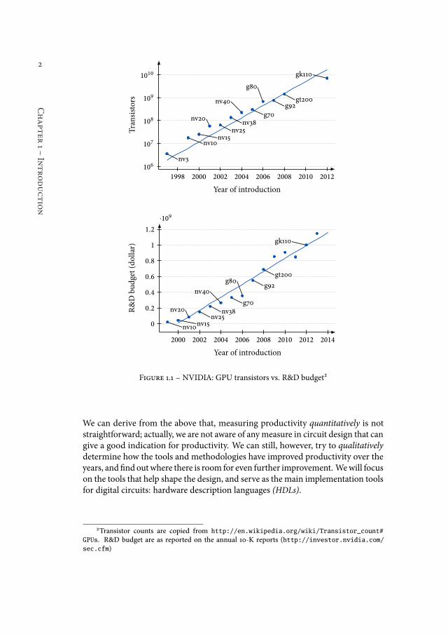
While transistor budgets grew by three orders of magnitude over three decades,it is much harder to determine whether the productivity of chip designer grewequally fast over the years. Figure 1.1 sets out the R&D budget of NVIDIA againstthe transistor count of their GPUs. We choose NVIDIA as their R&D is spenton a small product line, where the main product line is most likely taking up thelargest part of their budget. If we would consider transistors per dollar spent asa measure for productivity, then NVIDIA’s productivity is spectacular: while itsR&D budget grows linearly, the number of transistors used in their GPU grows(almost) exponentially.

Such spectacular productivity growth is of course unlikely; it would have beenwide-spread knowledge within the community if it would be true. Using the number oftransistors as a measure for productivity is not a particularly good measure, thesehigh transistor counts are achieved because GPUs are highly regular. GPUs illtheir transistor budgets through replication: they consist out of hundreds, if notthousands, of identical cores. he same story holds for modern CPUs, for bothmobile and desktop systems: they have multiple cores, sometimes in the doubledigits, and megabytes of cache memory. As replication is straightforward, the realcomplexity of these designs lies with their individual computational units and thecomposition of these units. When we would measure productivity in terms oftransistors used for these individual units, the results are indeed not as spectacular.

1Chosen as a reference as it corresponds to the author’s date of birth.

2

Chapter

1śIntroduction

1998 2000 2002 2004 2006 2008 2010 2012

106

107

108

109

1010

nv3nv3

nv10nv10nv15nv15

nv20nv20

nv25nv25nv38nv38

nv40nv40

g70g70

g80g80

g92g92gt200gt200

gk110gk110

Year of introduction

Transistors

2000 2002 2004 2006 2008 2010 2012 2014

0

0.2

0.4

0.6

0.8

1

1.2

⋅109

nv10nv10nv15nv15

nv20nv20nv25nv25

nv38nv38

nv40nv40

g70g70

g80g80g92g92

gt200gt200

gk110gk110

Year of introduction

R&Dbudget(dollar)

Figure 1.1 ś NVIDIA: GPU transistors vs. R&D budget²

We can derive from the above that, measuring productivity quantitatively is notstraightforward; actually, we are not aware of anymeasure in circuit design that cangive a good indication for productivity. We can still, however, try to qualitativelydetermine how the tools and methodologies have improved productivity over theyears, and ind outwhere there is room for even further improvement. Wewill focuson the tools that help shape the design, and serve as the main implementation toolsfor digital circuits: hardware description languages (HDLs).

2Transistor counts are copied from http://en.wikipedia.org/wiki/Transistor_count#

GPUs. R&D budget are as reported on the annual 10-K reports (http://investor.nvidia.com/sec.cfm)

3

1.1śHardwareDescriptionLanguages

1.1 Hardware Description Languages

he two most commonly used HDLs, VHDL and Verilog, were introduced whenindustry shited circuit design towards very-large-scale integration (VLSI). At thattime, these HDLs were used for the documentation and simulation of circuits thatwere already designed in a diferent format, for example with schematic capturetools. It is the advent of logic synthesis (and automated place & route) that reallypushed VHDL and Verilog to the forefront of digital circuit design. Logic synthesisresulted in an incredible productivity boost compared to schematic capture toolsand the manual layout process that were common practise until that time.

hese logic synthesis tools work on register-transfer level (RTL) descriptions of acircuit. RTL describes a circuit in terms of the composition of the signals betweenregisters, and the logical operations performed on those signals. In order to raisethe abstraction level even further, and hence improve the productivity of circuitdesigner, the next stepwas to just describe the behaviour of the circuit, and derive aneicient structural description [43]. he two well-known approaches to facilitatingbetter behavioural descriptions are:

ż Extending and improving existing HDLs with features from modern pro-gramming languages, such as the object-oriented features of SystemVerilog(an extension, now successor, to Verilog).

ż High-level synthesis (HLS) [13, 43] (or behavioural synthesis) of high level(programming) languages such as C or Java.

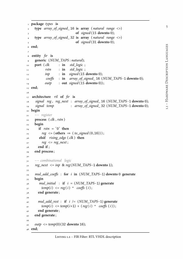
he purpose of high-level synthesis (HLS) is to transform a behavioural, oten se-quential, description of a circuit to an RTL description. HLS is not restricted toregular programming languages, it applies equally to the behavioural feature set ofexisting (and extended) HDLs. he code in listing 1.2 gives an RTL description of ainite impulse response (FIR) ilter in VHDL. It is a fully parallel implementation.here is also one (purposefully included) performance issue: all multiplied valuesare added in a long chain, instead of using a tree of adders, leading to a longercombinational path than necessary.

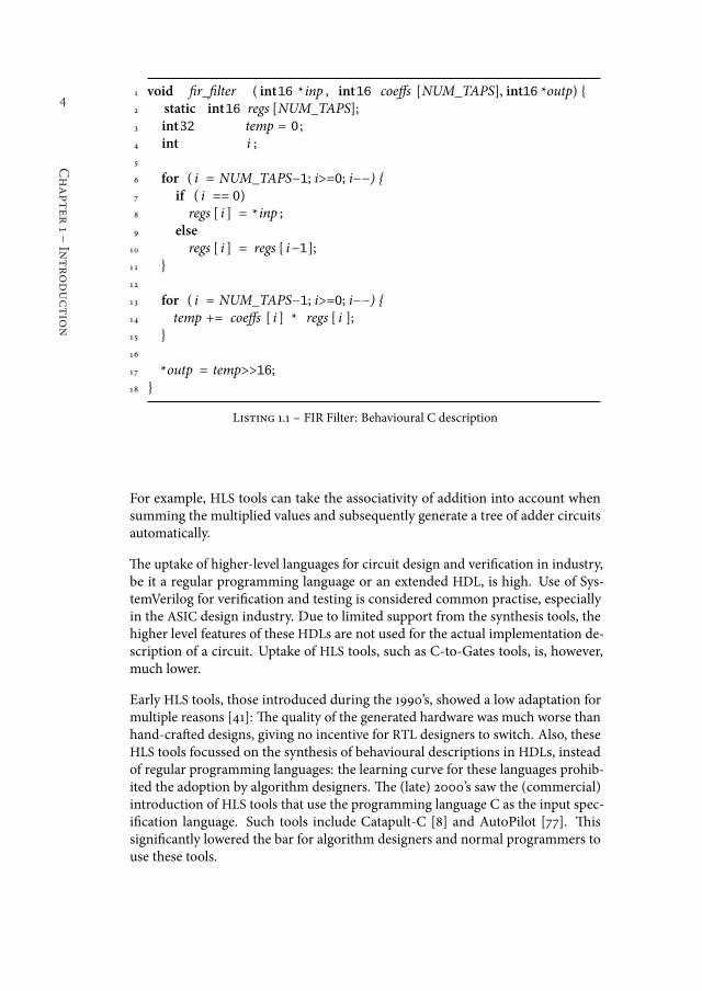
he code in listing 1.1 gives a behavioural description of a FIR ilter inC.hepurposeof a HLS tool is to convert this behavioural description to an RTL description. Itdoes not need to be a fully parallel implementation like the code in listing 1.2 though,it is also possible to map the description to a sequential implementation, one whichcontains only a single multiplier and a single adder. he process for determiningwhether the implementation should be fully parallel, fully sequential, or somethingin between, can either be done:

ż Manually: the HLS tool provides mechanisms to, e.g., unroll and pipelineloops.

ż Automatically: the HLS searches for an implementation that best its thegiven size and latency restrictions.

4

Chapter

1śIntroduction

1 void ir_ilter ( int16 *inp , int16 coefs [NUM_TAPS], int16 *outp) {2 static int16 regs [NUM_TAPS];3 int32 temp = 0 ;4 int i ;5

6 for ( i = NUM_TAPS−1; i>=0; i−−) {7 if ( i == 0)8 regs [ i ] = *inp ;9 else

10 regs [ i ] = regs [ i−1];11 }12

13 for ( i = NUM_TAPS−1; i>=0; i−−) {14 temp += coefs [ i ] * regs [ i ];15 }16

17 *outp = temp>>16;18 }

Listing 1.1 ś FIR Filter: Behavioural C description

For example, HLS tools can take the associativity of addition into account whensumming the multiplied values and subsequently generate a tree of adder circuitsautomatically.

he uptake of higher-level languages for circuit design and veriication in industry,be it a regular programming language or an extended HDL, is high. Use of Sys-temVerilog for veriication and testing is considered common practise, especiallyin the ASIC design industry. Due to limited support from the synthesis tools, thehigher level features of these HDLs are not used for the actual implementation de-scription of a circuit. Uptake of HLS tools, such as C-to-Gates tools, is, however,much lower.

Early HLS tools, those introduced during the 1990’s, showed a low adaptation formultiple reasons [41]: he quality of the generated hardware was much worse thanhand-crated designs, giving no incentive for RTL designers to switch. Also, theseHLS tools focussed on the synthesis of behavioural descriptions in HDLs, insteadof regular programming languages: the learning curve for these languages prohib-ited the adoption by algorithm designers. he (late) 2000’s saw the (commercial)introduction of HLS tools that use the programming language C as the input spec-iication language. Such tools include Catapult-C [8] and AutoPilot [77]. hissigniicantly lowered the bar for algorithm designers and normal programmers touse these tools.

5

1.1śHardwareDescriptionLanguages

1 package types is2 type array_of_signed_ 16 is array ( natural range <>)3 of signed (15 downto 0);4 type array_of_signed_ 32 is array ( natural range <>)5 of signed (31 downto 0);6 end;7

8 entity ir is9 generic (NUM_TAPS : natural);

10 port ( clk : in std_logic ;11 rstn : in std_logic ;12 inp : in signed (15 downto 0);13 coefs : in array_of_signed_ 16 (NUM_TAPS−1 downto 0);14 outp : out signed (15 downto 0));15 end;16

17 architecture rtl of ir is18 signal reg , reg_next : array_of_signed_ 16 (NUM_TAPS−1 downto 0);19 signal temp : array_of_signed_ 32 (NUM_TAPS−1 downto 0);20 begin21 −− register22 process ( clk , rstn )23 begin24 if rstn = ’0 ’ then25 reg <= (others ⇒ ( to_signed (0 ,16))) ;26 elsif rising_edge ( clk ) then27 reg <= reg_next ;28 end if ;29 end process ;30

31 −− combinational logic32 reg_next <= inp & reg (NUM_TAPS−1 downto 1);33

34 mul_add_coefs : for i in (NUM_TAPS−1) downto 0 generate35 begin36 mul_initial : if i = (NUM_TAPS−1) generate37 temp(i ) <= reg ( i ) * coefs ( i ) ;38 end generate ;39

40 mul_add_rest : if i /= (NUM_TAPS−1) generate41 temp(i ) <= temp(i+1) + ( reg ( i ) * coefs ( i ) ) ;42 end generate ;43 end generate ;44

45 outp <= temp(0)(32 downto 16);46 end;

Listing 1.2 ś FIR Filter: RTL VHDL description

6

Chapter

1śIntroduction

Advances in compiler technology, and a focus on the digital signal processing (DSP)parts (instead of the control parts) within circuit designs, has resulted in a muchhigher quality of the hardware that is generated by contemporaryHLS tools [12, 41].hat does not mean that arbitrary C programs can be converted to highly perform-ing circuits: they almost always have to be altered so that the HLS tools can infermore parallelism. Also, although HLS tools are very good at extracting instruction-and loop-level parallelism from C programs, extracting task-level parallelism stillrequires manual annotation [12].

he problems that HLS tools face stems from the sequential, imperative, nature ofthe languages that are used for speciication, and the parallel, immutable, nature ofdigital circuits. Even the most commonly used HDLs are based on languages thatwere created for sequential CPUs: VHDL is based on Ada, and Verilog on C. It thusmakes sense to explore languages that are not created with a sequential platform inmind, and are hopefully better aligned with the parallel nature of digital circuits.

1.2 Functional Hardware Description Languages

he third, lesser travelled and lesser known, road to raising the abstraction level ofcircuit design is to use a programming paradigm that falls outside of the scope ofimperative languages. he most studied, non-imperative, paradigm in the contextof circuit design is functional programming. he tenets of functional programmingare simply function abstraction, the creation of functions, and function application.Two other features oten associated with functional languages are purity and im-mutability, where the two are actually closely related.

Purity is used to indicate that a function always returns the same result for anassociated input; that is, the result is not inluenced by side-efects, nor does afunction produce any side-efects. As mutation is a side-efect, variables in purefunctional languages are immutable. A variable in a functional language is thusakin to a variable in mathematics: a constant, yet unknown, value.

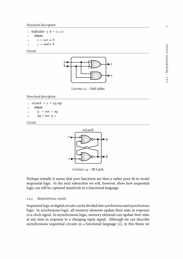
he combinational logic in a digital circuit is a logic function, in the mathematicalsense, from its inputs to its output. he pure functions as those found in func-tional languages embody this function concept of mathematics. Pure functionsare thus a perfect model for the combinational logic in digital circuits. he code inlisting 1.3, describing a half adder circuit, serves as a small example to demonstratethe correspondence between functional descriptions and digital circuits.

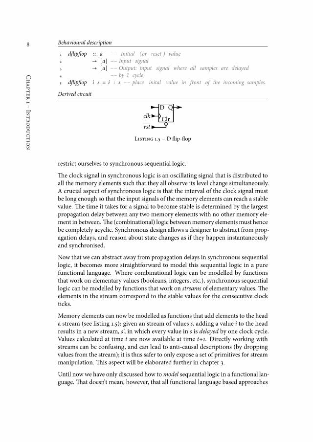
Just like the mathematical function concept they embody, functions in functionallanguages are timeless: there is no notion of time that inluences their behaviour.Circuits on the other hand have propagation delays: it takes time for a level changeto propagate through a circuit. he retention behaviour of memory elements insequential logic crucially depends on these propagation delays. So, although list-ing 1.4 is a good structural description of the combinational logic of an SR latch, thesemantics of the description does not say anything about the propagation delaysand hence the retention behaviour of the SR latch.

7

1.2.1śSequen

tiallo

gic

Structural description

1 halfAdder a b = ( s , c)2 where

3 s = xor a b

4 c = and a b

Circuit

a

bs

c

Listing 1.3 ś Half adder

Structural description

1 srLatch r s = (q ,nq)2 where

3 q = nor r nq

4 nq = nor q s

Circuit

s

rq

q

srLatch

Listing 1.4 ś SR Latch

Perhaps initially it seems that pure functions are thus a rather poor it to modelsequential logic. In the next subsection we will, however, show how sequentiallogic can still be captured intuitively in a functional language.

1.2.1 Sequential logic

Sequential logic in digital circuits can be divided into synchronous and asynchronouslogic. In synchronous logic, all memory elements update their state in responseto a clock signal. In asynchronous logic, memory elements can update their stateat any time in response to a changing input signal. Although we can describeasynchronous sequential circuits in a functional language [2], in this thesis we

8

Chapter

1śIntroduction

Behavioural description

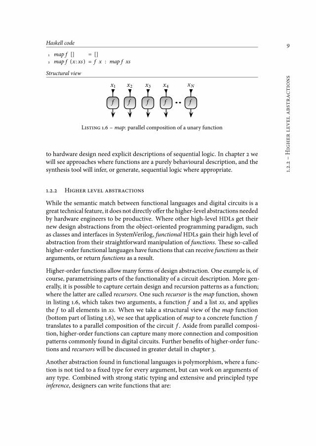
1 dliplop :: a −− Initial (or reset ) value

2 → [a] −− Input signal

3 → [a] −− Output: input signal where all samples are delayed

4 −− by 1 cycle

5 dliplop i s = i : s −− place inital value in front of the incoming samples

Derived circuit

rst

clk

D Q

Clr

Listing 1.5 ś D lip-lop

restrict ourselves to synchronous sequential logic.

he clock signal in synchronous logic is an oscillating signal that is distributed toall the memory elements such that they all observe its level change simultaneously.A crucial aspect of synchronous logic is that the interval of the clock signal mustbe long enough so that the input signals of the memory elements can reach a stablevalue. he time it takes for a signal to become stable is determined by the largestpropagation delay between any two memory elements with no other memory ele-ment in between. he (combinational) logic betweenmemory elementsmust hencebe completely acyclic. Synchronous design allows a designer to abstract from prop-agation delays, and reason about state changes as if they happen instantaneouslyand synchronised.

Now that we can abstract away from propagation delays in synchronous sequentiallogic, it becomes more straightforward to model this sequential logic in a purefunctional language. Where combinational logic can be modelled by functionsthat work on elementary values (booleans, integers, etc.), synchronous sequentiallogic can be modelled by functions that work on streams of elementary values. heelements in the stream correspond to the stable values for the consecutive clockticks.

Memory elements can now be modelled as functions that add elements to the heada stream (see listing 1.5): given an stream of values s, adding a value i to the headresults in a new stream, s’, in which every value in s is delayed by one clock cycle.Values calculated at time t are now available at time t+1. Directly working withstreams can be confusing, and can lead to anti-causal descriptions (by droppingvalues from the stream); it is thus safer to only expose a set of primitives for streammanipulation. his aspect will be elaborated further in chapter 3.

Until now we have only discussed how tomodel sequential logic in a functional lan-guage. hat doesn’t mean, however, that all functional language based approaches

9

1.2.2śHigher

levelabstractions

Haskell code

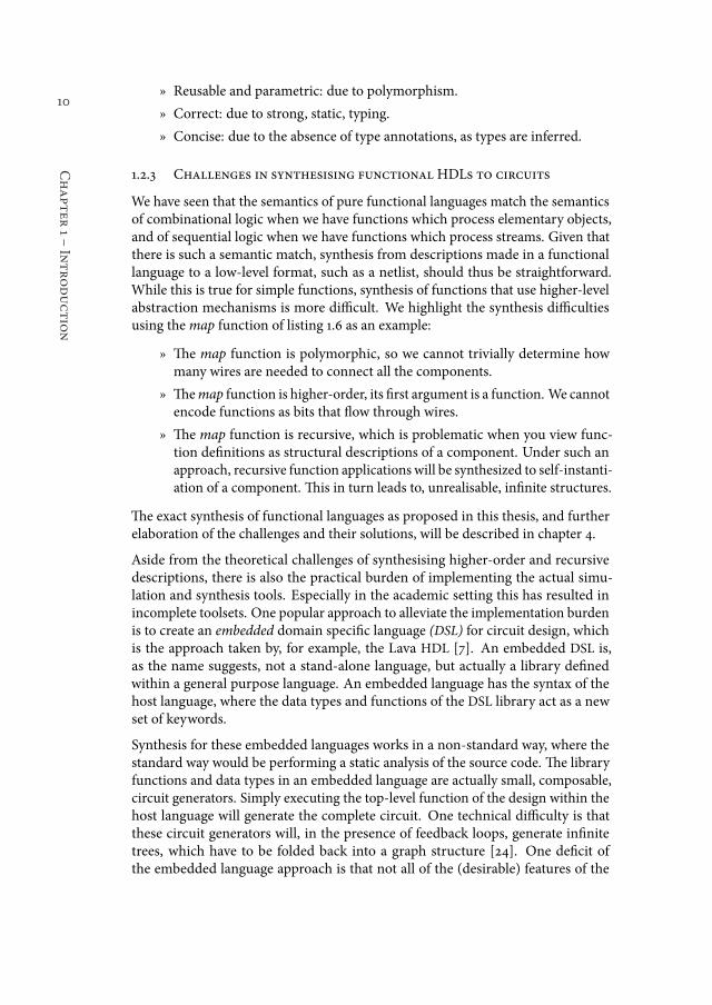
1 map f [] = []2 map f (x : xs) = f x : map f xs

Structural view

xNx�x�

f

x� x�

f f f f

Listing 1.6 ś map: parallel composition of a unary function

to hardware design need explicit descriptions of sequential logic. In chapter 2 wewill see approaches where functions are a purely behavioural description, and thesynthesis tool will infer, or generate, sequential logic where appropriate.

1.2.2 Higher level abstractions

While the semantic match between functional languages and digital circuits is agreat technical feature, it does not directly ofer the higher-level abstractions neededby hardware engineers to be productive. Where other high-level HDLs get theirnew design abstractions from the object-oriented programming paradigm, suchas classes and interfaces in SystemVerilog, functional HDLs gain their high level ofabstraction from their straightforward manipulation of functions. hese so-calledhigher-order functional languages have functions that can receive functions as theirarguments, or return functions as a result.

Higher-order functions allowmany forms of design abstraction. One example is, ofcourse, parametrising parts of the functionality of a circuit description. More gen-erally, it is possible to capture certain design and recursion patterns as a function;where the latter are called recursors. One such recursor is themap function, shownin listing 1.6, which takes two arguments, a function f and a list xs, and appliesthe f to all elements in xs. When we take a structural view of the map function(bottom part of listing 1.6), we see that application ofmap to a concrete function ftranslates to a parallel composition of the circuit f . Aside from parallel composi-tion, higher-order functions can capture many more connection and compositionpatterns commonly found in digital circuits. Further beneits of higher-order func-tions and recursors will be discussed in greater detail in chapter 3.

Another abstraction found in functional languages is polymorphism, where a func-tion is not tied to a ixed type for every argument, but can work on arguments ofany type. Combined with strong static typing and extensive and principled typeinference, designers can write functions that are:

10

Chapter

1śIntroduction

ż Reusable and parametric: due to polymorphism.

ż Correct: due to strong, static, typing.

ż Concise: due to the absence of type annotations, as types are inferred.

1.2.3 Challenges in synthesising functional HDLs to circuits

We have seen that the semantics of pure functional languages match the semanticsof combinational logic when we have functions which process elementary objects,and of sequential logic when we have functions which process streams. Given thatthere is such a semantic match, synthesis from descriptions made in a functionallanguage to a low-level format, such as a netlist, should thus be straightforward.While this is true for simple functions, synthesis of functions that use higher-levelabstraction mechanisms is more diicult. We highlight the synthesis diicultiesusing themap function of listing 1.6 as an example:

ż he map function is polymorphic, so we cannot trivially determine howmany wires are needed to connect all the components.

ż hemap function is higher-order, its irst argument is a function. We cannotencode functions as bits that low through wires.

ż he map function is recursive, which is problematic when you view func-tion deinitions as structural descriptions of a component. Under such anapproach, recursive function applications will be synthesized to self-instanti-ation of a component. his in turn leads to, unrealisable, ininite structures.

he exact synthesis of functional languages as proposed in this thesis, and furtherelaboration of the challenges and their solutions, will be described in chapter 4.

Aside from the theoretical challenges of synthesising higher-order and recursivedescriptions, there is also the practical burden of implementing the actual simu-lation and synthesis tools. Especially in the academic setting this has resulted inincomplete toolsets. One popular approach to alleviate the implementation burdenis to create an embedded domain speciic language (DSL) for circuit design, whichis the approach taken by, for example, the Lava HDL [7]. An embedded DSL is,as the name suggests, not a stand-alone language, but actually a library deinedwithin a general purpose language. An embedded language has the syntax of thehost language, where the data types and functions of the DSL library act as a newset of keywords.

Synthesis for these embedded languages works in a non-standard way, where thestandard way would be performing a static analysis of the source code. he libraryfunctions and data types in an embedded language are actually small, composable,circuit generators. Simply executing the top-level function of the design within thehost language will generate the complete circuit. One technical diiculty is thatthese circuit generators will, in the presence of feedback loops, generate ininitetrees, which have to be folded back into a graph structure [24]. One deicit ofthe embedded language approach is that not all of the (desirable) features of the

11

1.3śResea

rchquestions

host-language can be used for circuit description. Most importantly, the choice-constructs (such as case-statements) of the host language cannot be used to describechoice-constructs in the eventual circuit; we will elaborate why in chapter 2. Adesigner will have to use one of the choice-functions ofered by the embedded DSLlibrary; which are oten inferior in terms of expressibility compared to those oferedby the host language.

1.3 Research questions

hemain goal of this thesis is to further improve the productivity of circuit designers.As shown in the previous sections, there are multiple avenues we could explore inorder to achieve higher productivity. In this thesis we chose to further explore thedomain of functional hardware description languages, due to the semantic matchbetween functional languages and digital circuits, and the high-level abstractionmechanisms available in functional languages. Being more productive is, however,not just achieved by being able to abstract functionality, we also need:

ż To be able to express common idioms in circuit design straightforwardly.

ż Decrease the amount of time spent on the veriication of circuit designs.

ż Reason conidently about non-functional properties, such as chip area andgate propagation delays.

his thesis therefore seeks answers to the following questions:

ż How can functional languages be used to express both combinational andsequential circuits idiomatically?

ż How can we support correct-by-construction design methodologies usinga functional language?

ż How can we use the high-level abstractions without losing performance,and have a straightforward cost model?

1.4 Approach and contributions of the thesis

In a previous section we described the use of embedding in order to create a newHDL, but then also highlighted that the embedded approach has its own problems.Instead of either embedding a HDL in a functional language, or creating a com-pletely new language from scratch, this thesis explores the idea of using an existingfunctional language directly for the purpose of circuit description.

his thesis makes the choice of using the functional languageHaskell for circuit de-sign. We choose Haskell because of the many abstractions ofered by its expressivetype-system, polymorphism, higher-order functions, and pattern-matching con-structs. Haskell’s extensive type-derivation and near lack of syntax and keywordsadditionally leads to readable and concise circuit descriptions. Although there

12

Chapter

1śIntroduction

are other functional languages which have very similar properties, we speciicallychoose Haskell because:

ż It is a pure functional language, meaning that it has pure functions, which,as mentioned earlier, map very well to combinational logic.

ż It has a non-strict semantics, meaning that arguments to a function are onlyevaluated when their value is needed; the advantages of which are describedin chapter 3.

Also, instead of creating a complete toolset from scratch, we adapt an existingHaskell compiler. We start with the existing Glasgow Haskell compiler (GHC) [64]and its associated libraries and tools. We extend the set of libraries with a librarythat has circuit-speciic data types and functions, such as: arbitrary-width integers,registers, etc. Since our circuits are just Haskell programs, simulation is done inGHC by either:

ż Applying a circuit description to its inputs within the GHC Haskell inter-preter, or, if extra simulation speed is desired,

ż Compiling the circuit description, together with its inputs, into an (opti-mized) executable, and execute the compiled program.

Aside from having designed a library for circuit design, we have also created asynthesis tool that converts the Haskell descriptions to low-level, synthesisable,VHDL. Also for this synthesis tool we can reuse large parts of GHC, which exposesits internals as a library. Our eforts mainly focussed on the synthesis of GHCsintermediate language, which is much smaller than Haskell. We used the GHClibrary functions for parsing and type checking.

One advantage of embedded DSLs not explicitly discussed earlier is that the evalu-ation mechanism of the host-language eliminates all high-level abstractions, suchas higher-order functions. his means that the embedded DSL implementer doesnot have to deal with the synthesis of these abstractions. By choosing a standardsynthesis approach based on static analysis for this thesis, we do, however, have todeal with the synthesis of these abstraction mechanisms explicitly.

Contributions

For the synthesis of these higher-level abstraction mechanisms, we chose an ap-proach which is classic in the compilation of functional languages: compilation-by-transformation. In compilation-by-transformation, source-to-source transforma-tions are applied exhaustively until the description has such a shape that a mappingto the target architecture is straightforward. Existing approaches are designed withinstruction-set machines in mind: directly mapping their output to digital circuitswould lead to highly ineicient circuits. We will elaborate on these ineicienciesin chapter 4. his thesis explores a term rewrite system (TRS), a speciic form of

13

1.5śStru

ctureofthethesis

compilation-by-transformation, that removes abstraction mechanisms from a de-scription that have no direct mapping to a digital circuit, but without introducingany ineiciencies.

his thesis is a continuation of the work done in [4] and [38], which resulted inthe original prototype for the synthesis tool and circuit library: łCAES languagefor synchronous hardware (CλaSH)ž. We want to note that, from now on, we willrefer to the triple: Haskell, our library for circuit design, and our synthesis tool,as the CλaSH language. his thesis improves upon [4] and [38] by providing abetter approach for the composition of sequential circuit speciications, which wewill discuss in chapter 3. Additionally, the rewrite system described in chapter 4can correctly synthesise a larger class of speciications than the system describedin [38], and also comes with a correctness proof.

1.5 Structure of the thesis

he next chapter starts with an overview of a select number of hardware descrip-tion languages, focussing mostly on industrially used languages such as VHDL andVerilog, and on functional HDLs. he chapter will highlight the merits and disad-vantages of the individual languages, the details of their synthesis (and problemstherein), and compare them to the CλaSH language.

he subsequent chapter, chapter 3, describes the CλaSH language in greater detail.It highlights how the abstraction mechanisms in functional languages are highlybeneicial in the creation of high-level, parametric, circuit designs. One importantaspect discussed in length is how CλaSH deals with the concept of state. Addition-ally, we make our case for basing CλaSH on a non-strict language, as opposed to astrict language.

In chapter 4 we delve into the aspects of the synthesis from CλaSH to netlist-levelVHDL. We discuss both the general setup of the CλaSH compiler, and in greaterdepth the term rewrite system (TRS) that removes abstractions such as higher-order functionality. he chapter highlights the importance of types in synthesis,and how they guide the synthesis process. Correctness of the transformations,completeness of the system (that all abstractions with no counterpart in a digitalcircuit are removed), and termination of theCλaSH compiler, are important aspects,and are discussed in this chapter.

Usability and efectiveness of the CλaSH language and compiler are demonstratedin chapter 5 using several mid-size circuit designs. hese designs cover both dataand control oriented aspects found in digital circuits.

Finally, this thesis concludes with chapter 6, where we discuss and summarise whatwe have achieved by building theCλaSH language and compiler. Speciically, wewilladdress the advantages and disadvantages of using a general-purpose functionalprogramming language Haskell as a starting point for a HDL. he chapter endswith recommendations for further research.

14

15

2Hardware Description

Languages

Abstract ś In order to increase productivity, hardware description langua-ges must have the ability to abstract common idioms and patterns. Over theyears, conventional hardware description languages have acquired more meth-ods for abstraction, but these new aspects are sometimes non-trivial to use orare limited in scope as to what they are able to abstract. New languages havemore powerful abstraction mechanisms, but as a result, their synthesis to RTLhas become more complex, and is in certain situations limited. hese limita-tions in synthesis also limits the expressivity of the designer. We compare theabstraction capabilities of existing hardware description languages, and theirrespective limitations, and elaborate where CλaSH either makes improvementsor makes a diferent trade-of.

2.1 Introduction

here are many description languages for hardware, both analogue and digital, andtheir introduction and revision dates span several decades. In the context of thisthesis we will, however, focus on languages for synchronous, digital, circuit design;or at least those languages of which their synthesis tools produce a synchronousdigital circuit. We narrow the overview of HDLs and their comparison with theCλaSH language even further to those languages that are currently accepted inindustry (such as Verilog), and existing functional HDLs. he comparison withthe industrially accepted languages is there to warrant the research into new HDLsin general, where the comparison with functional HDLs is there to demonstrate

Parts of this chapter have been published in [CB:7] and [CB:13].

16

Chapter

2śHardwareDesc

ript

ionLanguages

that CλaSH captures a new and relevant point in the design space in the ield offunctional HDLs in particular.

For the languages such as VHDL and Verilog we describe the design abstractionavailable, and which parts of these languages are synthesisable. As CλaSH distin-guishes itself as a new point in the design space of functionalHDLs, we will describethese functional languages in more detail. Also their synthesis is discussed in moredetail, as this aspect usually plays an important role (and not an aterthought as itwas for VHDL) in the features available in these languages.

2.2 Standard hardware description languages

With standard languageswemeanHDLs that are commonly used in industry, taughtin courses on digital design, and have support in tools frommultiple vendors. heselanguages are: VHDL, Verilog, and by extension SystemVerilog.

2.2.1 VHDL

VHDL has several abstractions available that allow for parametric and generativecircuit design: generics (c.f. listing 2.1) and conigurations on the parametric side,and generate statements (c.f. listing 2.2) on the generative side. his section onlygives a short overview of these language features to demonstrate the means ofabstraction in VHDL. Completely elaborating these features falls outside the scopeof this thesis, and we refer the reader to works such as [3] for further details.

Parametrisation

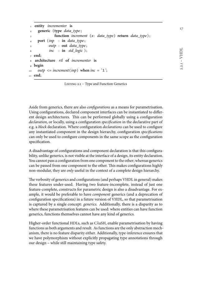
In VHDL, design entities can be parametrised by certain constant values usinggenerics. As ofVHDL-2008 [34], the generics have been extended to: type, function,and package generics. Type generics basically added a form of polymorphism tothe VHDL language, where function generics add higher-order functionality. Anexample of a polymorphic, higher-order, entity is shown in listing 2.1. here areseveral caveats to these new generics:

ż Support for VHDL-2008, especially for the new generics, is either non-existent or fairly limited in synthesis tools¹.

ż Functions only support the sequential subset of VHDL, not the concurrentone. here is hence no means to parametrise a component in concurrentlogic using generics, a designer must use conigurations for this.

ż Explicitly mapping every type generic is tedious and error-prone, especiallywhen compared to type-inference which is prevalent in functional langua-ges.

1At the time of this writing, the only synthesis tool that we have found to fully support type andfunction generics is: Synopsys Synplify(Pro/Premier), version I-2013.09-1

17

2.2.1śVHDL

1 entity incrementer is2 generic (type data_type ;3 function increment (x : data_type ) return data_type ) ;4 port ( inp : in data_type ;5 outp : out data_type ;6 inc : in std_logic ) ;7 end;8 architecture rtl of incrementer is9 begin

10 outp <= increment ( inp) when inc = ’1 ’;11 end;

Listing 2.1 ś Type and Function Generics

Aside from generics, there are also conigurations as a means for parametrisation.Using conigurations, declared component interfaces can be instantiated to difer-ent design architectures. his can be performed globally using a conigurationdeclaration, or locally, using a coniguration speciication in the declarative part ofe.g. a block declaration. Where coniguration declarations can be used to conigureany instantiated component in the design hierarchy, coniguration speciicationscan only be used to conigure components in the same scope as the conigurationspeciication.

A disadvantage of conigurations and component declaration is that this conigura-bility, unlike generics, is not visible at the interface of a design, its entity declaration.You cannot pass a coniguration fromone component to the other; whereas genericscan be passed from one component to the other. his makes conigurations highlynon-modular, they are only useful in the context of a complete design hierarchy.

he verbosity of generics and conigurations (and perhapsVHDL in general) makesthese features under-used. Having two feature-incomplete, instead of just onefeature-complete, constructs for parametric design is also a disadvantage. For ex-ample, it would be preferable to have component generics (and a deprecation ofconiguration speciications) in a future version of VHDL, so that parametrisationis captured by a single concept: generics. Additionally, there is a disparity as towhere these parametrisation features can be used: where entities can have functiongenerics, functions themselves cannot have any kind of generics.

Higher-order functional HDLs, such as CλaSH, enable parametrisation by havingfunctions as both arguments and result. As functions are the only abstractionmech-anism, there is no feature disparity either. Additionally, type-inference ensures thatwe have polymorphism without explicitly propagating type annotations throughour design ś while still maintaining type safety.

18

Chapter

2śHardwareDesc

ript

ionLanguages

Iterative generation: for ... generate

1 gen_label : for index in static_range generate

2 begin

3 ...4 end generate ;

Conditional generation: if ... generate

1 gen_label : if boolean_expression generate

2 begin

3 ...4 end generate ;

Listing 2.2 ś Iterative and Conditional generation in VHDL

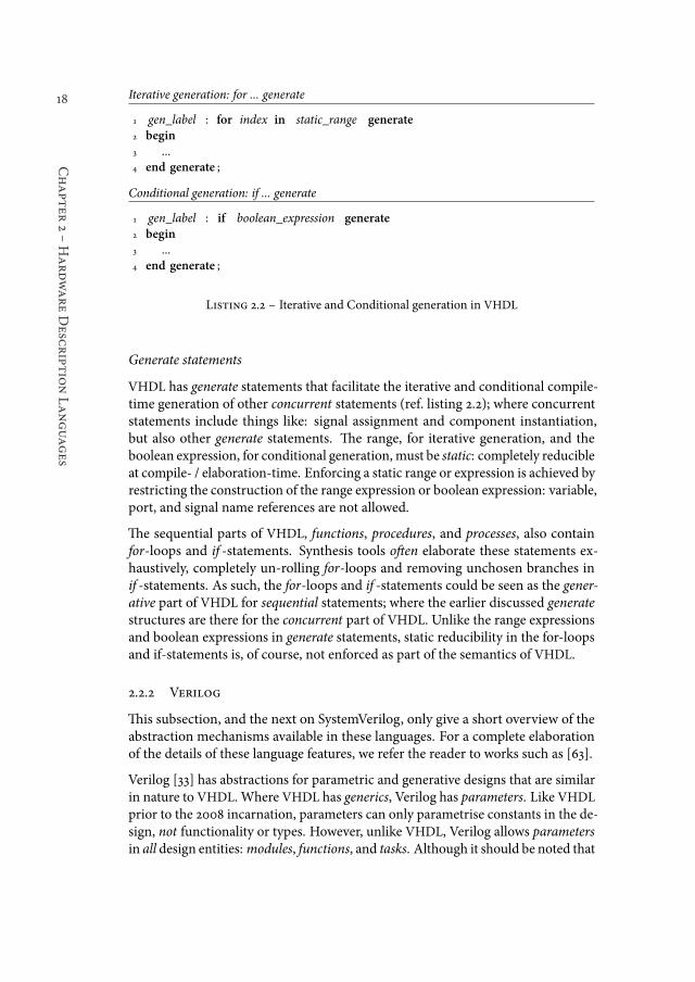
Generate statements

VHDL has generate statements that facilitate the iterative and conditional compile-time generation of other concurrent statements (ref. listing 2.2); where concurrentstatements include things like: signal assignment and component instantiation,but also other generate statements. he range, for iterative generation, and theboolean expression, for conditional generation, must be static: completely reducibleat compile- / elaboration-time. Enforcing a static range or expression is achieved byrestricting the construction of the range expression or boolean expression: variable,port, and signal name references are not allowed.

he sequential parts of VHDL, functions, procedures, and processes, also containfor-loops and if -statements. Synthesis tools oten elaborate these statements ex-haustively, completely un-rolling for-loops and removing unchosen branches inif -statements. As such, the for-loops and if -statements could be seen as the gener-ative part of VHDL for sequential statements; where the earlier discussed generatestructures are there for the concurrent part of VHDL. Unlike the range expressionsand boolean expressions in generate statements, static reducibility in the for-loopsand if-statements is, of course, not enforced as part of the semantics of VHDL.

2.2.2 Verilog

his subsection, and the next on SystemVerilog, only give a short overview of theabstraction mechanisms available in these languages. For a complete elaborationof the details of these language features, we refer the reader to works such as [63].

Verilog [33] has abstractions for parametric and generative designs that are similarin nature to VHDL. Where VHDL has generics, Verilog has parameters. Like VHDLprior to the 2008 incarnation, parameters can only parametrise constants in the de-sign, not functionality or types. However, unlike VHDL, Verilog allows parametersin all design entities: modules, functions, and tasks. Although it should be noted that

19

2.2.3śSystem

Verilog

tasks and functions in Verilog can only exist within amodule, and are not top-leveldesign entities; functions in VHDL are top-level design entities. Verilog also hasconigurations; however, where VHDL allows coniguration speciications within anarchitecture, Verilog only supports conigurations as a top-level construct.

Generative constructs, in the form of generate blocks, support both conditionaland iterative generation. Aside from boolean conditions, Verilog also supportscase-statements as conditional generation blocks.

Being related to the C programming language, Verilog also has compile-timema-cros through a pre-processor. Using ‘define and ‘ifdef...‘else...‘endif,code can be conditionally synthesised; and could hence be classiied as a (condi-tional) generative construct of Verilog. An advantage ofmacros over generate blocksis thatmacros can be used outside of a module deinition, e.g. to conditionally gen-erate a module interface. An advantage of generate blocks is that they enable twodiferent instances of the same module to be conigured individually.

2.2.3 SystemVerilog

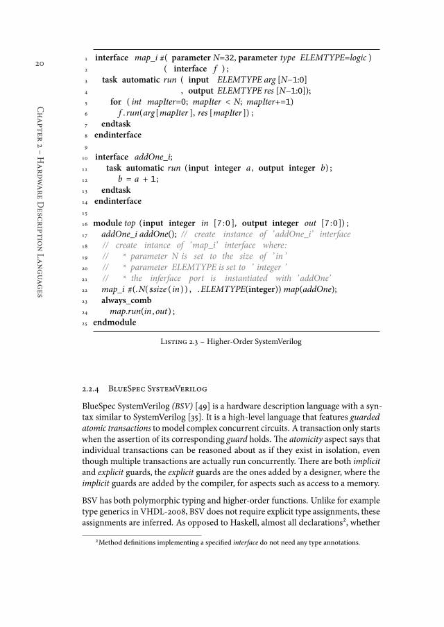
SystemVerilog is a proper extension to Verilog, and since 2009 the two languagesare merged into the IEEE standard 1800-2009; there is now only SystemVerilog.SystemVerilog extends Verilog parameters with type parameters, hence supportingpolymorphic designs. Support for these type parameters is present in both FPGAand ASIC tooling. Unlike VHDL-2008, there are no function or task parameters.his does not mean that functionality cannot be abstracted: SystemVerilog intro-duces a new design element called an interface.

An interface can bundle, aside from ports and wires, functionality in the form offunctions, tasks, and procedural blocks. Unlikemodules, interfaces can be made intoports; for both modules and interfaces themselves. hese interface ports can alsobe generic, meaning that the choice for a concrete interface is deferred to when amodule (or higher-level interface) is instantiated. Listing 2.3 showcases all of theabove points. he interface map_i has a generic interface port, f. Nota bene, theinterface f should have a task or function called run, which is called on line 6. hemap_i interface is hence parametrised over the run task, or function, ofered bythe interface f. Finally, on line 17, a concrete instance of the addOne_i interface iscreated, which is subsequently passed to a concrete instance of themap_i interfaceon line 22.

Although the presented SystemVerilog code is certainly not idiomatic, ASIC synthe-sis tools are able to generate a netlist for Listing 2.3. he presented technique doesnot facilitate the abstraction over all the types of behaviour in SystemVerilog. Tasksand functions only allow a subset of SystemVerilog within their bodies: for example,tasks cannot have procedural blocks such as always_comb. Further investigation isthe higher-order possibilities of SystemVerilog are hence warranted.

20

Chapter

2śHardwareDesc

ript

ionLanguages

1 interface map_i #( parameter N=32, parameter type ELEMTYPE=logic )2 ( interface f ) ;3 task automatic run ( input ELEMTYPE arg [N−1:0]4 , output ELEMTYPE res [N−1:0]);5 for ( int mapIter=0; mapIter < N; mapIter+=1)6 f . run(arg[mapIter ], res [mapIter ]) ;7 endtask8 endinterface9

10 interface addOne_i;11 task automatic run (input integer a , output integer b) ;12 b = a + 1 ;13 endtask14 endinterface15

16 module top (input integer in [7 :0 ], output integer out [7 :0]) ;17 addOne_i addOne(); // create instance of ’ addOne_i’ interface18 // create intance of ’map_i’ interface where:19 // * parameter N is set to the size of ’ in ’20 // * parameter ELEMTYPE is set to ’ integer ’21 // * the inferface port is instantiated with ’addOne’22 map_i #(.N($size ( in ) ) , .ELEMTYPE(integer))map(addOne);23 always_comb24 map.run(in ,out) ;25 endmodule

Listing 2.3 ś Higher-Order SystemVerilog

2.2.4 BlueSpec SystemVerilog

BlueSpec SystemVerilog (BSV) [49] is a hardware description language with a syn-tax similar to SystemVerilog [35]. It is a high-level language that features guardedatomic transactions tomodel complex concurrent circuits. A transaction only startswhen the assertion of its corresponding guard holds. he atomicity aspect says thatindividual transactions can be reasoned about as if they exist in isolation, eventhough multiple transactions are actually run concurrently. here are both implicitand explicit guards, the explicit guards are the ones added by a designer, where theimplicit guards are added by the compiler, for aspects such as access to a memory.

BSV has both polymorphic typing and higher-order functions. Unlike for exampletype generics inVHDL-2008, BSV does not require explicit type assignments, theseassignments are inferred. As opposed to Haskell, almost all declarations², whether

2Method deinitions implementing a speciied interface do not need any type annotations.

21

2.3śFu

nctionalLanguages

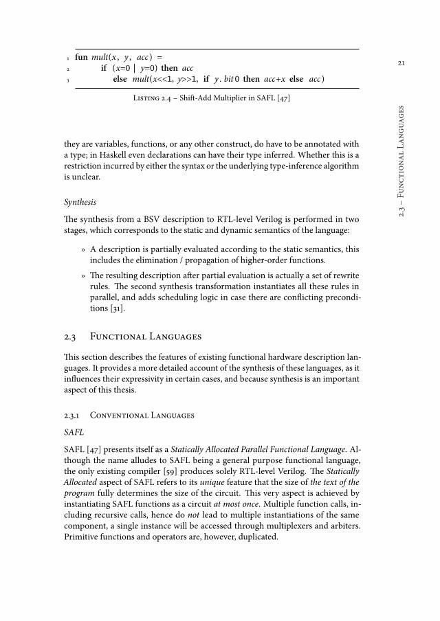
1 fun mult(x , y , acc ) =2 if (x=0 | y=0) then acc3 else mult(x<<1, y>>1, if y . bit 0 then acc+x else acc )

Listing 2.4 ś Shit-Add Multiplier in SAFL [47]

they are variables, functions, or any other construct, do have to be annotated witha type; in Haskell even declarations can have their type inferred. Whether this is arestriction incurred by either the syntax or the underlying type-inference algorithmis unclear.

Synthesis

he synthesis from a BSV description to RTL-level Verilog is performed in twostages, which corresponds to the static and dynamic semantics of the language:

ż A description is partially evaluated according to the static semantics, thisincludes the elimination / propagation of higher-order functions.

ż he resulting description ater partial evaluation is actually a set of rewriterules. he second synthesis transformation instantiates all these rules inparallel, and adds scheduling logic in case there are conlicting precondi-tions [31].

2.3 Functional Languages

his section describes the features of existing functional hardware description lan-guages. It provides a more detailed account of the synthesis of these languages, as itinluences their expressivity in certain cases, and because synthesis is an importantaspect of this thesis.

2.3.1 Conventional Languages

SAFL

SAFL [47] presents itself as a Statically Allocated Parallel Functional Language. Al-though the name alludes to SAFL being a general purpose functional language,the only existing compiler [59] produces solely RTL-level Verilog. he StaticallyAllocated aspect of SAFL refers to its unique feature that the size of the text of theprogram fully determines the size of the circuit. his very aspect is achieved byinstantiating SAFL functions as a circuit at most once. Multiple function calls, in-cluding recursive calls, hence do not lead to multiple instantiations of the samecomponent, a single instance will be accessed through multiplexers and arbiters.Primitive functions and operators are, however, duplicated.

22

Chapter

2śHardwareDesc

ript

ionLanguages

Calls to f are serialised

1 fun f x = ...2 fun main(x,y) = g( f (x) , f (y) )

Duplication of f leads to parallel execution

1 fun f x = ...2 fun f ’ x = ...3 fun main(x,y) = g( f (x) , f ’( y) )

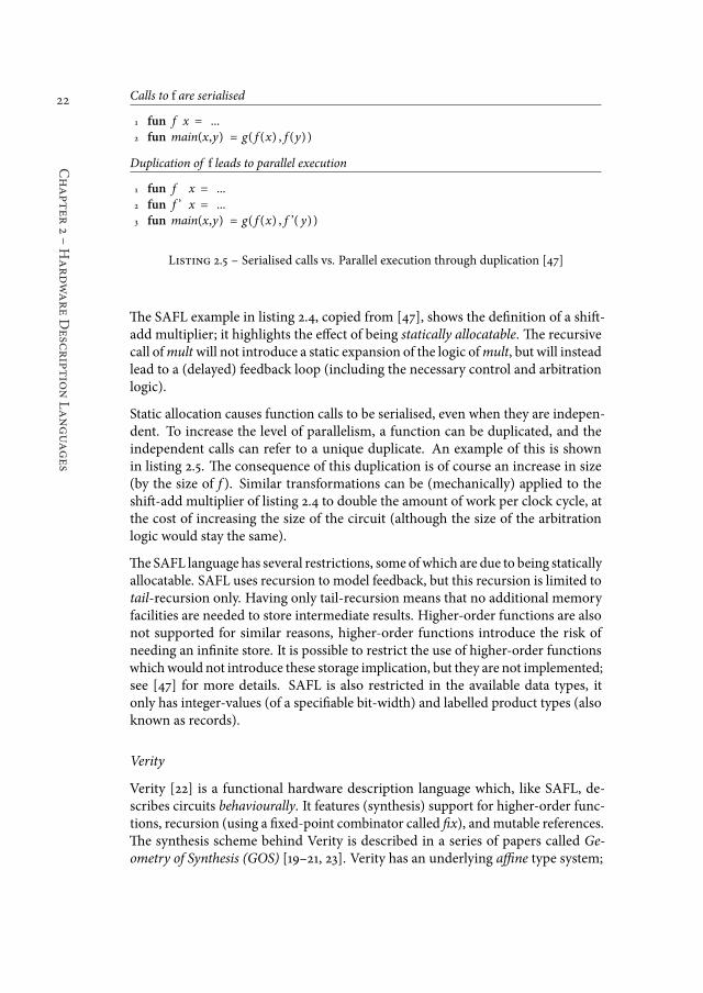
Listing 2.5 ś Serialised calls vs. Parallel execution through duplication [47]

he SAFL example in listing 2.4, copied from [47], shows the deinition of a shit-add multiplier; it highlights the efect of being statically allocatable. he recursivecall ofmult will not introduce a static expansion of the logic ofmult, but will insteadlead to a (delayed) feedback loop (including the necessary control and arbitrationlogic).

Static allocation causes function calls to be serialised, even when they are indepen-dent. To increase the level of parallelism, a function can be duplicated, and theindependent calls can refer to a unique duplicate. An example of this is shownin listing 2.5. he consequence of this duplication is of course an increase in size(by the size of f ). Similar transformations can be (mechanically) applied to theshit-add multiplier of listing 2.4 to double the amount of work per clock cycle, atthe cost of increasing the size of the circuit (although the size of the arbitrationlogic would stay the same).

he SAFL language has several restrictions, some ofwhich are due to being staticallyallocatable. SAFL uses recursion to model feedback, but this recursion is limited totail-recursion only. Having only tail-recursion means that no additional memoryfacilities are needed to store intermediate results. Higher-order functions are alsonot supported for similar reasons, higher-order functions introduce the risk ofneeding an ininite store. It is possible to restrict the use of higher-order functionswhichwould not introduce these storage implication, but they are not implemented;see [47] for more details. SAFL is also restricted in the available data types, itonly has integer-values (of a speciiable bit-width) and labelled product types (alsoknown as records).

Verity

Verity [22] is a functional hardware description language which, like SAFL, de-scribes circuits behaviourally. It features (synthesis) support for higher-order func-tions, recursion (using a ixed-point combinator called ix), andmutable references.he synthesis scheme behind Verity is described in a series of papers called Ge-ometry of Synthesis (GOS) [19ś21, 23]. Verity has an underlying aine type system;

23

2.3.1śConventionalLanguages

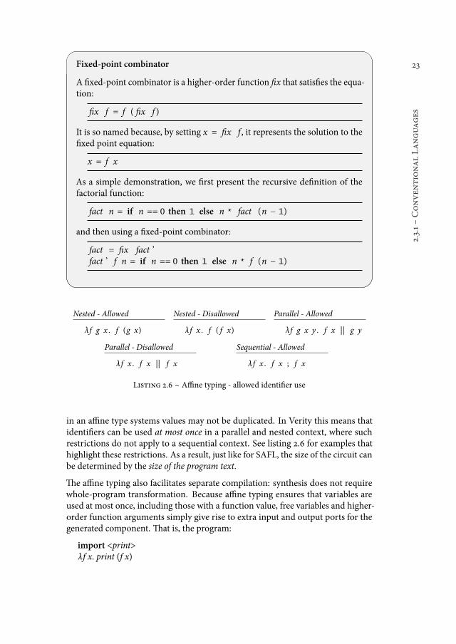
Fixed-point combinator

A ixed-point combinator is a higher-order function ix that satisies the equa-tion:

ix f = f ( ix f )

It is so named because, by setting x = ix f , it represents the solution to theixed point equation:

x = f x

As a simple demonstration, we irst present the recursive deinition of thefactorial function:

fact n = if n == 0 then 1 else n * fact (n − 1)

and then using a ixed-point combinator:

fact = ix fact ’fact ’ f n = if n == 0 then 1 else n * f (n − 1)

Nested - Allowed

λf g x . f (g x)

Nested - Disallowed

λf x . f ( f x)

Parallel - Allowed

λf g x y . f x || g y

Parallel - Disallowed

λf x . f x || f x

Sequential - Allowed

λf x . f x ; f x

Listing 2.6 ś Aine typing - allowed identiier use

in an aine type systems values may not be duplicated. In Verity this means thatidentiiers can be used at most once in a parallel and nested context, where suchrestrictions do not apply to a sequential context. See listing 2.6 for examples thathighlight these restrictions. As a result, just like for SAFL, the size of the circuit canbe determined by the size of the program text.

he aine typing also facilitates separate compilation: synthesis does not requirewhole-program transformation. Because aine typing ensures that variables areused at most once, including those with a function value, free variables and higher-order function arguments simply give rise to extra input and output ports for thegenerated component. hat is, the program:

import <print>λf x. print (f x)

24

Chapter

2śHardwareDesc

ript

ionLanguages

lib1.ia

import <print>let f = λx. print xin export f

lib2.ia

import <print>let g = λx. print xin export g

main.ia

import "lib1"import "lib2"

#Will error with:# lib1.ia: ‘print‘ already used in ‘lib2.ia‘f 4; g 7

Listing 2.7 ś Invalid linking

Gives rise to a component with the obvious input port for x, and an output port forthe result (in this case just a control signal, a ready lag), but also:

ż An output port corresponding to the input of f, and an input port corre-sponding to the output of f.

ż An output port corresponding to the input of print, and an input port cor-responding to the output of print.

During link time all the components are properly connected. he linking processdoes, however, not resolve any potential conlicts, such as the conlict shown inlisting 2.7. In this case the functions f and g both use the print function, and thelinker cannot connect the single print component to the f and g components; eventhoughmain uses f and g in a sequential fashion.

Although the aine typing rules seem overly cumbersome, especially the nested ap-plication restriction (λf x. f (f x)), the developer-facing type system is actually morelenient. he Verity compiler uses a process called serialisation [21] that transforms,

ż he non-aine expression:

let f = λg x . g (g x) in f (λy. y + 1) 0

ż To the aine expression:

let f = λg h x . g (h x) in f (λy. y + 1) (λy. y + 1) 0

At themoment, recursion inVerity is only possible using theixed-point combinator,ix. Recursion using ix is always unfolded in time. So, the circuit derived from thedescription given in listing 2.8, contains all the logic needed for one instantiation ofthe body of ix. Just like in SAFL, control logic is added so that the circuit exhibitsthe behaviour of the recursive description.

25

2.3.1śConventionalLanguages

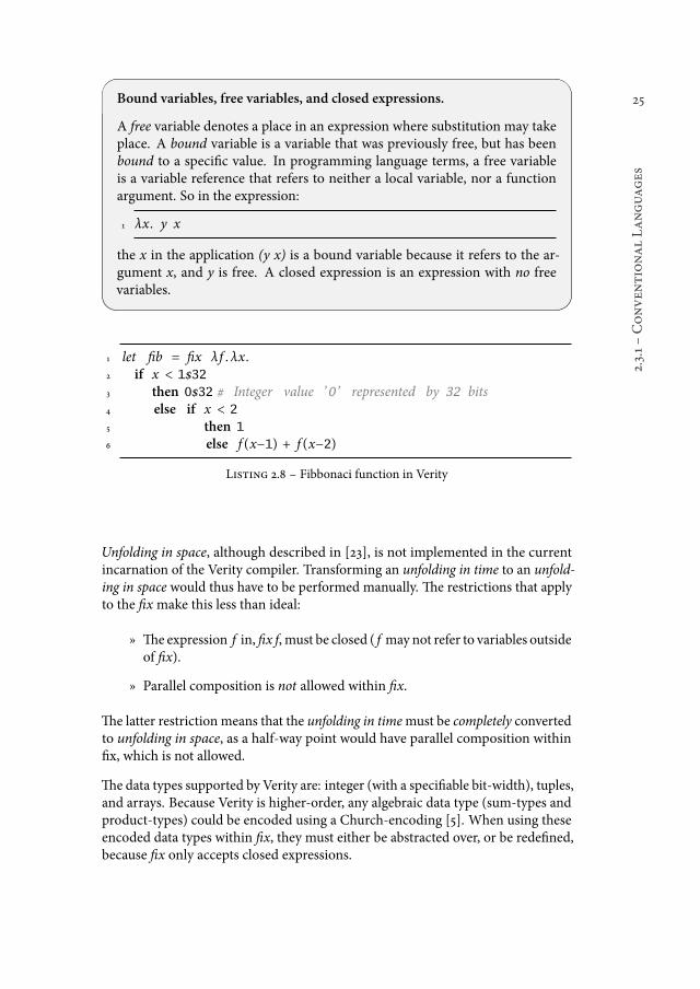
Bound variables, free variables, and closed expressions.

A free variable denotes a place in an expression where substitution may takeplace. A bound variable is a variable that was previously free, but has beenbound to a speciic value. In programming language terms, a free variableis a variable reference that refers to neither a local variable, nor a functionargument. So in the expression:

1 λx. y x

the x in the application (y x) is a bound variable because it refers to the ar-gument x, and y is free. A closed expression is an expression with no freevariables.

1 let ib = ix λf . λx.2 if x < 1$323 then 0$32 # Integer value ’0 ’ represented by 32 bits4 else if x < 2

5 then 1

6 else f (x−1) + f (x−2)

Listing 2.8 ś Fibbonaci function in Verity

Unfolding in space, although described in [23], is not implemented in the currentincarnation of the Verity compiler. Transforming an unfolding in time to an unfold-ing in space would thus have to be performed manually. he restrictions that applyto the ixmake this less than ideal:

ż he expression f in, ix f, must be closed ( f maynot refer to variables outsideof ix).

ż Parallel composition is not allowed within ix.

he latter restriction means that the unfolding in timemust be completely convertedto unfolding in space, as a half-way point would have parallel composition withinix, which is not allowed.

he data types supported by Verity are: integer (with a speciiable bit-width), tuples,and arrays. Because Verity is higher-order, any algebraic data type (sum-types andproduct-types) could be encoded using a Church-encoding [5]. When using theseencoded data types within ix, they must either be abstracted over, or be redeined,because ix only accepts closed expressions.

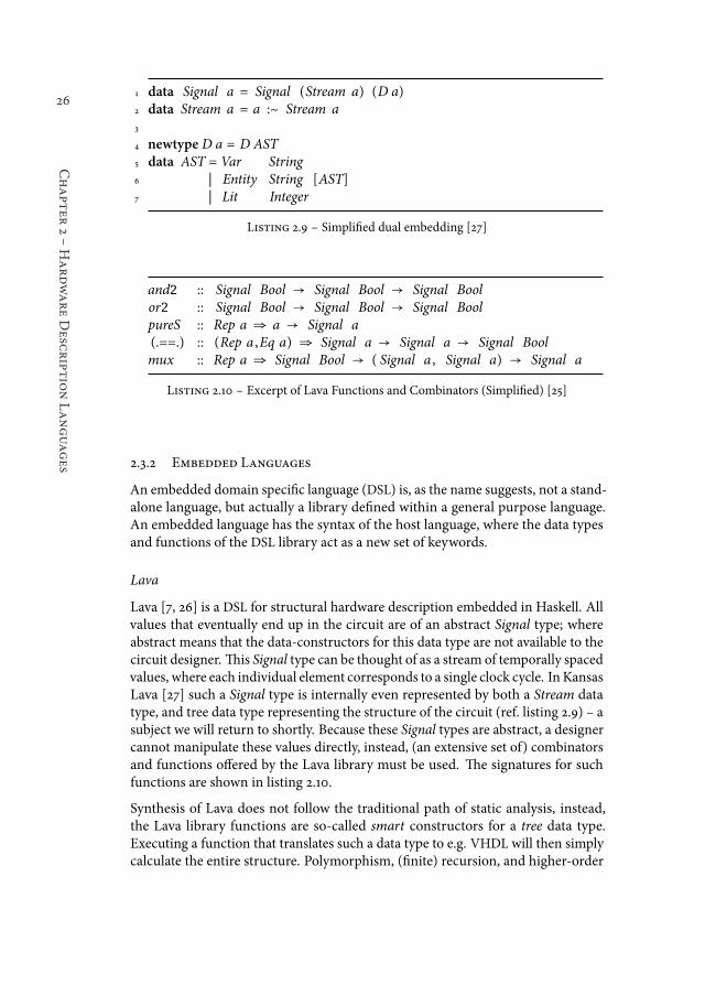
26

Chapter

2śHardwareDesc

ript

ionLanguages

1 data Signal a = Signal (Stream a) (D a)2 data Stream a = a :~ Stream a3

4 newtype D a = D AST5 data AST = Var String6 | Entity String [AST]7 | Lit Integer

Listing 2.9 ś Simpliied dual embedding [27]

and2 :: Signal Bool → Signal Bool → Signal Boolor2 :: Signal Bool → Signal Bool → Signal BoolpureS :: Rep a ⇒ a → Signal a(.==.) :: (Rep a ,Eq a) ⇒ Signal a → Signal a → Signal Boolmux :: Rep a ⇒ Signal Bool → ( Signal a , Signal a) → Signal a

Listing 2.10 ś Excerpt of Lava Functions and Combinators (Simpliied) [25]

2.3.2 Embedded Languages

An embedded domain speciic language (DSL) is, as the name suggests, not a stand-alone language, but actually a library deined within a general purpose language.An embedded language has the syntax of the host language, where the data typesand functions of the DSL library act as a new set of keywords.

Lava

Lava [7, 26] is a DSL for structural hardware description embedded in Haskell. Allvalues that eventually end up in the circuit are of an abstract Signal type; whereabstract means that the data-constructors for this data type are not available to thecircuit designer. his Signal type can be thought of as a stream of temporally spacedvalues, where each individual element corresponds to a single clock cycle. InKansasLava [27] such a Signal type is internally even represented by both a Stream datatype, and tree data type representing the structure of the circuit (ref. listing 2.9) ś asubject we will return to shortly. Because these Signal types are abstract, a designercannot manipulate these values directly, instead, (an extensive set of) combinatorsand functions ofered by the Lava library must be used. he signatures for suchfunctions are shown in listing 2.10.

Synthesis of Lava does not follow the traditional path of static analysis, instead,the Lava library functions are so-called smart constructors for a tree data type.Executing a function that translates such a data type to e.g. VHDL will then simplycalculate the entire structure. Polymorphism, (inite) recursion, and higher-order

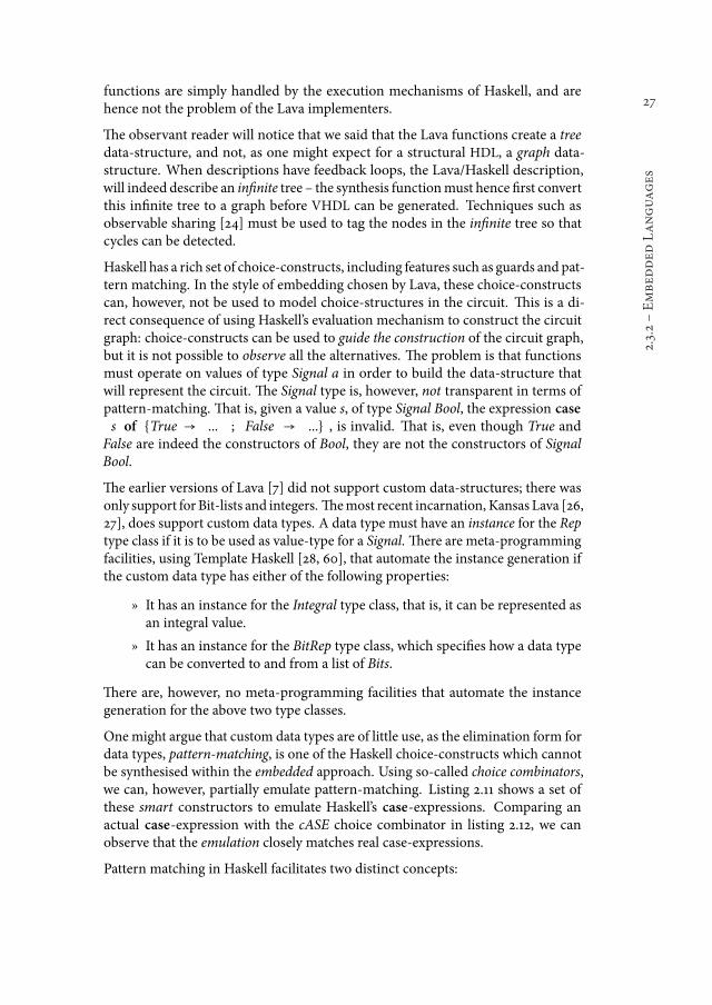
27

2.3.2śEmbed

ded

Languages

functions are simply handled by the execution mechanisms of Haskell, and arehence not the problem of the Lava implementers.

he observant reader will notice that we said that the Lava functions create a treedata-structure, and not, as one might expect for a structural HDL, a graph data-structure. When descriptions have feedback loops, the Lava/Haskell description,will indeed describe an ininite tree ś the synthesis functionmust hence irst convertthis ininite tree to a graph before VHDL can be generated. Techniques such asobservable sharing [24] must be used to tag the nodes in the ininite tree so thatcycles can be detected.

Haskell has a rich set of choice-constructs, including features such as guards and pat-tern matching. In the style of embedding chosen by Lava, these choice-constructscan, however, not be used to model choice-structures in the circuit. his is a di-rect consequence of using Haskell’s evaluation mechanism to construct the circuitgraph: choice-constructs can be used to guide the construction of the circuit graph,but it is not possible to observe all the alternatives. he problem is that functionsmust operate on values of type Signal a in order to build the data-structure thatwill represent the circuit. he Signal type is, however, not transparent in terms ofpattern-matching. hat is, given a value s, of type Signal Bool, the expression cases of {True → ... ; False → ...} , is invalid. hat is, even though True andFalse are indeed the constructors of Bool, they are not the constructors of SignalBool.

he earlier versions of Lava [7] did not support custom data-structures; there wasonly support for Bit-lists and integers. hemost recent incarnation, Kansas Lava [26,27], does support custom data types. A data type must have an instance for the Reptype class if it is to be used as value-type for a Signal. here are meta-programmingfacilities, using Template Haskell [28, 60], that automate the instance generation ifthe custom data type has either of the following properties:

ż It has an instance for the Integral type class, that is, it can be represented asan integral value.

ż It has an instance for the BitRep type class, which speciies how a data typecan be converted to and from a list of Bits.

here are, however, no meta-programming facilities that automate the instancegeneration for the above two type classes.

One might argue that custom data types are of little use, as the elimination form fordata types, pattern-matching, is one of the Haskell choice-constructs which cannotbe synthesised within the embedded approach. Using so-called choice combinators,we can, however, partially emulate pattern-matching. Listing 2.11 shows a set ofthese smart constructors to emulate Haskell’s case-expressions. Comparing anactual case-expression with the cASE choice combinator in listing 2.12, we canobserve that the emulation closely matches real case-expressions.

Pattern matching in Haskell facilitates two distinct concepts:

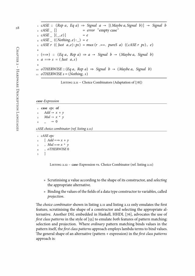
28

Chapter

2śHardwareDesc

ript

ionLanguages

1 cASE :: (Rep a , Eq a) ⇒ Signal a → [(Maybe a, Signal b)] → Signal b2 cASE _ [] = error "empty case "3 cASE _ [(_ ,e) ] = e4 cASE _ ((Nothing , e) :_) = e5 cASE r (( Just a ,e) : ps) = mux (r .==. pureS a) ((cASE r ps) , e)6

7 (=⇒) :: (Eq a , Rep a) ⇒ a → Signal b → (Maybe a, Signal b)8 a =⇒ s = ( Just a , s )9

10 oTHERWISE :: (Eq a, Rep a) ⇒ Signal b → (Maybe a, Signal b)11 oTHERWISE s = (Nothing, s )

Listing 2.11 ś Choice Combinators (Adaptation of [78])

case-Expression

1 case opc of

2 Add→ x + y3 Mul→ x * y4 _ → 0

cASE choice combinator (ref. listing 2.11)

1 cASE opc2 [ Add =⇒ x + y3 , Mul =⇒ x * y4 , oTHERWISE 0

5 ]

Listing 2.12 ś case-Expression vs. Choice Combinator (ref. listing 2.11)

ż Scrutinising a value according to the shape of its constructor, and selectingthe appropriate alternative.

ż Binding the values of the ields of a data type constructor to variables, calledprojection.

he choice combinator shown in listing 2.11 and listing 2.12 only emulates the irstfeature, scrutinising the shape of a constructor and selecting the appropriate al-ternative. Another DSL embedded in Haskell, HHDL [76], advocates the use ofirst class patterns in the style of [55] to emulate both features of pattern matching:selection and projection. Where ordinary pattern matching binds values in thepattern itself, the irst class patterns approach employs lambda terms to bind values.he general shape of an alternative (pattern + expression) in the irst class patternsapproach is:

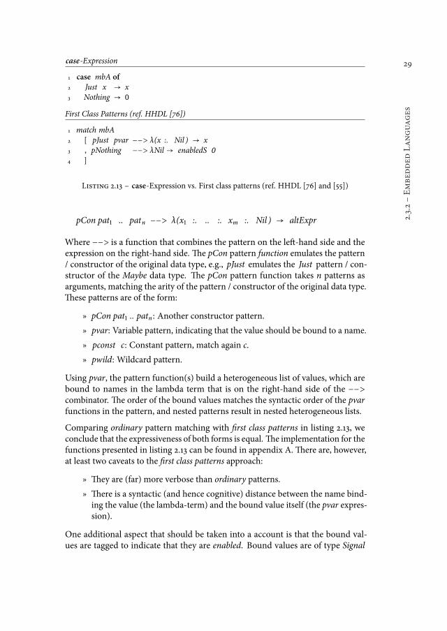
29

2.3.2śEmbed

ded

Languages

case-Expression

1 case mbA of

2 Just x → x3 Nothing → 0

First Class Patterns (ref. HHDL [76])

1 match mbA2 [ pJust pvar −−> λ(x :. Nil ) → x3 , pNothing −−> λNil → enabledS 0

4 ]

Listing 2.13 ś case-Expression vs. First class patterns (ref. HHDL [76] and [55])

pCon pat1 .. patn −−> λ(x1 :. .. :. xm :. Nil ) → altExpr

Where −−> is a function that combines the pattern on the let-hand side and theexpression on the right-hand side. he pCon pattern function emulates the pattern/ constructor of the original data type, e.g., pJust emulates the Just pattern / con-structor of the Maybe data type. he pCon pattern function takes n patterns asarguments, matching the arity of the pattern / constructor of the original data type.hese patterns are of the form:

ż pCon pat1 .. patn : Another constructor pattern.

ż pvar: Variable pattern, indicating that the value should be bound to a name.

ż pconst c: Constant pattern, match again c.

ż pwild: Wildcard pattern.

Using pvar, the pattern function(s) build a heterogeneous list of values, which arebound to names in the lambda term that is on the right-hand side of the −−>combinator. he order of the bound values matches the syntactic order of the pvarfunctions in the pattern, and nested patterns result in nested heterogeneous lists.

Comparing ordinary pattern matching with irst class patterns in listing 2.13, weconclude that the expressiveness of both forms is equal. he implementation for thefunctions presented in listing 2.13 can be found in appendix A. here are, however,at least two caveats to the irst class patterns approach:

ż hey are (far) more verbose than ordinary patterns.

ż here is a syntactic (and hence cognitive) distance between the name bind-ing the value (the lambda-term) and the bound value itself (the pvar expres-sion).

One additional aspect that should be taken into a account is that the bound val-ues are tagged to indicate that they are enabled. Bound values are of type Signal

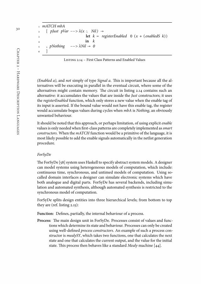
30

Chapter

2śHardwareDesc

ript

ionLanguages

1 mATCH mbA2 [ pJust pVar −−> λ(x :. Nil ) →3 let k = registerEnabled 0 (x + (enabledS k))4 in k5 , pNothing −−> λNil → 0

6 ]

Listing 2.14 ś First Class Patterns and Enabled Values

(Enabled a), and not simply of type Signal a. his is important because all the al-ternatives will be executing in parallel in the eventual circuit, where some of thealternatives might contain memory. he circuit in listing 2.14 contains such analternative: it accumulates the values that are inside the Just constructors; it usesthe registerEnabled function, which only stores a new value when the enable tag ofits input is asserted. If the bound value would not have this enable tag, the registerwould accumulate bogus values during cycles whenmbA is Nothing, an obviouslyunwanted behaviour.

It should be noted that this approach, or perhaps limitation, of using explicit enablevalues is only neededwhen irst-class patterns are completely implemented as smartconstructors. When themATCH function would be a primitive of the language, it ismost likely possible to add the enable signals automatically in the netlist generationprocedure.

ForSyDe

heForSyDe [58] system usesHaskell to specify abstract systemmodels. A designercan model systems using heterogeneous models of computation, which include:continuous time, synchronous, and untimed models of computation. Using so-called domain interfaces a designer can simulate electronic systems which haveboth analogue and digital parts. ForSyDe has several backends, including simu-lation and automated synthesis, although automated synthesis is restricted to thesynchronous model of computation.

ForSyDe splits design entities into three hierarchical levels; from bottom to topthey are (ref. listing 2.15):

Function: Deines, partially, the internal behaviour of a process.

Process: he main design unit in ForSyDe. Processes consist of values and func-tions which determine its state and behaviour. Processes can only be createdusing well-deined process constructors. An example of such a process con-structor ismealySY, which takes two functions, one that calculates the nextstate and one that calculates the current output, and the value for the initialstate. his process then behaves like a standardMealymachine [44].

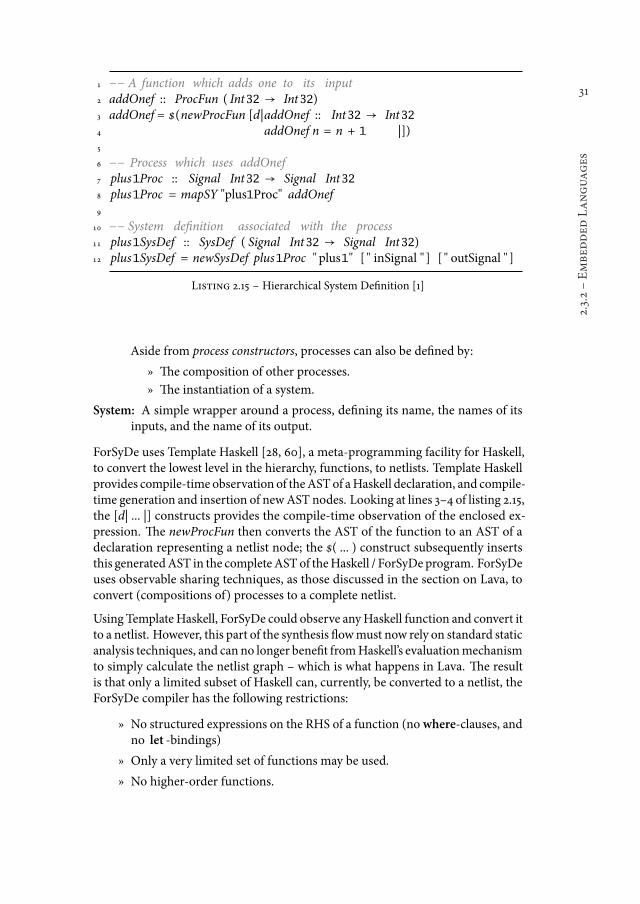
31

2.3.2śEmbed

ded

Languages

1 −− A function which adds one to its input2 addOnef :: ProcFun ( Int32 → Int32)3 addOnef = $(newProcFun [d|addOnef :: Int32 → Int324 addOnef n = n + 1 |])5

6 −− Process which uses addOnef7 plus1Proc :: Signal Int32 → Signal Int328 plus1Proc = mapSY "plus1Proc" addOnef9

10 −− System deinition associated with the process11 plus1SysDef :: SysDef ( Signal Int32 → Signal Int32)12 plus1SysDef = newSysDef plus1Proc " plus1" [ " inSignal " ] [ " outSignal " ]

Listing 2.15 ś Hierarchical System Deinition [1]

Aside from process constructors, processes can also be deined by:

ż he composition of other processes.

ż he instantiation of a system.

System: A simple wrapper around a process, deining its name, the names of itsinputs, and the name of its output.

ForSyDe uses Template Haskell [28, 60], a meta-programming facility for Haskell,to convert the lowest level in the hierarchy, functions, to netlists. Template Haskellprovides compile-time observation of theASTof aHaskell declaration, and compile-time generation and insertion of newAST nodes. Looking at lines 3ś4 of listing 2.15,the [d| ... |] constructs provides the compile-time observation of the enclosed ex-pression. he newProcFun then converts the AST of the function to an AST of adeclaration representing a netlist node; the $( ... ) construct subsequently insertsthis generatedAST in the completeASTof theHaskell / ForSyDe program. ForSyDeuses observable sharing techniques, as those discussed in the section on Lava, toconvert (compositions of) processes to a complete netlist.

Using TemplateHaskell, ForSyDe could observe anyHaskell function and convert itto a netlist. However, this part of the synthesis lowmust now rely on standard staticanalysis techniques, and can no longer beneit fromHaskell’s evaluationmechanismto simply calculate the netlist graph ś which is what happens in Lava. he resultis that only a limited subset of Haskell can, currently, be converted to a netlist, theForSyDe compiler has the following restrictions:

ż No structured expressions on the RHS of a function (nowhere-clauses, andno let -bindings)

ż Only a very limited set of functions may be used.

ż No higher-order functions.

32

Chapter

2śHardwareDesc

ript

ionLanguages

ż No pattern-matching in a function deinition

ż Patterns in case-statements are limited to literals, variables, and wildcards;constructor-patterns are not supported.

ż No type-class methods.

ż No support for guards.

ForSyDe does support synthesis of custom data types, but without pattern-match-ing on constructors, their usefulness is reduced.

2.4 Conclusions

2.4.1 Standard Languages

he standard hardware description languages all allow type and function parame-trisation in some shape or form. A recurring theme in all of these languages is thatthe type parameters have to be speciically annotated. In Haskell, and by extensionCλaSH, types are automatically inferred. his type inference relieves the designerfrom the cognitive burden of:

ż Determining the types of all values, whether they be for input or outputports, or wires.

ż Determining which types must be parametrised to get the most generalhardware design.

here is an additional syntactic burden in the standard languages of having toexplicitly instantiate all the parameters. In CλaSH, this instantiation happens auto-matically, thereby improving the readability of hardware designs.

Also, although functionality can be parametrised in the standard languages, func-tions are not irst-class. As a result, parametrising functionality is not really encour-aged by the language:

ż here is no single, straightforward, parametrisation mechanism. In VHDL,depending on the type of logic you want to parametrise, you should eitheruse conigurations, or function generics. heir distinct disadvantages havebeen described in an earlier section.

ż In SystemVerilog, modules and interfaces can only be parametrised in termsof interfaces, not modules. Even though modules are considered the defaultdesign entities, exempliied by the fact that the top-level design entity mustbe a module.

In CλaSH, where functions are irst-class, and also the only design entities, theserestrictions do not apply. Designers also do not have to learn and use a new syn-tax to parametrise functionality: function arguments, on both the abstraction andapplication side, are indistinguishable from other arguments. his irst-class ap-proach lowers the barrier to parametrise functionality, and thereby encourages thecreation of generic, reusable, hardware descriptions.

33

2.4.2śFu

nctionalLanguages

2.4.2 Functional Languages

Conventional

SAFL is a irst-order functional language, meaning that it does not have irst-classfunctions; actually, it has nomeanswhatsoever to parametrise functionality. CλaSH,being a higher-order functional language, thus has a clear advantage over SAFL inthis aspect. In SAFL, both concurrent and recursive function calls are performed se-quentially through automatically inferred arbitration logic. his feature enables thestraightforward creation of space-eicient circuits. Higher degrees of parallelism,and thus time-eiciency, are achieved through duplication: creation of a copy ofa function in the case of concurrent access, and manual unrolling in the case ofrecursive calls. In CλaSH, concurrent calls lead to automatic duplication of thecalled function, and recursive functions are exhaustively unrolled; where the latterhas the potential for non-termination. CλaSH thus enables a time-eicient circuitby default. Making a circuit sequential has to be done manually in CλaSH, includ-ing the creation of (potentially complex) arbitration logic. For regular structures,such as those found in algorithms for DSP applications, the parallel-by-default ap-proach of CλaSH is most likely preferable. For irregular circuits, such as CPUs, thesequential-by-default approach of SAFL might be preferable.

he irst-order limitation imposed by the static allocability aspect in SAFL is over-come through the use of an aine type system in Verity. Restricting identiier usein parallel and nested settings to exactly once, space usage is still fully determinedby the size of the text of the program. Where the aine restriction is strictly imposedon free variables, bound variables are implicitly duplicated through a process calledserialisation. Where SAFL thus only supports explicit duplication of functions toachieve higher levels of parallelism, Verity supports implicit duplication throughthe use of higher-order functions. However, only local, let-bound, functions can beduplicated; external functions, being free variables, cannot be passed to a higher-order function that intends to duplicate the functionality. he exact efects of theselimitations on designer productivity require further study. Being similar to SAFL,the advantages that SAFL has over CλaSH also are also advantages that Verity hasover CλaSH. Unlike SAFL, Verity and CλaSH are on par in terms of parametrisingfunctionality as both have irst-class functions. A disadvantage of Verity, comparedto both SAFL and CλaSH, is that there can be no partial, space versus time, trade-of in a circuit description: a function must be either be completely elaborated overtime, or completely elaborated in space, there is no half-way point. he reason forthis is that the parallel composition is not allowed within the ixpoint combinator.

In terms of data types, CλaSH is superior to both SAFL and Verity. CλaSH supportsmany user-deined data types, including sum, product, and inductive data types;SAFL and Verity are limited to primitive types (integer, boolean, etc.) and producttypes (records and arrays). Additionally, CλaSH is the only language of the threethat has polymorphism.

34

Chapter

2śHardwareDesc

ript

ionLanguages

Embedded

CλaSH has a distinct advantage over both Lava and ForSyDe in terms of user-deined data types, being the only language that supports the full range of choiceconstructs; especially patternmatching. In Lava, patternmatching can be emulatedthrough smart constructors and irst-class patterns, but there are many aspects thatmake them more cumbersome than traditional pattern matching.

Section 2.3.2 lists a number of features of the Haskell language that cannot be syn-thesised by the ForSyDe embedded compiler; all these features can be synthesisedwith the CλaSH compiler. Something that can be achieved with ForSyDe throughexplicit systemwrapping and system instantiation, but not with Lava, is the creationof a hierarchical netlist. hat is, the synthesis process in Lava generates one bigVHDL ile that contains a single entity. CλaSH creates hierarchical netlists by de-fault: it creates multiple VHDL iles, each containing a design entity correspondingto a (irst-order) function. Hierarchical netlists facilitate post-synthesis analysis ofnon-functional properties, such as chip area and propagation delay, at the individ-ual function level. Something that is far less complex than analysing the completesystem.

35

37

3CAES Language for

Synchronous Hardware

Abstract ś he CλaSH compiler sees Haskell programs as digital circuitdescriptions, in particular, it sees them as structural circuit descriptions. Bytaking a structural view, the implicit parallelism in the descriptions is synthe-sised to (sub-)circuits actually running in parallel. In such a structural view,choice constructs (e.g. case-expressions) are mapped to multiplexers, and allthe alternatives of the choice construct will be operating (speculatively) in par-allel; only one of the outputs of the alternatives will, however, be routed to theoutput of multiplexer at any one time. his approach only works for languagesthat have pure functions, such as Haskell, because only then is the observablebehaviour of the circuit the same as the observable behaviour of the functionfrom which it is synthesised. Only a semantic subset of Haskell programs havea circuit equivalent under a structural view: unbounded recursion would cor-respond to a circuit with ininite structure, which is not realisable. he subsetof Haskell that can be synthesised to an equivalently behaving circuit underthe structural view is called CλaSH, the language.

3.1 Introduction

In chapter 1 we already gave a short introduction to the correspondence betweenpure functional languages and digital circuits. In this chapter we will rehash someof that information, but also completely elaborate why the semantics of Haskellspeciically makes it a good choice for the speciication of digital circuits. Unlikethe example code listings in chapter 1 and chapter 2, wewill also elaborate the syntax(and semantics) of the code in (more) detail.

Large parts of this chapter have been published in [CB:7] and [CB:9].

38

Chapter

3śCAESLanguagefo

rSynchronousHardware

he chapter starts with the speciication of combinational logic in Haskell, followedby simulation of these circuits, in essence highlighting the semantic match of thedescriptions and actual combinational circuit logic. he section ater that willdiscuss the higher-level features of Haskell, such as polymorphism and higher-order functions, and show their particular usefulness for circuit descriptions. hechapter ends with the descriptions of sequential logic.

hroughout this thesis, and certainly within this chapter, we view all Haskell de-scription as a structural speciication of the digital circuit. Certain descriptions,when viewed structurally, actually describe ininite structures. he compiler forthe descriptions, called CλaSH, cannot synthesise those ininite descriptions to alow-level netlist format. We will henceforth refer to Haskell under the structuralview as: CλaSH, the language. Due to the aforementioned restrictions regardingininite structures, CλaSH is a (semantic) subset of Haskell.

3.1.1 A structural view

We already highlighted that we take a structural view on the speciications of ourdigital circuits. Of course, a designer creates such a speciication with the intentthat the circuit exhibits a certain behaviour. So what exactly is this structural view?In all fairness, a structural view, is not the view of the designer, but of the compileror synthesis tool. A compiler with a structural view just sees the circuit descriptionas an arrangement of the individual parts and the relations between those parts.During translation from speciication to actual circuit, a structural synthesis toolwill preserve as much of the arrangement and relations as possible.

A circuit designer will, aside from reasoning about the behaviour of a circuit, alsowant to reason about the non-functional properties of the circuit. Such propertiesinclude for example the size of the circuit, or the maximum propagation delay be-tween latches or registers. he structural view taken by the compiler permits a verystraightforward mental model for these non-functional properties. here are nomore, nor fewer (modulo optimisations), components than the designer speciied,which makes reasoning about area straightforward. he number of componentsbetween two latches is also ixed, making reasoning about propagation delays alsostraightforward.

he structural view is a double-edged sword: it enables straightforward reasoningabout non-functional properties, but also burdens the designer with these non-functional properties. It is up to the designer to, e.g., add pipelining to decreasemaximum propagation delays, or add control circuitry to reuse components overmultiple time-slots. A compiler with a structural view does not, in general, createmore components than directly speciied in the description.

In the next couple of sections we will describe how the language features of CλaSHcorrespond to digital circuits given a structural view.

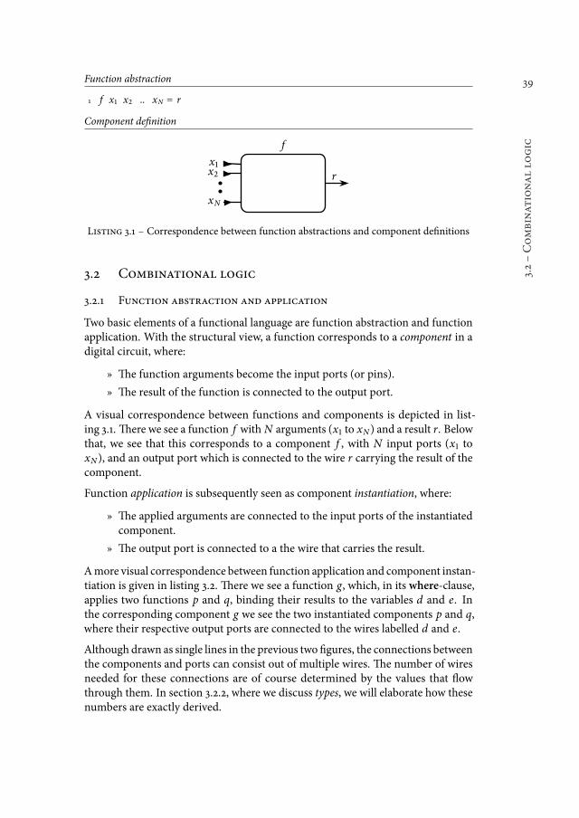
39

3.2śCombinat

ionallo

gic

Function abstraction

1 f x1 x2 .. xN = r

Component deinition

f

x�x�

xN

r

Listing 3.1 ś Correspondence between function abstractions and component deinitions

3.2 Combinational logic

3.2.1 Function abstraction and application

Two basic elements of a functional language are function abstraction and functionapplication. With the structural view, a function corresponds to a component in adigital circuit, where:

ż he function arguments become the input ports (or pins).

ż he result of the function is connected to the output port.

A visual correspondence between functions and components is depicted in list-ing 3.1. here we see a function f with N arguments (x1 to xN ) and a result r. Belowthat, we see that this corresponds to a component f , with N input ports (x1 toxN ), and an output port which is connected to the wire r carrying the result of thecomponent.

Function application is subsequently seen as component instantiation, where:

ż he applied arguments are connected to the input ports of the instantiatedcomponent.

ż he output port is connected to a the wire that carries the result.

Amore visual correspondence between function application and component instan-tiation is given in listing 3.2. here we see a function g, which, in its where-clause,applies two functions p and q, binding their results to the variables d and e. Inthe corresponding component g we see the two instantiated components p and q,where their respective output ports are connected to the wires labelled d and e.

Although drawn as single lines in the previous two igures, the connections betweenthe components and ports can consist out of multiple wires. he number of wiresneeded for these connections are of course determined by the values that lowthrough them. In section 3.2.2, where we discuss types, we will elaborate how thesenumbers are exactly derived.

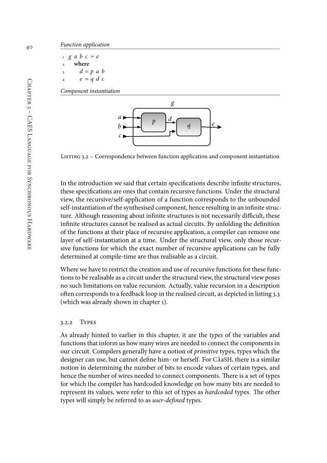
40

Chapter

3śCAESLanguagefo

rSynchronousHardware

Function application

1 g a b c = e2 where

3 d = p a b4 e = q d c

Component instantiation

g

a

b

c

ep

qd

Listing 3.2 ś Correspondence between function application and component instantiation

In the introduction we said that certain speciications describe ininite structures,these speciications are ones that contain recursive functions. Under the structuralview, the recursive/self-application of a function corresponds to the unboundedself-instantiation of the synthesised component, hence resulting in an ininite struc-ture. Although reasoning about ininite structures is not necessarily diicult, theseininite structures cannot be realised as actual circuits. By unfolding the deinitionof the functions at their place of recursive application, a compiler can remove onelayer of self-instantiation at a time. Under the structural view, only those recur-sive functions for which the exact number of recursive applications can be fullydetermined at compile-time are thus realisable as a circuit.

Where we have to restrict the creation and use of recursive functions for these func-tions to be realisable as a circuit under the structural view, the structural view posesno such limitations on value recursion. Actually, value recursion in a descriptionoten corresponds to a feedback loop in the realised circuit, as depicted in listing 3.3(which was already shown in chapter 1).

3.2.2 Types

As already hinted to earlier in this chapter, it are the types of the variables andfunctions that inform us howmany wires are needed to connect the components inour circuit. Compilers generally have a notion of primitive types, types which thedesigner can use, but cannot deine him- or herself. For CλaSH, there is a similarnotion in determining the number of bits to encode values of certain types, andhence the number of wires needed to connect components. here is a set of typesfor which the compiler has hardcoded knowledge on how many bits are needed torepresent its values, were refer to this set of types as hardcoded types. he othertypes will simply be referred to as user-deined types.

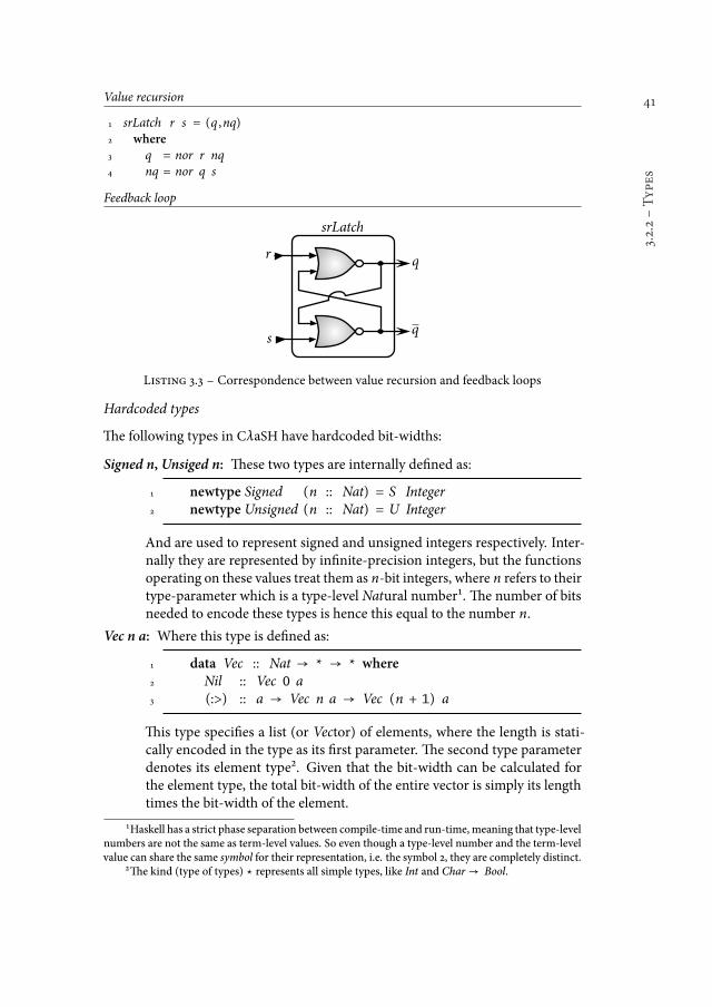
41

3.2.2śTypes

Value recursion

1 srLatch r s = (q ,nq)2 where

3 q = nor r nq4 nq = nor q s

Feedback loop

s

rq

q

srLatch

Listing 3.3 ś Correspondence between value recursion and feedback loops

Hardcoded types

he following types in CλaSH have hardcoded bit-widths:

Signed n, Unsiged n: hese two types are internally deined as:

1 newtype Signed (n :: Nat) = S Integer2 newtype Unsigned (n :: Nat) = U Integer

And are used to represent signed and unsigned integers respectively. Inter-nally they are represented by ininite-precision integers, but the functionsoperating on these values treat them as n-bit integers, where n refers to theirtype-parameter which is a type-level Natural number¹. he number of bitsneeded to encode these types is hence this equal to the number n.

Vec n a: Where this type is deined as:

1 data Vec :: Nat → * → * where2 Nil :: Vec 0 a3 (:>) :: a → Vec n a → Vec (n + 1) a

his type speciies a list (or Vector) of elements, where the length is stati-cally encoded in the type as its irst parameter. he second type parameterdenotes its element type². Given that the bit-width can be calculated forthe element type, the total bit-width of the entire vector is simply its lengthtimes the bit-width of the element.

1Haskell has a strict phase separation between compile-time and run-time, meaning that type-levelnumbers are not the same as term-level values. So even though a type-level number and the term-levelvalue can share the same symbol for their representation, i.e. the symbol 2, they are completely distinct.

2he kind (type of types) ⋆ represents all simple types, like Int and Char→ Bool.

42

Chapter

3śCAESLanguagefo

rSynchronousHardware

User-deined types

A designer may deine a completely new type by using the data keyword. hefollowing algebraic types have a fully determinable bit-width:

Product types: A product type has a single constructor which has multiple ields,such as tuples, and record types. An example of a product type would be:

1 data Enabled a = Enabled Bool a

Which has one constructor, Enabled, and two ields: one of type Bool andone with the type of the type parameter a. he bit-width of a product typeis simply the sum of the bit-width of the types of its ields.

Simple sum types (enumerations): Simple sum types, or enumerations, have mul-tiple constructors, but where the constructors have no ields. A well knownenumeration is the Boolean type:

1 data Bool = False | True

he bit-width for these types is: ⌈log2 c⌉, where c is the number of construc-tors.

Sum types: Sum types (sometimes called sum-of-product types to diferentiatefrom simple sum types) have multiple constructors, where the constructorscan have multiple ields. A well know sum type is the Either type:

1 data Either a b = Let a | Right b

Which has two constructors, and each constructor has one ield. he bit-width of a sum type is calculated by:

1. For every constructor: sum the bit-width of their respective ields.

2. Calculate the maximum of these sums.

3. Add ⌈log2 c⌉, where c is the number of constructors.

Recursively deined types can, in general, not be given a ixed bit-width: it usuallynot possible to determine how many times a recursive type can be unfolded. hatis also the main reason why the Vector type has a hard-coded bit-width calculation.However, the very fact that there is a hard-coded calculation indicates that it isnot impossible to determine the bit-width for certain recursive types. For Vectors,the size can be fully determined due to the fact that it has a natural number as atype-parameter which restricts both which and how many of its constructors mustbe used to create a valid value. Generalising such an analysis to other recursivedata types is considered future work.

3.2.3 Choice

In Haskell, choice can be achieved by a large set of syntactic elements, consisting of:case expressions, if−then−else expressions, multiple-clause function deinitions,

43

3.2.3śChoice

and guards. he most general of these are the (pattern-matching) case expressions:all others forms of choice can be translated to case expressions. We hence use thecircuit interpretation for case expressions as the circuit interpretation for all choiceconstructs.

In general, a case expression is of the form:

1 case subject of2 C1 x1 .. xM → alternative13 ..4 CN y1 .. yK → alternativeN

Where an alternative is chosen based on the constructor shape (C1 ..CN ) of thesubject. Aside from choosing an alternative, the case expressions also binds theields corresponding to the constructor to variables (x1 ..xM), which can be usedin the selected alternative. hese two aspects of case-expressions, selection andprojection, have separate circuit interpretations.

We start with the interpretation for selection. he structural view on the selectionaspect gives us amultiplexer, where:

ż he wires representing the constructor part of the subject are connected tothe selection port.

ż he result of the alternatives are connected to the input ports.

For the synthesis of expressions to circuits we assume that all the functions that wewill be working with are side-efect free, which is an aspect that can be staticallyasserted inHaskell. When the expressions in the alternatives are side-efect free, theparallel calculations happening in the eventual circuit will not interfere with eachother. he observed behaviour of the complete circuit, of what in sotware termswould be called łspeculativež parallel execution, is hence faithful to the semanticsof the case-expression³.

Two, semantically equal but syntactically distinct, code examples of a counter cir-cuit, and the circuit interpretation that corresponds to both speciications, are givenin listing 3.4. he function counts up or down depending on the direction variable,and has a wrap variable that determines the wrap-around point of the counter.

he other aspect of case expressions, aside from selection, is binding the values ofconstructor ields to variables. his aspect is called projection. Given that a valueof a data type with ields travels over N wires, projection is simply continuing withM of these wires that represent the ield. Listing 3.5 demonstrates this projectionaspect of case expressions and the corresponding circuit interpretation for a simpleproduct type. In this igure we mark the bit-width (in the form of bit-indices) ofthe individual wires to get a better understanding of the circuit interpretation forprojection.

3Assuming no alternative evaluates to bottom, which also would not have a circuit representation.

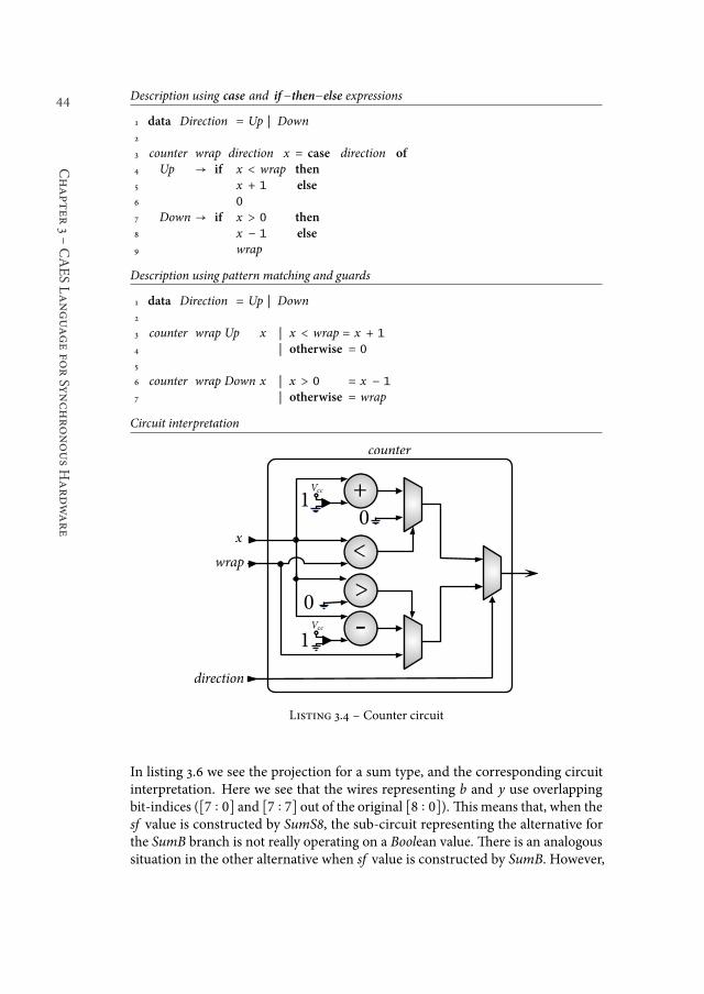
44

Chapter

3śCAESLanguagefo

rSynchronousHardware

Description using case and if−then−else expressions

1 data Direction = Up | Down2

3 counter wrap direction x = case direction of

4 Up → if x < wrap then

5 x + 1 else

6 0

7 Down → if x > 0 then

8 x − 1 else

9 wrap

Description using pattern matching and guards

1 data Direction = Up | Down2

3 counter wrap Up x | x < wrap = x + 1

4 | otherwise = 0

5

6 counter wrap Down x | x > 0 = x − 1

7 | otherwise = wrap

Circuit interpretation

x

wrap

direction

+

counter

�

�

<

-

>

�

�

Vcc

Vcc

Listing 3.4 ś Counter circuit

In listing 3.6 we see the projection for a sum type, and the corresponding circuitinterpretation. Here we see that the wires representing b and y use overlappingbit-indices (∥7 ∶ 0∥ and ∥7 ∶ 7∥ out of the original ∥8 ∶ 0∥). his means that, when thesf value is constructed by SumS8, the sub-circuit representing the alternative forthe SumB branch is not really operating on a Boolean value. here is an analogoussituation in the other alternative when sf value is constructed by SumB. However,

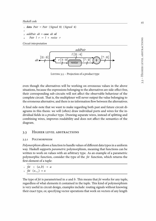
45

3.3śHigher

level

abstractions

Haskell code

1 data Pair = Pair (Signed 8) (Signed 4)2

3 addPair ab = case ab of

4 Pair l r → l + resize r

Circuit interpretation

ab +

addPair

[�� ∶ �][�� ∶ �]

[� ∶ �]resize

[� ∶ �][� ∶ �]

l

r

Listing 3.5 ś Projection of a product type

even though the alternatives will be working on erroneous values in the abovesituations, because the expressions belonging to the alternatives are side-efect free,their corresponding sub-circuits will not afect the observable behaviour of thecomplete circuit. hat is, the multiplexer will never output the value belonging tothe erroneous alternative, and there is no information low between the alternatives.

A inal side-note that we want to make regarding both past and future circuit di-agrams in this thesis: we will (oten) draw individual ports and wires for the in-dividual ields in a product type. Drawing separate wires, instead of splitting andcombining wires, improves readability and does not afect the semantics of thediagram.

3.3 Higher level abstractions

3.3.1 Polymorphism

Polymorphism allows a function to handle values of diferent data types in a uniformway. Haskell supports parametric polymorphism, meaning that functions can bewritten to work on values with an arbitrary type. As an example of a parametricpolymorphic function, consider the type of the fst function, which returns theirst element of a tuple:

1 fst :: (a ,b) → a2 fst (x ,_) = x

he type of fst is parametrised in a and b. his means that fst works for any tuple,regardless of what elements it contained in the tuple. his kind of polymorphismis very useful in circuit design, examples include: routing signals without knowingtheir exact type, or, specifying vector operations that work on vectors of any length

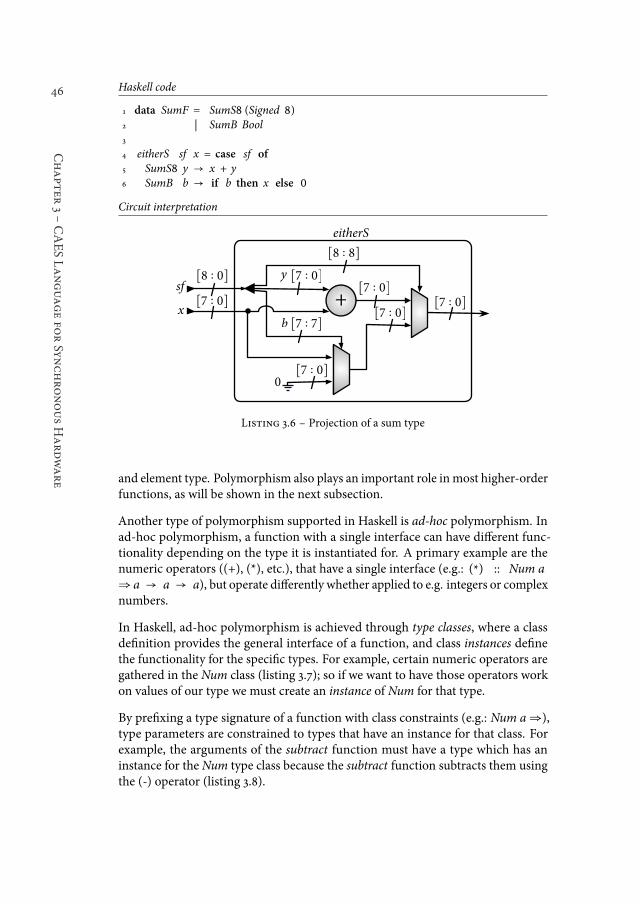
46

Chapter

3śCAESLanguagefo

rSynchronousHardware

Haskell code

1 data SumF = SumS8 (Signed 8)2 | SumB Bool3

4 eitherS sf x = case sf of

5 SumS8 y → x + y6 SumB b → if b then x else 0

Circuit interpretation

sf+

eitherS

[� ∶ �]

[� ∶ �]

[� ∶ �]

[� ∶ �]

[� ∶ �][� ∶ �]

[� ∶ �][� ∶ �]

[� ∶ �]�

x

y

b

Listing 3.6 ś Projection of a sum type

and element type. Polymorphism also plays an important role inmost higher-orderfunctions, as will be shown in the next subsection.

Another type of polymorphism supported in Haskell is ad-hoc polymorphism. Inad-hoc polymorphism, a function with a single interface can have diferent func-tionality depending on the type it is instantiated for. A primary example are thenumeric operators ((+), (*), etc.), that have a single interface (e.g.: (*) :: Num a⇒ a → a → a), but operate diferently whether applied to e.g. integers or complexnumbers.

In Haskell, ad-hoc polymorphism is achieved through type classes, where a classdeinition provides the general interface of a function, and class instances deinethe functionality for the speciic types. For example, certain numeric operators aregathered in the Num class (listing 3.7); so if we want to have those operators workon values of our type we must create an instance of Num for that type.

By preixing a type signature of a function with class constraints (e.g.: Num a⇒),type parameters are constrained to types that have an instance for that class. Forexample, the arguments of the subtract function must have a type which has aninstance for the Num type class because the subtract function subtracts them usingthe (-) operator (listing 3.8).

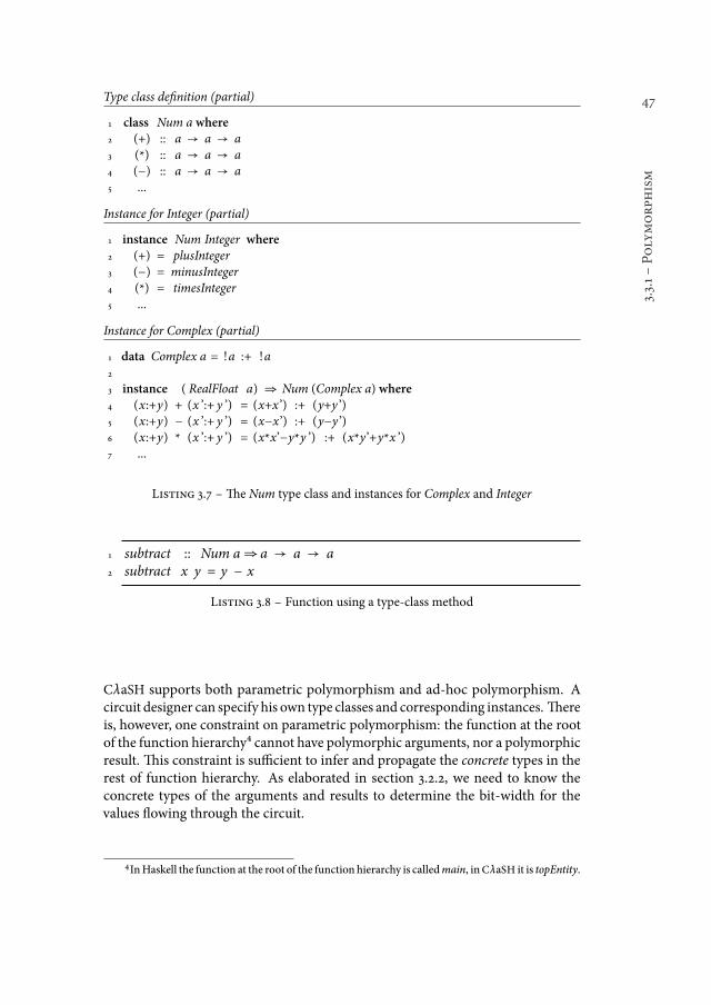
47

3.3.1śPolymorph

ism

Type class deinition (partial)

1 class Num a where2 (+) :: a → a → a3 (*) :: a → a → a4 (−) :: a → a → a5 ...

Instance for Integer (partial)

1 instance Num Integer where

2 (+) = plusInteger3 (−) = minusInteger4 (*) = timesInteger5 ...

Instance for Complex (partial)

1 data Complex a = !a :+ !a2

3 instance ( RealFloat a) ⇒ Num (Complex a) where4 (x:+y) + (x ’:+ y ’) = (x+x ’) :+ (y+y ’)5 (x:+y) − (x ’:+ y ’) = (x−x’) :+ (y−y ’)6 (x:+y) * (x ’:+ y ’) = (x*x’−y*y ’) :+ (x*y’+y*x ’)7 ...

Listing 3.7 ś he Num type class and instances for Complex and Integer

1 subtract :: Num a⇒ a → a → a2 subtract x y = y − x

Listing 3.8 ś Function using a type-class method

CλaSH supports both parametric polymorphism and ad-hoc polymorphism. Acircuit designer can specify his own type classes and corresponding instances. hereis, however, one constraint on parametric polymorphism: the function at the rootof the function hierarchy4 cannot have polymorphic arguments, nor a polymorphicresult. his constraint is suicient to infer and propagate the concrete types in therest of function hierarchy. As elaborated in section 3.2.2, we need to know theconcrete types of the arguments and results to determine the bit-width for thevalues lowing through the circuit.

4InHaskell the function at the root of the function hierarchy is calledmain, inCλaSH it is topEntity.

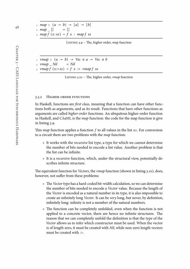
48

Chapter

3śCAESLanguagefo

rSynchronousHardware

1 map :: (a → b) → [a] → [b]2 map _ [] = []3 map f (x : xs) = f x : map f xs

Listing 3.9 ś he, higher order,map function

1 vmap :: (a → b) → Vec n a → Vec n b2 vmap _ Nil = Nil3 vmap f (x:>xs) = f x :> vmap f xs

Listing 3.10 ś he, higher order, vmap function

3.3.2 Higher-order functions

In Haskell, functions are irst class, meaning that a function can have other func-tions both as arguments, and as its result. Functions that have other functions asarguments are called higher-order functions. An ubiquitous higher-order functionin Haskell, and CλaSH, is themap function: the code for the map function is givein listing 3.9.

his map function applies a function f to all values in the list xs. For conversionto a circuit there are two problems with themap function:

ż It works with the recursive list type, a type for which we cannot determinethe number of bits needed to encode a list value. Another problem is thatthe list can be ininite.

ż It is a recursive function, which, under the structural view, potentially de-scribes ininite structure.

he equivalent function forVectors, the vmap function (shown in listing 3.10), does,however, not sufer from these problems:

ż heVector type has a hard-coded bit-width calculation, so we can determinethe number of bits needed to encode a Vector value. Because the length ofthe Vector is encoded as a natural number in its type, it is also impossible tocreate an ininitely long Vector. It can be very long, but never, by deinition,ininitely long: ininity is not a member of the natural numbers.

ż he function can be completely unfolded, even when the function is notapplied to a concrete vector, there are hence no ininite structures. hereason that we can completely unfold the deinition is that the type of theVector allows us to infer which constructor must be used. When the vectoris of length zero, it must be created with Nil, while non-zero length vectorsmust be created with :>.

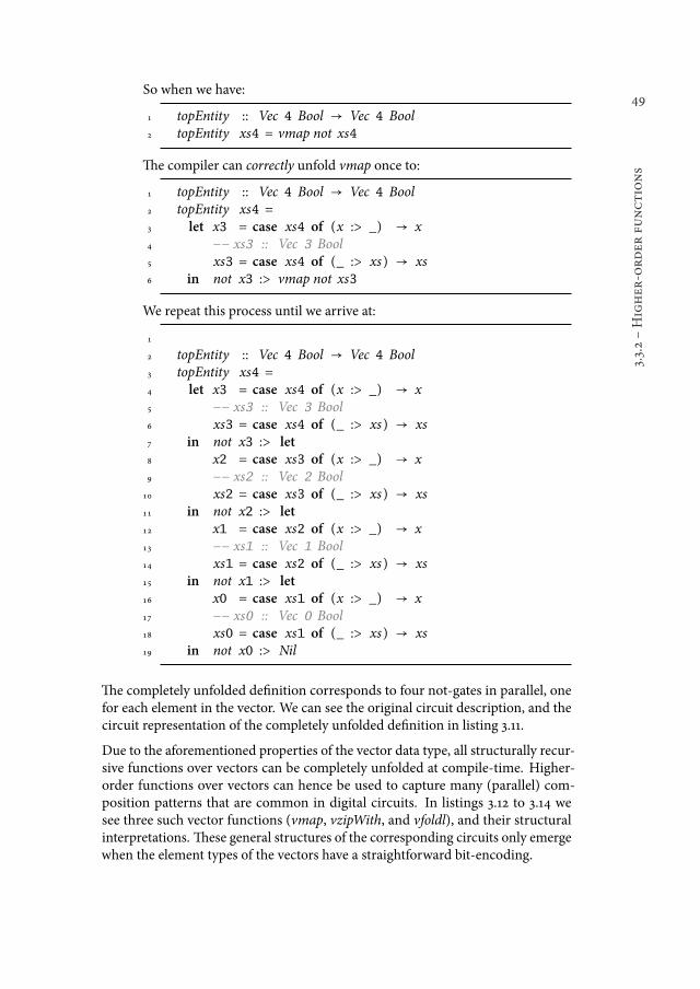
49

3.3.2śHigher

-order

functions

So when we have:

1 topEntity :: Vec 4 Bool → Vec 4 Bool2 topEntity xs4 = vmap not xs4

he compiler can correctly unfold vmap once to:

1 topEntity :: Vec 4 Bool → Vec 4 Bool2 topEntity xs4 =3 let x3 = case xs4 of (x :> _) → x4 −− xs3 :: Vec 3 Bool5 xs3 = case xs4 of (_ :> xs) → xs6 in not x3 :> vmap not xs3

We repeat this process until we arrive at:

1

2 topEntity :: Vec 4 Bool → Vec 4 Bool3 topEntity xs4 =4 let x3 = case xs4 of (x :> _) → x5 −− xs3 :: Vec 3 Bool6 xs3 = case xs4 of (_ :> xs) → xs7 in not x3 :> let8 x2 = case xs3 of (x :> _) → x9 −− xs2 :: Vec 2 Bool

10 xs2 = case xs3 of (_ :> xs) → xs11 in not x2 :> let12 x1 = case xs2 of (x :> _) → x13 −− xs1 :: Vec 1 Bool14 xs1 = case xs2 of (_ :> xs) → xs15 in not x1 :> let16 x0 = case xs1 of (x :> _) → x17 −− xs0 :: Vec 0 Bool18 xs0 = case xs1 of (_ :> xs) → xs19 in not x0 :> Nil

he completely unfolded deinition corresponds to four not-gates in parallel, onefor each element in the vector. We can see the original circuit description, and thecircuit representation of the completely unfolded deinition in listing 3.11.

Due to the aforementioned properties of the vector data type, all structurally recur-sive functions over vectors can be completely unfolded at compile-time. Higher-order functions over vectors can hence be used to capture many (parallel) com-position patterns that are common in digital circuits. In listings 3.12 to 3.14 wesee three such vector functions (vmap, vzipWith, and vfoldl), and their structuralinterpretations. hese general structures of the corresponding circuits only emergewhen the element types of the vectors have a straightforward bit-encoding.

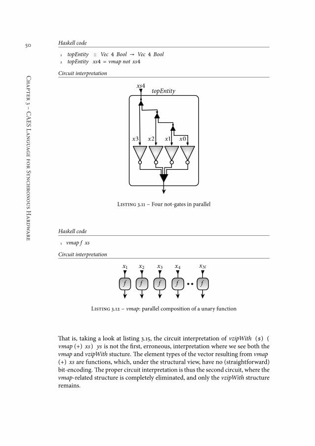
50

Chapter

3śCAESLanguagefo

rSynchronousHardware

Haskell code

1 topEntity :: Vec 4 Bool → Vec 4 Bool2 topEntity xs4 = vmap not xs4

Circuit interpretation

x�

xs�

x� x�

topEntity

x�

Listing 3.11 ś Four not-gates in parallel

Haskell code

1 vmap f xs

Circuit interpretation

xNx�x�

f

x� x�

f f f f

Listing 3.12 ś vmap: parallel composition of a unary function

hat is, taking a look at listing 3.15, the circuit interpretation of vzipWith ($) (vmap (+) xs) ys is not the irst, erroneous, interpretation where we see both thevmap and vzipWith stucture. he element types of the vector resulting from vmap(+) xs are functions, which, under the structural view, have no (straightforward)bit-encoding. he proper circuit interpretation is thus the second circuit, where thevmap-related structure is completely eliminated, and only the vzipWith structureremains.

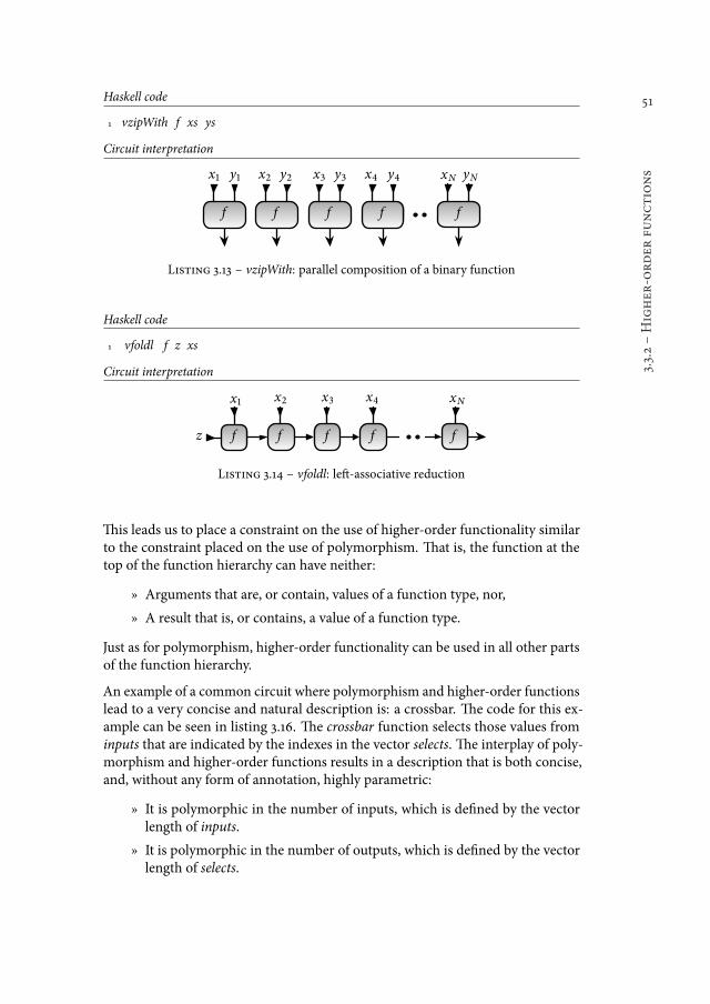
51

3.3.2śHigher

-order

functions

Haskell code

1 vzipWith f xs ys

Circuit interpretation

xNx�x�

f

y� y� yNx�x� y� y�

f f f f

Listing 3.13 ś vzipWith: parallel composition of a binary function

Haskell code

1 vfoldl f z xs

Circuit interpretation

xNx�x�

f f fz f f

x� x�

Listing 3.14 ś vfoldl: let-associative reduction

his leads us to place a constraint on the use of higher-order functionality similarto the constraint placed on the use of polymorphism. hat is, the function at thetop of the function hierarchy can have neither:

ż Arguments that are, or contain, values of a function type, nor,

ż A result that is, or contains, a value of a function type.

Just as for polymorphism, higher-order functionality can be used in all other partsof the function hierarchy.

An example of a common circuit where polymorphism and higher-order functionslead to a very concise and natural description is: a crossbar. he code for this ex-ample can be seen in listing 3.16. he crossbar function selects those values frominputs that are indicated by the indexes in the vector selects. he interplay of poly-morphism and higher-order functions results in a description that is both concise,and, without any form of annotation, highly parametric:

ż It is polymorphic in the number of inputs, which is deined by the vectorlength of inputs.

ż It is polymorphic in the number of outputs, which is deined by the vectorlength of selects.

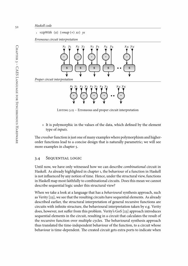
52

Chapter

3śCAESLanguagefo

rSynchronousHardware

Haskell code

1 vzipWith ($) (vmap (+) xs) ys

Erroneous circuit interpretation

xNx�x�

�

y� y� yNx�x� y� y�

+

�

+

�

+

�

+

�

+

Proper circuit interpretation

xNx�x� y� y� yNx�x� y� y�

+ + + + +

Listing 3.15 ś Erroneous and proper circuit interpretation

ż It is polymorphic in the values of the data, which deined by the elementtype of inputs.

he crossbar function is just one ofmany exampleswhere polymorphismandhigher-order functions lead to a concise design that is naturally parametric; we will seemore examples in chapter 5.

3.4 Sequential logic

Until now, we have only witnessed how we can describe combinational circuit inHaskell. As already highlighted in chapter 1, the behaviour of a function in Haskellis not inluenced by any notion of time. Hence, under the structural view, functionsin Haskell mapmost faithfully to combinational circuits. Does this mean we cannotdescribe sequential logic under this structural view?

When we take a look at a language that has a behavioural synthesis approach, suchas Verity [23], we see that the resulting circuits have sequential elements. As alreadydescribed earlier, the structural interpretation of general recursive functions arecircuits with ininite structure, the behavioural interpretation taken by e.g. Veritydoes, however, not sufer from this problem. Verity’s GoS [23] approach introducessequential elements in the circuit, resulting in a circuit that calculates the result ofthe recursive function over multiple cycles. he behavioural synthesis approachthus translated the time-independent behaviour of the function, to a circuit whosebehaviour is time-dependent. he created circuit gets extra ports to indicate when

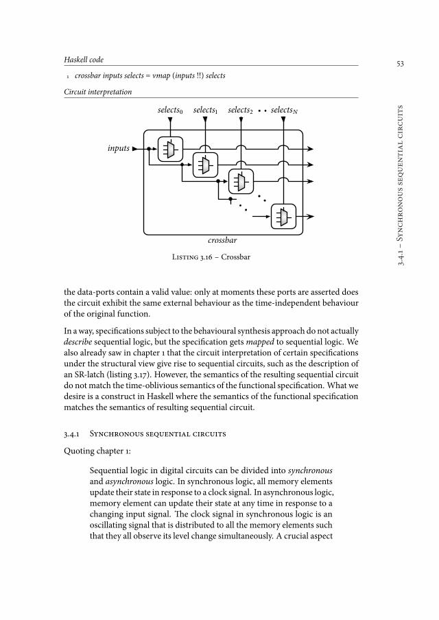
53

3.4.1śSynchronoussequen

tialcircuits

Haskell code

1 crossbar inputs selects = vmap (inputs !!) selects

Circuit interpretation

inputs

selects�

crossbar

selects� selects� selectsN

Listing 3.16 ś Crossbar

the data-ports contain a valid value: only at moments these ports are asserted doesthe circuit exhibit the same external behaviour as the time-independent behaviourof the original function.

In away, speciications subject to the behavioural synthesis approach do not actuallydescribe sequential logic, but the speciication getsmapped to sequential logic. Wealso already saw in chapter 1 that the circuit interpretation of certain speciicationsunder the structural view give rise to sequential circuits, such as the description ofan SR-latch (listing 3.17). However, the semantics of the resulting sequential circuitdo notmatch the time-oblivious semantics of the functional speciication. What wedesire is a construct in Haskell where the semantics of the functional speciicationmatches the semantics of resulting sequential circuit.

3.4.1 Synchronous sequential circuits

Quoting chapter 1:

Sequential logic in digital circuits can be divided into synchronousand asynchronous logic. In synchronous logic, all memory elementsupdate their state in response to a clock signal. In asynchronous logic,memory element can update their state at any time in response to achanging input signal. he clock signal in synchronous logic is anoscillating signal that is distributed to all the memory elements suchthat they all observe its level change simultaneously. A crucial aspect

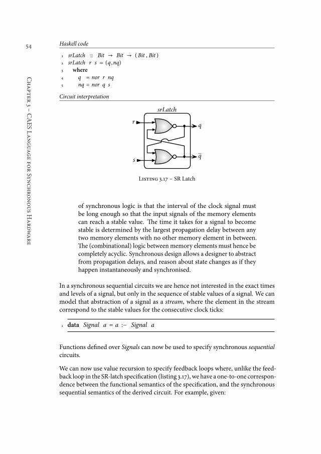
54

Chapter

3śCAESLanguagefo

rSynchronousHardware

Haskell code

1 srLatch :: Bit → Bit → (Bit , Bit )2 srLatch r s = (q ,nq)3 where

4 q = nor r nq5 nq = nor q s

Circuit interpretation

s

rq

q

srLatch

Listing 3.17 ś SR Latch

of synchronous logic is that the interval of the clock signal mustbe long enough so that the input signals of the memory elementscan reach a stable value. he time it takes for a signal to becomestable is determined by the largest propagation delay between anytwo memory elements with no other memory element in between.he (combinational) logic betweenmemory elements must hence becompletely acyclic. Synchronous design allows a designer to abstractfrom propagation delays, and reason about state changes as if theyhappen instantaneously and synchronised.

In a synchronous sequential circuits we are hence not interested in the exact timesand levels of a signal, but only in the sequence of stable values of a signal. We canmodel that abstraction of a signal as a stream, where the element in the streamcorrespond to the stable values for the consecutive clock ticks:

1 data Signal a = a :− Signal a

Functions deined over Signals can now be used to specify synchronous sequentialcircuits.

We can now use value recursion to specify feedback loops where, unlike the feed-back loop in the SR-latch speciication (listing 3.17), we have a one-to-one correspon-dence between the functional semantics of the speciication, and the synchronoussequential semantics of the derived circuit. For example, given:

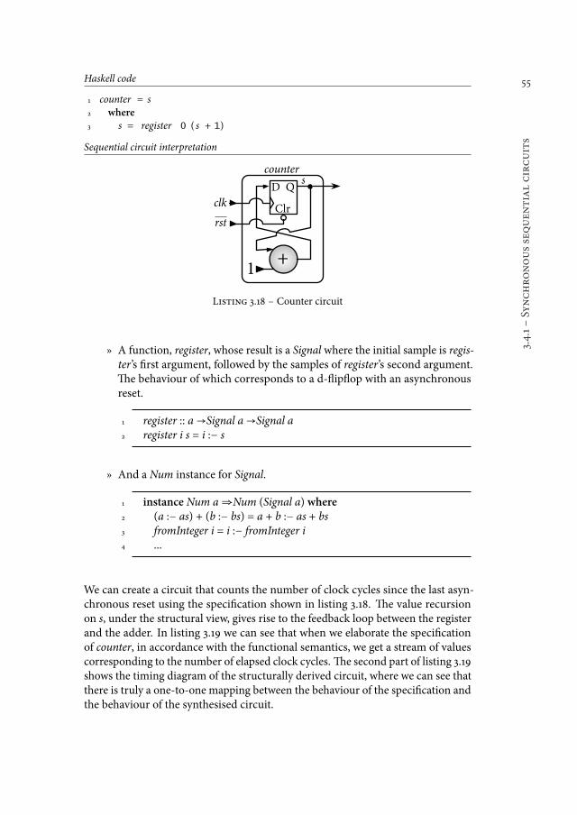
55

3.4.1śSynchronoussequen

tialcircuits

Haskell code

1 counter = s2 where

3 s = register 0 ( s + 1)

Sequential circuit interpretation

rst

clk

+

counter

�

D Q

Clr

s

Listing 3.18 ś Counter circuit

ż A function, register, whose result is a Signal where the initial sample is regis-ter’s irst argument, followed by the samples of register’s second argument.he behaviour of which corresponds to a d-liplop with an asynchronousreset.

1 register :: a→Signal a→Signal a2 register i s = i :− s

ż And a Num instance for Signal.

1 instance Num a⇒Num (Signal a) where2 (a :− as) + (b :− bs) = a + b :− as + bs3 fromInteger i = i :− fromInteger i4 ...

We can create a circuit that counts the number of clock cycles since the last asyn-chronous reset using the speciication shown in listing 3.18. he value recursionon s, under the structural view, gives rise to the feedback loop between the registerand the adder. In listing 3.19 we can see that when we elaborate the speciicationof counter, in accordance with the functional semantics, we get a stream of valuescorresponding to the number of elapsed clock cycles. he second part of listing 3.19shows the timing diagram of the structurally derived circuit, where we can see thatthere is truly a one-to-one mapping between the behaviour of the speciication andthe behaviour of the synthesised circuit.

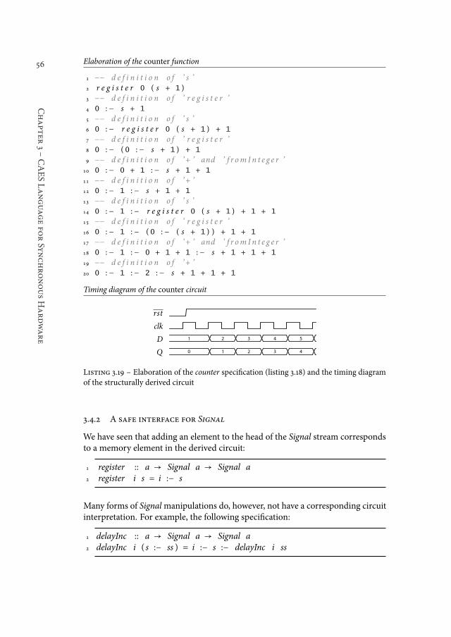
56

Chapter

3śCAESLanguagefo

rSynchronousHardware

Elaboration of the counter function

1 −− d e f i n i t i o n o f ’ s ’2 r e g i s t e r 0 ( s + 1 )3 −− d e f i n i t i o n o f ’ r e g i s t e r ’4 0 :− s + 1

5 −− d e f i n i t i o n o f ’ s ’6 0 :− r e g i s t e r 0 ( s + 1 ) + 1

7 −− d e f i n i t i o n o f ’ r e g i s t e r ’8 0 :− ( 0 :− s + 1 ) + 1

9 −− d e f i n i t i o n o f ’+ ’ and ’ f r om I n t e g e r ’10 0 :− 0 + 1 :− s + 1 + 1

11 −− d e f i n i t i o n o f ’+ ’12 0 :− 1 :− s + 1 + 1

13 −− d e f i n i t i o n o f ’ s ’14 0 :− 1 :− r e g i s t e r 0 ( s + 1 ) + 1 + 1

15 −− d e f i n i t i o n o f ’ r e g i s t e r ’16 0 :− 1 :− ( 0 :− ( s + 1 ) ) + 1 + 1

17 −− d e f i n i t i o n o f ’+ ’ and ’ f r om I n t e g e r ’18 0 :− 1 :− 0 + 1 + 1 :− s + 1 + 1 + 1

19 −− d e f i n i t i o n o f ’+ ’20 0 :− 1 :− 2 :− s + 1 + 1 + 1

Timing diagram of the counter circuit

rst

clk

D 1 2 3 4 5

Q 0 1 2 3 4

Listing 3.19 ś Elaboration of the counter speciication (listing 3.18) and the timing diagramof the structurally derived circuit

3.4.2 A safe interface for Signal

We have seen that adding an element to the head of the Signal stream correspondsto a memory element in the derived circuit:

1 register :: a → Signal a → Signal a2 register i s = i :− s

Many forms of Signalmanipulations do, however, not have a corresponding circuitinterpretation. For example, the following speciication:

1 delayInc :: a → Signal a → Signal a2 delayInc i ( s :− ss ) = i :− s :− delayInc i ss

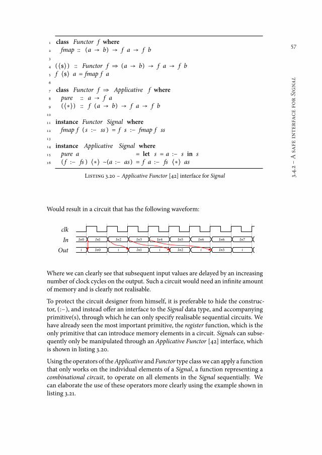
57

3.4.2śAsafe

interfacefo

rSignal

1 class Functor f where2 fmap :: (a → b) → f a → f b3

4 (⟨$⟩) :: Functor f ⇒ (a → b) → f a → f b5 f ⟨$⟩ a = fmap f a6

7 class Functor f ⇒ Applicative f where8 pure :: a → f a9 (⟨∗⟩) :: f (a → b) → f a → f b

10

11 instance Functor Signal where12 fmap f ( s :− ss ) = f s :− fmap f ss13

14 instance Applicative Signal where15 pure a = let s = a :− s in s16 ( f :− fs ) ⟨∗⟩ ~(a :− as) = f a :− fs ⟨∗⟩ as

Listing 3.20 ś Applicative Functor [42] interface for Signal

Would result in a circuit that has the following waveform:

clk

In In0 In1 In2 In3 In4 In5 In6 In6 In7

Out i In0 i In1 i In2 i In3 i

Where we can clearly see that subsequent input values are delayed by an increasingnumber of clock cycles on the output. Such a circuit would need an ininite amountof memory and is clearly not realisable.

To protect the circuit designer from himself, it is preferable to hide the construc-tor, (:−), and instead ofer an interface to the Signal data type, and accompanyingprimitive(s), through which he can only specify realisable sequential circuits. Wehave already seen the most important primitive, the register function, which is theonly primitive that can introduce memory elements in a circuit. Signals can subse-quently only be manipulated through an Applicative Functor [42] interface, whichis shown in listing 3.20.

Using the operators of theApplicative and Functor type class we can apply a functionthat only works on the individual elements of a Signal, a function representing acombinational circuit, to operate on all elements in the Signal sequentially. Wecan elaborate the use of these operators more clearly using the example shown inlisting 3.21.

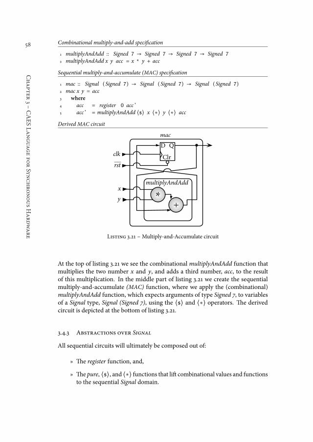
58

Chapter

3śCAESLanguagefo

rSynchronousHardware

Combinational multiply-and-add speciication

1 multiplyAndAdd :: Signed 7 → Signed 7 → Signed 7 → Signed 7

2 multiplyAndAdd x y acc = x * y + acc

Sequential multiply-and-accumulate (MAC) speciication

1 mac :: Signal (Signed 7) → Signal (Signed 7) → Signal (Signed 7)2 mac x y = acc3 where

4 acc = register 0 acc ’5 acc ’ = multiplyAndAdd ⟨$⟩ x ⟨∗⟩ y ⟨∗⟩ acc

DerivedMAC circuit

rst

clk

mac

x

D Q

Clr

multiplyAndAdd

y∗

+

Listing 3.21 ś Multiply-and-Accumulate circuit

At the top of listing 3.21 we see the combinational multiplyAndAdd function thatmultiplies the two number x and y, and adds a third number, acc, to the resultof this multiplication. In the middle part of listing 3.21 we create the sequentialmultiply-and-accumulate (MAC) function, where we apply the (combinational)multiplyAndAdd function, which expects arguments of type Signed 7, to variablesof a Signal type, Signal (Signed 7), using the ⟨$⟩ and ⟨∗⟩ operators. he derivedcircuit is depicted at the bottom of listing 3.21.

3.4.3 Abstractions over Signal

All sequential circuits will ultimately be composed out of:

ż he register function, and,

ż he pure, ⟨$⟩, and ⟨∗⟩ functions that lit combinational values and functionsto the sequential Signal domain.

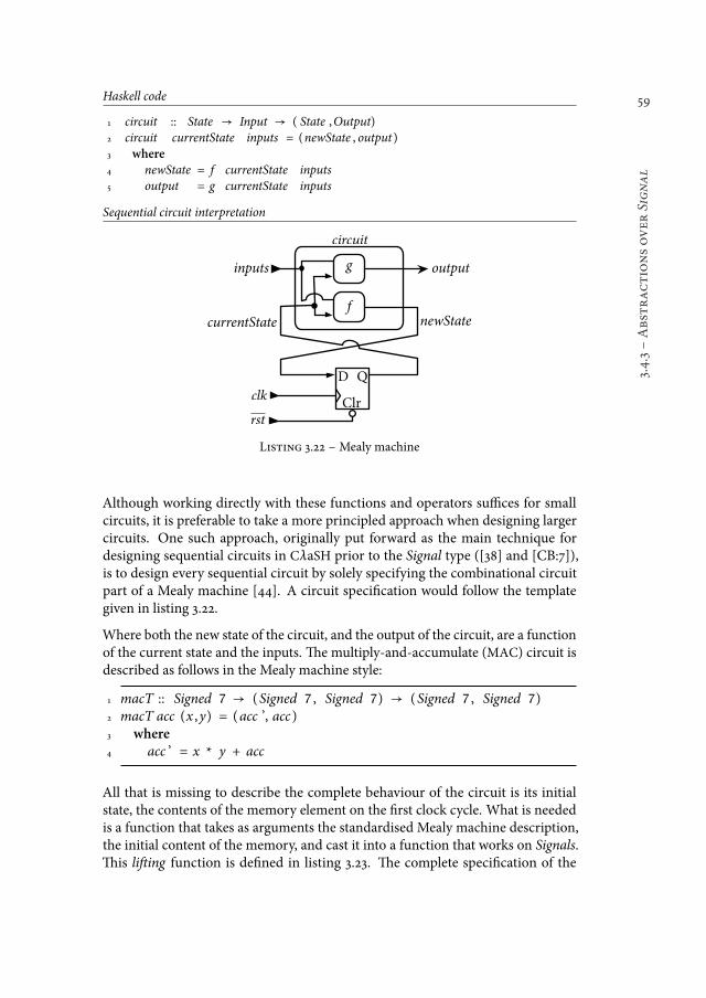
59

3.4.3śAbstractionsover

Signal

Haskell code

1 circuit :: State → Input → ( State ,Output)2 circuit currentState inputs = (newState , output )3 where

4 newState = f currentState inputs5 output = g currentState inputs

Sequential circuit interpretation

rst

clk

inputs

D Q

Clr

circuit

g

fcurrentState newState

output

Listing 3.22 ś Mealy machine

Although working directly with these functions and operators suices for smallcircuits, it is preferable to take a more principled approach when designing largercircuits. One such approach, originally put forward as the main technique fordesigning sequential circuits in CλaSH prior to the Signal type ([38] and [CB:7]),is to design every sequential circuit by solely specifying the combinational circuitpart of a Mealy machine [44]. A circuit speciication would follow the templategiven in listing 3.22.

Where both the new state of the circuit, and the output of the circuit, are a functionof the current state and the inputs. he multiply-and-accumulate (MAC) circuit isdescribed as follows in the Mealy machine style:

1 macT :: Signed 7 → (Signed 7 , Signed 7) → (Signed 7 , Signed 7)2 macT acc (x ,y) = (acc ’, acc )3 where4 acc ’ = x * y + acc

All that is missing to describe the complete behaviour of the circuit is its initialstate, the contents of the memory element on the irst clock cycle. What is neededis a function that takes as arguments the standardised Mealy machine description,the initial content of the memory, and cast it into a function that works on Signals.his liting function is deined in listing 3.23. he complete speciication of the

60

Chapter

3śCAESLanguagefo

rSynchronousHardware

1 (⟨^⟩) :: ( s → i → ( s ,o)) → s → ( Signal i → Signal o)2 mealyT ⟨^⟩ initS =3 λinp → let r = register initS ( fst ⟨$⟩ outp)4 outp = mealyT ⟨$⟩ r ⟨∗⟩ inp5 in snd ⟨$⟩ outp

Listing 3.23 ś Creating Mealy machines

1 (⟨^⟩) :: ( s → i → ( s ,o)) → s → ( Signal i → Signal o)2 mealyT ⟨^⟩ initS =3 λinp → let r = register initS r ’4 (r ’, outp) = unbundle (mealyT ⟨$⟩ r ⟨∗⟩ inp)5 in outp

Listing 3.25 ś Creating Mealy machines

MAC circuit, with its cycle-by-cycle behaviour determined bymacT, and an initialaccumulation value of zero, is then given by:

1 mac = macT ⟨^⟩ 0

One set of functions that we need to introduce before we go on to the next topic, arethe bundle and unbundle functions, as they will be used in chapter 5. he observantreader will notice that in the deinition of ⟨^⟩ that we used (fst ⟨$⟩outp), and (snd⟨$⟩outp), to get the individual elements out of the tuple Signal (s,o) returned bymealyT.hat is, we can not write: (r ’, outp) = mealyT ⟨$⟩ r ⟨∗⟩ inp, because theexpression: mealyT ⟨$⟩ s ⟨∗⟩ inp, has type Signal (s,o), and not (Signal s, Signalo). he synchronisity assumption behind the Signal type does, however, ensure thatthe two types are isomorphic. We capture this isomorphism with the Bundle typeclass shown in listing 3.24, where we see both the class deinition and two instancedeinitions.

he Bundle type class deines the associated type [11], Unbundled a, which cap-tures the other side of the isomorphism with Signal a, and the bundle and unbundlefunctions that capture the transformations between these types. In the instancedeclarations we see how Unbundled a captures the other side of the isomorphism,where Unbundled (a,b) = (Signal a, Signal b) which is isomorphic to Signal (a,b),and Unbundled (a,b,c) = (Signal a, Signal b, Signal c) which is isomorphic to Sig-nal (a,b,c). Using the functions from the Bundle class we can now write the (⟨^⟩)combinator as shown in listing 3.25.

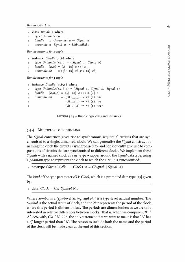
61

3.4.4śMultiple

clo

ckdomains

Bundle type class

1 class Bundle a where

2 type Unbundled a3 bundle :: Unbundled a → Signal a4 unbundle :: Signal a → Unbundled a

Bundle instance for 2-tuple

1 instance Bundle (a ,b) where

2 type Unbundled (a ,b) = ( Signal a , Signal b)3 bundle (a ,b) = (,) ⟨$⟩ a ⟨∗⟩ b4 unbundle ab = ( fst ⟨$⟩ ab ,snd ⟨$⟩ ab)

Bundle instance for 3-tuple

1 instance Bundle (a ,b , c) where

2 type Unbundled (a ,b , c) = ( Signal a , Signal b , Signal c)3 bundle (a ,b , c) = (,,) ⟨$⟩ a ⟨∗⟩ b ⟨∗⟩ c4 unbundle abc = ((λ(x ,_ ,_) → x) ⟨$⟩ abc5 ,( λ(_ ,x ,_) → x) ⟨$⟩ abc6 ,( λ(_ ,_ ,x) → x) ⟨$⟩ abc)

Listing 3.24 ś Bundle type class and instances

3.4.4 Multiple clock domains

he Signal constructs gives rise to synchronous sequential circuits that are syn-chronised to a single, unnamed, clock. We can generalise the Signal construct bynaming the clock the circuit is synchronised to, and consequently give rise to com-positions of circuits that are synchronised to diferent clocks. We implement theseSignals with a named clock as a newtypewrapper around the Signal data type, usinga phantom type to represent the clock to which the circuit is synchronised:

1 newtype CSignal ( clk :: Clock) a = CSignal ( Signal a)

he kind of the type parameter clk isClock, which is a promoted data type [75] givenby:

1 data Clock = Clk Symbol Nat

Where Symbol is a type-level String, and Nat is a type-level natural number. heSymbol is the actual name of clock, and the Nat represents the period of the clock,where this period is dimensionless. he periods are dimensionless as we are onlyinterested in relative diferences between clocks. hat is, when we compare, Clk "A" 725, with, Clk "B" 225, the only statement that we want to make is that "A" hasa 29

9longer period than "B". he reason to include both the name and the period

of the clock will be made clear at the end of this section.

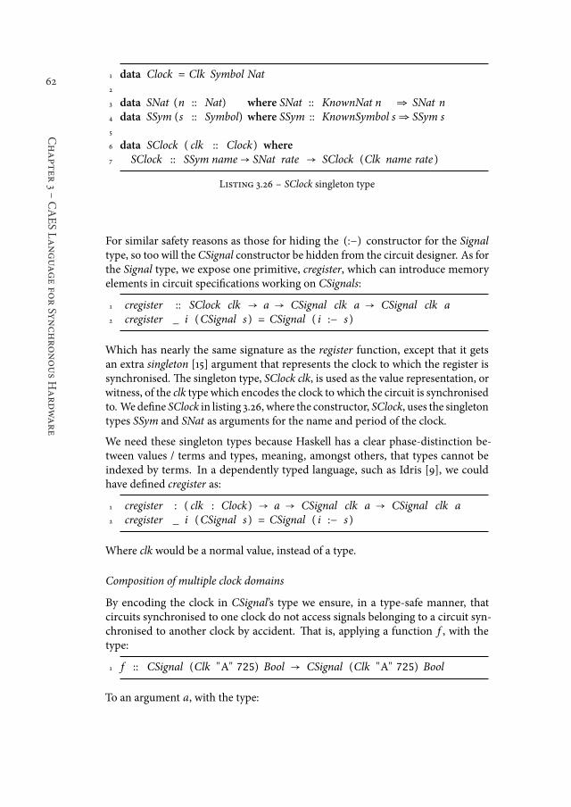
62

Chapter

3śCAESLanguagefo

rSynchronousHardware

1 data Clock = Clk Symbol Nat2

3 data SNat (n :: Nat) where SNat :: KnownNat n ⇒ SNat n4 data SSym (s :: Symbol) where SSym :: KnownSymbol s⇒ SSym s5

6 data SClock ( clk :: Clock) where7 SClock :: SSym name→ SNat rate → SClock (Clk name rate )

Listing 3.26 ś SClock singleton type

For similar safety reasons as those for hiding the (:−) constructor for the Signaltype, so too will the CSignal constructor be hidden from the circuit designer. As forthe Signal type, we expose one primitive, cregister, which can introduce memoryelements in circuit speciications working on CSignals:

1 cregister :: SClock clk → a → CSignal clk a → CSignal clk a2 cregister _ i (CSignal s ) = CSignal ( i :− s )

Which has nearly the same signature as the register function, except that it getsan extra singleton [15] argument that represents the clock to which the register issynchronised. he singleton type, SClock clk, is used as the value representation, orwitness, of the clk type which encodes the clock to which the circuit is synchronisedto. Wedeine SClock in listing 3.26, where the constructor, SClock, uses the singletontypes SSym and SNat as arguments for the name and period of the clock.

We need these singleton types because Haskell has a clear phase-distinction be-tween values / terms and types, meaning, amongst others, that types cannot beindexed by terms. In a dependently typed language, such as Idris [9], we couldhave deined cregister as:

1 cregister : ( clk : Clock) → a → CSignal clk a → CSignal clk a2 cregister _ i (CSignal s ) = CSignal ( i :− s )

Where clk would be a normal value, instead of a type.

Composition of multiple clock domains

By encoding the clock in CSignal’s type we ensure, in a type-safe manner, thatcircuits synchronised to one clock do not access signals belonging to a circuit syn-chronised to another clock by accident. hat is, applying a function f , with thetype:

1 f :: CSignal (Clk "A" 725) Bool → CSignal (Clk "A" 725) Bool

To an argument a, with the type:

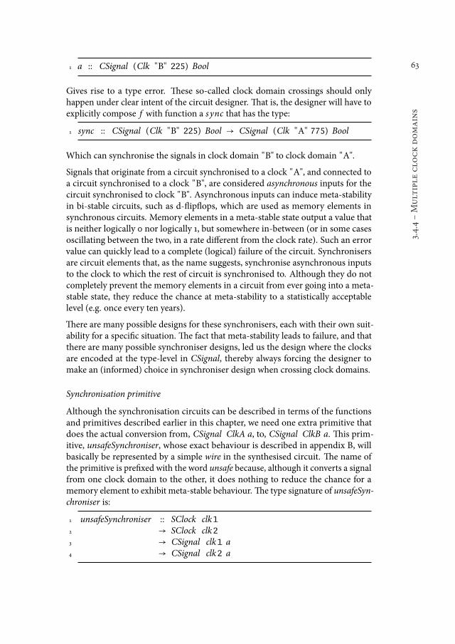
63

3.4.4śMultiple

clo

ckdomains

1 a :: CSignal (Clk "B" 225) Bool

Gives rise to a type error. hese so-called clock domain crossings should onlyhappen under clear intent of the circuit designer. hat is, the designer will have toexplicitly compose f with function a sync that has the type:

1 sync :: CSignal (Clk "B" 225) Bool → CSignal (Clk "A" 775) Bool

Which can synchronise the signals in clock domain "B" to clock domain "A".

Signals that originate from a circuit synchronised to a clock "A", and connected toa circuit synchronised to a clock "B", are considered asynchronous inputs for thecircuit synchronised to clock "B". Asynchronous inputs can induce meta-stabilityin bi-stable circuits, such as d-liplops, which are used as memory elements insynchronous circuits. Memory elements in a meta-stable state output a value thatis neither logically 0 nor logically 1, but somewhere in-between (or in some casesoscillating between the two, in a rate diferent from the clock rate). Such an errorvalue can quickly lead to a complete (logical) failure of the circuit. Synchronisersare circuit elements that, as the name suggests, synchronise asynchronous inputsto the clock to which the rest of circuit is synchronised to. Although they do notcompletely prevent the memory elements in a circuit from ever going into a meta-stable state, they reduce the chance at meta-stability to a statistically acceptablelevel (e.g. once every ten years).

here are many possible designs for these synchronisers, each with their own suit-ability for a speciic situation. he fact that meta-stability leads to failure, and thatthere are many possible synchroniser designs, led us the design where the clocksare encoded at the type-level in CSignal, thereby always forcing the designer tomake an (informed) choice in synchroniser design when crossing clock domains.

Synchronisation primitive

Although the synchronisation circuits can be described in terms of the functionsand primitives described earlier in this chapter, we need one extra primitive thatdoes the actual conversion from, CSignal ClkA a, to, CSignal ClkB a. his prim-itive, unsafeSynchroniser, whose exact behaviour is described in appendix B, willbasically be represented by a simple wire in the synthesised circuit. he name ofthe primitive is preixed with the word unsafe because, although it converts a signalfrom one clock domain to the other, it does nothing to reduce the chance for amemory element to exhibit meta-stable behaviour. he type signature of unsafeSyn-chroniser is:

1 unsafeSynchroniser :: SClock clk12 → SClock clk23 → CSignal clk1 a4 → CSignal clk2 a

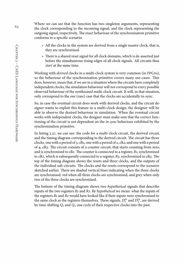
64

Chapter

3śCAESLanguagefo

rSynchronousHardware

Where we can see that the function has two singleton arguments, representingthe clock corresponding to the incoming signal, and the clock representing theoutgoing signal, respectively. he exact behaviour of the synchronisation primitiveconforms to a speciic scenario:

ż All the clocks in the system are derived from a single master clock, that is,they are synchronised.

ż here is a shared reset signal for all clock domains, which is de-asserted justbefore the simultaneous rising edges of all clock signals. All circuits thusstart at the same time.

Working with derived clocks in a multi-clock system is very common (in FPGAs),so the behaviour of the synchronisation primitive covers many use-cases. hisdoes, however, mean that, if we are in a situation where the circuits have completelyindependent clocks, the simulation behaviour will not correspond to every possibleobserved behaviour of the synthesised multi-clock circuit. It will, in that situation,only correspond to the one (rare) case that the clocks are accidentally in-sync.

So, in case the eventual circuit does work with derived clocks, and the circuit de-signer wants to exploit this feature in a multi-clock design, the designer will beable to observe the desired behaviour in simulation. When the eventual circuitworks with independent clocks, the designer must make sure that the correct func-tioning of the circuit is not dependent on the in-sync behaviour exhibited by thesynchronisation primitive.

In listing 3.27, we can see: the code for a multi-clock circuit, the derived circuit,and the timing diagram corresponding to the derived circuit. he circuit has threeclocks: onewith a period of 3, clk1, onewith a period of 2, clk2, and onewith a periodof 4, clk3. he circuit consists of a counter circuit, that starts counting from zero,and is synchronised to clk1. he counter is connected to a register, R1, synchronisedto clk2, which is subsequently connected to a register, R2, synchronised to clk3. hetop of the timing diagram shows the resets and three clocks, and the outputs ofthe individual sub-circuits. he clocks and the resets correspond to the scenariosketched earlier. here are shaded vertical lines indicating when the three clocksare synchronised: red when all three clocks are synchronised, and grey when onlytwo of the three clocks are synchronised.

he bottom of the timing diagram shows two hypothetical signals that describeinputs of the two registers R1 and R2. By hypothetical we mean: what the inputs ofthe registers R1 and R2 would have looked like if their inputs were synchronised tothe same clock as the registers themselves. hese signals, Din

1 and Din2 , are derived

by time-shiting Q1 and Q2 one cycle of their respective clocks into the past.

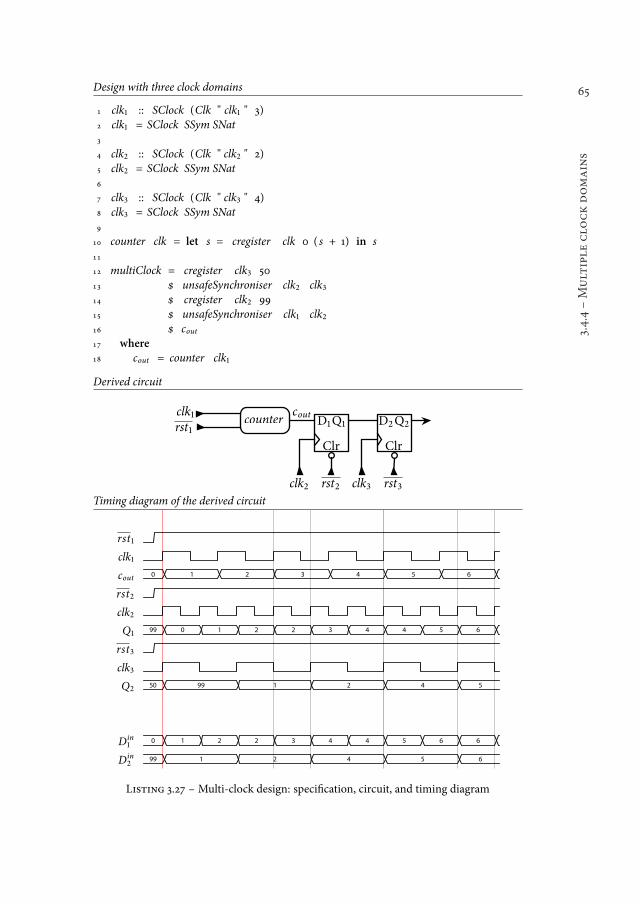
65

3.4.4śMultiple

clo

ckdomains

Design with three clock domains

1 clk1 :: SClock (Clk " clk1 " 3)2 clk1 = SClock SSym SNat3

4 clk2 :: SClock (Clk " clk2 " 2)5 clk2 = SClock SSym SNat6

7 clk3 :: SClock (Clk " clk3 " 4)8 clk3 = SClock SSym SNat9

10 counter clk = let s = cregister clk 0 ( s + 1) in s11

12 multiClock = cregister clk3 5013 $ unsafeSynchroniser clk2 clk314 $ cregister clk2 9915 $ unsafeSynchroniser clk1 clk216 $ cout17 where

18 cout = counter clk1

Derived circuit

rst�

clk� counter

Clr Clr

D� D�Q�Q�

clk� clk�

cout

rst� rst�Timing diagram of the derived circuit

rst1

clk1

cout 0 1 2 3 4 5 6

rst2

clk2

Q1 99 0 1 2 2 3 4 4 5 6

rst3

clk3

Q2 50 99 1 2 4 5

Din1

0 1 2 2 3 4 4 5 6 6

Din2

99 1 2 4 5 6

Listing 3.27 ś Multi-clock design: speciication, circuit, and timing diagram

66

Chapter

3śCAESLanguagefo

rSynchronousHardware

he synchronisation primitive, unsafeSynchroniser, is responsible for the creationof the streams corresponding to the timing diagrams of these hypothetical signals.So:

ż Given the stream of values corresponding to the timing diagram of cout :[0 ,1 ,2 ,3 ,4 , ..) .

ż he unsafeSynchroniser primitive creates the oversampled signal that corre-sponds to the timing diagram of Din

1 : [0 ,1 ,2 ,2 ,3 ,4 ,4 , ..) .

Similarly:

ż Given the stream of values corresponding to the timing diagram of Q1: [99,0 ,1 ,2 ,2 ,3 ,4 ,4 , ..) .

ż he unsafeSynchroniser primitive creates the compressed signal correspond-ing to the timing diagram of Din

2 : [99,1 ,2 ,4 , ..) .

Final remarks

Earlier we said we would explain why both the name and period of the clock areencoded in the Clk type: the reason that we do is to have a simple and safe synchro-nisation primitive. We encode the name of the clock so that we can distinguishtwo independent clocks that have the same period. Two independent clocks, evenif they have the same period, must always be synchronised for the meta-stabilityreasons stated earlier. We should hence not model such a system as having a singleclock. Choosing to encode the characteristics that set independent clocks withthe same period apart, such as phase-diference and drit-rates, would complicateboth the CSignal type, and the behaviour of the unsafeSynchroniser primitive. Onlyencoding the name, but not the period, of the clock is potentially unsafe: it wouldlead to a design where the periods would be speciied as part of unsafeSynchroniser.his could give rise to situations where the same clock is erroneously attributedwith diferent periods at distinct locations of unsafeSynchroniser.

3.5 Conclusions and future work

his chapter showed how we can model / specify both combinational and syn-chronous sequential circuits in CλaSH. Under the structural view, we can reasonstraightforwardly how a speciication is synthesised to a circuit. In general, ev-ery function application is synthesised to an instantiation of the correspondingcomponent. As a result, synthesised circuits are maximally parallel given their spec-iication. A downside of the structural view is that sequential execution has to bemanually speciied: a designer will need to specify his own control logic to executean algorithm sequentially. In SAFL [47] for example, which takes a behaviouralsynthesis approach, functions are only instantiated once, and function applicationis translated to control logic to facilitate concurrent access resulting from multiple

67

3.5śConclu

sionsandfu

turework

function applications. In SAFL we would thus get a circuit that is (almost5) maxi-mally sequential, and we have to duplicate functions to get a more parallel circuit.In Verity [22] there is also no need to specify one’s own control logic: recursionusing its ix-point construct is mapped to sequential circuitry. Parallel composition,however, has to be manually speciied.

In CλaSH, we model feedback loops by value recursion. Haskell’s non-strict eval-uation mechanism makes both the speciication and simulation of these circuitspeciications far more natural than in a strict setting. In a strict setting, in orderto simulate our speciications, we would have to make sure that all computationsinvolved in a feedback loop are properly delayed by creating a thunk. One strictoperation somewhere in the function hierarchy would force the complete computa-tion of the feedback loop. Aswe cannot know if a functionwill be used in a feedbackloop, we can only anticipate by creating thunks everywhere, basically mimickingnon-strict evaluation.

In an earlier version of CλaSH, [CB:7], we did not use the Signal type to modelthe values manipulated by synchronous sequential circuits. Instead, we modelledsynchronous sequential circuits by solely describing the combinational part of aMealy machine (in the same way as we have seen them in section 3.4.3). As a result,a composition of sequential circuits also had to be modelled in the form of a Mealymachine. Additionally, the arguments and result representing the state of the sub-components must be aggregated in the argument and result of the bigger Mealymachine. hat is, given two Mealy machine descriptions, f and g, the function hthat composes them will look, in general form, like:

1 h (( fS ,gS) ,hS) inp = ((( fS ’, gS ’) ,hS ’) ,outp)2 where3 ( fS ’, ...) = f fS ...4 (gS ’, ...) = g gS ...5 hS ’ = ...6 outp = ...

Where fS, gS, fS’, and gS’, correspond to the state of f and g, and, hS and hS’ corre-spond to the state of h. he downside of this old approach is that the aggregationis very repetitive, pollutes the local namespace of a function, and is prone to errorsthat break the Mealy machine abstraction. By the latter we mean that sub-states ofthe Mealy machines must be aggregated unchanged, and the current and updatedstates have to appear in the same order across the argument and the result. hat is,the following deinition of h would be erroneous:

1 h (( fS ,gS) ,hS) inp = ((( gS ’, fS ’) ,hS ’) ,outp)2 where3 ...

5Primitive operations in SAFL are implicitly duplicated, and will hence operate in parallel.

68

Chapter

3śCAESLanguagefo

rSynchronousHardware

Where the updated state of g, gS’, is aggregated as the updated state of f , and visa-versa. Depending on the types of fS’ and gS’, such a switch might be caught as atype-error, or it might, in a more unfortunate situation, not be caught as a typeerror.

In [CB:9] we describe how we encapsulate our Mealy machines description inan automata arrow [53], and use the arrow notation [52] for the composition ofsequential circuits. he encapsulation in an automata arrow abstracts the processof subdivision and aggregations of substates, thus solving the problems mentionedearlier regarding manual subdivision and aggregation. Using arrows does, however,have two downsides:

ż Arrows can only have one input: multiple inputs must hence be aggregatedin a tuple. Functions / Arrows representing a sequential circuit can hencenot be speciied in a curried form. Consequently, if one wants to partiallyapply an arrow, he / she will need to wrap the arrow in a lambda abstractionirst.

ż he arrow notation has its own local scope, meaning variables bound withinthe arrow notation can only be referenced within the arrow-notation block,and not from the where clause.

By using the Signal type as presented in this chapter we sufer from neither of theabove problems:

ż here is no special syntax for the composition of functions representingsequential circuits, and consequently no separate scope. Composition canbe done within regular where-clauses and let -expressions.

ż We are not forced to aggregate the inputs of a function representing a sequen-tial circuit into a tuple, meaning that a sequential circuit can be modelledas a curried function. Consequently, partial application of a function rep-resenting a sequential circuit is just as straightforward as partially applyingany other curried function.

3.5.1 Future work

Working with values of the Signal type precludes the use of straightforward patternmatching in the speciications of sequential circuits. In section 3.4.3 we already sawthat a Signal of a product type is isomorphic to the product of Signal types, a factexploited by the Bundle type-class. Pattern matching on Signals of product typesis hence possible by manually inserting unbundle at the place we want to patternmatch. A possible extension, beyond what is currently supported by either Haskellor the language extensions of GHC, is to insert bundle and unbundle automati-cally, knowing that the isomorphism in the Bundle type class is guaranteed by thesynchronisity assumption underlying Signal. We could subsequently use patternmatching on product types in speciications of sequential circuits, without havingto worry where to add bundle and unbundle.

69

3.5.1śFu

turework

Pattern matching on Signals of sum types is even more diicult. First of all, thereis no isomorphism between a Signal of a sum-type, and a sum(-of-products) of aSignal, meaning that we cannot deine a Bundle instance for sum types. What is,however, possible is to emulate patterns and pattern matching using the techniquesfor Lava, shown earlier in chapter 2. he disadvantages of those techniques havealso already been described in chapter 2. hose techniques also do not ofer a wayfor functions to be deined in terms of multiple clauses. Future work lies in dein-ing a synchronous semantics for pattern matching on sum-types from which animplementation, perhaps using source-to-source transformations to a speciicationusing the techniques in chapter 2, can follow.

70

71

4Type-Directed Synthesis

Abstract ś A straightforward synthesis from functional languages to digitalcircuits transforms variables towires. he types of these variables determine thebit-width of the wires. Assigning a bit-width to polymorphic and function-typevariables within this direct synthesis scheme is impossible. Using a term rewritesystem, polymorphic and function-type binders can be completely eliminatedfrom a circuit description, given only minor and reasonable restrictions on theinput.

4.1 Introduction

In the previous chapter we discussed the use of Haskell for speciications of syn-chronous digital circuits and the structural interpretation of these descriptions.his chapter will discuss the CλaSH compiler, whose purpose is to produce a netlistfrom the high-level Haskell description. Industry standard tools can then be usedfor further processing, such a programming an FPGA or creating an ASIC.

his chapter is split up roughly into two parts, the irst part describes the compilerpipeline and certain engineering details. he second part provides details aboutthe synthesis process. he translation from a (functional) description to a netlistis called synthesis in hardware literature (where it would be called compilation insotware literature). he set of rules and transformations that together describe theconversion procedure from description to netlist is called a synthesis scheme.

he CλaSH compiler uses a term rewrite system (TRS), with bound variables, todrive the synthesis process. he objective of the TRS is to produce a normal form ofthe description which can be trivially converted to a netlist. his chapter providesproofs that the transformations of the TRS preserve the types and semantics of

Parts of this chapter have been published in [CB:13]

72

Chapter

4śType-D

irec

ted

Synthesis

expressions. Additionally we prove that, given reasonable restrictions, the TRS willalways ind the normal form.

he next subsection gives both a deinition for netlists, and an introduction tosynthesis schemes by describing a speciic instance for a small functional language.he deinition and introduction are both informal, but hopefully instil an intuitionfor the process of transforming a functional description to an actual circuit.

4.1.1 Netlists & Synthesis

A netlist is a textual description of a digital circuit [17]. It lists the components thata circuit contains, and the connections between these components. he connectionpoints of a component are called ports, or pins. he ports are annotated with thebit-width of the values that low through them. A netlist can either be hierarchicalor lattened. In a hierarchical netlist, sub-netlists are abstracted to appear as singlecomponents, of which multiple instances can be created. By instantiating all ofthese instances, a lattened netlist can be created.

A synthesis scheme deines the procedure that transforms a (functional) descriptionto a netlist. Synthesis schemes deined for diferent languages, which nonethelesshave common aspects, will be called a synthesis scheme family. he CλaSH com-piler uses a synthesis scheme, which we will call TCλ , that is an instance of thelarger synthesis scheme family that will be referred to as T . he following aspectsare shared by all instances of T :

ż It is completely syntax-directed.

ż It creates a hierarchical netlist.

ż Function deinitions are translated to components, where the argumentsof the function become the input ports, and the result is connected to theoutput port.

ż Function application is translated to an instance of the component that rep-resents the corresponding function. he applied arguments are connectedto the input ports of the component instance.

To demonstrate T , a simple functional language, L, is introduced in igure 4.1. L isa pure, simply-typed, irst-order functional language. A program in L consists of aset of function deinitions, which always includes themain function. Expressionsin L can be: variable references, primitives, or function application. Figure 4.3shows a small example program deined in the presented functional language.

he synthesis scheme for L, called TL, is deined by two transformations: J Kp andJ Ke , in which J Kp is initially applied to themain function to create the hierarchicalnetlist. A graphical deinition of the J Kp and J Ke transformations is depicted inigure 4.2. Again, the purpose of this subsection is to give an intuition for thesynthesis process, not to give a formal account of TL. he transformation J Kpcreates a component deinition for a function f , where input ports correspond to

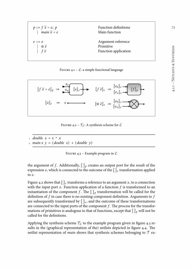
73

4.1.1śNetlists&Synthesis

p ::= f x ≙ e; p Function deinitions∣ main x ≙ e Main function

e ::= x Argument reference∣ ⊗ e Primitive∣ f e Function application

Figure 4.1 ś L: a simple functional language

J f x = eKp JeKe

x�

xn⇒

JxKe J⊗ eKe

J f eKe

⇒

⇒

⇒

Je�Ke

JenKe

xJe�KeJenKe

J f Kp

Figure 4.2 ś TL: A synthesis scheme for L

1 double x = x * x2 main x y = (double x) + (double y)

Figure 4.3 ś Example program in L

the argument of f . Additionally, J Kp creates an output port for the result of theexpression e, which is connected to the outcome of the J Ke transformation appliedto e.

Figure 4.2 shows that J Ke transforms a reference to an argument x, to a connectionwith the input port x. Function application of a function f is transformed to aninstantiation of the component f . he J Kp transformation will be called for thedeinition of f in case there is no existing component deinition. Arguments to fare subsequently transformed by J Ke , and the outcome of these transformationsare connected to the input ports of the component f . he process for the transfor-mations of primitives is analogous to that of functions, except that J Kp will not becalled for the deinitions.

Applying the synthesis scheme TL to the example program given in igure 4.3 re-sults in the (graphical representation of the) netlists depicted in igure 4.4. henetlist representation of main shows that synthesis schemes belonging to T ex-

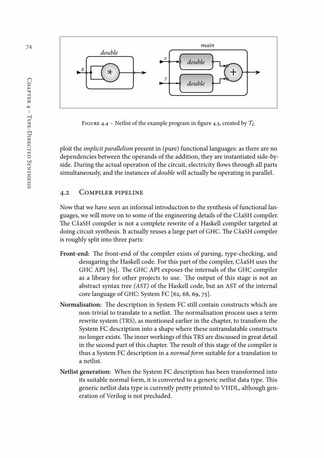
74

Chapter

4śType-D

irec

ted

Synthesis

double

y+

double

main

x

double

∗x

Figure 4.4 ś Netlist of the example program in igure 4.3, created by TL

ploit the implicit parallelism present in (pure) functional languages: as there are nodependencies between the operands of the addition, they are instantiated side-by-side. During the actual operation of the circuit, electricity lows through all partssimultaneously, and the instances of double will actually be operating in parallel.

4.2 Compiler pipeline

Now that we have seen an informal introduction to the synthesis of functional lan-guages, we will move on to some of the engineering details of the CλaSH compiler.he CλaSH compiler is not a complete rewrite of a Haskell compiler targeted atdoing circuit synthesis. It actually reuses a large part of GHC. he CλaSH compileris roughly split into three parts:

Front-end: he front-end of the compiler exists of parsing, type-checking, anddesugaring the Haskell code. For this part of the compiler, CλaSH uses theGHC API [65]. he GHC API exposes the internals of the GHC compileras a library for other projects to use. he output of this stage is not anabstract syntax tree (AST) of the Haskell code, but an AST of the internalcore language of GHC: System FC [62, 68, 69, 75].

Normalisation: he description in System FC still contain constructs which arenon-trivial to translate to a netlist. he normalisation process uses a termrewrite system (TRS), as mentioned earlier in the chapter, to transform theSystem FC description into a shape where these untranslatable constructsno longer exists. he inner workings of this TRS are discussed in great detailin the second part of this chapter. he result of this stage of the compiler isthus a System FC description in a normal form suitable for a translation toa netlist.

Netlist generation: When the System FC description has been transformed intoits suitable normal form, it is converted to a generic netlist data type. hisgeneric netlist data type is currently pretty printed to VHDL, although gen-eration of Verilog is not precluded.

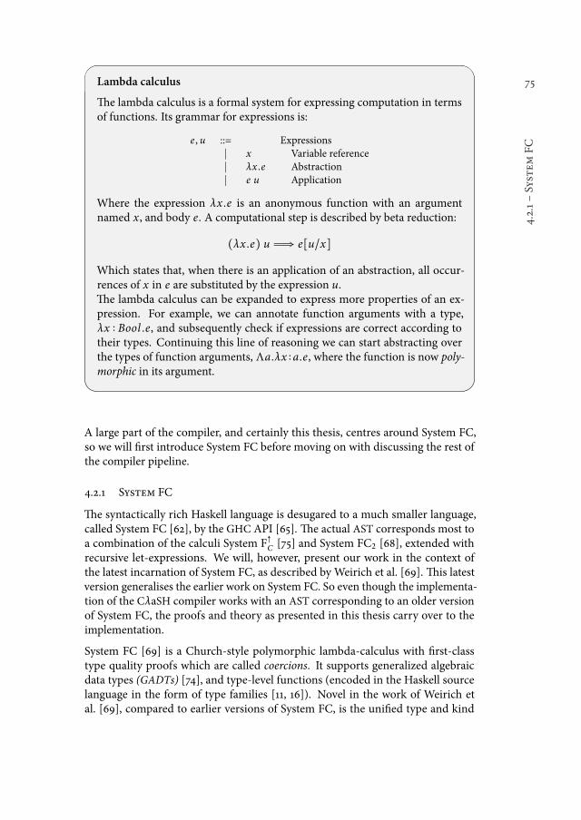
75

4.2.1śSystem

FC

Lambda calculus

he lambda calculus is a formal system for expressing computation in termsof functions. Its grammar for expressions is:

e , u ::= Expressions∣ x Variable reference∣ λx .e Abstraction∣ e u Application

Where the expression λx .e is an anonymous function with an argumentnamed x, and body e. A computational step is described by beta reduction:

(λx .e) uÔ⇒ e∥u/x∥

Which states that, when there is an application of an abstraction, all occur-rences of x in e are substituted by the expression u.he lambda calculus can be expanded to express more properties of an ex-pression. For example, we can annotate function arguments with a type,λx ∶ Bool .e, and subsequently check if expressions are correct according totheir types. Continuing this line of reasoning we can start abstracting overthe types of function arguments, Λa.λx ∶a.e, where the function is now poly-morphic in its argument.

A large part of the compiler, and certainly this thesis, centres around System FC,so we will irst introduce System FC before moving on with discussing the rest ofthe compiler pipeline.

4.2.1 System FC

he syntactically rich Haskell language is desugared to a much smaller language,called System FC [62], by the GHC API [65]. he actual AST corresponds most toa combination of the calculi System F↑C [75] and System FC2 [68], extended withrecursive let-expressions. We will, however, present our work in the context ofthe latest incarnation of System FC, as described by Weirich et al. [69]. his latestversion generalises the earlier work on System FC. So even though the implementa-tion of the CλaSH compiler works with an AST corresponding to an older versionof System FC, the proofs and theory as presented in this thesis carry over to theimplementation.

System FC [69] is a Church-style polymorphic lambda-calculus with irst-classtype quality proofs which are called coercions. It supports generalized algebraicdata types (GADTs) [74], and type-level functions (encoded in the Haskell sourcelanguage in the form of type families [11, 16]). Novel in the work of Weirich etal. [69], compared to earlier versions of System FC, is the uniied type and kind

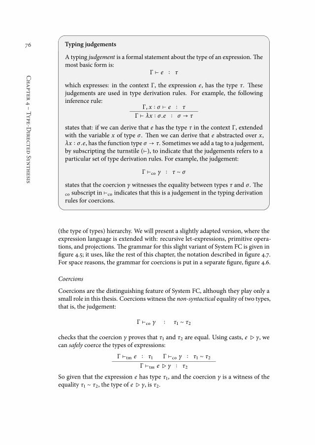
76

Chapter

4śType-D

irec

ted

Synthesis

Typing judgements

A typing judgement is a formal statement about the type of an expression. hemost basic form is:

Γ ⊢ e ∶ τ

which expresses: in the context Γ, the expression e, has the type τ. hesejudgements are used in type derivation rules. For example, the followinginference rule:

Γ, x ∶ σ ⊢ e ∶ τ

Γ ⊢ λx ∶ σ .e ∶ σ → τ

states that: if we can derive that e has the type τ in the context Γ, extendedwith the variable x of type σ . hen we can derive that e abstracted over x,λx ∶ σ .e, has the function type σ → τ. Sometimes we add a tag to a judgement,by subscripting the turnstile (⊢), to indicate that the judgements refers to aparticular set of type derivation rules. For example, the judgement:

Γ ⊢co γ ∶ τ ∼ σ

states that the coercion γ witnesses the equality between types τ and σ . he

co subscript in ⊢co indicates that this is a judgement in the typing derivationrules for coercions.

(the type of types) hierarchy. We will present a slightly adapted version, where theexpression language is extended with: recursive let-expressions, primitive opera-tions, and projections. he grammar for this slight variant of System FC is given inigure 4.5; it uses, like the rest of this chapter, the notation described in igure 4.7.For space reasons, the grammar for coercions is put in a separate igure, igure 4.6.

Coercions

Coercions are the distinguishing feature of System FC, although they play only asmall role in this thesis. Coercions witness the non-syntactical equality of two types,that is, the judgement:

Γ ⊢co γ ∶ τ1 ∼ τ2

checks that the coercion γ proves that τ1 and τ2 are equal. Using casts, e ▷ γ, wecan safely coerce the types of expressions:

Γ ⊢tm e ∶ τ1 Γ ⊢co γ ∶ τ1 ∼ τ2

Γ ⊢tm e▷ γ ∶ τ2

So given that the expression e has type τ1, and the coercion γ is a witness of theequality τ1 ∼ τ2, the type of e▷ γ, is τ2.

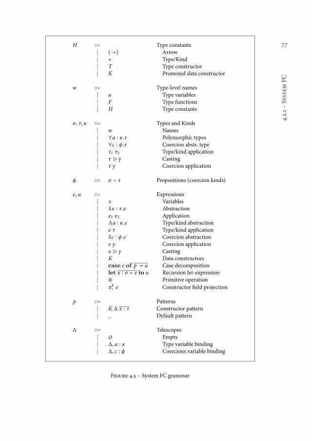
77

4.2.1śSystem

FC

H ∶∶≙ Type constants∣ (→) Arrow∣ ⋆ Type/Kind∣ T Type constructor∣ K Promoted data constructor

w ∶∶≙ Type-level names∣ a Type variables∣ F Type functions∣ H Type constants

σ , τ, κ ∶∶≙ Types and Kinds∣ w Names∣ ∀a ∶ κ.τ Polymorphic types∣ ∀c ∶ ϕ.τ Coercion abstr. type∣ τ1 τ2 Type/kind application∣ τ▷ γ Casting∣ τ γ Coercion application

ϕ ∶∶≙ σ ∼ τ Propositions (coercion kinds)

e , u ∶∶≙ Expressions∣ x Variables∣ λx ∶ τ.e Abstraction∣ e1 e2 Application∣ Λa ∶ κ.e Type/kind abstraction∣ e τ Type/kind application∣ λc ∶ ϕ.e Coercion abstraction∣ e γ Coercion application∣ e▷ γ Casting∣ K Data constructors∣ case e of p → u Case decomposition∣ let x ∶ σ ≙ e in u Recursion let-expression∣ ⊗ Primitive operation∣ πk

i e Constructor ield projection

p ∶∶≙ Patterns∣ K ∆ x ∶ τ Constructor pattern∣ _ Default pattern

∆ ∶∶≙ Telescopes∣ ∅ Empty∣ ∆, a ∶ κ Type variable binding∣ ∆, c ∶ ϕ Coercions variable binding

Figure 4.5 ś System FC grammar

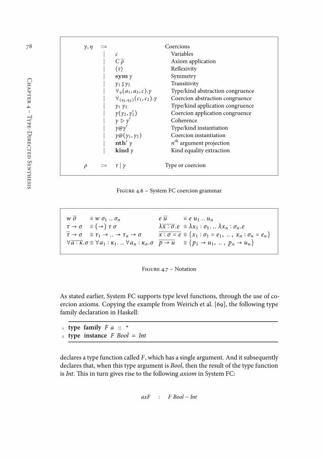
78

Chapter

4śType-D

irec

ted

Synthesis

γ, η ∶∶≙ Coercions∣ c Variables∣ C ρ Axiom application∣ ⟨τ⟩ Relexivity∣ sym γ Symmetry∣ γ1 o

9 γ2 Transitivity∣ ∀η(a1 , a2 , c).γ Type/kind abstraction congruence∣ ∀(η1 ,η2)(c1 , c2).γ Coercion abstraction congruence∣ γ1 γ2 Type/kind application congruence∣ γ(γ2 , γ

′2) Coercion application congruence

∣ γ▷ γ′ Coherence∣ γ@γ′ Type/kind instantiation∣ γ@(γ1 , γ2) Coercion instantiation∣ nthi γ nth argument projection∣ kind γ Kind equality extraction

ρ ∶∶≙ τ ∣ γ Type or coercion

Figure 4.6 ś System FC coercion grammar

w σ ≡ w σ1 .. σn e u ≡ e u1 .. un

τ → σ ≡ (→) τ σ λx ∶ σ .e ≡ λx1 ∶ σ1 . .. λxn ∶ σn .eτ → σ ≡ τ1 → .. → τn → σ x ∶ σ ≙ e ≡ {x1 ∶ σ1 ≙ e1 , .. , xn ∶ σn ≙ en}∀a ∶ κ.σ ≡ ∀a1 ∶ κ1 . .. ∀an ∶ κn .σ p → u ≡ {p1 → u1 , .. , pn → un}

Figure 4.7 ś Notation

As stated earlier, System FC supports type level functions, through the use of co-ercion axioms. Copying the example from Weirich et al. [69], the following typefamily declaration in Haskell:

1 type family F a :: *2 type instance F Bool = Int

declares a type function called F, which has a single argument. And it subsequentlydeclares that, when this type argument is Bool, then the result of the type functionis Int. his in turn gives rise to the following axiom in System FC:

axF : F Bool ∼ Int

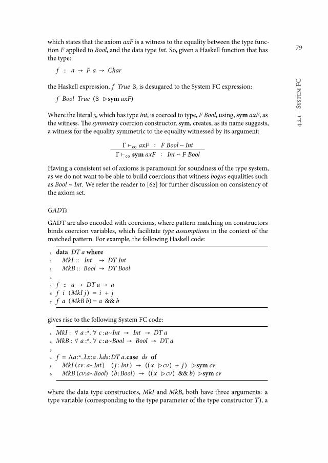
79

4.2.1śSystem

FC

which states that the axiom axF is a witness to the equality between the type func-tion F applied to Bool, and the data type Int. So, given a Haskell function that hasthe type:

f :: a → F a → Char

the Haskell expression, f True 3, is desugared to the System FC expression:

f Bool True (3 ▷sym axF)

Where the literal 3, which has type Int, is coerced to type, F Bool, using, sym axF, asthe witness. he symmetry coercion constructor, sym, creates, as its name suggests,a witness for the equality symmetric to the equality witnessed by its argument:

Γ ⊢co axF ∶ F Bool ∼ Int

Γ ⊢co sym axF ∶ Int ∼ F Bool

Having a consistent set of axioms is paramount for soundness of the type system,as we do not want to be able to build coercions that witness bogus equalities suchas Bool ∼ Int. We refer the reader to [62] for further discussion on consistency ofthe axiom set.

GADTs

GADT are also encoded with coercions, where pattern matching on constructorsbinds coercion variables, which facilitate type assumptions in the context of thematched pattern. For example, the following Haskell code:

1 data DT a where2 MkI :: Int → DT Int3 MkB :: Bool → DT Bool4

5 f :: a → DT a → a6 f i (MkI j) = i + j7 f a (MkB b) = a && b

gives rise to the following System FC code:

1 MkI : ∀ a :*. ∀ c :a~Int → Int → DT a2 MkB : ∀ a :*. ∀ c :a~Bool → Bool → DT a3

4 f = Λa :*.λx:a .λds :DT a.case ds of5 MkI (cv :a~Int) ( j : Int ) → ((x ▷cv) + j ) ▷sym cv6 MkB (cv:a~Bool) (b :Bool) → ((x ▷cv) && b)▷sym cv

where the data type constructors, MkI and MkB, both have three arguments: atype variable (corresponding to the type parameter of the type constructor T), a

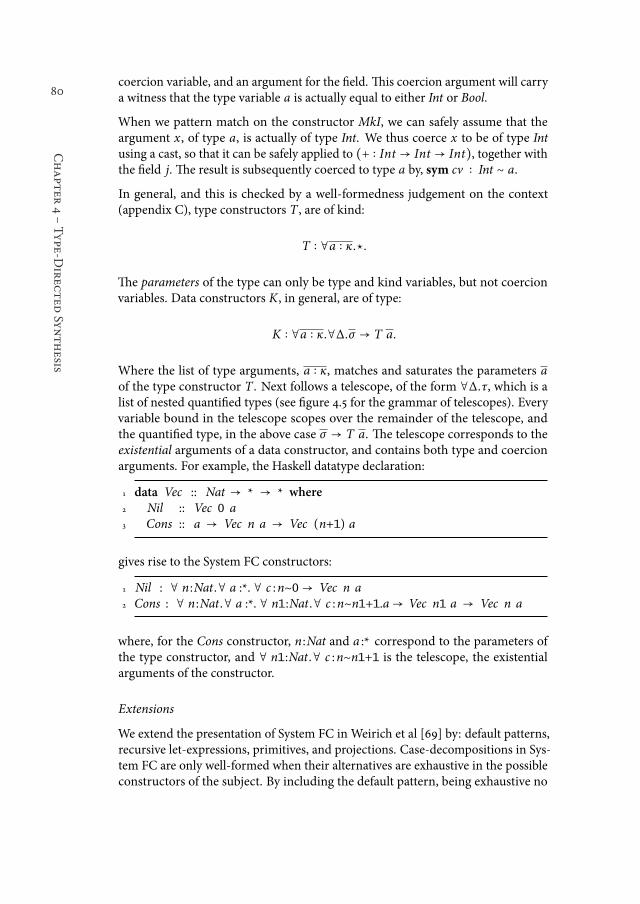
80

Chapter

4śType-D

irec

ted

Synthesis

coercion variable, and an argument for the ield. his coercion argument will carrya witness that the type variable a is actually equal to either Int or Bool.

When we pattern match on the constructor MkI, we can safely assume that theargument x, of type a, is actually of type Int. We thus coerce x to be of type Intusing a cast, so that it can be safely applied to (+ ∶ Int → Int → Int), together withthe ield j. he result is subsequently coerced to type a by, sym cv ∶ Int ∼ a.

In general, and this is checked by a well-formedness judgement on the context(appendix C), type constructors T , are of kind:

T ∶ ∀a ∶ κ.⋆.

he parameters of the type can only be type and kind variables, but not coercionvariables. Data constructors K, in general, are of type:

K ∶ ∀a ∶ κ.∀∆.σ → T a.

Where the list of type arguments, a ∶ κ, matches and saturates the parameters aof the type constructor T . Next follows a telescope, of the form ∀∆.τ, which is alist of nested quantiied types (see igure 4.5 for the grammar of telescopes). Everyvariable bound in the telescope scopes over the remainder of the telescope, andthe quantiied type, in the above case σ → T a. he telescope corresponds to theexistential arguments of a data constructor, and contains both type and coercionarguments. For example, the Haskell datatype declaration:

1 data Vec :: Nat → * → * where2 Nil :: Vec 0 a3 Cons :: a → Vec n a → Vec (n+1) a

gives rise to the System FC constructors:

1 Nil : ∀ n :Nat.∀ a :*. ∀ c :n~0→ Vec n a2 Cons : ∀ n :Nat.∀ a :*. ∀ n1:Nat.∀ c :n~n1+1.a→ Vec n1 a → Vec n a

where, for the Cons constructor, n :Nat and a :* correspond to the parameters ofthe type constructor, and ∀ n1:Nat.∀ c :n~n1+1 is the telescope, the existentialarguments of the constructor.

Extensions

We extend the presentation of System FC in Weirich et al [69] by: default patterns,recursive let-expressions, primitives, and projections. Case-decompositions in Sys-tem FC are only well-formed when their alternatives are exhaustive in the possibleconstructors of the subject. By including the default pattern, being exhaustive no

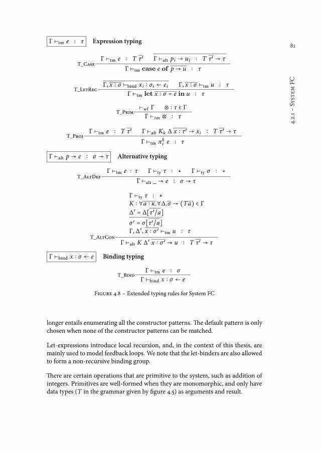
81

4.2.1śSystem

FC

Γ ⊢tm e ∶ τ Expression typing

T_CaseΓ ⊢tm e ∶ T τ′ Γ ⊢alt p i → u i ∶ T τ′ → τ

Γ ⊢tm case e of p → u ∶ τ

T_LetRecΓ, x ∶ σ ⊢bind x i ∶ σi ← e i Γ, x ∶ σ ⊢tm u ∶ τ

Γ ⊢tm let x ∶ σ ≙ e in u ∶ τ

T_Prim⊢wf Γ ⊗ ∶ τ ∈ Γ

Γ ⊢tm ⊗ ∶ τ

T_ProjΓ ⊢tm e ∶ T τ′ Γ ⊢alt Kk ∆ x ∶ τ′ → x i ∶ T τ′ → τ

Γ ⊢tm πki e ∶ τ

Γ ⊢alt p → e ∶ σ → τ Alternative typing

T_AltDefΓ ⊢tm e ∶ τ Γ ⊢ty τ ∶ ⋆ Γ ⊢ty σ ∶ ⋆

Γ ⊢alt _→ e ∶ σ → τ

T_AltCon

Γ ⊢ty τ ∶ ⋆K ∶ ∀a ∶ κ.∀∆.σ → (Ta) ∈ Γ

∆′ ≙ ∆∥τ′/a∥

σ ′ ≙ σ∥τ′/a∥Γ, ∆′ , x ∶ σ ′ ⊢tm u ∶ τ

Γ ⊢alt K ∆′ x ∶ σ ′ → u ∶ T τ′ → τ

Γ ⊢bind x ∶ σ ← e Binding typing

T_BindΓ ⊢tm e ∶ σ

Γ ⊢bind x ∶ σ ← e

Figure 4.8 ś Extended typing rules for System FC

longer entails enumerating all the constructor patterns. he default pattern is onlychosen when none of the constructor patterns can be matched.

Let-expressions introduce local recursion, and, in the context of this thesis, aremainly used to model feedback loops. We note that the let-binders are also allowedto form a non-recursive binding group.

here are certain operations that are primitive to the system, such as addition ofintegers. Primitives are well-formed when they are monomorphic, and only havedata types (T in the grammar given by igure 4.5) as arguments and result.

82

Chapter

4śType-D

irec

ted

Synthesis

he projection construct, πki e, projects (or extracts) the i’th ield of the k’th con-

structor of a data type T , from the expression e. his construct is not introduced bythe desugaring process fromHaskell to SystemFC. It is created by the normalisationprocess where it is (type-)safe to do. When the data type has only one constructorwe omit the k annotation, and just write π i .

We present the typing rules for these extensions in igure 4.8 and the operationalsemantics for the extensions in igures 4.9, 4.10, and 4.11. For an overview of all thetyping rules and operational semantics we refer the reader to appendix C. Most ofthe typing rules are straightforward.

In the typing rule for primitives, T_Prim, we perform a well-formedness check toensure that the primitive is monomorphic and only has data types (T) as argumentsand result. Type checking for alternatives has now moved to two separate judge-ments, of the form Γ ⊢alt p → e ∶ σ → τ, one for the default pattern (T_AltDef)and one for constructor patterns (T_AltCon). We refer the reader to [69] for theworkings of the typing judgement for constructor patterns. he type rule for projec-tion, T_Proj, uses the typing judgement for constructor pattern alternatives, wherethe matched constructor is the kth constructor of the data type, and the expressionis a variable reference to the ith ield of the constructor.

heT_LetRec rule is the typing-rule for recursive let-expressions. In the premise itsays that every binding i, x i ∶ σi ≙ e i , is checked in the context of the environment,Γ, and all let-bound variables, x ∶ σ , are checked using the bind typing rule ⊢bind.he typing rule for bindings says that, if the expression e has the type σ , then ebound to the variable x with type σ is a valid binding.

On to the operational semantics. To support recursion of let-expressions, we usean extra context Σlet that keeps track of the bindings in the recursive group. hisextra context does not inluence the proof of the type preservation theorem (theo-rem C.4.1) for the existing typing rules and operational semantics as presented in[69]. he rule S_LetRec, takes a step on the body of the let-expressions, with thebindings in scope of the extra context Σlet, and the result is the let-expression withthe one-step reduced body.

he progress theorem roughly states that if an expression is not a value, always oneof the step-reduction rules applies so that an evaluator for expressions can makeprogress. Values, and their types, value types, are deined by the grammar:

v ::= λx ∶ σ .e ∣ Λa ∶ κ.e ∣ λc ∶ ϕ.e ∣ K τ ρ e ∣ ⊗ vξ ::= σ1 → σ2 ∣ ∀a ∶ κ.σ ∣ ∀c ∶ ϕ.σ ∣ T σ

Compared to [69], we have extended our values with unsaturated primitives, ⊗ v.And, as we can see by the v, the arguments of a primitive are reduced to values,meaning that primitives are strict in all of their arguments. We also update thecanonical forms lemma, lemma 4.2.1.

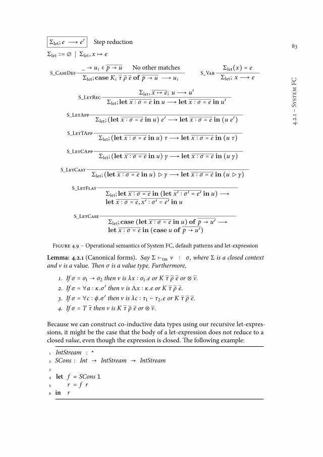
83

4.2.1śSystem

FC

Σlet; e Ð→ e′ Step reduction

Σlet ∶∶≙ ∅ ∣ Σlet , x ↦ e

S_CaseDef_→ u i ∈ p → u No other matches

Σlet;case K i τ ρ e of p → u Ð→ u i

S_VarΣlet(x) ≙ e

Σlet; x Ð→ e

S_LetRecΣlet , x ↦ e; u Ð→ u′

Σlet; let x ∶ σ ≙ e in u Ð→ let x ∶ σ ≙ e in u′

S_LetAppΣlet; (let x ∶ σ ≙ e in u) e′ Ð→ let x ∶ σ ≙ e in (u e′)

S_LetTAppΣlet; (let x ∶ σ ≙ e in u) τ Ð→ let x ∶ σ ≙ e in (u τ)

S_LetCAppΣlet; (let x ∶ σ ≙ e in u) γ Ð→ let x ∶ σ ≙ e in (u γ)

S_LetCastΣlet; (let x ∶ σ ≙ e in u)▷ γ Ð→ let x ∶ σ ≙ e in (u▷ γ)

S_LetFlat

Σlet; let x ∶ σ ≙ e in (let x′ ∶ σ ′ ≙ e′ in u)Ð→let x ∶ σ ≙ e , x′ ∶ σ ′ ≙ e′ in u

S_LetCase

Σlet;case (let x ∶ σ ≙ e in u) of p → u′ Ð→let x ∶ σ ≙ e in (case u of p → u′)

Figure 4.9 ś Operational semantics of System FC, default patterns and let-expression

Lemma: 4.2.1 (Canonical forms). Say Σ ⊢tm v ∶ σ , where Σ is a closed contextand v is a value. hen σ is a value type. Furthermore,

1. If σ ≙ σ1 → σ2 then v is λx ∶ σ1 .e or K τ ρ e or ⊗ v.

2. If σ ≙ ∀a ∶ κ.σ ′ then v is Λx ∶ κ.e or K τ ρ e.

3. If σ ≙ ∀c ∶ ϕ.σ ′ then v is λc ∶ τ1 ∼ τ2 .e or K τ ρ e.

4. If σ ≙ T τ then v is K τ ρ e or ⊗ v.

Because we can construct co-inductive data types using our recursive let-expres-sions, it might be the case that the body of a let-expression does not reduce to aclosed value, even though the expression is closed. he following example:

1 IntStream : *2 SCons : Int → IntStream → IntStream3

4 let f = SCons 15 r = f r6 in r

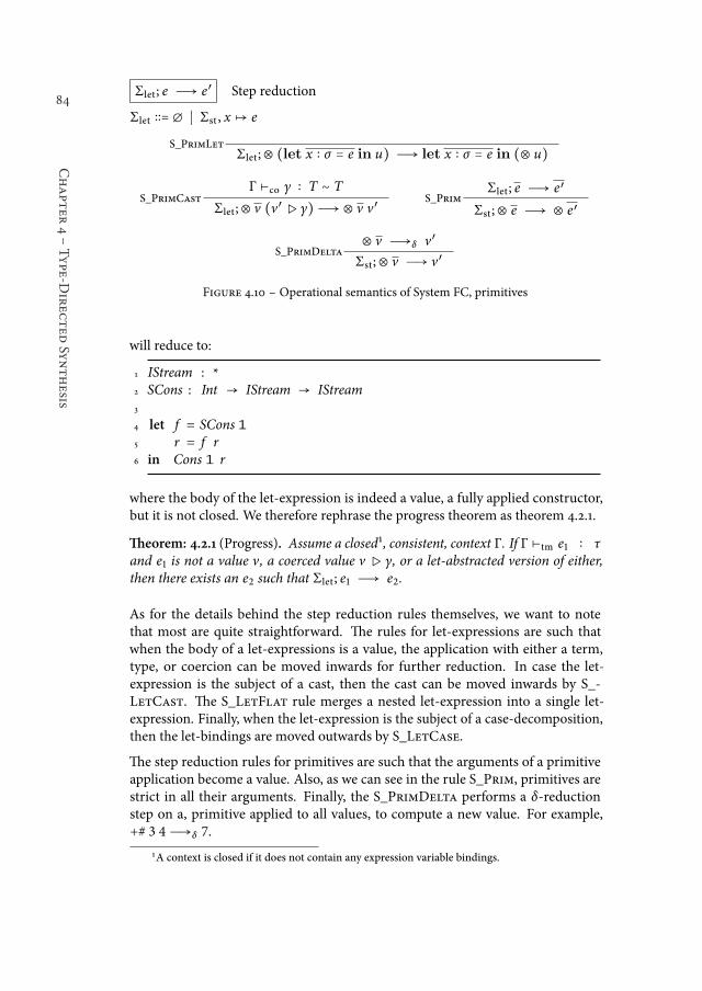
84

Chapter

4śType-D

irec

ted

Synthesis

Σlet; e Ð→ e′ Step reduction

Σlet ∶∶≙ ∅ ∣ Σst , x ↦ e

S_PrimLetΣlet;⊗ (let x ∶ σ ≙ e in u) Ð→ let x ∶ σ ≙ e in (⊗ u)

S_PrimCastΓ ⊢co γ ∶ T ∼ T

Σlet;⊗ v (v′▷ γ)Ð→ ⊗ v v′S_Prim

Σlet; e Ð→ e′

Σst;⊗ e Ð→ ⊗ e′

S_PrimDelta⊗ v Ð→δ v′

Σst;⊗ v Ð→ v′

Figure 4.10 ś Operational semantics of System FC, primitives

will reduce to:

1 IStream : *2 SCons : Int → IStream → IStream3

4 let f = SCons 15 r = f r6 in Cons 1 r

where the body of the let-expression is indeed a value, a fully applied constructor,but it is not closed. We therefore rephrase the progress theorem as theorem 4.2.1.

heorem: 4.2.1 (Progress). Assume a closed¹, consistent, context Γ. If Γ ⊢tm e1 ∶ τand e1 is not a value v, a coerced value v ▷ γ, or a let-abstracted version of either,then there exists an e2 such that Σlet; e1 Ð→ e2.

As for the details behind the step reduction rules themselves, we want to notethat most are quite straightforward. he rules for let-expressions are such thatwhen the body of a let-expressions is a value, the application with either a term,type, or coercion can be moved inwards for further reduction. In case the let-expression is the subject of a cast, then the cast can be moved inwards by S_-LetCast. he S_LetFlat rule merges a nested let-expression into a single let-expression. Finally, when the let-expression is the subject of a case-decomposition,then the let-bindings are moved outwards by S_LetCase.

he step reduction rules for primitives are such that the arguments of a primitiveapplication become a value. Also, as we can see in the rule S_Prim, primitives arestrict in all their arguments. Finally, the S_PrimDelta performs a δ-reductionstep on a, primitive applied to all values, to compute a new value. For example,+# 3 4Ð→δ 7.

1A context is closed if it does not contain any expression variable bindings.

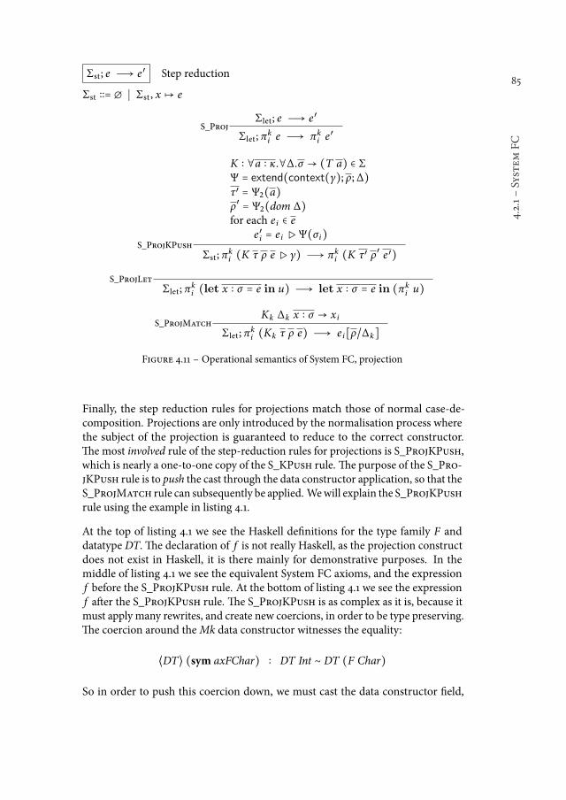
85

4.2.1śSystem

FC

Σst; e Ð→ e′ Step reduction

Σst ∶∶≙ ∅ ∣ Σst , x ↦ e

S_ProjΣlet; e Ð→ e′

Σlet; πki e Ð→ πk

i e′

S_ProjKPush

K ∶ ∀a ∶ κ.∀∆.σ → (T a) ∈ ΣΨ ≙ extend(context(γ); ρ;∆)τ′ ≙ Ψ2(a)ρ′ ≙ Ψ2(dom ∆)for each e i ∈ e

e′i ≙ e i ▷Ψ(σi)

Σst; πki (K τ ρ e▷ γ) Ð→ πk

i (K τ′ ρ′ e′)

S_ProjLet

Σlet; πki (let x ∶ σ ≙ e in u) Ð→ let x ∶ σ ≙ e in (πk

i u)

S_ProjMatchKk ∆k x ∶ σ → x i

Σlet; πki (Kk τ ρ e) Ð→ e i∥ρ/∆k∥

Figure 4.11 ś Operational semantics of System FC, projection

Finally, the step reduction rules for projections match those of normal case-de-composition. Projections are only introduced by the normalisation process wherethe subject of the projection is guaranteed to reduce to the correct constructor.he most involved rule of the step-reduction rules for projections is S_ProjKPush,which is nearly a one-to-one copy of the S_KPush rule. he purpose of the S_Pro-jKPush rule is to push the cast through the data constructor application, so that theS_ProjMatch rule can subsequently be applied. Wewill explain the S_ProjKPushrule using the example in listing 4.1.

At the top of listing 4.1 we see the Haskell deinitions for the type family F anddatatype DT. he declaration of f is not really Haskell, as the projection constructdoes not exist in Haskell, it is there mainly for demonstrative purposes. In themiddle of listing 4.1 we see the equivalent System FC axioms, and the expressionf before the S_ProjKPush rule. At the bottom of listing 4.1 we see the expressionf ater the S_ProjKPush rule. he S_ProjKPush is as complex as it is, because itmust apply many rewrites, and create new coercions, in order to be type preserving.he coercion around theMk data constructor witnesses the equality:

⟨DT⟩ (sym axFChar) ∶ DT Int ∼ DT (F Char)

So in order to push this coercion down, we must cast the data constructor ield,

86

Chapter

4śType-D

irec

ted

Synthesis

Haskell

1 type family F Int = Bool2 type family F Char = Int3

4 data DT a where5 Mk :: F a → DT a6

7 f :: F (F Char)8 f = π1 ((MkDT True :: DT Int) :: DT (F Char))

System FC, Before S_ProjPush

1 axFInt : F Int ~ Bool2 axFChar : F Char ~ Int3 Mk : ∀ a .F a → DT a4

5 f = π1 ((Mk Int (True ▷sym axFInt)) ▷(⟨DT⟩ (sym axFChar)))

System FC, Ater S_ProjPush

1 f = π1 (Mk (F Char) ((True ▷sym axFInt) ▷(⟨F⟩ nth1(⟨DT⟩ (sym axFChar)))))

Listing 4.1 ś S_ProjKPush Example

which before S_ProjKPush has type:

Γ ⊢tm True ∶ Bool Γ ⊢co sym axFInt ∶ Bool ∼ F Int

Γ ⊢tm True▷ sym axFInt ∶ F Int

to be of type, F (F Char), ater the application of S_ProjKPush. To do this, wecreate the coercion:

Γ ⊢co ⟨F⟩ ∶ F ∼ F Γ ⊢co nth1(⟨DT⟩ (sym axFChar)) ∶ Int ∼ F (Char)

Γ ⊢co ⟨F⟩ nth1(⟨DT⟩ (sym axFChar)) ∶ F Int ∼ F (F Char)

he operation that performs all transformations is called the liting operation, Ψ(⋅).he liting operation uses the liting context Ψ to know which rewrites it should per-form and how new coercions should be created. Elaboration of the liting context,the liting operation, and the functions: extend, and context, that are needed tobuild the liting context, fall outside the scope of this thesis. We refer the reader tosection 5 of [69] for a complete explanation of these concepts.

A complete overview of the typing rules and operational semantics can be found inappendix C, accompanied with the proofs for type preservation and progress. Wenow move on to discussing the remainder of the compiler pipeline.

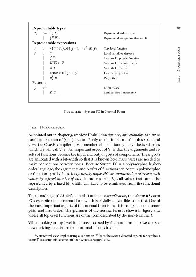
87

4.2.2śNormalfo

rm

Representable typesτr ::= Tr τr Representable data types

∣ (F τ)r Representable type function result

Representable expressions

t ::= λ(x ∶ τr).let y ∶ τr ≙ r+in y j Top-level function

r ::= x Local variable reference

∣ f x Saturated top-level function

∣ K τr ∅ x Saturated data constructor

∣ ⊗ x Saturated primitive

∣ case x of p → y Case decomposition

∣ πki x Projection

Patternsp ::= _ Default case

∣ K ∅ _ Matches data constructor

Figure 4.12 ś System FC in Normal Form

4.2.2 Normal form

As pointed out in chapter 3, we view Haskell descriptions, operationally, as a struc-tural composition of (sub-)circuits. Partly as a bi-implication² to this structuralview, the CλaSH compiler uses a member of the T family of synthesis schemes,which we will call TCλ . An important aspect of T is that the arguments and re-sults of functions become the input and output ports of components. hese portsare annotated with a bit-width so that it is known how many wires are needed tomake connections between ports. Because System FC is a polymorphic, higher-order language, the arguments and results of functions can contain polymorphicor function-typed values. It is generally impossible or impractical to represent suchvalues by a ixed number of bits. In order to run TCλ , all values that cannot berepresented by a ixed bit-width, will have to be eliminated from the functionaldescription.

he second stage ofCλaSH’s compilation chain, normalisation, transforms a SystemFC description into a normal form which is trivially convertible to a netlist. One ofthe most important aspects of this normal from is that it is completely monomor-phic, and irst-order. he grammar of the normal form is shown in igure 4.12,where all top-level functions are of the from described by the non-terminal t.

When looking at top-level functions accepted by the non-terminal t we can seehow deriving a netlist from our normal-form is trivial:

2A structural view implies using a variant on T (sans the syntax-directed aspect) for synthesis,using T as a synthesis scheme implies having a structural view.

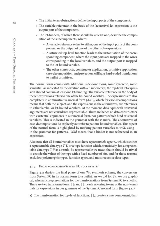
88

Chapter

4śType-D

irec

ted

Synthesis

ż he initial term-abstractions deine the input ports of the component.

ż he variable reference in the body of the (recursive) let-expression is theoutput port of the component.

ż he let-binders, of which there should be at least one, describe the compo-sition of the subcomponents, where:

ś A variable reference refers to either, one of the input ports of the com-ponent, or the output of one of the other sub-expressions.

ś A saturated top-level function leads to the instantiation of the corre-sponding component, where the input ports are mapped to the wirescorresponding to the local variables, and the output port is mappedto the let-bound variable.

ś he other constructs, constructor application, primitive application,case-decomposition, and projection, will have hard-coded translationsto netlist primitives.

he normal form comes with additional side-conditions, some syntactic, somesemantic. As indicated by the overline with a + superscript, the top-level let-expres-sion should contain at least one let-binding. he variable reference in the body ofthe let-expressions refers to one of the let-bound variables. he expressions are alsocompletely in administrative normal form (ANF), which for case-decompositionsmeans that both the subject, and the expressions in the alternatives, are referencesto either lamba- or let-bound variables. At the moment, data types with existentialarguments are not considered representable. here are hence no data constructorswith existential arguments in our normal form, nor patterns which bind existentialvariables. his is indicated in the grammar with the ∅ mark. he alternatives ofcase-decompositions do explicitly not refer to pattern-bound variables. his aspectof the normal form is highlighted by marking pattern variables as wild, using _,in the grammar for patterns. Wild means that a binder is not referenced in anexpression.

Also note that all bound variables must have representable type τt , which is eithera representable data type T τ, or a type function which, transitively, has a represen-table data type T τ as a result. By representable we mean that it should be trivialto encode the values of the type with a ixed number of bits, and for those reasonsexcludes: polymorphic types, function types, and most recursive data types.

4.2.3 From normalised System FC to a netlist

Figure 4.13 depicts the inal phase of our TCλ synthesis scheme, the conversionfrom System FC in its normal form to a netlist. As we did for TL, we use graphi-cal, schematic, representations for the transformations from System FC to a netlist.here are two transformations: J Kt and J Kr , each referring to one of the non-termi-nals for expressions in our grammar of the System FC normal form (igure 4.12).

a) he transformation for top-level functions, J Kt , creates a new component, that:

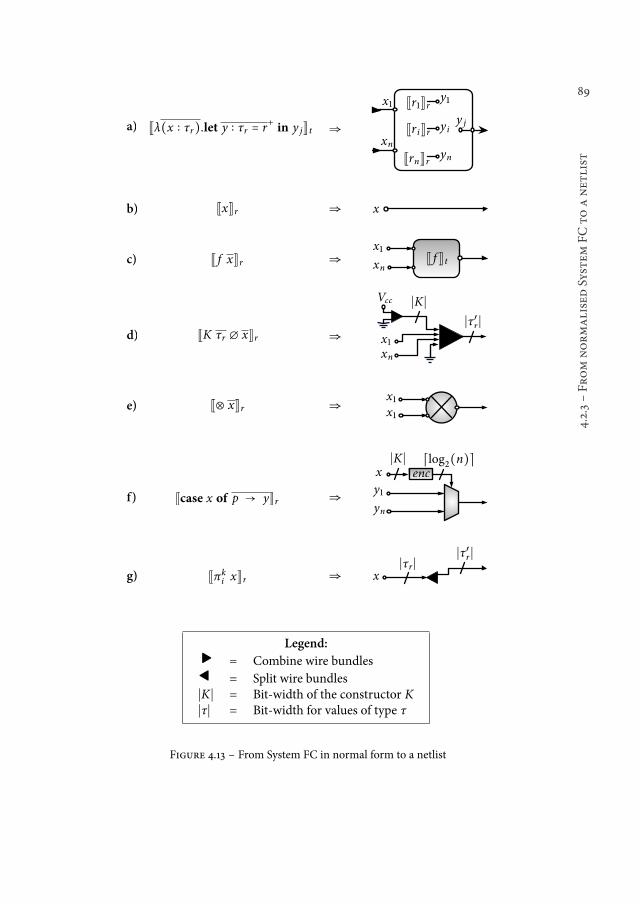
89

4.2.3śFr

omnormalisedSystem

FCto

anetlist

Jλ(x ∶ τr).let y ∶ τr = r+

in y jKt

Jr�Krx�

xn

⇒

JxKr

J⊗ xKr

J f xKr

⇒

⇒

⇒

x

J f Kt

Jr iKr

JrnKr

y�

y i

yn

y j

xn

JK τr � xKr ⇒

�K�

x�

Jcase x of p → yKr ⇒

y�

yn

Jπk

ixKr ⇒

�τr ��τ′r �

x

enc

�log�(n)��K�

x

xn

x�

�τ′r �

x�

x�

Vcc

a)

b)

c)

d)

e)

f)

g)

Legend:

� = Combine wire bundles

� = Split wire bundles�K� = Bit-width of the constructor K�τ� = Bit-width for values of type τ

Figure 4.13 ś From System FC in normal form to a netlist

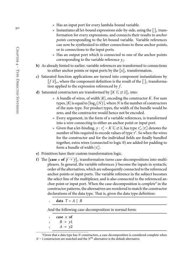
90

Chapter

4śType-D

irec

ted

Synthesis

ż Has an input port for every lambda-bound variable.ż Instantiates all let-bound expressions side-by-side, using the J Kr trans-formation for every expressions, and connects their results to anchorpoints corresponding to the let-bound variable. Variable referencescan now be synthesized to either connections to these anchor points,or to connections to the input ports.

ż Has an output port which is connected to one of the anchor pointscorresponding to the variable reference y j .

b) As already hinted to earlier, variable references are transformed to connectionsto either anchor points or input ports by the JxKr transformation.

c) Saturated function applications are turned into component instantiations byJ f xKr , where the component deinition is the result of the J Kt transforma-tion applied to the expression referenced by f .

d) Saturated constructors are transformed by JK τr ∅ xKr into:

ż A bundle of wires, of width ∣K∣, encoding the constructor K. For sumtypes, ∣K∣ is equal to ⌈log2(N)⌉, whereN is the number of constructorsof the sum-type. For product types, the width of the bundle would bezero, and the constructor would hence not be encoded.

ż Every argument, in the form of a variable references, is transformedinto a wire connecting to either an anchor point or input port.

ż Given that a let-binding, y ∶ τ′r ≙ K τr ∅ x, has type τ′r , ∣τ′r ∣ denotes the

number of bits required to encode values of type τ′. So when the wiresfor the constructor and for the individual ields are inally bundledtogether, extra wires (connected to logic 0) are added for padding toform a bundle of width ∣τ′r ∣.

e) Primitives have their custom transformation logic.

f) he Jcase x of p → yKr transformation turns case-decompositions into multi-plexers. In general, the variable references y become the inputs in syntacticorder of the alternatives, which are subsequently connected to the referencedanchor points or input ports. he variable reference in the subject becomesthe select line of the multiplexer, and is also connected to the referenced an-chor point or input port. When the case-decomposition is complete³ in theconstructor patterns, the alternatives are reordered tomatch the constructordeclarations of the data type. hat is, given the data type deinition:

1 data T = A | B

And the following case-decomposition in normal form:

1 case x of2 B → y13 A → y2

3Given that a data type has N constructors, a case-decomposition is considered complete whenN − 1 constructors are matched and the N th alternative is the default alternative.

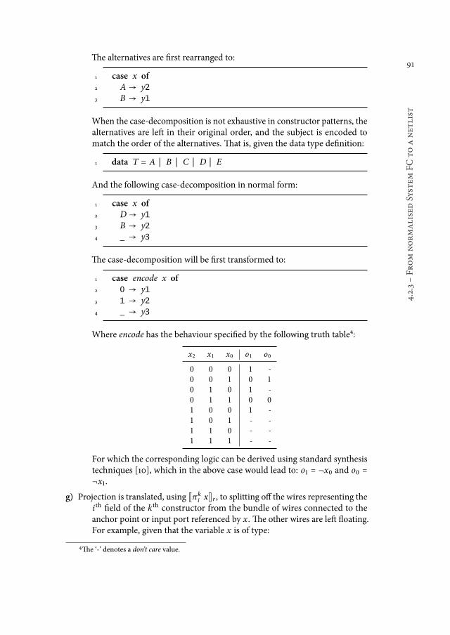
91

4.2.3śFr

omnormalisedSystem

FCto

anetlist

he alternatives are irst rearranged to:

1 case x of2 A → y23 B → y1

When the case-decomposition is not exhaustive in constructor patterns, thealternatives are let in their original order, and the subject is encoded tomatch the order of the alternatives. hat is, given the data type deinition:

1 data T = A | B | C | D | E

And the following case-decomposition in normal form:

1 case x of2 D→ y13 B → y24 _ → y3

he case-decomposition will be irst transformed to:

1 case encode x of2 0 → y13 1 → y24 _ → y3

Where encode has the behaviour speciied by the following truth table4:

x2 x1 x0 o1 o0

0 0 0 1 -

0 0 1 0 1

0 1 0 1 -

0 1 1 0 0

1 0 0 1 -

1 0 1 - -

1 1 0 - -

1 1 1 - -

For which the corresponding logic can be derived using standard synthesistechniques [10], which in the above case would lead to: o1 ≙ ¬x0 and o0 ≙¬x1.

g) Projection is translated, using Jπki xKr , to splitting of the wires representing the

ith ield of the kth constructor from the bundle of wires connected to theanchor point or input port referenced by x. he other wires are let loating.For example, given that the variable x is of type:

4he ‘-’ denotes a don’t care value.

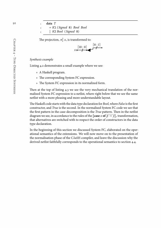
92

Chapter

4śType-D

irec

ted

Synthesis

1 data T2 = K1 (Signed 8) Bool Bool3 | K2 Bool (Signed 8)

he projection, π22 x, is transformed to:

[�� ∶ �][� ∶ �]

x

Synthesis example

Listing 4.2 demonstrates a small example where we see:

ż A Haskell program.

ż he corresponding System FC expression.

ż he System FC expression in its normalized form.

hen at the top of listing 4.3 we see the very mechanical translation of the nor-malised System FC expression to a netlist, where right below that we see the samenetlist with a more pleasing and more understandable layout.

heHaskell code startswith the data type declaration forBool, whereFalse is the irstconstructor, and True is the second. In the normalised System FC code we see thatthe irst pattern in the case-decomposition is the True pattern. hen in the netlistdiagramwe see, in accordance to the rules of the Jcase x of p → yKr transformation,that alternatives are switched with to respect the order of constructors in the datatype declaration.

In the beginning of this section we discussed System FC, elaborated on the oper-ational semantics of the extensions. We will now move on to the presentation ofthe normalisation phase of the CλaSH compiler, and leave the discussion why thederived netlist faithfully corresponds to the operational semantics to section 4.4.

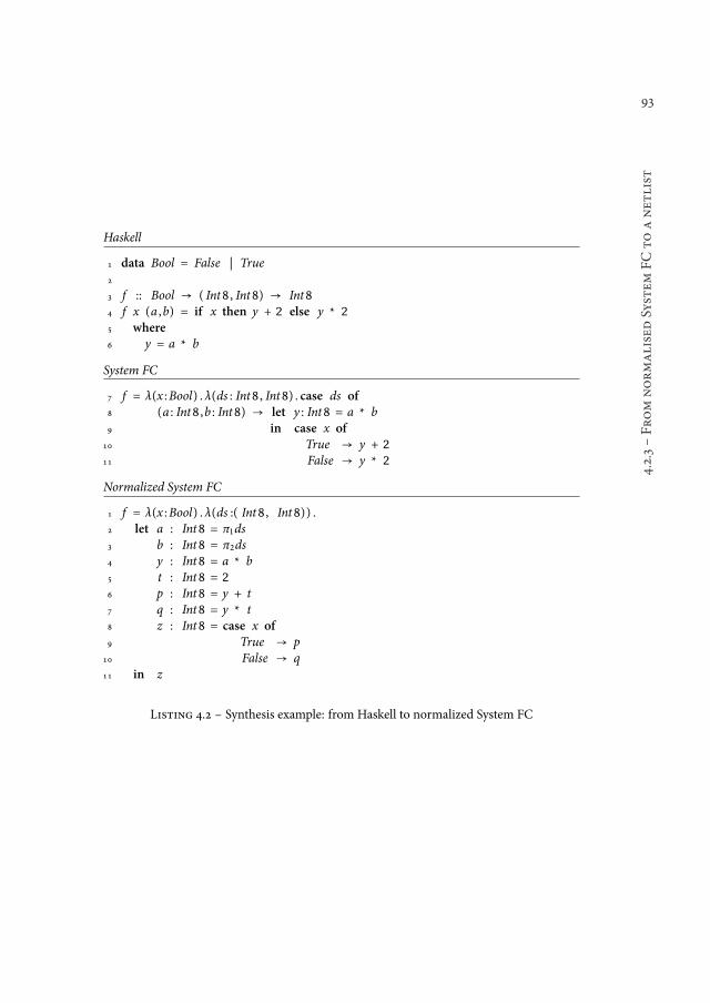
93

4.2.3śFr

omnormalisedSystem

FCto

anetlist

Haskell

1 data Bool = False | True2

3 f :: Bool → ( Int8 , Int8) → Int84 f x (a ,b) = if x then y + 2 else y * 2

5 where

6 y = a * b

System FC

7 f = λ(x :Bool) . λ(ds : Int8 , Int8) . case ds of

8 (a : Int8 ,b : Int8) → let y : Int8 = a * b9 in case x of

10 True → y + 2

11 False → y * 2

Normalized System FC

1 f = λ(x :Bool) . λ(ds :( Int8 , Int8)) .2 let a : Int8 = π1ds3 b : Int8 = π2ds4 y : Int8 = a * b5 t : Int8 = 2

6 p : Int8 = y + t7 q : Int8 = y * t8 z : Int8 = case x of

9 True → p10 False → q11 in z

Listing 4.2 ś Synthesis example: from Haskell to normalized System FC

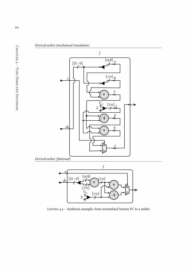
94

Chapter

4śType-D

irec

ted

Synthesis

Derived netlist (mechanical translation)

+

∗

a

bx

y

z

[��:�]

[�:�]

ds

p

q

f

�

�

∗

2t

[�:�]Vcc

[�� ∶ �]

Derived netlist (lattened)

+

∗

x

[��:�]

[�:�]

ds

f

�

�

∗

2

[�:�]Vcc

[�� ∶ �] [�:�]

Listing 4.3 ś Synthesis example: from normalized System FC to a netlist

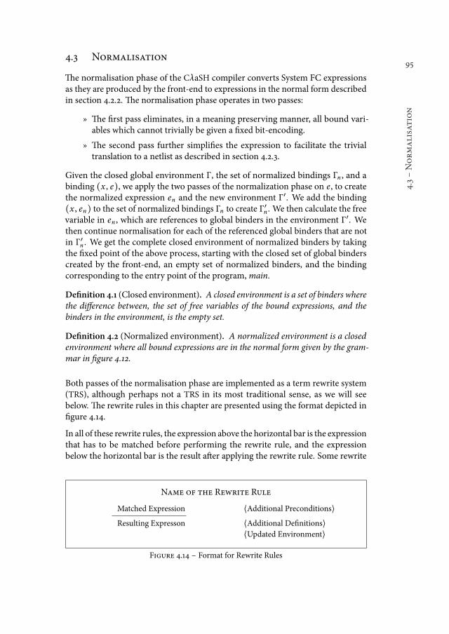
95

4.3śNormalisation

4.3 Normalisation

he normalisation phase of the CλaSH compiler converts System FC expressionsas they are produced by the front-end to expressions in the normal form describedin section 4.2.2. he normalisation phase operates in two passes:

ż he irst pass eliminates, in a meaning preserving manner, all bound vari-ables which cannot trivially be given a ixed bit-encoding.

ż he second pass further simpliies the expression to facilitate the trivialtranslation to a netlist as described in section 4.2.3.

Given the closed global environment Γ, the set of normalized bindings Γn , and abinding (x , e), we apply the two passes of the normalization phase on e, to createthe normalized expression en and the new environment Γ′. We add the binding(x , en) to the set of normalized bindings Γn to create Γ′n . We then calculate the freevariable in en , which are references to global binders in the environment Γ′. Wethen continue normalisation for each of the referenced global binders that are notin Γ′n . We get the complete closed environment of normalized binders by takingthe ixed point of the above process, starting with the closed set of global binderscreated by the front-end, an empty set of normalized binders, and the bindingcorresponding to the entry point of the program,main.

Deinition 4.1 (Closed environment). A closed environment is a set of binders wherethe diference between, the set of free variables of the bound expressions, and thebinders in the environment, is the empty set.

Deinition 4.2 (Normalized environment). A normalized environment is a closedenvironment where all bound expressions are in the normal form given by the gram-mar in igure 4.12.

Both passes of the normalisation phase are implemented as a term rewrite system(TRS), although perhaps not a TRS in its most traditional sense, as we will seebelow. he rewrite rules in this chapter are presented using the format depicted inigure 4.14.

In all of these rewrite rules, the expression above the horizontal bar is the expressionthat has to be matched before performing the rewrite rule, and the expressionbelow the horizontal bar is the result ater applying the rewrite rule. Some rewrite

Name of the Rewrite Rule

Matched Expression ⟨Additional Preconditions⟩

Resulting Expresson ⟨Additional Deinitions⟩⟨Updated Environment⟩

Figure 4.14 ś Format for Rewrite Rules

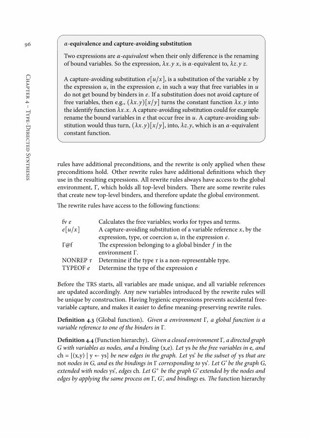
96

Chapter

4śType-D

irec

ted

Synthesis

α-equivalence and capture-avoiding substitution

Two expressions are α-equivalent when their only diference is the renamingof bound variables. So the expression, λx .y x, is α-equivalent to, λz.y z.

A capture-avoiding substitution e∥u/x∥, is a substitution of the variable x bythe expression u, in the expression e, in such a way that free variables in udo not get bound by binders in e. If a substitution does not avoid capture offree variables, then e.g., (λx .y)∥x/y∥ turns the constant function λx .y intothe identify function λx .x. A capture-avoiding substitution could for examplerename the bound variables in e that occur free in u. A capture-avoiding sub-stitution would thus turn, (λx .y)∥x/y∥, into, λz.y, which is an α-equivalentconstant function.

rules have additional preconditions, and the rewrite is only applied when thesepreconditions hold. Other rewrite rules have additional deinitions which theyuse in the resulting expressions. All rewrite rules always have access to the globalenvironment, Γ, which holds all top-level binders. here are some rewrite rulesthat create new top-level binders, and therefore update the global environment.

he rewrite rules have access to the following functions:

fv e Calculates the free variables; works for types and terms.e∥u/x∥ A capture-avoiding substitution of a variable reference x, by the

expression, type, or coercion u, in the expression e.Γ@f he expression belonging to a global binder f in the

environment Γ.NONREP τ Determine if the type τ is a non-representable type.TYPEOF e Determine the type of the expression e

Before the TRS starts, all variables are made unique, and all variable referencesare updated accordingly. Any new variables introduced by the rewrite rules willbe unique by construction. Having hygienic expressions prevents accidental free-variable capture, and makes it easier to deine meaning-preserving rewrite rules.

Deinition 4.3 (Global function). Given a environment Γ, a global function is avariable reference to one of the binders in Γ.

Deinition 4.4 (Function hierarchy). Given a closed environment Γ, a directed graphG with variables as nodes, and a binding (x,e). Let ys be the free variables in e, andch = [(x,y) | y ← ys] be new edges in the graph. Let ys’ be the subset of ys that arenot nodes in G, and es the bindings in Γ corresponding to ys’. Let G’ be the graph G,extended with nodes ys’, edges ch. Let G+ be the graph G’ extended by the nodes andedges by applying the same process on Γ, G’, and bindings es. he function hierarchy

97

4.3.1śEliminat

ingnon-represen

table

valu

es

is the graph G∗ created by taking the ixed point of the above process starting with anempty graph and the binding corresponding to the entry point of the program,main.

Aside from needing the obvious property that the normalisation phase shouldpreserve the meaning of expressions, there are two additional properties that wewish our normalisation phase to respect as much as possible:

ż It should keep the original function hierarchy intact where possible, becausethe netlist hierarchy will follow the function hierarchy under TCλ . Leavingthe function hierarchy intact will make it easier to relate the non-functionalproperties of the netlist, such as area and propagation delay, back to theoriginal function. If desired, it is always possible to latten parts of thehierarchy later on, going in the other direction is non-trivial.

ż Sharing should be preserved where possible. As seen in listing 4.2, synthe-sized circuits can also share the result of a computation by connecting theoutput port of one component to input ports of multiple other components.Any loss in sharing, will most likely lead to a duplication of componentinstantiations, and under TCλ ultimately lead to a larger circuit.

4.3.1 Eliminating non-representable values

TCλ can only synthesize functional descriptions if function arguments, let-bind-ings, and pattern-bound variables can be given a ixed bit-encoding. here arestraightforward encodings for certain primitive data types, and certain algebraicdata types, as we have seen in chapter 3. Data types with a ixed bit-encoding arecalled representable. Deriving a ixed bit-encoding for the following types is eithernot desired, or not possible:

ż Function types.

ż (Higher-rank) polymorphic types.

ż Data types with existential arguments, and consequently, all GADTs.

ż Recursively deined data types.

ż Data types that are composed of types that are not representable.

his section shows that the TRS responsible for the irst pass of the normalisationpass, the removal of non-representable values. It eliminates such values completely,given that the input adheres to the following restrictions:

ż hemain function is monomorphic.

ż he arguments and the result of themain function are representable.

ż he arguments and the result of primitives are representable.

he TRS uses a combination of inlining and specialisation, where specialisationtakes on two forms:

98

Chapter

4śType-D

irec

ted

Synthesis

ż Specialisation of a function on one of its arguments.

ż Elimination of a case-decomposition based on a known constructor.

Simply inlining all functions with non-representable arguments and results, andinlining all non-representable let-bindings, is either undesired or not possible. In-lining destroys the original function hierarchy, which we are trying to preserve, andmight also lead to loss in sharing.

Defunctionalisation

Reynolds-style defunctionalisation [57] is a well-known method for generating anequivalent irst-order program from a higher-order program. Reynolds’ methodcreates data types for arguments with a function-type. Instead of applying a higher-order function to a value with a function-type, it is applied to a constructor for thenewly introduced data type. Application of the functional argument is replaced bythe application of a mini-interpreter. Given the following higher-order program:

1 uncurry f (a ,b) = f a b2 main x = (uncurry (+) x) + (uncurry () x)

Reynolds’ method creates the following behaviourally equivalent irst-order pro-gram:

1 data Function = Plus | Sub2 apply Plus a b = (+) a b3 apply Sub a b = () a b4

5 uncurry f (a ,b) = apply f a b6 main x = (uncurry Plus x) + (uncurry Min x)

Reynolds’ method works on all programs, removes all functional arguments, andpreserves sharing. Although commonly deined and studied in the setting of thesimply typed lambda calculus, there are also variants [6, 56] of Reynolds’ methodsthat are correct within a polymorphic type system. he disadvantage of Reynolds’method is the introduction of the mini-interpreter (which takes on the form of theapply function in the example).

he apply function will be transformed into netlist that contains an adder andsubtracter whose results will be multiplexed to the output. In the above example,the apply function will be instantiated twice, naively leading to a circuit with threeadders, two subtracters, and two multiplexers. Of course, we can specialize the twocalls to uncurry, and subsequently apply, on their irst argument to get a circuitthat has only two adders, one subtracter, and no multiplexers. We will thereforenot use (a variant of) Reynolds’ method in the CλaSH compiler, but instead opt tospecialise functions on their function-typed arguments immediately.

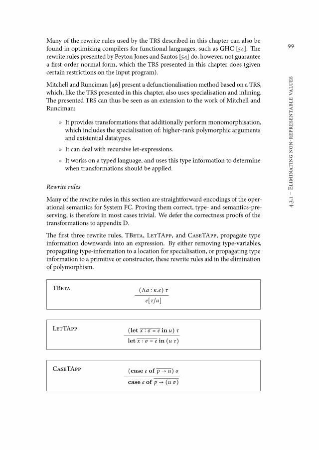
99

4.3.1śEliminat

ingnon-represen

table

valu

es

Many of the rewrite rules used by the TRS described in this chapter can also befound in optimizing compilers for functional languages, such as GHC [54]. herewrite rules presented by Peyton Jones and Santos [54] do, however, not guaranteea irst-order normal form, which the TRS presented in this chapter does (givencertain restrictions on the input program).

Mitchell and Runciman [46] present a defunctionalisation method based on a TRS,which, like the TRS presented in this chapter, also uses specialisation and inlining.he presented TRS can thus be seen as an extension to the work of Mitchell andRunciman:

ż It provides transformations that additionally perform monomorphisation,which includes the specialisation of: higher-rank polymorphic argumentsand existential datatypes.

ż It can deal with recursive let-expressions.

ż It works on a typed language, and uses this type information to determinewhen transformations should be applied.

Rewrite rules

Many of the rewrite rules in this section are straightforward encodings of the oper-ational semantics for System FC. Proving them correct, type- and semantics-pre-serving, is therefore in most cases trivial. We defer the correctness proofs of thetransformations to appendix D.

he irst three rewrite rules, TBeta, LetTApp, and CaseTApp, propagate typeinformation downwards into an expression. By either removing type-variables,propagating type-information to a location for specialisation, or propagating typeinformation to a primitive or constructor, these rewrite rules aid in the eliminationof polymorphism.

TBeta (Λa ∶ κ.e) τ

e∥τ/a∥

LetTApp (let x ∶ σ ≙ e in u) τ

let x ∶ σ ≙ e in (u τ)

CaseTApp (case e of p → u) σ

case e of p → (u σ)

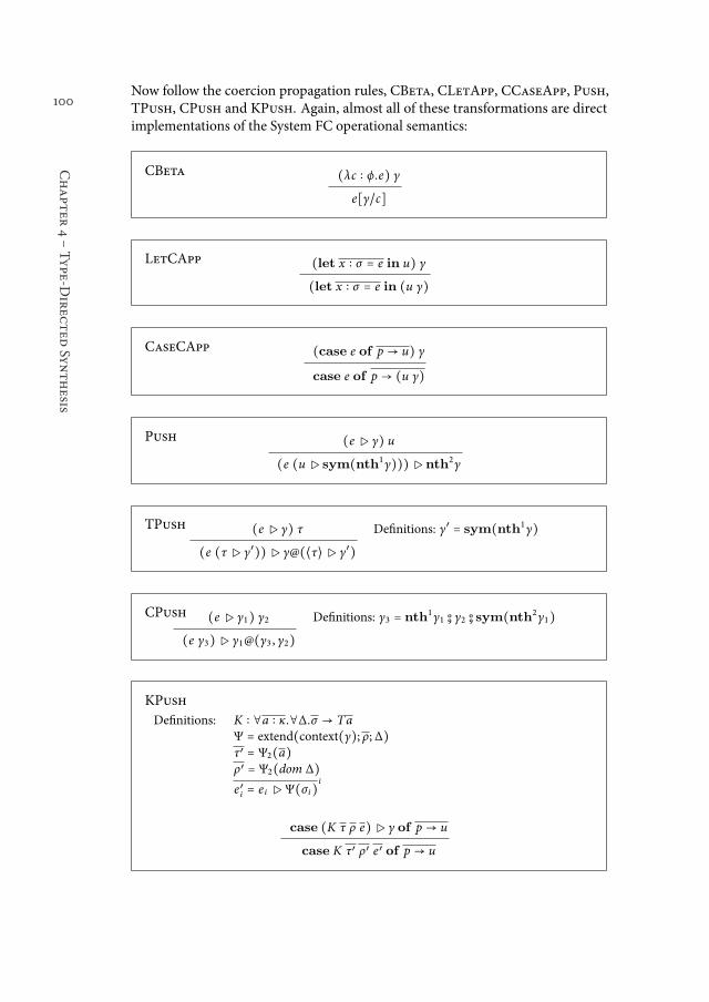
100

Chapter

4śType-D

irec

ted

Synthesis

Now follow the coercion propagation rules, CBeta, CLetApp, CCaseApp, Push,TPush, CPush and KPush. Again, almost all of these transformations are directimplementations of the System FC operational semantics:

CBeta (λc ∶ ϕ.e) γ

e∥γ/c∥

LetCApp (let x ∶ σ ≙ e in u) γ

(let x ∶ σ ≙ e in (u γ)

CaseCApp (case e of p → u) γ

case e of p → (u γ)

Push (e▷ γ) u

(e (u▷ sym(nth1γ)))▷ nth2γ

TPush (e▷ γ) τ Deinitions: γ′ ≙ sym(nth1γ)

(e (τ▷ γ′))▷ γ@(⟨τ⟩▷ γ′)

CPush (e▷ γ1) γ2 Deinitions: γ3 ≙ nth1γ1 o

9 γ2 o9 sym(nth

2γ1)

(e γ3)▷ γ1@(γ3 , γ2)

KPush

Deinitions: K ∶ ∀a ∶ κ.∀∆.σ → TaΨ ≙ extend(context(γ); ρ;∆)τ′ ≙ Ψ2(a)ρ′ ≙ Ψ2(dom ∆)

e′i ≙ e i ▷ Ψ(σi)i

case (K τ ρ e)▷ γ of p → u

case K τ′ ρ′ e′ of p → u

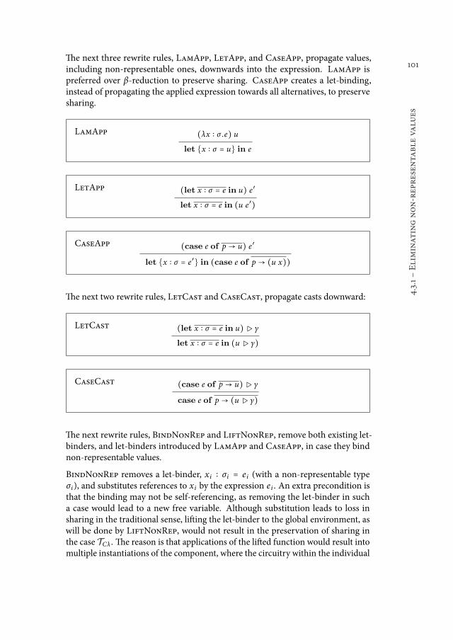
101

4.3.1śEliminat

ingnon-represen

table

valu

es

he next three rewrite rules, LamApp, LetApp, and CaseApp, propagate values,including non-representable ones, downwards into the expression. LamApp ispreferred over β-reduction to preserve sharing. CaseApp creates a let-binding,instead of propagating the applied expression towards all alternatives, to preservesharing.

LamApp (λx ∶ σ .e) u

let {x ∶ σ ≙ u} in e

LetApp (let x ∶ σ ≙ e in u) e′

let x ∶ σ ≙ e in (u e′)

CaseApp (case e of p → u) e′

let {x ∶ σ ≙ e′} in (case e of p → (u x))

he next two rewrite rules, LetCast and CaseCast, propagate casts downward:

LetCast (let x ∶ σ ≙ e in u)▷ γ

let x ∶ σ ≙ e in (u▷ γ)

CaseCast (case e of p → u)▷ γ

case e of p → (u▷ γ)

he next rewrite rules, BindNonRep and LiftNonRep, remove both existing let-binders, and let-binders introduced by LamApp and CaseApp, in case they bindnon-representable values.

BindNonRep removes a let-binder, x i ∶ σi ≙ e i (with a non-representable typeσi), and substitutes references to x i by the expression e i . An extra precondition isthat the binding may not be self-referencing, as removing the let-binder in sucha case would lead to a new free variable. Although substitution leads to loss insharing in the traditional sense, liting the let-binder to the global environment, aswill be done by LiftNonRep, would not result in the preservation of sharing inthe case TCλ . he reason is that applications of the lited function would result intomultiple instantiations of the component, where the circuitry within the individual

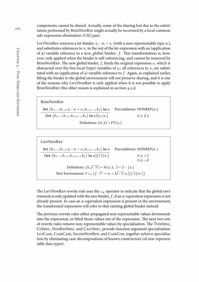
102

Chapter

4śType-D

irec

ted

Synthesis

components cannot be shared. Actually, some of the sharing lost due to the substi-tution performed by BindNonRepmight actually be recovered by a local commonsub-expression elimination (CSE) pass.

LiftNonRep removes a let-binder, x i ∶ σi ≙ e i (with a non-representable type σi),and substitutes references to x i in the rest of the let-expression with an (applicationof a) variable reference to a new, global, binder: f . his transformation is, how-ever, only applied when the binder is self-referencing, and cannot be removed byBindNonRep. he new global binder, f , binds the original expression e i which isabstracted over the free local (type) variables of e i ; all references to x i are substi-tuted with an (application of a) variable reference to f . Again, as explained earlier,liting the binder to the global environment will not preserve sharing, and it is oneof the reasons why LiftNonRep is only applied when it is not possible to applyBindNonRep (the other reason is explained in section 4.3.3).

BindNonRep

let {b1 ; ...; b i−1 ; x i ∶ σi ≙ e i ; b i+1 ; ...; bn} in u Preconditions: NONREP(σi)

(let {b1 ; ...; b i−1 ; b i+1 ; ...; bn} in u)∥e i/x i∥ ⋀ x i /∈ y

Deinitions: (a, y) ≙ FV(e i)

LiftNonRep

let {b1 ; ...; b i−1 ; x i ∶ σi ≙ e i ; b i+1 ; ...; bn} in u Preconditions: NONREP(σi )

(let {b1 ; ...; b i−1 ; b i+1 ; ...; bn} in u)∥ f z/x i∥ ⋀ x i ∈ y

⋀ a ≙ ∅

Deinitions: (a, y ∶ τ′) ≙ fv(e i); z ≙ y − {x i}

New Environment: Γ ∪α { f ∶ τ′ → σi ≙ λz ∶ τ′ .e i∥( f z)/x i∥}

he LiftNonRep rewrite rule uses the ∪α operator to indicate that the global envi-ronment is only updated with the new binder, f , if an α-equivalent expression is notalready present. In case an α-equivalent expression is present in the environment,the transformed expression will refer to that existing global binder instead.

he previous rewrite rules either propagated non-representable values downwardsinto the expression, or lited those values out of the expression. he next two setsof rewrite rules remove non-representable values by specialisation. he TypeSpec,CoSpec, NonRepSpec, and CastSpec, provide function argument specialisation.LetCase, CaseCase, InlineNonRep, and CaseCon, together achieve specialisa-tion by eliminating case-decompositions of known constructors (of non-represen-table data types).

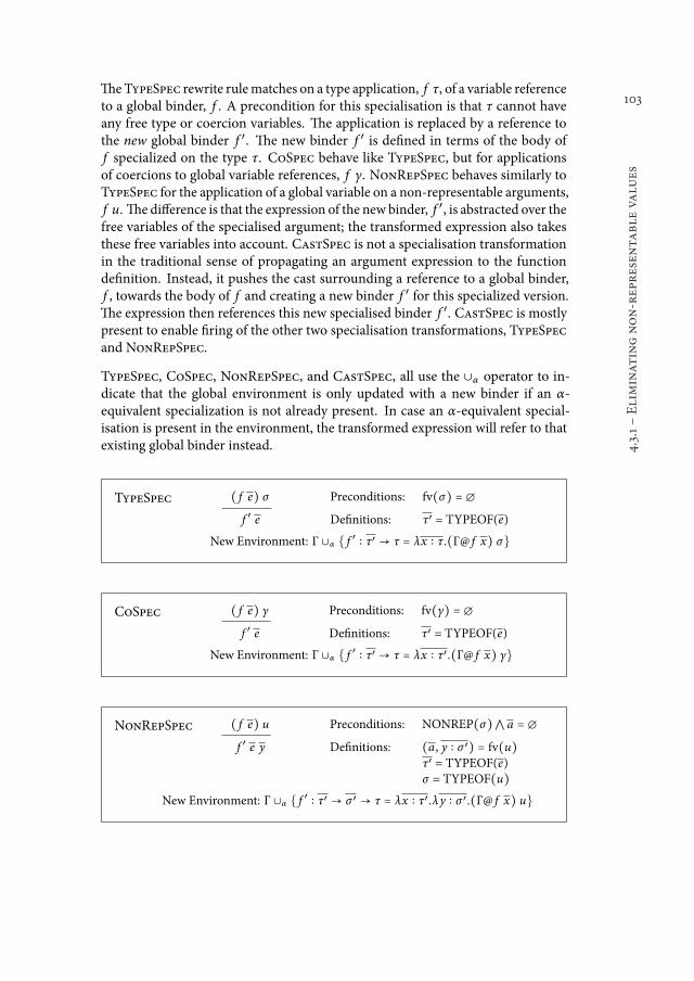
103

4.3.1śEliminat

ingnon-represen

table

valu

es

heTypeSpec rewrite rulematches on a type application, f τ, of a variable referenceto a global binder, f . A precondition for this specialisation is that τ cannot haveany free type or coercion variables. he application is replaced by a reference tothe new global binder f ′. he new binder f ′ is deined in terms of the body off specialized on the type τ. CoSpec behave like TypeSpec, but for applicationsof coercions to global variable references, f γ. NonRepSpec behaves similarly toTypeSpec for the application of a global variable on a non-representable arguments,f u. he diference is that the expression of the new binder, f ′, is abstracted over thefree variables of the specialised argument; the transformed expression also takesthese free variables into account. CastSpec is not a specialisation transformationin the traditional sense of propagating an argument expression to the functiondeinition. Instead, it pushes the cast surrounding a reference to a global binder,f , towards the body of f and creating a new binder f ′ for this specialized version.he expression then references this new specialised binder f ′. CastSpec is mostlypresent to enable iring of the other two specialisation transformations, TypeSpecand NonRepSpec.

TypeSpec, CoSpec, NonRepSpec, and CastSpec, all use the ∪α operator to in-dicate that the global environment is only updated with a new binder if an α-equivalent specialization is not already present. In case an α-equivalent special-isation is present in the environment, the transformed expression will refer to thatexisting global binder instead.

TypeSpec ( f e) σ Preconditions: fv(σ) ≙ ∅

f ′ e Deinitions: τ′ = TYPEOF(e)

New Environment: Γ ∪α { f′ ∶ τ′ → τ ≙ λx ∶ τ.(Γ@ f x) σ}

CoSpec ( f e) γ Preconditions: fv(γ) ≙ ∅

f ′ e Deinitions: τ′ = TYPEOF(e)

New Environment: Γ ∪α { f′ ∶ τ′ → τ ≙ λx ∶ τ′ .(Γ@ f x) γ}

NonRepSpec ( f e) u Preconditions: NONREP(σ)⋀ a ≙ ∅

f ′ e y Deinitions: (a, y ∶ σ ′) ≙ fv(u)τ′ = TYPEOF(e)σ = TYPEOF(u)

New Environment: Γ ∪α { f′ ∶ τ′ → σ ′ → τ ≙ λx ∶ τ′ .λy ∶ σ ′ .(Γ@ f x) u}

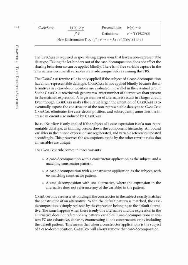
104

Chapter

4śType-D

irec

ted

Synthesis

CastSpec ( f e) ▷ γ Preconditions: fv(γ) ≙ ∅

f ′ e Deinitions: τ′ = TYPEOF(e)

New Environment: Γ ∪α { f′ ∶ τ′ → τ ≙ λx ∶ τ′ .(Γ@ f x)▷ γ}

he LetCase is required in specialising expressions that have a non-representabledatatype. Taking the let-binders out of the case-decomposition does not afect thesharing behaviour so can be applied blindly. here is no free variable capture in thealternatives because all variables are made unique before running the TRS.

he CaseCase rewrite rule is only applied if the subject of a case-decompositionhas a non-representable datatype. CaseCase is not applied blindly because the al-ternatives in a case-decomposition are evaluated in parallel in the eventual circuit.So theCaseCase rewrite rule generates a larger number of alternatives than presentin thematched expression. A larger number of alternatives results in a larger circuit.Even though CaseCasemakes the circuit larger, the intention of CaseCase is toeventually expose the constructor of the non-representable datatype to CaseCon.CaseCon eliminates the case-decomposition, and subsequently amortizes the in-crease in circuit size induced by CaseCase.

InlineNonRep is only applied if the subject of a case expression is of a non-repre-sentable datatype, as inlining breaks down the component hierarchy. All boundvariables in the inlined expression are regenerated, and variable references updatedaccordingly. his preserves the assumptions made by the other rewrite rules thatall variables are unique.

he CaseCon rule comes in three variants:

ż A case-decomposition with a constructor application as the subject, and amatching constructor pattern.

ż A case-decomposition with a constructor application as the subject, withnomatching constructor pattern.

ż A case-decomposition with one alternative, where the expression in thealternative does not reference any of the variables in the pattern.

CaseCon only creates a let-binding if the constructor in the subject exactlymatchesthe constructor of an alternative. When the default pattern is matched, the case-decomposition is simply replaced by the expression belonging to the default alterna-tive. he same happens when there is only one alternative and the expression in thealternative does not reference any pattern variables. Case-decompositions in Sys-tem FC are exhaustive, either by enumerating all the constructors, or by includingthe default pattern. his means that when a constructor applications is the subjectof a case-decomposition, CaseCon will always remove that case-decomposition.

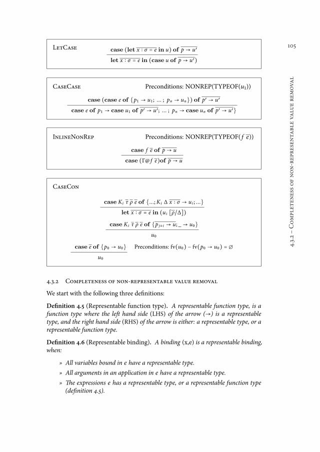
105

4.3.2śCompleten

essofnon-represen

table

valu

erem

ova

l

LetCase case (let x ∶ σ ≙ e in u) of p → u′

let x ∶ σ ≙ e in (case u of p → u′)

CaseCase Preconditions: NONREP(TYPEOF(u1))

case (case e of {p1 → u1 ; ... ; pn → un}) of p′ → u′

case e of p1 → case u1 of p′ → u′; ... ; pn → case un of p′ → u′}

InlineNonRep Preconditions: NONREP(TYPEOF( f e))

case f e of p → u

case (Γ@ f e)of p → u

CaseCon

case K i τ ρ e of {...;K i ∆ x ∶ σ → u i ; ...}

let x ∶ σ ≙ e in (u i ∥ρ/∆∥)

case K i τ ρ e of {p j≠i → u; _→ u0}

u0

case e of {p0 → u0} Preconditions: fv(u0) − fv(p0 → u0) ≙ ∅

u0

4.3.2 Completeness of non-representable value removal

We start with the following three deinitions:

Deinition 4.5 (Representable function type). A representable function type, is afunction type where the let hand side (LHS) of the arrow (→) is a representabletype, and the right hand side (RHS) of the arrow is either: a representable type, or arepresentable function type.

Deinition 4.6 (Representable binding). A binding (x,e) is a representable binding,when:

ż All variables bound in e have a representable type.

ż All arguments in an application in e have a representable type.

ż he expressions e has a representable type, or a representable function type(deinition 4.5).

106

Chapter

4śType-D

irec

ted

Synthesis

Deinition 4.7 (Representable environment). A representable environment is a clo-sed environment where every binding is a representable binding.

he irst set of rewrite rules (TBeta - LiftNonRep) propagate or remove non-representable values for those syntactical elements on which the specialisationrewrite rules do not match. he second set of rewrite rules (TypeSpec - CaseCon)remove the non-representable values through specialisation. he two sets of rewriterules ensure that the resulting environment of the normalisation phase is a repre-sentable environment (deinition 4.7), given the restrictions in Section 4.3.1.

he restrictions on primitives are needed because those cannot be specialized ontheir argument, nor can their deinitions be inlined. he restriction that the resulttype ofmain cannot be a non-representable data type, ensures that any expressioncalculating a non-representable data type always becomes the subject of a case-decomposition, which will be removed by the TRS.

his section will prove the following two theorems, which together ensure that,when the normalisation inishes, the resulting environment is a representable envi-ronment.

heorem: 4.3.1 (Representable bindings). When the main function, and all usedprimitives have representable (function) types then, given a binding (x,e), (x,e) iseither a representable binding, or one of the rewrite rules applies to e.

heorem: 4.3.2 (Representable environment). Given a closed environment Γ, anenvironment of representable bindings Γr , and a binding (x,e). Let (e’,Γ′) be the re-sulting tuple of exhaustively applying all the rewrite rules to e and Γ, and let Γ′r ≙Γr ∪ {(x , e′)}. hen (x,e’) is a representable binding; and Γ′r is a representable en-vironment or normalisation continues with Γ′, Γ′r , and the binders corresponding tothe free variables in Γ′r .

Notation

In order to give structure to the proofs of the above theorems we introduce a no-tation to represent all possible expressions. We will model expressions (not typesor coercions) in System FC as a set of syntax trees. We do this, so that ater everylemma, or in intermediate parts of a proof, we can show how that the set of all pos-sible expressions ater applying the rewrite rules exhaustively become smaller. Wewill ultimately end up with a set of possible expressions where our will theoremshold, thus having inished our proof.

We start with the deinitions of a few basic sets. here is the set V which representsall local variables, those not bound in the environment, and the set F which repre-sents all global variables, those bound in the environment. Next we have P , the setof primitives, K, the set of data constructors, T , the set of types, and C, the set ofcoercions. For the purpose behind our notation, to give structure to the proofs, itis not necessary to specify how these sets are generated.

107

4.3.2śCompleten

essofnon-represen

table

valu

erem

ova

l

Next we deine our set generators, which can generate certain sets of expressions.Notice that most are parametrized in the sets from which they can draw elements.

lam x = {λy ∶ τ.e ∣ y ∈ V , τ ∈ T , e ∈ x}app x y = {e u ∣ e ∈ x , u ∈ y}tyLam x = {Λa ∶ κ.e ∣ a ∈ V , κ ∈ T , e ∈ x}tyApp x = {e τ ∣ e ∈ x , τ ∈ T }coLam x = {λc ∶ ϕ.e ∣ c ∈ V , ϕ ∈ C , e ∈ x}coApp x = {e γ ∣ e ∈ x , γ ∈ C}prim = Pcon =Kvar = Vfun = Flet x y = {let v ∶ τ ≙ e in u ∣ v ⊆ V , τ ⊆ T , e ⊆ x , u ∈ y}case x y = {case e of p → u

+∣ e ∈ x , p ⊆ {_} ∪ pat, u ⊆ y}

pat = {K ∆ x ∶ σ ∣ K ∈ K, ∆ ⊆ tele, x ⊆ V , τ ⊆ T }tele = {a ∶ κ ∣ a ∈ V , κ ∈ T } ∪ {c ∶ ϕ ∣ c ∈ V , ϕ ∈ C}cast x = {e▷ γ ∣ e ∈ x , γ ∈ C}

We deine three derived set generators which we use to model nested application:

app∗ x y = {e u ∣ e ∈ (x − app x y), u ⊆ y}tyApp∗x = {e τ ∣ e ∈ (x − tyApp x y), tau ⊆ T }coApp∗x = {e γ ∣ e ∈ (x − coApp x y), tau ⊆ C}

where the LHS of the nested application is not itself that speciic kind of application.So app∗ x y, generates all nested term applications from expressions drawn fromthe sets x and y, but not the expressions in x that are themselves term applications;but it will, for example, generate a nested term application of a type application.

Note that we have not included a set generator for projections. he reason is thatprojections are only introduced by the second pass of the normalisation phase.Projections do not occur in the expressions generated by the front-end, nor do ourrewrite rules for non-representable value elimination introduce projections.

he set of expressions we can possibly create is the ixed point of the equation:S0 ≙ lam S0 ∪ app

∗ S0 S0 ∪ tyLam S0 ∪ tyApp∗ S0 ∪ coLam S0 ∪ coApp

∗ S0 ∪prim ∪ con ∪ var ∪ fun ∪ let S0 S0 ∪ case S0 S0 ∪ cast S0

For every lemma n and its corresponding proof, we will deine a new set of expres-sion, Sn , that are possible under the restrictions of the lemma. Every subsequentset of possible expressions is a proper subset of the previous set, that is, Sn ⊃ Sn+1.

108

Chapter

4śType-D

irec

ted

Synthesis

Proof of the theorems

For our proofs of theorem 4.3.1 and theorem 4.3.2, wewill irst need to deine severallemmas.

Lemma: 4.3.1 (Correctly typed). Expressions are correctly typed. herefore:

1. he subject of a case-decomposition is not an abstraction.

2. Term-abstractions are never the subject of a type- or coercion-application.

3. Type-abstractions are never the subject of a term- or coercion-application.

4. Coercion-abstractions are never the subject of a term- or type-application.

5. Constructors are irst applied to their type and coercion arguments, beforethey are applied to their term arguments.

6. By the well-formedness check (appendix C), primitives are monomorphic.

Proof. he original expression is correctly typed and all of our transformationspreserve correct typing.

We deine our new set of possible expressions under the restrictions set by thelemma as:

S1 ≙ lam S1 ∪ app∗ (S1 − tyLam S1 − coLam S1) S1 ∪ tyLam S1 ∪ tyApp∗ A1 ∪coLam S1 ∪ coApp∗ B1 ∪ prim ∪ con ∪ var ∪ fun ∪ let S1 S1 ∪ case (S1 −lam S1 − tyLam S1 − coLam S1) S1 ∪ cast S1

A1 ≙ app∗ (S1 −prim− con− tyLam S1 − coLam S1) S1 ∪ tyLam S1 ∪ coApp∗ B1 ∪

con ∪ var ∪ fun ∪ let S1 S1 ∪ case (S1− lam S1−tyLam S1−coLam S1) S1∪ cast S1

B1 ≙ app∗ (S1 −prim− con− tyLam S1 − coLam S1) S1 ∪ tyApp∗ A1 ∪ coLam S1 ∪

con ∪ var ∪ fun ∪ let S1 S1 ∪ case (S1− lam S1−tyLam S1−coLam S1) S1∪ cast S1

For readability, we have deined two new subsets,A1 and B1, to represent the pos-sible expressions that can form the LHS of a type application (A1) or the LHS of acoercion application (B1).

Lemma: 4.3.2 (Only constructor, variable, function, and primitive applications).here are only type- and coercion-applications of constructors and of (applicationsof) local variables. here are only term-applications of: global functions, primitives,constructors, local variables, and of the earlier mentioned type- and coercion-applica-tions.

Proof. By enumerating all the other possible locations for type-, coercion-, andterm-applications in S1, and showing that they are removed by one of the transfor-mations.

109

4.3.2śCompleten

essofnon-represen

table

valu

erem

ova

l

ż An application of a term-abstractions is removed by LamApp.

ż An application of a let-expressions is removed by the LetApp.

ż An application of a case-decomposition is removed by CaseApp.

ż An application of a cast is removed by Push

ż Types applied to type-abstractions are propagated by TBeta.

ż Types applied to global functions are propagated by TypeSpec.

ż Types applied to let-expressions are propagated by LetTApp.

ż Types applied to case-decompositions are propagated by CaseTApp.

ż Types applied to casts are removed by TPush.

ż Coercions applied to coercion-abstractions are propagated by CBeta.

ż Coercions applied to global functions are propagated by CoSpec.

ż Coercions applied to let-expressions are propagated by LetCApp.

ż Coercions applied to case-decompositions are propagated by CaseCApp.

ż Coercions applied to casts are removed by CPush.

hus, our new set of possible expressions possible under the lemma, is deined by:

S2 ≙ lam S2 ∪ app∗ (prim ∪ con ∪ var ∪ fun ∪ tyApp∗ A2 ∪ coApp∗ B2) S2 ∪tyLam S2 ∪ tyApp∗ A2 ∪ coLam S2 ∪ coApp∗ B2 ∪ prim ∪ con ∪ var ∪ fun ∪let S2 S2 ∪ case (S2 − lam S2 − tyLam S2 − coLam S2) S2 ∪ cast S2

A2 ≙ app∗ var S2 ∪ coApp∗ B2 ∪ con ∪ var

B2 ≙ app∗ var S2 ∪ tyApp∗ A2 ∪ con ∪ var

Note that we still deine subsets for the LHSs of type and coercion applications.

Deinition 4.8 (Representable set). We deine Rn as the set of expressions drawnfrom Sn whose type is representable.

Lemma: 4.3.3 (Representable arguments). he arguments of an application of aprimitive or of a global function are representable.

Proof. he precondition states that all arguments to primitives must have a re-presentable type. Non-representable arguments applied to global functions arepropagated by NonRepSpec.

110

Chapter

4śType-D

irec

ted

Synthesis

Our new set of possible expressions is:

S3 ≙ lam S3 ∪ app∗ (con ∪ var ∪ tyApp∗ A2 ∪ coApp∗ B2) S3 ∪ app∗ (prim ∪fun)R3 ∪ tyLam S3 ∪ tyApp∗ A2 ∪ coLam S3 ∪ coApp∗ B2 ∪ prim ∪ con ∪var ∪ fun ∪ let S3 S3 ∪ case (S3 − lam S3 − tyLam S3 − coLam S3) S3 ∪ cast S3

A3 ≙ app∗ var S3 ∪ coApp∗ B3 ∪ con ∪ var

B3 ≙ app∗ var S3 ∪ tyApp∗ A3 ∪ con ∪ var

Lemma: 4.3.4 (Representable let-bindings). All let-bindings are representable.

Proof. Let-bindings with a type that is not representable are either inlined by Bind-NonRep, or turned into a global function by LiftNonRep.

Our new set of expressions still possible under the lemma is:

S4 ≙ lam S4 ∪ app∗ (con ∪ var ∪ tyApp∗ A2 ∪ coApp∗ B2) S4 ∪ app∗ (prim ∪fun)R4 ∪ tyLam S4 ∪ tyApp∗ A2 ∪ coLam S4 ∪ coApp∗ B2 ∪ prim ∪ con ∪var ∪ fun ∪ letR4 S4 ∪ case (S4 − lam S4 − tyLam S4 − coLam S4) S4 ∪ cast S4

A4 ≙ app∗ var S4 ∪ coApp∗ B4 ∪ con ∪ var

B4 ≙ app∗ var S4 ∪ tyApp∗ A4 ∪ con ∪ var

henext two lemmas, lemma 4.3.5 and lemma 4.3.6, form a bi-implication. he irstlemma, lemma 4.3.5, shows that ater all transformations have been applied exhaus-tively, all remaining pattern-bound variables are representable. he second lemma,lemma 4.3.6, shows that ater all transformations have been applied exhaustively,all remaining lambda-bound variables are representable. As these lemmas form abi-implication we will deine our new set of possible expressions in corollary 4.3.1which follows the two lemmas.

Lemma: 4.3.5 (Representable pattern-binders). If there are only representablelambda-binders, then the subjects of case-decompositions are representable.

Proof. Case-decompositions with an (application of a) constructor are removedby CaseCon. We thus show that, when the subject of a case-decomposition has anon-representable type, then the subject always becomes a constructor application.We only enumerate then cases still allowed by S4:

ż (Applications of) global functions are inlined by InlineNonRep

111

4.3.2śCompleten

essofnon-represen

table

valu

erem

ova

l

ż Let-expressions will have their let-bindings extracted by CaseLet, leavingonly the body.

ż Case-decompositions have their alternatives propagated to the alternativesof the encompassing case-decomposition by CaseCase.

ż Regarding casts:

ś Casts of (applications of) global functions are propagated by Cast-Spec.

ś Casts of (applications of) constructors are propagated by KPush.ś Casts of let-expressions are propagated by LetCast.ś Casts of case-decompositions are propagated by CaseCast.

ż Regarding (applications or casts of) local variables:

ś By the precondition, it cannot be a lambda-bound variable, as it wouldbe non-representable.

ś It cannot be a pattern-bound variable, as that would imply that thesubject of a case-decomposition has a non-representable type. By theinduction hypothesis, those case-decompositions have already beenremoved by CaseCon.

Lemma: 4.3.6 (Representable lambda-bindings). If there are only case-decomposi-tions with representable subjects, then all lambda-binders are representable.

Proof. he normalisation process proceeds in a top-down traversal of the functionhierarchy, starting with the main function. We prove, by induction, that term-abstraction with a non-representable binder no longer exist:

ż We are normalising themain function:

ś By the precondition on normalisation,main has a representable func-tion type.

ś hepossible locations for a term-abstraction with a non-representablebinder still possible in S4 are: as an argument of a constructor or alocal variable application.

ś However, a constructor with a non-representable argument is itselfnon-representable. By the precedent of the lemma, that subjects ofcase-decompositions are representable, so the non-representable con-structor application can also only occur as an argument to a construc-tor or variable application.

ś Because subjects of case-decompositions are representable, there arehowever no pattern-bound variables that can be the LHS of an appli-cation.

ś When a lambda-bound variable is the LHS of an application, then theterm-abstraction which introduces the binder can also only exists asan argument to an application.

112

Chapter

4śType-D

irec

ted

Synthesis

ś Becausemain has a representable function type, the above mentionedapplication do not exist.

ż We are normalising a function other thanmain:

ś he type of the expression must be a representable (function) type.Otherwise the expression would have been inlined by InlineNonRep,or it would have entailed that the callers in the function hierarchy, andultimatelymain would have had a non-representable (function) type.

ś he expressions has a representable (function) type; by lemma 4.3.3the expression is specialised on all non-representable argument. Anyterm-abstraction that would have contributed to a non-representa-ble function type has thus become the subject of an application. Bylemma 4.3.2, those applications are removed, as witnessed by the pos-sible expressions we can draw from S4.

ś Following the same reasoning as for the normalisation ofmain, term-abstractions with a non-representable type cannot occur anywhereelse.

Corollary: 4.3.1 (No variable applications). Applications of local variables are re-moved, and all bound variables are representable.

Proof. Lemma 4.3.5 proves that, if there are only representable lambda-binders,then the subjects of case-decompositions are representable. Lemma 4.3.6 provesthat, if there are only case-decompositions with representable subjects, then alllambda-binders are representable. From lemma 4.3.5 we can derive that all pattern-bound variables are representable.

Lemmas 4.3.4, 4.3.5, and 4.3.6 together show that all bound variables are represen-table. his entails that there are no local variables with a polymorphic or functiontype.

Our new set of expressions still possible under the corollary is:

S5 ≙ lamS5 ∪ app∗ (con ∪ tyApp∗A5∪ coApp

∗ B5)S5 ∪ app∗ (prim ∪ fun)R5 ∪

tyLam S5 ∪ tyApp∗ A5 ∪ coLam S5 ∪ coApp∗ B5 ∪ prim ∪ con ∪ var ∪ fun ∪let R5 S5 ∪ caseR5 S5 ∪ cast S5

A5 ≙ coApp∗ B5 ∪ con

B5 ≙ tyApp∗ A5 ∪ con

Deinition 4.9 (Type- and coercion-applied constructor). We deine a new set gen-erator which we use to model constructors applied to types and coercions:

113

4.3.2śCompleten

essofnon-represen

table

valu

erem

ova

l

con∆ = {K τ ρ ∣ K ∈ K, τ ⊆ T , ρ ⊆ (T ∪ C)}

We can now remove the explicit type and coercion applications from our possibleset of expressions and redeine S5 as:

S5 ≙ lam S5 ∪ app∗ con∆ S5 ∪ app∗ (prim ∪ fun)R5 ∪ tyLam S5 ∪ coLam S5 ∪prim ∪ con∆ ∪ var ∪ fun ∪ let R5 S5 ∪ caseR5 S5 ∪ cast S5

Lemma: 4.3.7 (No type- or coercion-abstractions). All type-abstractions and allcoercion-abstractions are removed.

Proof. he normalisation process proceeds in a top-down traversal of the functionhierarchy, starting with the main function. We prove, by induction, that type-ab-stractions and coercion-abstractions no longer exist:

ż We are normalising themain function:

ś By the precondition on normalisation,main has a representable func-tion type.

ś he only possible location where type- and coercion-abstraction arestill possible in S5, are as arguments in a constructor application.

ś hose constructor applications would themselves be non-representa-ble, and can also only exists as arguments in a constructor application.

ś Becausemain has representable function type, those applications donot exist.

ż We are normalising a function other thanmain:

ś he type of the expression must be a representable (function) type.Otherwise the expression would have been inlined by InlineNonRep,or it would have entailed that the callers in the function hierarchy, andultimatelymain would have had a non-representable (function) type.

ś he expressions has a representable (function) type; by lemma 4.3.3the expression is specialised on all type and coercion arguments. Anytype- or coercion-abstraction that would have contributed to a non-representable function type have thus become the subject of a type- orcoercion-application. By lemma 4.3.2, those applications are removed,as witnessed by the possible expressions we can draw from S5.

ś Following the same reasoning as for the normalisation ofmain, type-abstractions and term-abstractions cannot occur anywhere else.

S6 ≙ lam S6 ∪ app∗ con∆ S6 ∪ app∗ (prim ∪ fun)R6 ∪ prim ∪ con ∪ var ∪fun ∪ let R6 S6 ∪ caseR6 S6 ∪ cast S6

We now recapitulate our two theorems, theorem 4.3.1 and theorem 4.3.2, and provethem with using our lemmas. Recall deinition 4.6:

114

Chapter

4śType-D

irec

ted

Synthesis

Deinition 4.6 (Representable binding). A binding (x,e) is a representable binding,when:

ż All variables bound in e have a representable type.

ż All arguments in an application in e have a representable type.

ż he expressions e has a representable type, or a representable function type(deinition 4.5).

heorem: 4.3.1 (Representable bindings). When the main function, and all usedprimitives have representable (function) types then, given a binding (x,e), (x,e) iseither a representable binding, or one of the rewrite rules applies to e.

Proof. Combining lemmas 4.3.1 - 4.3.7 and corollary 4.3.1 we arrive at a set of pos-sible expression forms, S6, when all rewrite rules have been exhaustively applied.In S6, all bound variables have a representable type (corollary 4.3.1), and the argu-ments of a primitive application and global function application are representable.Constructors with non-representable arguments are themselves non-representable.he normalisation process proceeds in a top-down traversal of the function hier-archy, starting with themain function. We prove, by induction, that constructorswith non-representable arguments no longer exist:

ż We are normalising themain function:

ś By the precondition on normalisation,main has a representable func-tion type.

ś he only possible location where non-representable constructor arestill possible in S6, are as arguments in a constructor application.

ś hose constructor applications would themselves be non-representa-ble, and can also only exists as arguments in a constructor application.

ś Becausemain has representable function type, those applications donot exist.

ż We are normalising a function other thanmain:

ś he type of the expression must be a representable (function) type.Otherwise the expression would have been inlined by InlineNonRep,or it would have entailed that the callers in the function hierarchy, andultimatelymain would have had a non-representable (function) type.

ś Following the same reasoning as for the normalisation of main, con-structors with non-representable arguments cannot occur anywhereelse.

Our inal set of possible expressions is hence:

S7 ≙ lam S7 ∪ app∗ (con∆ ∪ prim ∪ fun)R7 ∪ prim ∪ con ∪ var ∪ fun ∪let R7 S7 ∪ caseR7 S7 ∪ cast S7

115

4.3.3śTer

minat

ionofnon-represen

table

valu

erem

ova

l

heorem: 4.3.2 (Representable environment). Given a closed environment Γ, anenvironment of representable bindings Γr , and a binding (x,e). Let (e’,Γ′) be the re-sulting tuple of exhaustively applying all the rewrite rules to e and Γ, and let Γ′r ≙Γr ∪ {(x , e′)}. hen (x,e’) is a representable binding; and Γ′r is a representable en-vironment or normalisation continues with Γ′, Γ′r , and the binders corresponding tothe free variables in Γ′r .

Proof. By theorem 4.3.1 exhaustively applying all the rewrite rules to an expressionin the binding (x,e) creates a realisable binding (x,e’). So Γ′r is also a set of realisablebinders. When Γ′r is closed, Γ

′r is a representable environment. When Γ′r is not

closed, the normalisation process will normalise the binders referenced in Γ′r butare themselves not in Γ′r .

Now that we have proven that the normalisation process produces a representableenvironment, under the precondition that main and all used primitives have a re-presentable function type, we will now move on to the termination aspects of thenon-representable value removal pass.

4.3.3 Termination of non-representable value removal

here are several (combinations of) rewrite rules that induce non-termination ofthe unconstrained TRS. he CλaSH compiler must therefore:

ż Apply the rewrite rules according to a speciic strategy.

ż Include termination measures.

When one of the termination measures is triggered, non-representable values re-main present in the description. TCλ will not be able to transform the descriptionto a netlist when that happens.

It should be noted that these termination measures are only trigged on functionsthat contain unbounded (mutually) recursive function calls, or have a (mutually)recursive data type as a result; functions which cannot be synthesized by TCλ any-way. It can hence be said that theCλaSH compiler can produce circuits for all usefulcircuit descriptions.

In the next three subsections we highlight where non-termination might occur,and how it is prevented. We will use Haskell instead of System FC, for purposesof brevity, to present expressions that can induce non-termination in the uncon-strained TRS.

Non-termination of InlineNonRep

Although inlining is already restricted to subjects of case decompositions that havea non-representable type, inlining can still cause non-termination. his happenswhen a recursive function call becomes the subject of a case decomposition:

116

Chapter

4śType-D

irec

ted

Synthesis

data B a = B af = case f of B _ → B (λx → x)

Where the type of f is data type with a ield that has a function value, which is anon-representable data type. When we now apply the transformation rules, we get:

case f of B _ → B (λx → x)⇒ InlineNonRep

case (case f of B _ → B (λx → x)) of B _ → B (λx → x)⇒ CaseCase

case f of B _ → (case B (λx → x) of B _ → B (λx → x))⇒ CaseCon

case f of B _ → B (λx → x)

Obviously this sequence of transformations will never terminate. Beside the factthat the expression is recursive, it also has a non-representable type, meaning itcould have never been transformed to an actual circuit.

If we were to use f in an expression where its result is never used internally, suchas:

main = λx → case f of B _ → x

hen the order in which the transformations are applied will determine if normal-isation terminates or not. If CaseCon is applied irst we will terminate with theexpression:

main = λx → x

However, if we delayed the application of the CaseCon rule, we might end up withthe following sequence of transformations:

λx → case f of B _ → x⇒ InlineNonRep

λx → case (case f of B _ → B (λx → x)) of B _ → x⇒ CaseCase

λx → case f of B _ → (case B (λx → x) of B _ → x)⇒ CaseCon

λx → case f of B _ → x

Resulting in a expression that will loop in the same way as the expression bound tof . To prevent such sequences from occurring we have adapted the strategy of ourTRS to apply the CaseCon transformation before InlineNonRep.

If f were bound in a let-expression, and the bound variable is not used inside theexpression, then the use of f will disappear from the function hierarchy throughLiftNonRep or BindNonRep. In case f is applied to a term abstraction where theabstracted variable is not used, then f will also disappear from the function hierar-chy through the combination of LamApp and, LiftNonRep or BindNonRep.

117

4.3.3śTer

minat

ionofnon-represen

table

valu

erem

ova

l

Additionally, although the TRS does not contain β-reduction as one of the rewriterules, LamApp, LiftNonRep, InlineNonRep, and CaseCon together behave likeβ-reduction. his means that the typed version of (λx → x x) (λx → x x):

data T = C (T → Int )(λx → case x of C h → h x) (C (λx → case x of C h → h x))

induces non-termination. To prevent this situation from happening, a function fcan only be inlined a inite number of times, where the amount of inlinings perfunction can be set by the user of the CλaSH compiler.

Non-termination of specialisation

A situation that would cause non-termination of NonRepSpec, is when the non-representable argument that will be propagated has local free variables with a non-representable type.

let x : Int → Int = λx: Int → x in f x⇒ NonRepSpec

let x : Int → Int = λx: Int → x in f ’ x⇒ NonRepSpec

let x : Int → Int = λx: Int → x in f ’ x⇒ NonRepSpec

let x : Int → Int = λx: Int → x in f ’ x

In this situation, the local free variable (which has a non-representable type) wouldalso be applied to the specialized function. heNonRepSpec transformationwouldthus specialize indeinitely as the local free variables, who have a non-representabletype, will remain applied to the specialized function. his is one of the reasonswhy the strategy of our TRS only applies the NonRepSpec transformation whenall the other transformations have already been exhaustively applied. When Non-RepSpec is applied last, all local free variables with a non-representable type arereplaced by either a global variable or a term-abstraction (through BindNonRepand LiftNonRep).

Another reason for non-termination as a result of NonRepSpec is when a recursivefunction f has an argument that accumulates non-representable values.

main = f idf :: ( Int → Int ) → Int → Intf g x = f ((+1) . g) x

Which ater the irst specialisation becomes:

main = f ’f :: ( Int → Int ) → Int → Intf g x = f ((+1) . g) x

f ’ x = f ((+1) . id ) x

118

Chapter

4śType-D

irec

ted

Synthesis

And ater another round of specialisation becomes:

main = f ’f :: ( Int → Int ) → Int → Intf g x = f ((+1) . g) x

f ’ x = f ’’ xf ’’ x = f ((+1) . ((+1) . id ) ) x

Which would lead to endless specialisations of f . To ensure termination, a Non-RepSpec is only applied to a function a inite number of times, where the amountof specialisation per function can be set by the user of the CλaSH compiler.

In a situation similar to the above, TypeSpec can induce non-termination whenspecialising polymorphic recursive functions such as:

1 data Nested a = a : ⟨ : (Nested [a]) | Epsilon2 inixr 5 : ⟨ :3

4 lengthN :: Nested a → Int5 lengthN Epsilon = 0

6 lengthN (_ : ⟨ : xs) = 1 + lengthN xs7

8 main :: Nested Int → Int9 main = lenghtN

Where lengthN, will irst be specialised on Int, ater that on [Int], ater that on [[Int]],and so on. So to ensure termination, not only NonRepSpec is equipped with atermination measure that limits the number of specialisations. All specialisationfunctions, NonRepSpec, TypeSpec, CoSpec, and CastSpec, are only applied ainite number of times.

Looping of NonRepSpec and LiftNonRep

We have already elaborated why applying BindNonRep is preferable above Lift-NonRep when possible. Below we show a situation why BindNonRep must beincluded to prevent non-termination.

he LiftNonRep transformation could induce non-termination in the presenceof recursion. Again, we want to highlight that unbounded recursion is not synthe-sisable to a digital circuit under our synthesis scheme TCλ . he following examplewill result in non-termination due to interactions between LiftNonRep andNon-RepSpec:

main = f notf = λa x → (a x) && (f a x)

In the irst iteration, we create a version of f specialized on not: f ′:

119

4.3.3śTer

minat

ionofnon-represen

table

valu

erem

ova

l

main = f ’f = λa x → (a x) && (f a x)f ’ = (λa x → a x && ( f a x)) not

When the TRS starts working on f ′, it will irst bind not to the variable a in alet-binding through LamApp.

main = f ’f = λa x → (a x) && (f a x)f ’ = let a = not in (λx → a x && (f a x))

he a binder is turned into a global variable g by LiftNonRep.

main = f ’f = λa x → (a x) && (f a x)f ’ = λx → g x && (f g x)g = not

he recursive call to f will now be specialized on g, to create a new version of fcalled f ′′.

main = f ’f = λa x → (a x) && (f a x)f ’ = λx → g x && (f ’’ x)g = notf ’’ = (λa x → (a x) && (f a x)) g

his process will continue indeinitely, as LiftNonRep will create a new globalvariable, meaning the specializations are not α-equivalent. Specialization wouldtherefore generate an ininite number of specializations of f .

his is the reason that LiftNonRep only works for self-referencing let-binders, andBindNonRep is used for all the others. When the set of functions has the form:

main = f ’f ’ = let a = not in (λx → a x && (f a x))f = λa x → (a x) && (f a x)

Instead of creating a new function g, the function not is simply inlined by Bind-NonRep in f ′.

main = f ’f ’ = λx → not x && (f not x)f = λa x → (a x) && (f a x)

Specialization will in this case not create a new function f ′′, because the specialisa-tion of f on not has been seen before.

120

Chapter

4śType-D

irec

ted

Synthesis

main = f ’f ’ = λx → not x && (f ’ x)f = λa x → (a x) && (f a x)

Strategy

We have seen that the unconstrained TRS can induce non-termination, and thatin some cases extra termination measures have to be implemented in the CλaSHcompiler. Other forms of non-termination could be induced by picking the trans-formations in the wrong order. We thus apply the transformations in a speciicorder. We classify our transformations in three groups:

Argument specialisation: hese transformations specialise top-level functions ontheir argument, which are: TypeSpec, CoSpec, and NonRepSpec.

Inlining: hese transformations inline top-level functions, which is only the Inli-neNonRep transformation.

Propagation: hese transformations propagate informations downwards into theexpression, and includes all the transformations not mentioned above.

he strategy that we employ is the following:

1. Apply the propagation transformations in an inner-most traversal.

2. Apply the inlining transformations in a bottom-up traversal, if these succeed,run step 1 again.

3. Apply the specialisations transformations in a bottom-up traversal.

Neither the correctness of the individual transformations, nor the guarantee ofa normal form, are dependent on this speciic ordering of transformations. heargument-specialisation rewrite rules are applied last, so that the fewest numberof new functions is introduced, and the original function hierarchy is preservedas much as possible. Because specialisation transformations do not create expres-sions on which the other rewrite rules match, all rewrite rules have been appliedexhaustively ater the traversal with specialisation transformations. he CastSpectransformation is included in the propagation transformations, and not the spe-cialisation transformations, because it enables irings of InlineNonRep. PuttingCastSpec in the propagations transformations is hence required in order to guar-antee the normal form.

4.3.4 Simplification

he normal form that facilitates a trivial translation to a netlist is repeated in ig-ure 4.15. A top-level expression, t , is single let-expression with a variable referenceas a body; it is possibly λ-abstracted over its arguments. he bindings of the let-expression are all in administrative normal form (ANF).

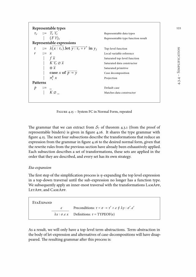
121

4.3.4śSimplificat

ion

Representable typesτr ::= Tr τr Representable data types

∣ (F τ)r Representable type function result

Representable expressions

t ::= λ(x ∶ τr).let y ∶ τr ≙ r+in y j Top-level function

r ::= x Local variable reference

∣ f x Saturated top-level function

∣ K τr ∅ x Saturated data constructor

∣ ⊗ x Saturated primitive

∣ case x of p → y Case decomposition

∣ πki x Projection

Patternsp ::= _ Default case

∣ K ∅ _ Matches data constructor

Figure 4.15 ś System FC in Normal Form, repeated

he grammar that we can extract from S7 of theorem 4.3.1 (from the proof ofrepresentable binders) is given in igure 4.16. It shares the type grammar withigure 4.15. he next four subsections describe the transformations that reduce anexpression from the grammar in igure 4.16 to the desired normal form, given thatthe rewrite rules from the previous section have already been exhaustively applied.Each subsection describes a set of transformations, these sets are applied in theorder that they are described, and every set has its own strategy.

Eta-expansion

he irst step of the simpliication process is η-expanding the top level expressionin a top-down traversal until the sub-expression no longer has a function type.We subsequently apply an inner-most traversal with the transformations LamApp,LetApp, and CaseApp.

EtaExpand

e Preconditions: τ ≙ σ → τ′ ∧ e /≙ λy ∶ σ ′ .e′

λx ∶ σ .e x Deinitions: τ = TYPEOF(e)

As a result, we will only have a top-level term-abstractions. Term-abstraction inthe body of let-expression and alternatives of case-decompositions will have disap-peared. he resulting grammar ater this process is:

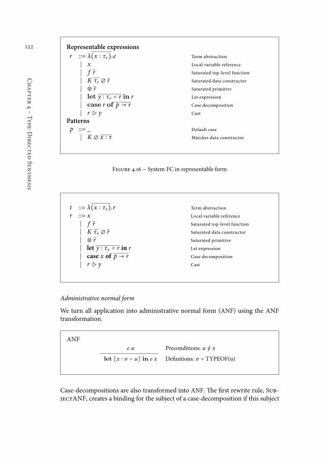
122

Chapter

4śType-D

irec

ted

Synthesis

Representable expressions

r ::= λ(x ∶ τr).e Term abstraction

∣ x Local variable reference

∣ f r Saturated top-level function

∣ K τr ∅ r Saturated data constructor

∣ ⊗ r Saturated primitive

∣ let y ∶ τr ≙ r in r Let expression

∣ case r of p → r Case decomposition

∣ r▷ γ Cast

Patternsp ::= _ Default case

∣ K ∅ x ∶ τ Matches data constructor

Figure 4.16 ś System FC in representable form

t ::= λ(x ∶ τr).r Term abstraction

r ::= x Local variable reference

∣ f r Saturated top-level function

∣ K τr ∅ r Saturated data constructor

∣ ⊗ r Saturated primitive

∣ let y ∶ τr ≙ r in r Let expression

∣ case x of p → r Case decomposition

∣ r▷ γ Cast

Administrative normal form

We turn all application into administrative normal form (ANF) using the ANFtransformation.

ANF

e u Preconditions: u /≙ x

let {x ∶ σ ≙ u} in e x Deinitions: σ = TYPEOF(u)

Case-decompositions are also transformed into ANF. he irst rewrite rule, Sub-jectANF, creates a binding for the subject of a case-decomposition if this subject

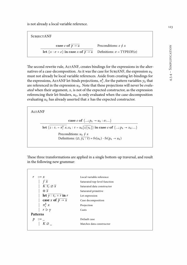
123

4.3.4śSimplificat

ion

is not already a local variable reference.

SubjectANF

case e of p → u Preconditions: e /≙ x

let {x ∶ σ ≙ e} in case x of p → u Deinitions: σ = TYPEOF(e)

he second rewrite rule, AltANF, creates bindings for the expressions in the alter-natives of a case-decomposition. As it was the case for SubjANF, the expression uk

must not already be local variable references. Aside from creating let-bindings forthe expressions,AltANF let-binds projections, πk

i , for the pattern variables yk thatare referenced in the expression uk . Note that these projections will never be evalu-ated when their argument, x, is not of the expected constructor, as the expressionreferencing their let-binders, uk , is only evaluated when the case-decompositionevaluating uk has already asserted that x has the expected constructor.

AltANF

case e of {...; pk → uk ∶ σ ; ...}

let {z ∶ τ i ≙ πki x; xk ∶ τ ≙ uk∥z/yk∥} in case e of {...; pk → xk ; ...}

Preconditions: uk /≙ xDeinitions: (∅, yk ∶ τ) = fv(uk) - fv(pk → uk)

hese three transformations are applied in a single bottom-up traversal, and resultin the following new grammar:

r ::= x Local variable reference

∣ f x Saturated top-level function

∣ K τr ∅ x Saturated data constructor

∣ ⊗ x Saturated primitive

∣ let y ∶ τr ≙ r in r Let expression

∣ case x of p → x Case decomposition

∣ πki x Projection

∣ r▷ γ Casts

Patternsp ::= _ Default case

∣ K ∅ _ Matches data constructor

124

Chapter

4śType-D

irec

ted

Synthesis

Let-simpliication

he next three transformations ensure that the body of a let-expression is a local vari-able reference, and none of the bound-expressions are themselves a let-expression.he irst transformation, bodyVar, ensures that the (representable) body of a let-expression is always a local variable reference. We have already seen the secondtransformation, LetCast, in the non-representable value elimination pass. It en-sures that casts are propagated towards the body of a let-expressions, and is neededfor the third rewrite rule to ire. he third transformation, LetFlat, inally ensuresthat nested let-expressions are turned into a single let-expression.

BodyVar

let x ∶ σ ≙ u in e Preconditions: e /≙ x

let {x ∶ σ ≙ u, xn+1 ∶ τ ≙ e} in xn+1 Deinitions: τ = TYPEOF(e)

LetCast (let x ∶ σ ≙ u in e)▷ γ

let x ∶ σ ≙ u in (e▷ γ)

LetFlat let {b1 ; ...; b i−1 ; x i ∶ σi ≙ let x ∶ σ ≙ u in e i ; b i+1 ; ...; bn} in u

let {b1 ; ...; b i−1 ; x ∶ σ ≙ u; x i ∶ σi ≙ e i ; b i+1 ; ...; bn} in u

he above three transformations are applied using a single bottom-up traversal.he inal rewrite rule, TopLet, ensures that the expression following the top-levelterm-abstractions is always a let-expression. As we did for EtaExpand, TopLet isapplied in a top-down traversal until the sub-expression no longer has a functiontype.

TopLet e Preconditions: (e /≙ let y ∶ σ in z) ∧ (τ /≙ σ → τ′)

let {x ∶ τ ≙ e} in x Deinitions: τ = TYPEOF(e)

We inally arrive at the grammar given in igure 4.17.

Remaining casts

When looking at the last grammar given in igure 4.17, it almost matches the gram-mar in igure 4.15, with the exception of the casts. Coercions witness a non-syntac-tical equality between types. Consequently, both the coerced and uncoerced value

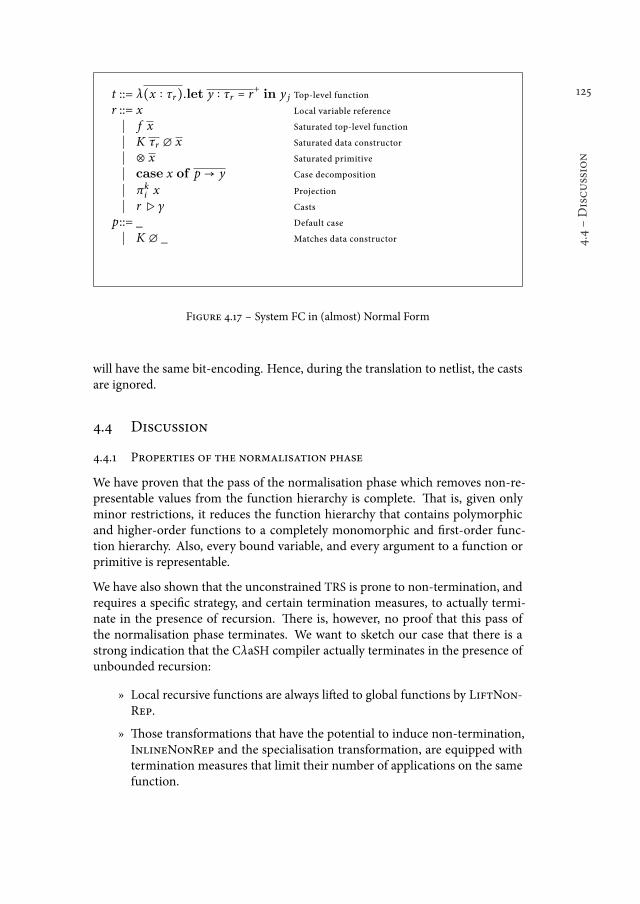
125

4.4śDiscussion

t ::= λ(x ∶ τr).let y ∶ τr ≙ r+in y j Top-level function

r ::= x Local variable reference

∣ f x Saturated top-level function

∣ K τr ∅ x Saturated data constructor

∣ ⊗ x Saturated primitive

∣ case x of p → y Case decomposition

∣ πki x Projection

∣ r▷ γ Casts

p::= _ Default case

∣ K ∅ _ Matches data constructor

Figure 4.17 ś System FC in (almost) Normal Form

will have the same bit-encoding. Hence, during the translation to netlist, the castsare ignored.

4.4 Discussion

4.4.1 Properties of the normalisation phase

We have proven that the pass of the normalisation phase which removes non-re-presentable values from the function hierarchy is complete. hat is, given onlyminor restrictions, it reduces the function hierarchy that contains polymorphicand higher-order functions to a completely monomorphic and irst-order func-tion hierarchy. Also, every bound variable, and every argument to a function orprimitive is representable.

We have also shown that the unconstrained TRS is prone to non-termination, andrequires a speciic strategy, and certain termination measures, to actually termi-nate in the presence of recursion. here is, however, no proof that this pass ofthe normalisation phase terminates. We want to sketch our case that there is astrong indication that the CλaSH compiler actually terminates in the presence ofunbounded recursion:

ż Local recursive functions are always lited to global functions by LiftNon-Rep.

ż hose transformations that have the potential to induce non-termination,InlineNonRep and the specialisation transformation, are equipped withtermination measures that limit their number of applications on the samefunction.

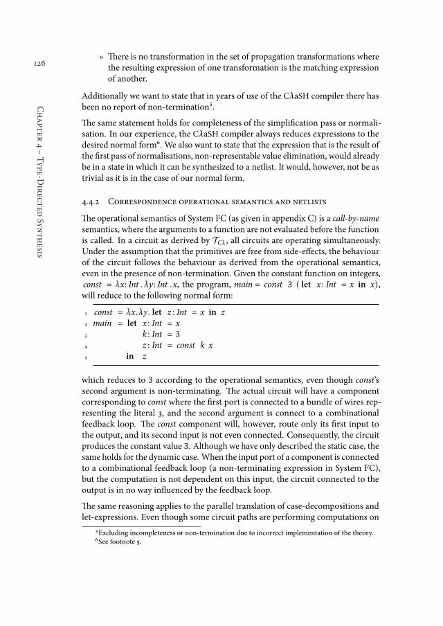
126

Chapter

4śType-D

irec

ted

Synthesis

ż here is no transformation in the set of propagation transformations wherethe resulting expression of one transformation is the matching expressionof another.

Additionally we want to state that in years of use of the CλaSH compiler there hasbeen no report of non-termination5.

he same statement holds for completeness of the simpliication pass or normali-sation. In our experience, the CλaSH compiler always reduces expressions to thedesired normal form6. We also want to state that the expression that is the result ofthe irst pass of normalisations, non-representable value elimination, would alreadybe in a state in which it can be synthesized to a netlist. It would, however, not be astrivial as it is in the case of our normal form.

4.4.2 Correspondence operational semantics and netlists

he operational semantics of System FC (as given in appendix C) is a call-by-namesemantics, where the arguments to a function are not evaluated before the functionis called. In a circuit as derived by TCλ , all circuits are operating simultaneously.Under the assumption that the primitives are free from side-efects, the behaviourof the circuit follows the behaviour as derived from the operational semantics,even in the presence of non-termination. Given the constant function on integers,const = λx: Int . λy: Int .x, the program, main = const 3 ( let x : Int = x in x),will reduce to the following normal form:

1 const = λx.λy. let z : Int = x in z2 main = let x : Int = x3 k : Int = 3

4 z : Int = const k x5 in z

which reduces to 3 according to the operational semantics, even though const’ssecond argument is non-terminating. he actual circuit will have a componentcorresponding to const where the irst port is connected to a bundle of wires rep-resenting the literal 3, and the second argument is connect to a combinationalfeedback loop. he const component will, however, route only its irst input tothe output, and its second input is not even connected. Consequently, the circuitproduces the constant value 3. Although we have only described the static case, thesame holds for the dynamic case. When the input port of a component is connectedto a combinational feedback loop (a non-terminating expression in System FC),but the computation is not dependent on this input, the circuit connected to theoutput is in no way inluenced by the feedback loop.

he same reasoning applies to the parallel translation of case-decompositions andlet-expressions. Even though some circuit paths are performing computations on

5Excluding incompleteness or non-termination due to incorrect implementation of the theory.6See footnote 5.

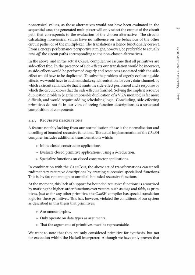
127

4.4.3śRec

ursivedescriptions

nonsensical values, as those alternatives would not have been evaluated in thesequential case, the generated multiplexer will only select the output of the circuitpath that corresponds to the evaluation of the chosen alternative. he circuitscalculating nonsensical values have no inluence on the behaviour of the othercircuit paths, or of the multiplexer. he translations is hence functionally correct.From a energy performance perspective it might, however, be preferable to actuallyturn of the circuit paths corresponding to the non-chosen alternatives.

In the above, and in the actual CλaSH compiler, we assume that all primitives areside-efect free. In the presence of side-efects our translation would be incorrect,as side-efects would be performed eagerly and resources associated with the side-efect would have to be duplicated. To solve the problem of eagerly evaluating side-efects, wewould have to add handshake synchronisation for every data-channel, bywhich a circuit can indicate that it wants the side-efect performed and a response bywhich the circuit knows that the side-efect is inished. Solving the implicit resourceduplication problem (e.g.the impossible duplication of a VGAmonitor) is far morediicult, and would require adding scheduling logic. Concluding, side-efectingprimitives do not it in our view of seeing function descriptions as a structuralcomposition of components.

4.4.3 Recursive descriptions

A feature notably lacking from our normalisation phase is the normalisation andunrolling of bounded recursive functions. he actual implementation of theCλaSHcompiler includes additional transformations which:

ż Inline closed constructor applications.

ż Evaluate closed primitive applications, using a δ-reduction.

ż Specialize functions on closed constructor applications.

In combination with the CaseCon, the above set of transformations can unrollrudimentary recursive descriptions by creating successive specialised functions.his is, by far, not enough to unroll all bounded recursive functions.

At the moment, this lack of support for bounded recursive functions is amortisedby marking the higher-order functions over vectors, such asmap and foldr, as prim-itives. Just as for any other primitive, the CλaSH compiler has special translationlogic for these primitives. his has, however, violated the conditions of our systemas described in this thesis that primitives:

ż Are monomorphic.

ż Only operate on data types as arguments.

ż hat the arguments of primitives must be representable.

We want to note that they are only considered primitive for synthesis, but notfor execution within the Haskell interpreter. Although we have only proven that

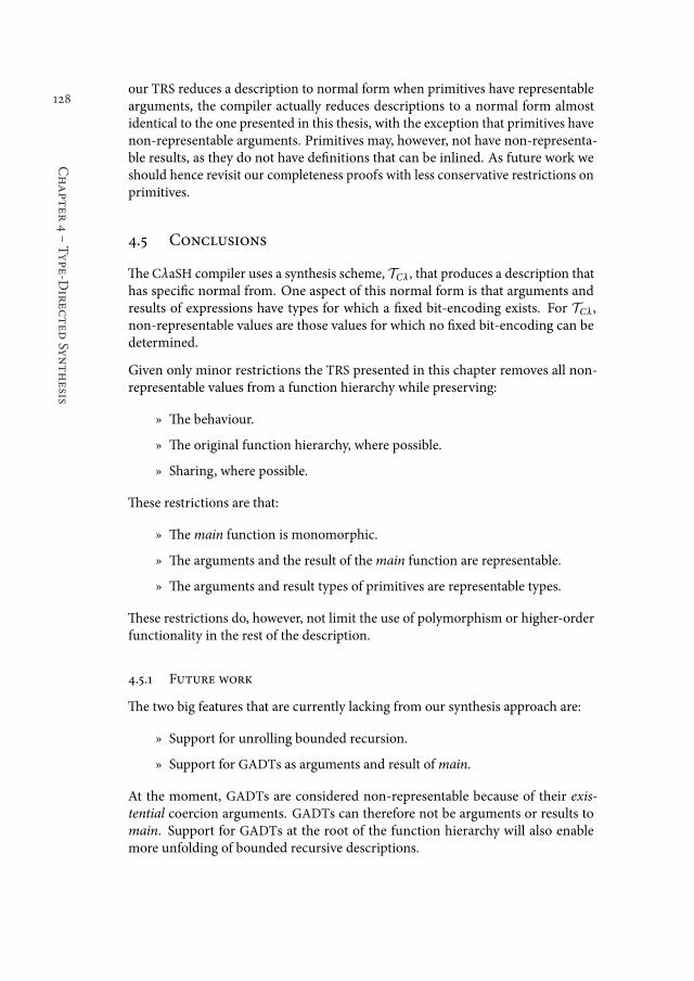
128

Chapter

4śType-D

irec

ted

Synthesis

our TRS reduces a description to normal form when primitives have representablearguments, the compiler actually reduces descriptions to a normal form almostidentical to the one presented in this thesis, with the exception that primitives havenon-representable arguments. Primitives may, however, not have non-representa-ble results, as they do not have deinitions that can be inlined. As future work weshould hence revisit our completeness proofs with less conservative restrictions onprimitives.

4.5 Conclusions

he CλaSH compiler uses a synthesis scheme, TCλ , that produces a description thathas speciic normal from. One aspect of this normal form is that arguments andresults of expressions have types for which a ixed bit-encoding exists. For TCλ ,non-representable values are those values for which no ixed bit-encoding can bedetermined.

Given only minor restrictions the TRS presented in this chapter removes all non-representable values from a function hierarchy while preserving:

ż he behaviour.

ż he original function hierarchy, where possible.

ż Sharing, where possible.

hese restrictions are that:

ż hemain function is monomorphic.

ż he arguments and the result of themain function are representable.

ż he arguments and result types of primitives are representable types.

hese restrictions do, however, not limit the use of polymorphism or higher-orderfunctionality in the rest of the description.

4.5.1 Future work

he two big features that are currently lacking from our synthesis approach are:

ż Support for unrolling bounded recursion.

ż Support for GADTs as arguments and result ofmain.

At the moment, GADTs are considered non-representable because of their exis-tential coercion arguments. GADTs can therefore not be arguments or results tomain. Support for GADTs at the root of the function hierarchy will also enablemore unfolding of bounded recursive descriptions.

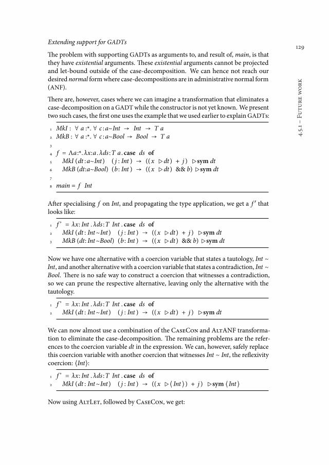
129

4.5.1śFuturework

Extending support for GADTs

he problem with supporting GADTs as arguments to, and result of,main, is thatthey have existential arguments. hese existential arguments cannot be projectedand let-bound outside of the case-decomposition. We can hence not reach ourdesired normal formwhere case-decompositions are in administrative normal form(ANF).

here are, however, cases where we can imagine a transformation that eliminates acase-decomposition on aGADTwhile the constructor is not yet known. We presenttwo such cases, the irst one uses the example that we used earlier to explainGADTs:

1 MkI : ∀ a :*. ∀ c :a~Int → Int → T a2 MkB : ∀ a :*. ∀ c :a~Bool → Bool → T a3

4 f = Λa :*.λx:a .λds :T a . case ds of5 MkI (dt :a~Int) ( j : Int ) → ((x ▷dt) + j ) ▷sym dt6 MkB (dt:a~Bool) (b : Int ) → ((x ▷dt) && b)▷sym dt7

8 main = f Int

Ater specialising f on Int, and propagating the type application, we get a f ′ thatlooks like:

1 f ’ = λx: Int . λds :T Int . case ds of2 MkI (dt : Int~Int ) ( j : Int ) → ((x ▷dt) + j ) ▷sym dt3 MkB (dt: Int~Bool) (b : Int ) → ((x ▷dt) && b)▷sym dt

Now we have one alternative with a coercion variable that states a tautology, Int ∼Int, and another alternativewith a coercion variable that states a contradiction, Int ∼Bool. here is no safe way to construct a coercion that witnesses a contradiction,so we can prune the respective alternative, leaving only the alternative with thetautology.

1 f ’ = λx: Int . λds :T Int . case ds of2 MkI (dt : Int~Int ) ( j : Int ) → ((x ▷dt) + j ) ▷sym dt

We can now almost use a combination of the CaseCon and AltANF transforma-tion to eliminate the case-decomposition. he remaining problems are the refer-ences to the coercion variable dt in the expression. We can, however, safely replacethis coercion variable with another coercion that witnesses Int ∼ Int, the relexivitycoercion: ⟨Int⟩:

1 f ’ = λx: Int . λds :T Int . case ds of2 MkI (dt : Int~Int ) ( j : Int ) → ((x ▷⟨ Int ⟩) + j ) ▷sym ⟨Int ⟩

Now using AltLet, followed by CaseCon, we get:

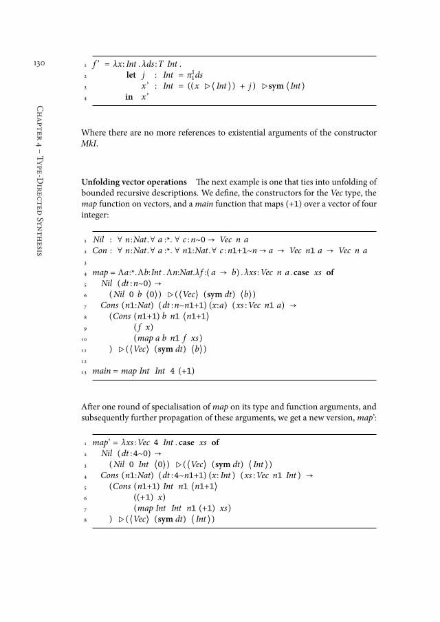
130

Chapter

4śType-D

irec

ted

Synthesis

1 f ’ = λx: Int . λds :T Int .2 let j : Int = π1

1ds3 x ’ : Int = ((x ▷⟨ Int ⟩) + j ) ▷sym ⟨Int ⟩4 in x ’

Where there are no more references to existential arguments of the constructorMkI.

Unfolding vector operations he next example is one that ties into unfolding ofbounded recursive descriptions. We deine, the constructors for the Vec type, themap function on vectors, and amain function that maps (+1) over a vector of fourinteger:

1 Nil : ∀ n :Nat.∀ a :*. ∀ c :n~0→ Vec n a2 Con : ∀ n :Nat.∀ a :*. ∀ n1:Nat.∀ c :n1+1~n→ a → Vec n1 a → Vec n a3

4 map = Λa:*.Λb:Int .Λn:Nat.λf :( a → b) . λxs :Vec n a . case xs of5 Nil (dt :n~0) →6 (Nil 0 b ⟨0⟩) ▷ (⟨Vec⟩ (sym dt) ⟨b⟩)7 Cons (n1:Nat) (dt :n~n1+1) (x:a) (xs :Vec n1 a) →8 (Cons (n1+1) b n1 ⟨n1+1⟩9 ( f x)

10 (map a b n1 f xs)11 ) ▷ (⟨Vec⟩ (sym dt) ⟨b⟩)12

13 main = map Int Int 4 (+1)

Ater one round of specialisation ofmap on its type and function arguments, andsubsequently further propagation of these arguments, we get a new version,map’:

1 map’ = λxs :Vec 4 Int . case xs of2 Nil (dt :4~0) →3 (Nil 0 Int ⟨0⟩) ▷ (⟨Vec⟩ (sym dt) ⟨ Int ⟩)4 Cons (n1:Nat) (dt :4~n1+1) (x: Int ) (xs :Vec n1 Int ) →5 (Cons (n1+1) Int n1 ⟨n1+1⟩6 ((+1) x)7 (map Int Int n1 (+1) xs)8 ) ▷ (⟨Vec⟩ (sym dt) ⟨ Int ⟩)

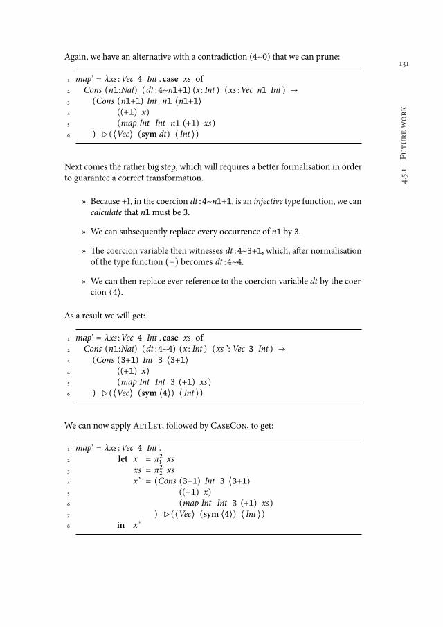
131

4.5.1śFuturework

Again, we have an alternative with a contradiction (4~0) that we can prune:

1 map’ = λxs :Vec 4 Int . case xs of2 Cons (n1:Nat) (dt :4~n1+1) (x: Int ) (xs :Vec n1 Int ) →3 (Cons (n1+1) Int n1 ⟨n1+1⟩4 ((+1) x)5 (map Int Int n1 (+1) xs)6 ) ▷ (⟨Vec⟩ (sym dt) ⟨ Int ⟩)

Next comes the rather big step, which will requires a better formalisation in orderto guarantee a correct transformation.

ż Because +1, in the coercion dt :4~n1+1, is an injective type function, we cancalculate that n1must be 3.

ż We can subsequently replace every occurrence of n1 by 3.

ż he coercion variable then witnesses dt :4~3+1, which, ater normalisationof the type function (+) becomes dt :4~4.

ż We can then replace ever reference to the coercion variable dt by the coer-cion ⟨4⟩.

As a result we will get:

1 map’ = λxs :Vec 4 Int . case xs of2 Cons (n1:Nat) (dt :4~4) (x : Int ) (xs ’: Vec 3 Int ) →3 (Cons (3+1) Int 3 ⟨3+1⟩4 ((+1) x)5 (map Int Int 3 (+1) xs)6 ) ▷ (⟨Vec⟩ (sym ⟨4⟩) ⟨ Int ⟩)

We can now apply AltLet, followed by CaseCon, to get:

1 map’ = λxs :Vec 4 Int .2 let x = π2

1 xs3 xs = π2

2 xs4 x ’ = (Cons (3+1) Int 3 ⟨3+1⟩5 ((+1) x)6 (map Int Int 3 (+1) xs)7 ) ▷ (⟨Vec⟩ (sym ⟨4⟩) ⟨ Int ⟩)8 in x ’

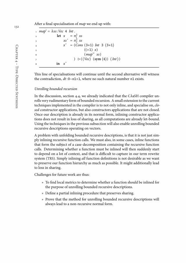
132

Chapter

4śType-D

irec

ted

Synthesis

Ater a inal specialisation ofmap we end up with:

1 map’ = λxs :Vec 4 Int .2 let x = π2

1 xs3 xs ’ = π2

2 xs4 x ’ = (Cons (3+1) Int 3 ⟨3+1⟩5 ((+1) x)6 (map’’ xs)7 ) ▷ (⟨Vec⟩ (sym ⟨4⟩) ⟨ Int ⟩)8 in x ’

his line of specialisations will continue until the second alternative will witnessthe contradiction, dt :0~n1+1, where no such natural number n1 exists.

Unrolling bounded recursion

In the discussion, section 4.4, we already indicated that the CλaSH compiler un-rolls very rudimentary form of bounded recursion. A small extension to the currenttechniques implemented in the compiler is to not only inline, and specialise on, clo-sed constructor applications, but also constructors applications that are not closed.Once our description is already in its normal form, inlining constructor applica-tions does not result in loss of sharing, as all computations are already let-bound.Using the techniques in the previous subsection will also enable unrolling boundedrecursive descriptions operating on vectors.

A problem with unfolding bounded recursive descriptions, is that it is not just sim-ply inlining recursive function calls. We must also, in some cases, inline functionsthat form the subject of a case-decomposition containing the recursive functioncalls. Determining whether a function must be inlined will then suddenly startto depend on a lot of context, and that is diicult to capture in our term rewritesystem (TRS). Simply inlining all function deinitions is not desirable as we wantto preserve our function hierarchy as much as possible. It might additionally leadto loss in sharing.

Challenges for future work are thus:

ż To ind local metrics to determine whether a function should be inlined forthe purpose of unrolling bounded recursive descriptions.

ż Deine a partial inlining procedure that preserves sharing.

ż Prove that the method for unrolling bounded recursive descriptions willalways lead to a non-recursive normal form.

133

134

135

5Advanced aspects of

circuit design in CλaSH

Abstract ś Even when descriptions use high-level abstractions, the CλaSHcompiler can synthesize eicient circuits. Case studies show that circuits de-signed in Haskell, and synthesized with the CλaSH compiler, are on par withhand-written VHDL, in both area and gate propagation delay. Even in the pres-ence of contemporary Haskell idioms and abstractions to write imperative code(for a control-oriented circuit) does the CλaSH compiler create results withdecent non-functional properties. To emphasize that our approach enablescorrect-by-construction descriptions, we demonstrate abstractions that allowus to automatically compose components that use back-pressure as their syn-chronisation method. Additionally, we show how cycle delays can be encodedin the type-signatures of components, allowing us to catch any synchronisationerror at compile-time.

5.1 Introduction

he previous two chapters introduced the ideas behind designing synchronouscircuits in Haskell, and synthesising these descriptions to a netlist. Chapter 3 in-troduced some small examples, but mainly to demonstrate the ideas behind thetechniques to design circuits. he CλaSH compiler has, however, been used formuch larger designs. It has been used to create various DSP circuits: such as il-ter banks [73], particle ilters [71][CB:11], spectral estimation techniques [36], amodel of the human cochlea [66], and stencil computations [72]. Additionally, theuse of higher-order functions to make correct-by-constructions trade-ofs betweena space/time unrolling of computations, and subsequent mapping to circuits, is

Parts of this chapter have been published in [CB:7] and [CB:9].

136

Chapter

5śAdva

nced

aspec

tsofcircuit

desig

nin

CλaSH

explored in [39, 70]. Finally, CλaSH has also been used to design a many-coreprocessor architecture that is based on data-low principles [48][CB:3].

here are hence many existing examples of using CλaSH for circuit design, andthe use of higher-order to make design trade-ofs. he purpose of this chapteris therefore not to give an overview how CλaSH can be used for circuit design ingeneral. Instead, it will focus on some of themore advanced aspects of circuit designin CλaSH.

As an introduction, the next section will describe the design of a medium sizedcircuit, a streaming reduction circuit [18], which is still designed in terms of ordi-nary function composition. Ater that, we move on to describing the larger CλaSHdemonstrator circuit, where we use two aspects that are novel in terms of synthesis-able circuit design in Haskell (compared to e.g. [26]): multiple clock domains, andthe use of monads to describe imperative, control-oriented, circuits. he last twosections will focus on the correct-by-construction composition of circuits, whereone section will use higher-order functions to compose circuits that use back-pres-sure, and the other section will use type-level functions and numbers to staticallyenforce correct synchronisation.

5.2 Streaming reduction circuit

When solving the matrix equation Ax ≙ b for a big sparse matrix A, one oten usesthe conjugate gradient algorithm [61]. A core operation of the conjugate gradientalgorithm is a sparse matrix-vector multiplication (SMxV), which we can performby taking the dot product for every row in the matrix. For an SMxV the number ofmultiplications and additions required for an elements in the result vector dependson the number of non-zeros in the respective row of the matrix. Working withloating pointer numbers, the multiplication and addition operations are otenpipelined in order to achieve reasonable operating frequencies.

In a pipelined arithmetic logic unit (ALU), a new operation can be scheduled everycycle, but it will take several cycles before the calculated result exits the pipeline. Wedemonstrate this behaviour in igure 5.1, where an addition is scheduled every cycle.For demonstrative purposes, in our notation the addition takes place immediately,and the result will then propagate through the pipeline.

As part of the dot product, we will have to sum all the numbers in a row of a matrix.Summing all elements in a row using a pipelined adder is, however, more complexthan it is when using a non-pipelined adder. Assume for instance that we want tosum three values in a row using a 14-stage pipelined adder. Adding the irst twovalues is trivial, ater that we will have to wait 14 cycles before the result of thisaddition can be added to the third value. While we wait, however, there may bevalues from other rows that also need to be summed. We hence desire to schedulethe pipeline so that it can reduce multiple rows simultaneously, of course, withoutaccidentally summing values from diferent rows.

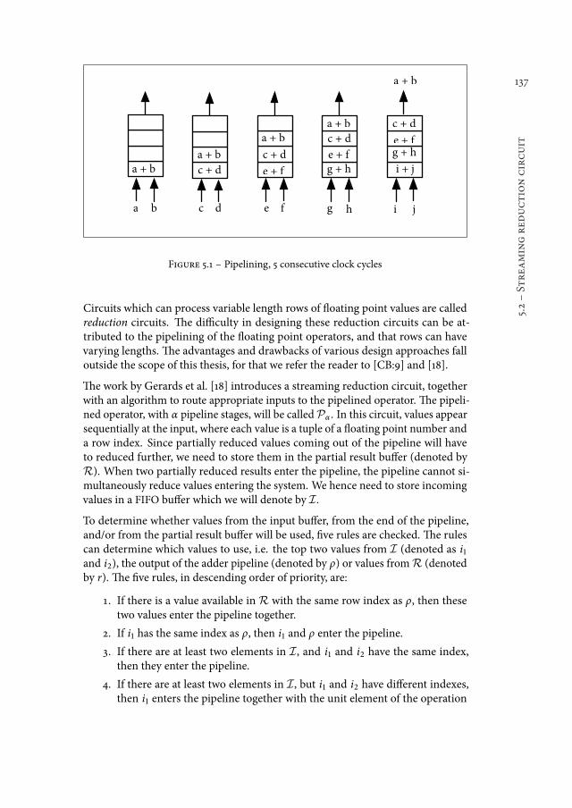
137

5.2śStrea

mingred

uctioncircuit

a + b

a + b

a + b

a + b

a + b

c + d

c + d

c + d

c + d

e + f

e + f

e + f

g + h

g + h

i + j

a b c d e f g h i j

Figure 5.1 ś Pipelining, 5 consecutive clock cycles

Circuits which can process variable length rows of loating point values are calledreduction circuits. he diiculty in designing these reduction circuits can be at-tributed to the pipelining of the loating point operators, and that rows can havevarying lengths. he advantages and drawbacks of various design approaches falloutside the scope of this thesis, for that we refer the reader to [CB:9] and [18].

he work by Gerards et al. [18] introduces a streaming reduction circuit, togetherwith an algorithm to route appropriate inputs to the pipelined operator. he pipeli-ned operator, with α pipeline stages, will be calledPα . In this circuit, values appearsequentially at the input, where each value is a tuple of a loating point number anda row index. Since partially reduced values coming out of the pipeline will haveto reduced further, we need to store them in the partial result bufer (denoted byR). When two partially reduced results enter the pipeline, the pipeline cannot si-multaneously reduce values entering the system. We hence need to store incomingvalues in a FIFO bufer which we will denote by I .

To determine whether values from the input bufer, from the end of the pipeline,and/or from the partial result bufer will be used, ive rules are checked. he rulescan determine which values to use, i.e. the top two values from I (denoted as i1and i2), the output of the adder pipeline (denoted by ρ) or values fromR (denotedby r). he ive rules, in descending order of priority, are:

1. If there is a value available inR with the same row index as ρ, then thesetwo values enter the pipeline together.

2. If i1 has the same index as ρ, then i1 and ρ enter the pipeline.

3. If there are at least two elements in I , and i1 and i2 have the same index,then they enter the pipeline.

4. If there are at least two elements in I , but i1 and i2 have diferent indexes,then i1 enters the pipeline together with the unit element of the operation

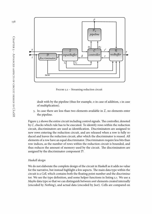
138

Chapter

5śAdva

nced

aspec

tsofcircuit

desig

nin

CλaSH

pipeline

controller resBu�erdiscriminator

inputBu�erdi

x

i� i�

δ

a� a�

ρ

r

r′

new

yD

I C

Pα

R

Figure 5.2 ś Streaming reduction circuit

dealt with by the pipeline (thus for example, 0 in case of addition, 1 in caseof multiplication).

5. In case there are less than two elements available in I , no elements enterthe pipeline.

Figure 5.2 shows the entire circuit including control signals. he controller, denotedby C, checks which rule has to be executed. To identify rows within the reductioncircuit, discriminators are used as identiication. Discriminators are assigned tonew rows entering the reduction circuit, and are released when a row is fully re-duced and leaves the reduction circuit, ater which the discriminator is reused. Allelements of a row have an equal discriminator. Discriminators require less bits thanrow indices, as the number of rows within the reduction circuit is bounded, andthus reduces the amount of memory used by the circuit. he discriminators areassigned by the discriminator componentD.

Haskell design

We do not elaborate the complete design of the circuit in Haskell as it adds no valuefor the narrative, but instead highlight a few aspects. hemain data type within thecircuit is a Cell, which contains both the loating point number and the discrimina-tor. We see the type deinition, and some helper functions in listing 5.1. We use aMaybe data type so that we can distinguish between unit elements created internally(encoded by Nothing), and actual data (encoded by Just). Cells are compared on

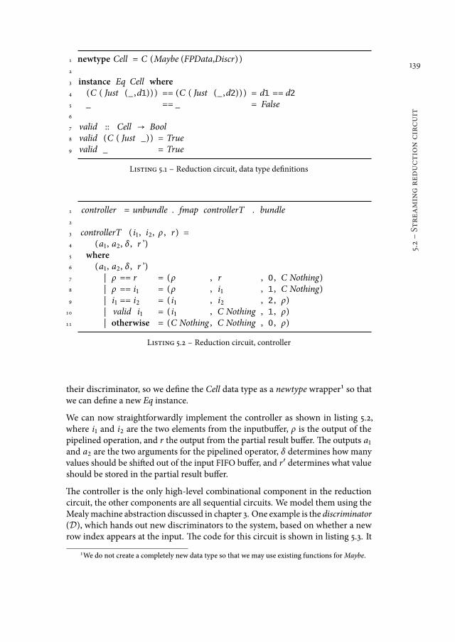
139

5.2śStrea

mingred

uctioncircuit

1 newtype Cell = C (Maybe (FPData,Discr) )2

3 instance Eq Cell where4 (C ( Just (_ ,d1))) == (C ( Just (_ ,d2))) = d1 == d25 _ == _ = False6

7 valid :: Cell → Bool8 valid (C ( Just _)) = True9 valid _ = True

Listing 5.1 ś Reduction circuit, data type deinitions

1 controller = unbundle . fmap controllerT . bundle2

3 controllerT ( i1 , i2, ρ , r) =4 (a1, a2, δ , r ’)5 where6 (a1, a2, δ , r ’)7 | ρ == r = (ρ , r , 0 , C Nothing)8 | ρ == i1 = (ρ , i1 , 1 , C Nothing)9 | i1 == i2 = ( i1 , i2 , 2 , ρ)

10 | valid i1 = ( i1 , C Nothing , 1 , ρ)11 | otherwise = (C Nothing , C Nothing , 0 , ρ)

Listing 5.2 ś Reduction circuit, controller

their discriminator, so we deine the Cell data type as a newtype wrapper¹ so thatwe can deine a new Eq instance.

We can now straightforwardly implement the controller as shown in listing 5.2,where i1 and i2 are the two elements from the inputbufer, ρ is the output of thepipelined operation, and r the output from the partial result bufer. he outputs a1and a2 are the two arguments for the pipelined operator, δ determines how manyvalues should be shited out of the input FIFO bufer, and r′ determines what valueshould be stored in the partial result bufer.

he controller is the only high-level combinational component in the reductioncircuit, the other components are all sequential circuits. We model them using theMealymachine abstraction discussed in chapter 3. One example is the discriminator(D), which hands out new discriminators to the system, based on whether a newrow index appears at the input. he code for this circuit is shown in listing 5.3. It

1We do not create a completely new data type so that we may use existing functions forMaybe.

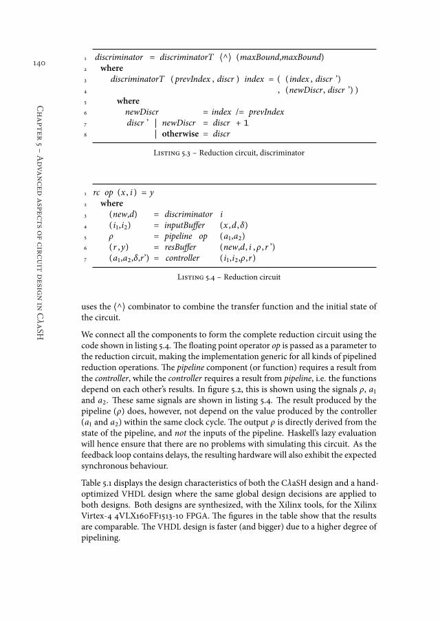
140

Chapter

5śAdva

nced

aspec

tsofcircuit

desig

nin

CλaSH

1 discriminator = discriminatorT ⟨^⟩ (maxBound,maxBound)2 where3 discriminatorT (prevIndex , discr ) index = ( ( index , discr ’)4 , (newDiscr , discr ’) )5 where6 newDiscr = index /= prevIndex7 discr ’ | newDiscr = discr + 1

8 | otherwise = discr

Listing 5.3 ś Reduction circuit, discriminator

1 rc op (x , i ) = y2 where3 (new,d) = discriminator i4 ( i1 ,i2) = inputBufer (x ,d ,δ)5 ρ = pipeline op (a1,a2)6 (r ,y) = resBufer (new,d , i ,ρ ,r ’)7 (a1,a2,δ,r’) = controller ( i1 ,i2,ρ,r)

Listing 5.4 ś Reduction circuit

uses the ⟨^⟩ combinator to combine the transfer function and the initial state ofthe circuit.

We connect all the components to form the complete reduction circuit using thecode shown in listing 5.4. he loating point operator op is passed as a parameter tothe reduction circuit, making the implementation generic for all kinds of pipelinedreduction operations. he pipeline component (or function) requires a result fromthe controller, while the controller requires a result from pipeline, i.e. the functionsdepend on each other’s results. In igure 5.2, this is shown using the signals ρ, a1and a2. hese same signals are shown in listing 5.4. he result produced by thepipeline (ρ) does, however, not depend on the value produced by the controller(a1 and a2) within the same clock cycle. he output ρ is directly derived from thestate of the pipeline, and not the inputs of the pipeline. Haskell’s lazy evaluationwill hence ensure that there are no problems with simulating this circuit. As thefeedback loop contains delays, the resulting hardware will also exhibit the expectedsynchronous behaviour.

Table 5.1 displays the design characteristics of both the CλaSH design and a hand-optimized VHDL design where the same global design decisions are applied toboth designs. Both designs are synthesized, with the Xilinx tools, for the XilinxVirtex-4 4VLX160FF1513-10 FPGA. he igures in the table show that the resultsare comparable. he VHDL design is faster (and bigger) due to a higher degree ofpipelining.

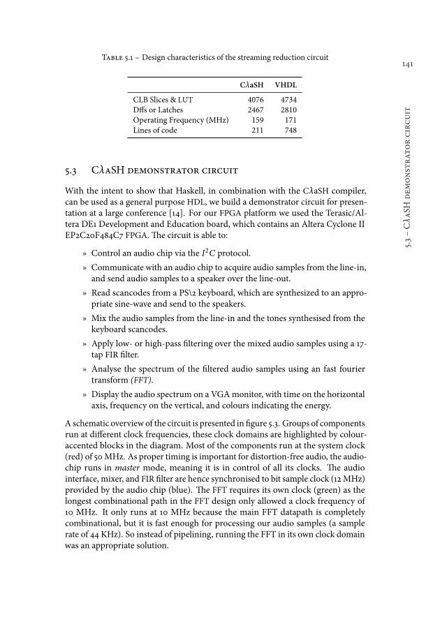
141

5.3śCλaSH

dem

onstrat

orcircuit

Table 5.1 ś Design characteristics of the streaming reduction circuit

CλaSH VHDL

CLB Slices & LUT 4076 4734Dfs or Latches 2467 2810Operating Frequency (MHz) 159 171Lines of code 211 748

5.3 CλaSH demonstrator circuit

With the intent to show that Haskell, in combination with the CλaSH compiler,can be used as a general purpose HDL, we build a demonstrator circuit for presen-tation at a large conference [14]. For our FPGA platform we used the Terasic/Al-tera DE1 Development and Education board, which contains an Altera Cyclone IIEP2C20F484C7 FPGA. he circuit is able to:

ż Control an audio chip via the I2C protocol.

ż Communicate with an audio chip to acquire audio samples from the line-in,and send audio samples to a speaker over the line-out.

ż Read scancodes from a PS\2 keyboard, which are synthesized to an appro-priate sine-wave and send to the speakers.

ż Mix the audio samples from the line-in and the tones synthesised from thekeyboard scancodes.

ż Apply low- or high-pass iltering over the mixed audio samples using a 17-tap FIR ilter.

ż Analyse the spectrum of the iltered audio samples using an fast fouriertransform (FFT).

ż Display the audio spectrum on a VGAmonitor, with time on the horizontalaxis, frequency on the vertical, and colours indicating the energy.

A schematic overview of the circuit is presented in igure 5.3. Groups of componentsrun at diferent clock frequencies, these clock domains are highlighted by colour-accented blocks in the diagram. Most of the components run at the system clock(red) of 50MHz. As proper timing is important for distortion-free audio, the audio-chip runs in master mode, meaning it is in control of all its clocks. he audiointerface, mixer, and FIR ilter are hence synchronised to bit sample clock (12MHz)provided by the audio chip (blue). he FFT requires its own clock (green) as thelongest combinational path in the FFT design only allowed a clock frequency of10 MHz. It only runs at 10 MHz because the main FFT datapath is completelycombinational, but it is fast enough for processing our audio samples (a samplerate of 44 KHz). So instead of pipelining, running the FFT in its own clock domainwas an appropriate solution.

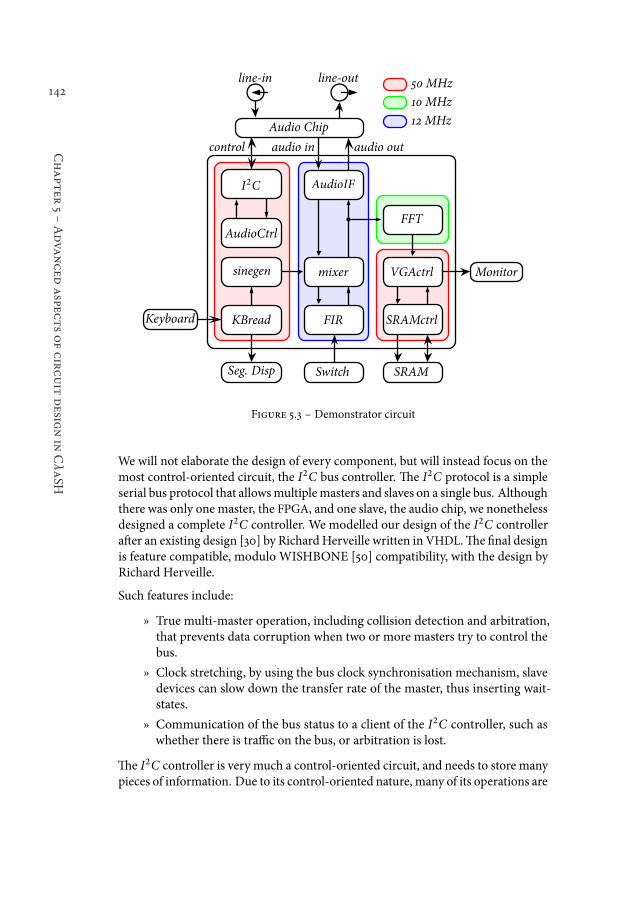
142

Chapter

5śAdva

nced

aspec

tsofcircuit

desig

nin

CλaSH

KBread

sinegen mixer

FIR

I�C AudioIF

VGActrl

AudioCtrl

FFT

SRAMctrl

Audio Chip

Monitor

Keyboard

SRAMSeg. Disp Switch

line-in line-out

control audio in audio out

�� MHz

�� MHz

�� MHz

Figure 5.3 ś Demonstrator circuit

We will not elaborate the design of every component, but will instead focus on themost control-oriented circuit, the I2C bus controller. he I2C protocol is a simpleserial bus protocol that allowsmultiplemasters and slaves on a single bus. Althoughthere was only one master, the FPGA, and one slave, the audio chip, we nonethelessdesigned a complete I2C controller. We modelled our design of the I2C controllerater an existing design [30] by RichardHerveille written inVHDL.he inal designis feature compatible, modulo WISHBONE [50] compatibility, with the design byRichard Herveille.

Such features include:

ż True multi-master operation, including collision detection and arbitration,that prevents data corruption when two or more masters try to control thebus.

ż Clock stretching, by using the bus clock synchronisation mechanism, slavedevices can slow down the transfer rate of the master, thus inserting wait-states.

ż Communication of the bus status to a client of the I2C controller, such aswhether there is traic on the bus, or arbitration is lost.

he I2C controller is very much a control-oriented circuit, and needs to store manypieces of information. Due to its control-oriented nature, many of its operations are

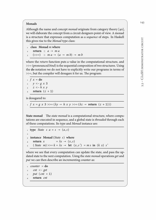
143

5.3śCλaSH

dem

onstrat

orcircuit

Monads

Although the name and conceptmonad originate from category theory [40],we will elaborate the concept from a circuit designers point of view. A monadis a structure that expresses computation as a sequence of steps. In Haskellthis gives rise to theMonad type class:

1 class Monadm where2 return :: a → m a3 (>>=) :: m a → (a → m b) → m b

where the return function puts a value in the computational structure, and>>= (pronounced bind) is the sequential composition of two structures. Usingthe do notation we do not have to explicitly write our programs in terms of>>=, but the compiler will desugare it for us. he program:

1 f x = do2 y <− g x 3

3 z <− h x y4 return (z + 1)

is desugared to:

1 f x = g x 3 >>= (λy → h x y >>= (λz → return (z + 1)) )

State monad he state monad is a computational structure, where compu-tations are executed in sequence, and a global state is threaded through eachof these computations. Its type andMonad instance are:

1 type State s a = s → (a , s )2

3 instance Monad (State s ) where4 return x = λs → (x , s )5 ( State m) >>= k = λs → let (x , s ’) = m s in (k x) s ’

where we see that every computation can update the state, and pass the up-dated state to the next computation. Using the state monad operations get andput we can then describe an incrementing counter as:

1 counter = do2 cnt <− get3 put ( cnt + 1)4 return cnt

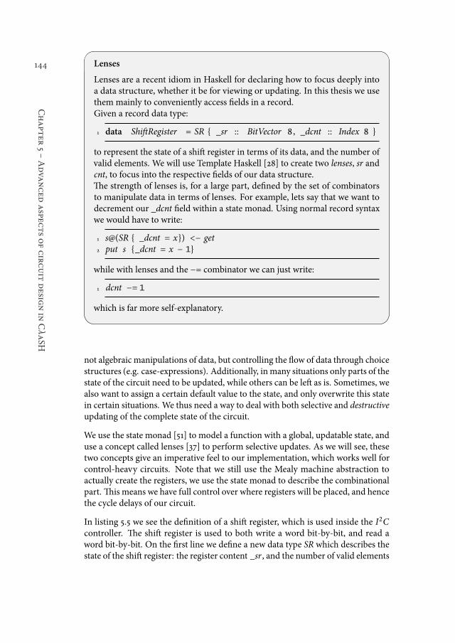
144

Chapter

5śAdva

nced

aspec

tsofcircuit

desig

nin

CλaSH

Lenses

Lenses are a recent idiom in Haskell for declaring how to focus deeply intoa data structure, whether it be for viewing or updating. In this thesis we usethem mainly to conveniently access ields in a record.Given a record data type:

1 data ShitRegister = SR { _sr :: BitVector 8 , _dcnt :: Index 8 }

to represent the state of a shit register in terms of its data, and the number ofvalid elements. We will use Template Haskell [28] to create two lenses, sr andcnt, to focus into the respective ields of our data structure.he strength of lenses is, for a large part, deined by the set of combinatorsto manipulate data in terms of lenses. For example, lets say that we want todecrement our _dcnt ield within a state monad. Using normal record syntaxwe would have to write:

1 s@(SR { _dcnt = x}) <− get2 put s {_dcnt = x − 1}

while with lenses and the −= combinator we can just write:

1 dcnt −= 1

which is far more self-explanatory.

not algebraic manipulations of data, but controlling the low of data through choicestructures (e.g. case-expressions). Additionally, inmany situations only parts of thestate of the circuit need to be updated, while others can be let as is. Sometimes, wealso want to assign a certain default value to the state, and only overwrite this statein certain situations. We thus need a way to deal with both selective and destructiveupdating of the complete state of the circuit.

We use the state monad [51] to model a function with a global, updatable state, anduse a concept called lenses [37] to perform selective updates. As we will see, thesetwo concepts give an imperative feel to our implementation, which works well forcontrol-heavy circuits. Note that we still use the Mealy machine abstraction toactually create the registers, we use the state monad to describe the combinationalpart. his means we have full control over where registers will be placed, and hencethe cycle delays of our circuit.

In listing 5.5 we see the deinition of a shit register, which is used inside the I2Ccontroller. he shit register is used to both write a word bit-by-bit, and read aword bit-by-bit. On the irst line we deine a new data type SR which describes thestate of the shit register: the register content _sr , and the number of valid elements

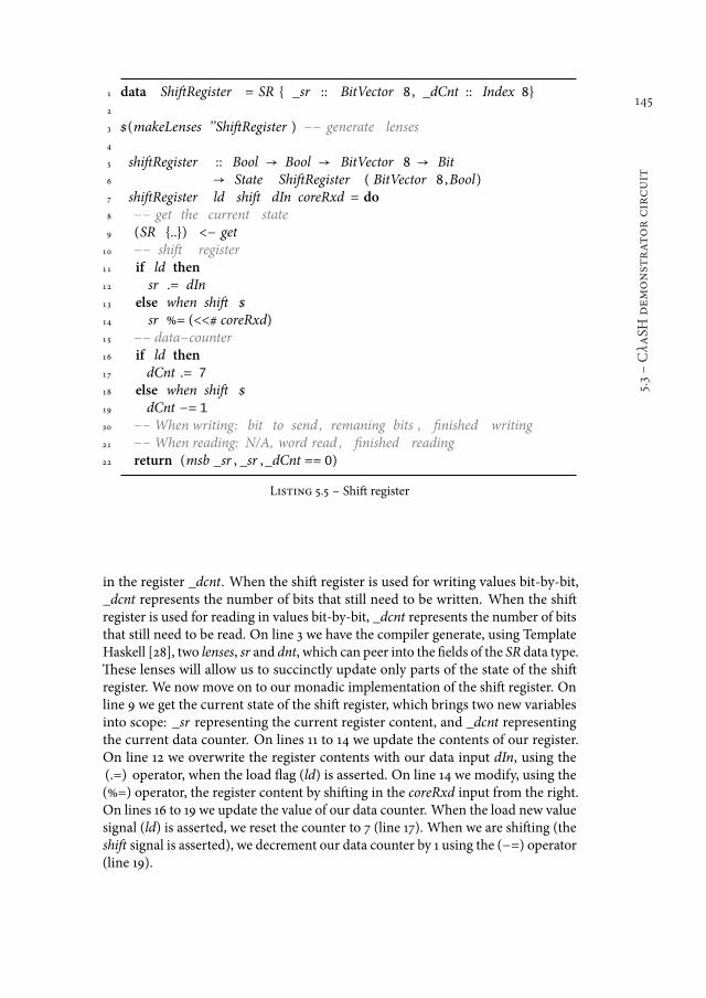
145

5.3śCλaSH

dem

onstrat

orcircuit

1 data ShitRegister = SR { _sr :: BitVector 8 , _dCnt :: Index 8}2

3 $(makeLenses ’’ShitRegister ) −− generate lenses4

5 shitRegister :: Bool → Bool → BitVector 8 → Bit6 → State ShitRegister ( BitVector 8 ,Bool)7 shitRegister ld shit dIn coreRxd = do8 −− get the current state9 (SR {..}) <− get

10 −− shit register11 if ld then12 sr .= dIn13 else when shit $14 sr %= (<<# coreRxd)15 −− data−counter16 if ld then17 dCnt .= 7

18 else when shit $19 dCnt −= 1

20 −−When writing: bit to send , remaning bits , inished writing21 −−When reading: N/A, word read , inished reading22 return (msb _sr , _sr ,_dCnt == 0)

Listing 5.5 ś Shit register

in the register _dcnt. When the shit register is used for writing values bit-by-bit,_dcnt represents the number of bits that still need to be written. When the shitregister is used for reading in values bit-by-bit, _dcnt represents the number of bitsthat still need to be read. On line 3 we have the compiler generate, using TemplateHaskell [28], two lenses, sr and dnt, which can peer into the ields of the SR data type.hese lenses will allow us to succinctly update only parts of the state of the shitregister. We now move on to our monadic implementation of the shit register. Online 9 we get the current state of the shit register, which brings two new variablesinto scope: _sr representing the current register content, and _dcnt representingthe current data counter. On lines 11 to 14 we update the contents of our register.On line 12 we overwrite the register contents with our data input dIn, using the(.=) operator, when the load lag (ld) is asserted. On line 14 we modify, using the(%=) operator, the register content by shiting in the coreRxd input from the right.On lines 16 to 19 we update the value of our data counter. When the load new valuesignal (ld) is asserted, we reset the counter to 7 (line 17). When we are shiting (theshit signal is asserted), we decrement our data counter by 1 using the (−=) operator(line 19).

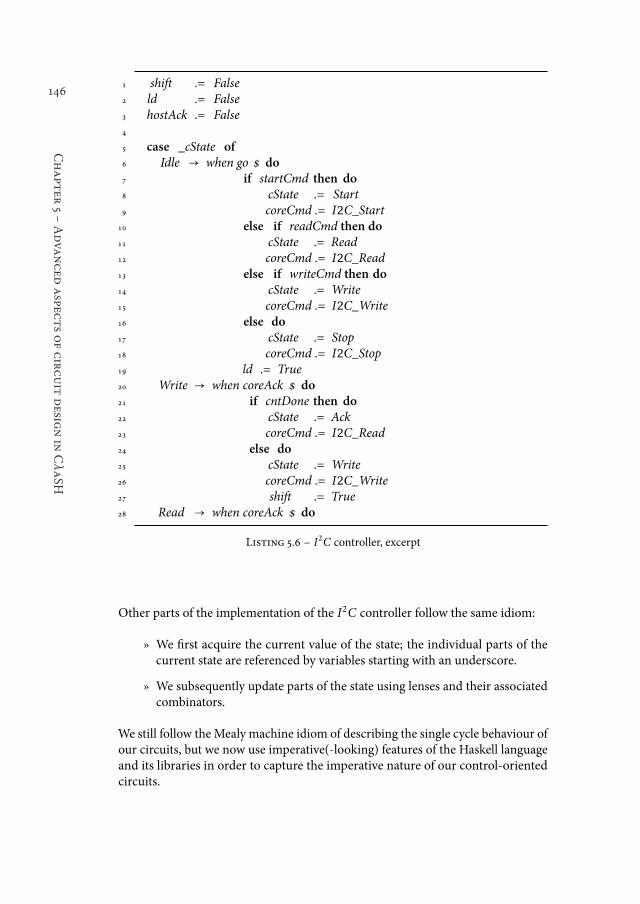
146

Chapter

5śAdva

nced

aspec

tsofcircuit

desig

nin

CλaSH

1 shit .= False2 ld .= False3 hostAck .= False4

5 case _cState of6 Idle → when go $ do7 if startCmd then do8 cState .= Start9 coreCmd .= I2C_Start

10 else if readCmd then do11 cState .= Read12 coreCmd .= I2C_Read13 else if writeCmd then do14 cState .= Write15 coreCmd .= I2C_Write16 else do17 cState .= Stop18 coreCmd .= I2C_Stop19 ld .= True20 Write → when coreAck $ do21 if cntDone then do22 cState .= Ack23 coreCmd .= I2C_Read24 else do25 cState .= Write26 coreCmd .= I2C_Write27 shit .= True28 Read → when coreAck $ do

Listing 5.6 ś I2C controller, excerpt

Other parts of the implementation of the I2C controller follow the same idiom:

ż We irst acquire the current value of the state; the individual parts of thecurrent state are referenced by variables starting with an underscore.

ż We subsequently update parts of the state using lenses and their associatedcombinators.

We still follow the Mealy machine idiom of describing the single cycle behaviour ofour circuits, but we now use imperative(-looking) features of the Haskell languageand its libraries in order to capture the imperative nature of our control-orientedcircuits.

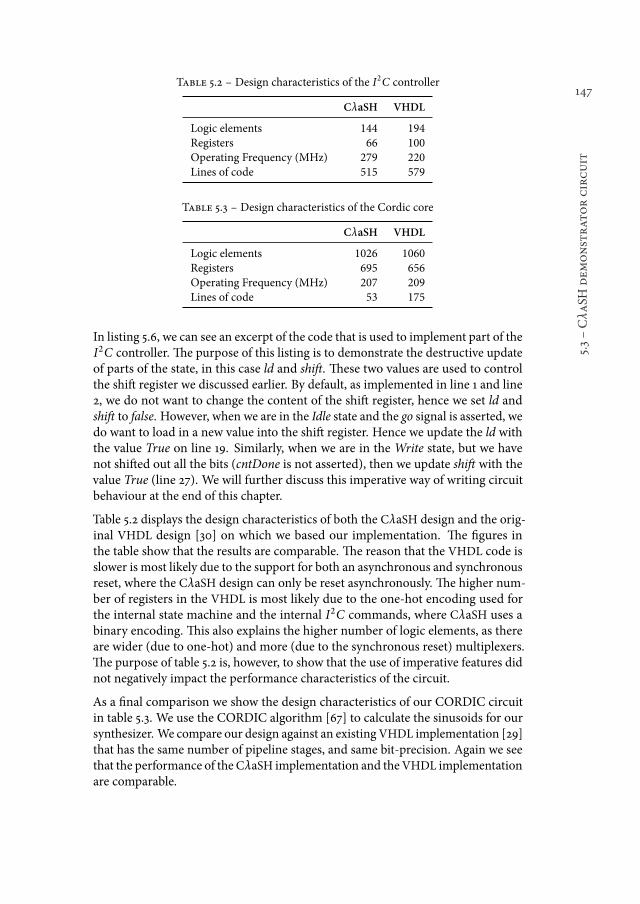
147

5.3śCλaSH

dem

onstrat

orcircuit

Table 5.2 ś Design characteristics of the I2C controller

CλaSH VHDL

Logic elements 144 194Registers 66 100Operating Frequency (MHz) 279 220Lines of code 515 579

Table 5.3 ś Design characteristics of the Cordic core

CλaSH VHDL

Logic elements 1026 1060Registers 695 656Operating Frequency (MHz) 207 209Lines of code 53 175

In listing 5.6,we can see an excerpt of the code that is used to implement part of theI2C controller. he purpose of this listing is to demonstrate the destructive updateof parts of the state, in this case ld and shit. hese two values are used to controlthe shit register we discussed earlier. By default, as implemented in line 1 and line2, we do not want to change the content of the shit register, hence we set ld andshit to false. However, when we are in the Idle state and the go signal is asserted, wedo want to load in a new value into the shit register. Hence we update the ld withthe value True on line 19. Similarly, when we are in theWrite state, but we havenot shited out all the bits (cntDone is not asserted), then we update shit with thevalue True (line 27). We will further discuss this imperative way of writing circuitbehaviour at the end of this chapter.

Table 5.2 displays the design characteristics of both the CλaSH design and the orig-inal VHDL design [30] on which we based our implementation. he igures inthe table show that the results are comparable. he reason that the VHDL code isslower is most likely due to the support for both an asynchronous and synchronousreset, where the CλaSH design can only be reset asynchronously. he higher num-ber of registers in the VHDL is most likely due to the one-hot encoding used forthe internal state machine and the internal I2C commands, where CλaSH uses abinary encoding. his also explains the higher number of logic elements, as thereare wider (due to one-hot) and more (due to the synchronous reset) multiplexers.he purpose of table 5.2 is, however, to show that the use of imperative features didnot negatively impact the performance characteristics of the circuit.

As a inal comparison we show the design characteristics of our CORDIC circuitin table 5.3. We use the CORDIC algorithm [67] to calculate the sinusoids for oursynthesizer. We compare our design against an existingVHDL implementation [29]that has the same number of pipeline stages, and same bit-precision. Again we seethat the performance of theCλaSH implementation and theVHDL implementationare comparable.

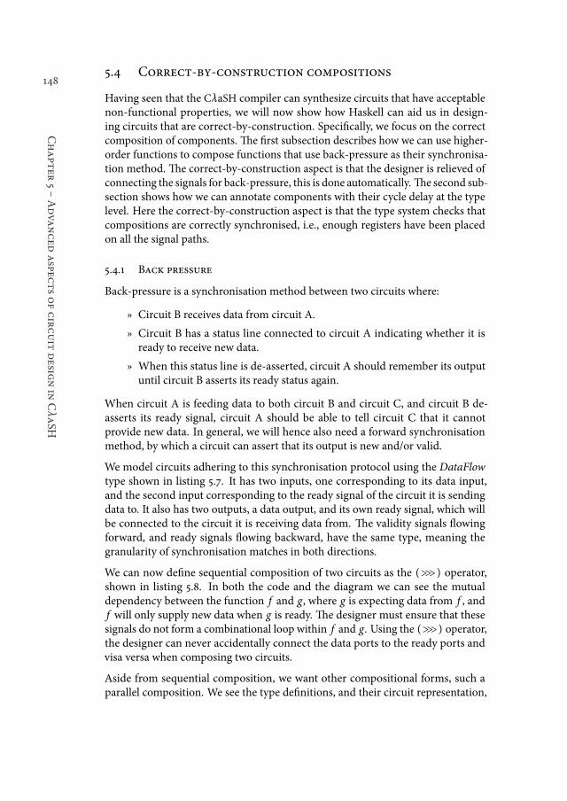
148

Chapter

5śAdva

nced

aspec

tsofcircuit

desig

nin

CλaSH

5.4 Correct-by-construction compositions

Having seen that the CλaSH compiler can synthesize circuits that have acceptablenon-functional properties, we will now show how Haskell can aid us in design-ing circuits that are correct-by-construction. Speciically, we focus on the correctcomposition of components. he irst subsection describes how we can use higher-order functions to compose functions that use back-pressure as their synchronisa-tion method. he correct-by-construction aspect is that the designer is relieved ofconnecting the signals for back-pressure, this is done automatically. he second sub-section shows how we can annotate components with their cycle delay at the typelevel. Here the correct-by-construction aspect is that the type system checks thatcompositions are correctly synchronised, i.e., enough registers have been placedon all the signal paths.

5.4.1 Back pressure

Back-pressure is a synchronisation method between two circuits where:

ż Circuit B receives data from circuit A.

ż Circuit B has a status line connected to circuit A indicating whether it isready to receive new data.

ż When this status line is de-asserted, circuit A should remember its outputuntil circuit B asserts its ready status again.

When circuit A is feeding data to both circuit B and circuit C, and circuit B de-asserts its ready signal, circuit A should be able to tell circuit C that it cannotprovide new data. In general, we will hence also need a forward synchronisationmethod, by which a circuit can assert that its output is new and/or valid.

We model circuits adhering to this synchronisation protocol using the DataFlowtype shown in listing 5.7. It has two inputs, one corresponding to its data input,and the second input corresponding to the ready signal of the circuit it is sendingdata to. It also has two outputs, a data output, and its own ready signal, which willbe connected to the circuit it is receiving data from. he validity signals lowingforward, and ready signals lowing backward, have the same type, meaning thegranularity of synchronisation matches in both directions.

We can now deine sequential composition of two circuits as the (⋙) operator,shown in listing 5.8. In both the code and the diagram we can see the mutualdependency between the function f and g, where g is expecting data from f , andf will only supply new data when g is ready. he designer must ensure that thesesignals do not form a combinational loop within f and g. Using the (⋙) operator,the designer can never accidentally connect the data ports to the ready ports andvisa versa when composing two circuits.

Aside from sequential composition, we want other compositional forms, such aparallel composition. We see the type deinitions, and their circuit representation,

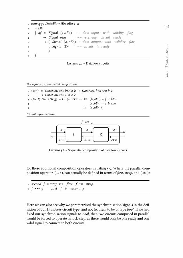
149

5.4.1śBackpressure

1 newtype DataFlow iEn oEn i o2 = DF3 { df :: Signal ( i , iEn) −− data input , with validity lag4 → Signal oEn −− receiving circuit ready5 → ( Signal (o ,oEn) −− data output , with validity lag6 , Signal iEn −− circuit is ready7 )8 }

Listing 5.7 ś Datalow circuits

Back-pressure, sequential composition

1 (⋙) :: DataFlow aEn bEn a b → DataFlow bEn cEn b c2 → DataFlow aEn cEn a c3 (DF f) ⋙ (DF g) = DF (λa cEn → let (b ,aEn) = f a bEn4 (c ,bEn) = g b cEn5 in (c ,aEn))

Circuit representation

f � g

fa b c

aEn bEn cEn

g

Listing 5.8 ś Sequential composition of datalow circuits

for these additional composition operators in listing 5.9. Where the parallel com-position operator, (⋆⋆⋆), can actually be deined in terms of irst, swap, and (⋙):

1 second f = swap⋙ irst f ⋙ swap2 f ⋆⋆⋆ g = irst f ⋙ second g

Here we can also see why we parametrised the synchronisation signals in the dei-nition of our DataFlow circuit type, and not ix them to be of type Bool. If we hadixed our synchronisation signals to Bool, then two circuits composed in parallelwould be forced to operate in lock-step, as there would only be one ready and onevalid signal to connect to both circuits.

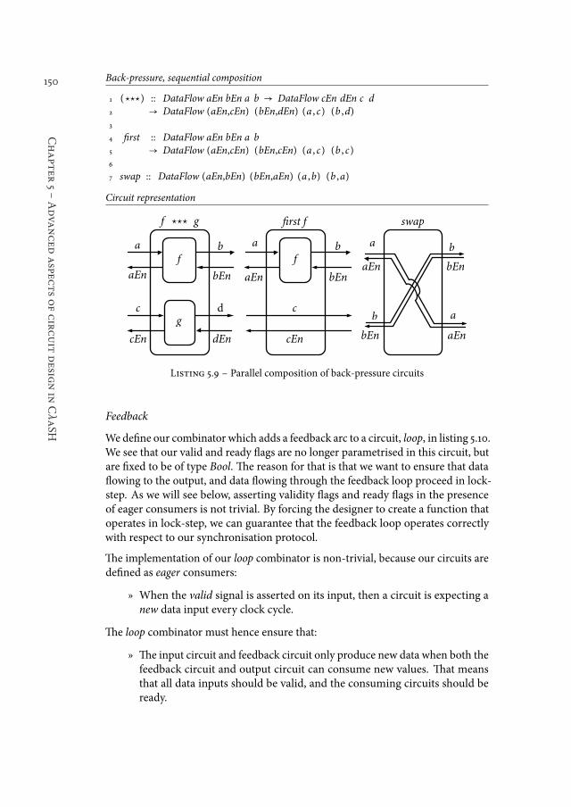
150

Chapter

5śAdva

nced

aspec

tsofcircuit

desig

nin

CλaSH

Back-pressure, sequential composition

1 (⋆⋆⋆) :: DataFlow aEn bEn a b → DataFlow cEn dEn c d2 → DataFlow (aEn,cEn) (bEn,dEn) (a , c) (b ,d)3

4 irst :: DataFlow aEn bEn a b5 → DataFlow (aEn,cEn) (bEn,cEn) (a , c) (b , c)6

7 swap :: DataFlow (aEn,bEn) (bEn,aEn) (a ,b) (b ,a)

Circuit representation

f ��� g

fa b

c

aEn bEn

cEn

gd

dEn

f

a b

aEn bEn

�rst f

c

cEn

ab

aEn bEn

b

bEn

a

aEn

swap

Listing 5.9 ś Parallel composition of back-pressure circuits

Feedback

Wedeine our combinator which adds a feedback arc to a circuit, loop, in listing 5.10.We see that our valid and ready lags are no longer parametrised in this circuit, butare ixed to be of type Bool. he reason for that is that we want to ensure that datalowing to the output, and data lowing through the feedback loop proceed in lock-step. As we will see below, asserting validity lags and ready lags in the presenceof eager consumers is not trivial. By forcing the designer to create a function thatoperates in lock-step, we can guarantee that the feedback loop operates correctlywith respect to our synchronisation protocol.

he implementation of our loop combinator is non-trivial, because our circuits aredeined as eager consumers:

ż When the valid signal is asserted on its input, then a circuit is expecting anew data input every clock cycle.

he loop combinator must hence ensure that:

ż he input circuit and feedback circuit only produce new data when both thefeedback circuit and output circuit can consume new values. hat meansthat all data inputs should be valid, and the consuming circuits should beready.

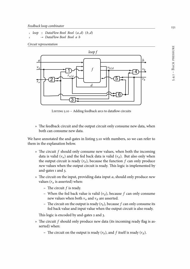
151

5.4.1śBackpressure

Feedback loop combinator

1 loop :: DataFlow Bool Bool (a ,d) (b ,d)2 → DataFlow Bool Bool a b

Circuit representation

f

a b

rarb

d

loop f

1va

vbvb�d

ra�d

2

6

5

4

3

Listing 5.10 ś Adding feedback arcs to datalow circuits

ż he feedback circuit and the output circuit only consume new data, whenboth can consume new data.

We have annotated the and-gates in listing 5.10 with numbers, so we can refer tothem in the explanation below.

ż he circuit f should only consume new values, when both the incomingdata is valid (va) and the fed back data is valid (vd ). But also only whenthe output circuit is ready (rb), because the function f can only producenew values when the output circuit is ready. his logic is implemented byand-gates 1 and 3.

ż he circuit on the input, providing data input a, should only produce newvalues (ra is asserted) when:

ś he circuit f is ready.

ś When the fed back value is valid (vd ), because f can only consumenew values when both va and vd are asserted.

ś he circuit on the output is ready (rb), because f can only consume itsfed back value and input value when the output circuit is also ready.

his logic is encoded by and-gates 2 and 3.

ż he circuit f should only produce new data (its incoming ready lag is as-serted) when:

ś he circuit on the output is ready (rb), and f itself is ready (rd ).

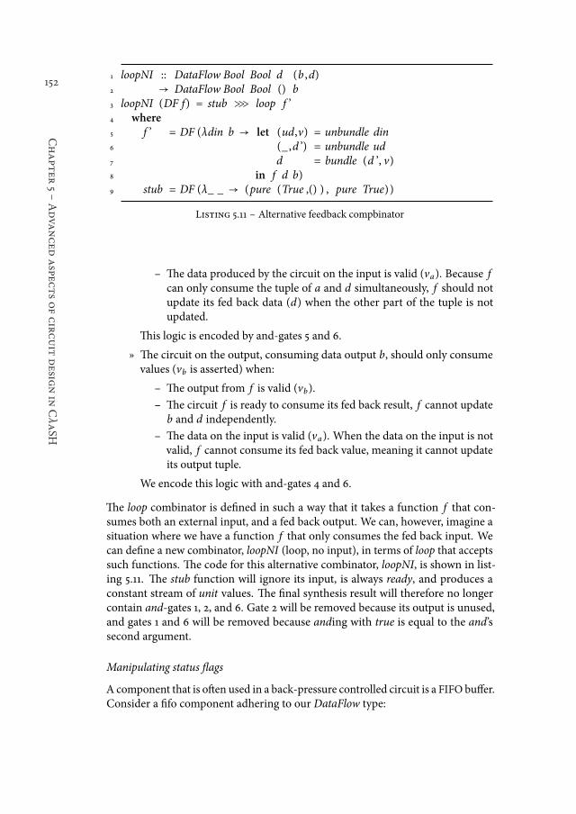
152

Chapter

5śAdva

nced

aspec

tsofcircuit

desig

nin

CλaSH

1 loopNI :: DataFlow Bool Bool d (b ,d)2 → DataFlow Bool Bool () b3 loopNI (DF f) = stub ⋙ loop f ’4 where5 f ’ = DF (λdin b → let (ud,v) = unbundle din6 (_ ,d ’) = unbundle ud7 d = bundle (d ’, v)8 in f d b)9 stub = DF (λ_ _ → (pure (True ,() ) , pure True))

Listing 5.11 ś Alternative feedback compbinator

ś he data produced by the circuit on the input is valid (va). Because fcan only consume the tuple of a and d simultaneously, f should notupdate its fed back data (d) when the other part of the tuple is notupdated.

his logic is encoded by and-gates 5 and 6.

ż he circuit on the output, consuming data output b, should only consumevalues (vb is asserted) when:

ś he output from f is valid (vb).

ś he circuit f is ready to consume its fed back result, f cannot updateb and d independently.

ś he data on the input is valid (va). When the data on the input is notvalid, f cannot consume its fed back value, meaning it cannot updateits output tuple.

We encode this logic with and-gates 4 and 6.

he loop combinator is deined in such a way that it takes a function f that con-sumes both an external input, and a fed back output. We can, however, imagine asituation where we have a function f that only consumes the fed back input. Wecan deine a new combinator, loopNI (loop, no input), in terms of loop that acceptssuch functions. he code for this alternative combinator, loopNI, is shown in list-ing 5.11. he stub function will ignore its input, is always ready, and produces aconstant stream of unit values. he inal synthesis result will therefore no longercontain and-gates 1, 2, and 6. Gate 2 will be removed because its output is unused,and gates 1 and 6 will be removed because anding with true is equal to the and’ssecond argument.

Manipulating status lags

A component that is oten used in a back-pressure controlled circuit is a FIFO bufer.Consider a ifo component adhering to our DataFlow type:

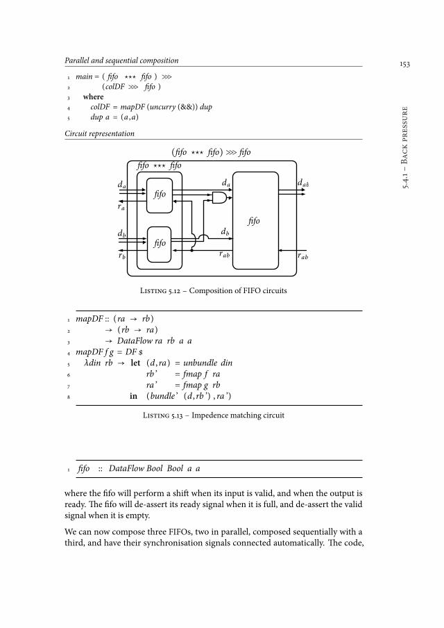
153

5.4.1śBackpressure

Parallel and sequential composition

1 main = ( ifo ⋆⋆⋆ ifo ) ⋙2 (colDF ⋙ ifo )3 where

4 colDF = mapDF (uncurry (&&)) dup5 dup a = (a ,a)

Circuit representation

�fo ��� �fo

�fo

�fo

�fo

(�fo ��� �fo)� �fo

da

ra

db

rb rab

dab

rab

db

da

Listing 5.12 ś Composition of FIFO circuits

1 mapDF :: (ra → rb)2 → (rb → ra)3 → DataFlow ra rb a a4 mapDF f g = DF $5 λdin rb → let (d , ra) = unbundle din6 rb ’ = fmap f ra7 ra ’ = fmap g rb8 in (bundle ’ (d , rb ’) , ra ’)

Listing 5.13 ś Impedence matching circuit

1 ifo :: DataFlow Bool Bool a a

where the ifo will perform a shit when its input is valid, and when the output isready. he ifo will de-assert its ready signal when it is full, and de-assert the validsignal when it is empty.

We can now compose three FIFOs, two in parallel, composed sequentially with athird, and have their synchronisation signals connected automatically. he code,

154

Chapter

5śAdva

nced

aspec

tsofcircuit

desig

nin

CλaSH

1 newtype DSignal ( delay :: Nat) a = D { toSignal :: Signal a }2 deriving (Functor , Applicative ,Num)

Listing 5.14 ś Delay annotated signals

and corresponding circuit interpretation can be seen in listing 5.12. Here we seethat we need an additional function,mapDF. he reason for that is that we need tocorrectly match the status signals of two FIFOs in parallel with the third FIFO. heparallel composition is expecting two ready lags to low backwards, and is oferingtwo valid lags in the forward direction. he third FIFO is, however, only oferingone ready lag, and expecting only one valid lag. Our inal combinator, mapDF(listing 5.13), can thus performs arbitrary manipulation on the status lags, in orderfor the connections such as the above to match up.

hemapDF function is also useful when specifying feedback loops. For example,we can build a derivative of our loop combinator, one that always adds a FIFO buferon the feedback edge:

1 loopFIFO :: DataFlow Bool Bool (a ,d) (b ,d)2 → DataFlow Bool Bool a b3 loopFIFO f = loop ( f ⋙ dupDF⋙ second ifo ⋙ colDF)4 where5 dupDF =mapDF dup (uncurry (&&))6 colDF = mapDF (uncorry (&&)) dup7 dup a = (a ,a)

where dubDF duplicates the valid signals lowing forward, and logically and’s theready signals lowing backwards. he colDF operates in the opposite direction,merging the valid signals, and duplicating the ready signals.

5.4.2 Delay annotations

he datalow method described in the previous section is one approach to makecircuit self-synchronising. Such a self-synchronising approach is oten used whencycle delays of computations are not ixed, i.e., when iteratively calculating a valueuntil it has a desired property. In other cases, however, diferent paths througha circuit accumulate distinct delays. When these paths are merged through anoperation, it is oten desired that these path are synchronised, that is, that bothpaths have accumulated the same number of delay. In this section we describehow signals can be annotated with their accumulated delay in their type, and howcomposition of functions are only type-correct when the function arguments havethe expected amount of accumulated delay.

he data type deinition of our annotated signal type is given in listing 5.14. hedelay annotation is a phantom type, just as the length annotation on our Vector

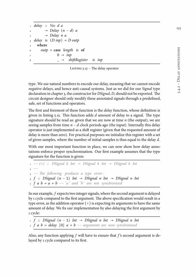
155

5.4.2śDelay

annotations

1 delay :: Vec d a2 → Delay (n − d) a3 → Delay n a4 delay is (D inp) = D outp5 where6 outp = case length is of7 0 → inp8 _ → shitRegister is inp

Listing 5.15 ś he delay operator

type. We use natural numbers to encode our delay, meaning that we cannot encodenegative delays, and hence anti-causal systems. Just as we did for our Signal typedeclaration in chapter 3, the constructor forDSignal,D, should not be exported. hecircuit designer should only modify these annotated signals through a predeined,safe, set of functions and operators.

he irst and foremost of these function is the delay function, whose deinition isgiven in listing 5.15. his function adds d amount of delay to a signal. he typesignature should be read as: given that we are now at time n (the output), we areseeing samples from time n − d clock periods ago (the input). Internally this delayoperator is just implemented as a shit register (given that the requested amount ofdelay is more than zero). For practical purposes we initialize this register with a setof given samples, where the number of initial samples is thus equal to the delay d.

With our most important function in place, we can now show how delay anno-tations enforce proper synchronisation. Our irst example assumes that the typesignature for the function is given:

1 −− (+) :: DSignal k Int → DSignal k Int → DSignal k Int2 −−3 −−he following produces a type error :4 f :: DSignal (n − 1) Int → DSignal n Int → DSignal n Int5 f a b = a + b −− ’a ’ and ’b ’ are not synchronised

In our example, f expects two integer signals, where the second argument is delayedby 1 cycle compared to the irst argument. he above speciication would result in atype error, as the addition operator (+) is expecting its arguments to have the sameamount of delay. We ix our implementation by also delaying the irst argument by1 cycle:

1 f :: DSignal (n − 1) Int → DSignal n Int → DSignal n Int2 f a b = delay [0] a + b −− arguments are now synchronised

Also, any function applying f will have to ensure that f ’s second argument is de-layed by 1 cycle compared to its irst.

156

Chapter

5śAdva

nced

aspec

tsofcircuit

desig

nin

CλaSH

1 unsafeFromSignal :: Proxy n → Signal a → DSignal n a2 unsafeFromSignal _ s = D s

Listing 5.16 ś Unsafe delay annotation

Conversion to Signal

As explained earlier, the constructor forDSignal,D, will not be exported, so that thecircuit designer cannot subvert its invariants by accident. Of course, it is imperativethat the designer can place a circuit deined in terms of DSignal, in a larger, lessrestricted, circuit deined in terms of Signal. he most straightforward operation isstripping the signal from its delay information:

1 toSignal :: DSignal n a → Signal a

which is just the ield extractor deined as part of our newtype deinition ofDSignal.

Dropping delay information is always safe, in terms of the invariants implied by thetype ofDSignal. Adding delay information requiresmore careful consideration. hesafest way to add a delay annotation on a normal signal is to add a delay annotationof zero cycles:

1 fromSignal :: Signal a → DSignal 0 a2 fromSignal s = D s

his new function will allow a designer to coerce any DSignal to have zero delay byusing: ( fromSignal . toSignal ) :: DSignal n a → DSignal 0 a. However, aslong aswe annotate functionswith polymorphic delay values, the risks of subvertingthe invariants of DSignal are reduced.

Let us assume that a circuit designer wants to use our circuit deined earlier, f ,within the function g, where g which is deined in terms of Signals. Having onlythe fromSignal function available, the second argument of g will have to be explicitlydelayed when applied to f :

1 g :: Signal Int → Signal Int → Signal Int2 g a b = toSignal ( f ( fromSignal a) ( delay [0] ( fromSignal b)) )

However, it might be the case that the designer knows that g’s second argumentis actually already delayed by one clock cycle compared to g’s irst argument. Inthat case, adding an extra delay to the second argument of f will actually cause thearguments of f to be improperly synchronised.

We hence need a third conversion function, given in listing 5.16, that allows thedesigner to explicitly annotate a signal with its delay. We preix the function with

157

5.4.2śDelay

annotations

the word, unsafe, to indicate to the designer that this function has to potential tosubvert invariants of DSignal. Because there is a strict phase distinction betweentypes and terms, we cannot make a function of the type unsafeFromSignal :: n →Signal a → DSignal n a, where nwould be both a type and a term. We therefore

use the Proxy data type, which, as the name suggests, acts like a term-level proxyfor the type n. Going back to our example, we can now write g as:

1 g :: Signal Int → Signal Int → Signal Int2 g a b = toSignal ( f ( fromSignal a)3 (unsafeFromSignal (Proxy :: Proxy 1) b))

Unlike the fromSignal function, unsafeFromSignal is able to completely subvert theinvariants of DSignal. hat is, we can redeine f , erroneously, but type-correct, as:

1 f :: DSignal (n−1) Int → DSignal n Int → DSignal n Int2 f a b = (( unsafeFromSignal (Proxy :: Proxy n) . toSignal ) a) + b

he unsafeFromSignal function is hence a truly unsafe operation. Both fromSig-nal and unsafeFromSignal are, however, needed in order to interact with circuitspeciications that are not annotated with delays.

Feedback

With delays encoded in the types, we can no longer deine feedback using standardvalue recursion. For example, using normal Signals, we can describe aMAC circuit:

1 mac x y = acc ’2 where3 acc ’ = (x * y) + acc4 acc = register 0 acc ’

where value recursion is used to model the feedback loop. However, when we tryto the same using DSignal and the delay function:

1 mac x y = acc ’2 where3 acc ’ = (x * y) + acc4 acc = delay [0] acc ’

we get a type error² because delay is expecting acc’ to be of type, DSignal (n−1) a,however, acc’ is deined in terms of acc, which is of type, DSignal n a. Actually,the only type-correct feedback loops that we can specify with the operators that wehave seen until now, are the unsound combinational feedback loops.

2Actually, in the polymorphic setting we get a function with an insoluble constraint, n ~ n − 1,which we cannot solve once we move to a monomorphic setting.

158

Chapter

5śAdva

nced

aspec

tsofcircuit

desig

nin

CλaSH

1 fb :: Proxy (d + 1)2 → (DSignal (n − d − 1) a → (DSignal k b , DSignal n a))3 → DSignal k b4 fb _ f = let (y ,D x) = f (D x) in y

Listing 5.17 ś Feedback operator

We thus deine a feedback function, listing 5.17, which additionally enforces thatthe feedback loop contains at least one delay element. For extra veriication, weallow the designer to explicitly indicate how much delay the feedback loop musthave. he type signature of the fb function should thus be read as:

ż We want to create a feedback loop which has an internal delay of d + 1.

ż We give a function f , that has an arbitrary delay between its input and irstoutput, and d + 1 delay between its input and second output.

ż We feed back the second output of the function to its input, and return itsirst output.

We can now correctly deine ourmac function as:

1 mac :: DSignal 0 Int → DSignal 0 Int → DSignal 0 Int2 mac x y = fb Proxy $3 λacc → let acc ’ = (x * y) + acc4 in (acc ’, delay [0] acc ’)

Note that we do not explicitly have to indicate how much delay our feedback loopmust have. Providing an unannotated Proxy constructor indicates we are contentwith any kind of delay. he types will, however, enforce that the feedback loop hasa delay of at least 1.

5.5 Discussion

Designing circuits in Haskell

In chapter 3 we introduced several primitives for designing synchronous sequentialcircuits. On top of those primitive we build our Mealy machine abstractions as aninitial step to specify our sequential circuits in a principled manner. In our expe-rience, designing data-oriented circuits using normal function composition leadsto concise and clear circuit speciications. his holds true for both combinationalcircuits, and sequential circuits deined using our Mealy machine abstraction. Inthis chapter we have also seen, in the top-level speciication of the reduction circuit,that function composition works well for the high-level composition of our compo-nents. Once we move to internals of control-oriented circuits, standard functioncomposition does, however, not always seem to be the right answer.

159

5.5śDiscussion

In section 5.3 we showed that we deined our I2C controller in terms of the statemonad. We did this because the imperative nature of the state monad allowed usto closely match the original, imperative, VHDL implementation [30]. However,were we to design the I2C controller from scratch, would we have ended up withsuch an imperative implementation? Perhaps most of the functionality could havebeen implemented in a functional style. So we cannot state that control-orientedcircuits can only be deined in an imperative style where function composition isunidiomatic.

If there are circuits that are truly imperative in nature, then we do know that wecan specify themmore idiomatically using a (state) monad. Additionally, this chap-ter shows that the CλaSH compiler synthesises circuits with acceptable propertiesfrom such imperative speciications. his chapter also shows the beneits of usingfunctions from existing Haskell libraries, the state monad and lenses, to deine thebehaviour of circuits, and thus the advantage of usingCλaSH compared toDSLs(e.g.[26] or [58]) embedded in Haskell.

Abstracting patterns

In chapter 2 we saw that existingHDL such as VHDL and Verilog ofer features thatcan abstract certain structural, repetitive, patterns. hese patterns correspond toour higher-order functions such asmap and foldr. In this chapter we have seen aglimpse (in the form of the datalow combinators) of what other kinds of designpatterns we can capture with higher-order functions. Such patterns cannot becaptured by the abstractions ofered in VHDL or Verilog.

At the moment, circuit designers must use our datalow combinators explicitlywhen structuring their circuits. hose familiar with Haskell will have noticed thatour combinators look very much like the methods of the Arrow type class [32]. Ar-rows have a very convenient notation for their composition [52], sadly this notationcannot be used for our datalow combinator. he type signatures of the combina-tors do not match the method signatures of the Arrow class. he problem is that weparametrise over the types of the synchronisation signals, which we did to enableparallel composition where both data streams progress independently.

One approach that initially seems like a solution is to relate the types of the readylags to types of the data ports using a type function, instead of parametrising themdirectly. Our BackPressure type would then look like the code shown in listing 5.18.However, when we try to implement the very irst function of the Arrow class weimmediately run into problems:

1 instance Arrow DataFlow where2 arr :: (b → c) → BackPressure b c3 arr f = DF (λi oRdy → let (iD , iVal ) = unbudle i4 oVal = fmap ??? iVal5 in (bundle (fmap f o ,oVal) , fmap ??? oRdy))

160

Chapter

5śAdva

nced

aspec

tsofcircuit

desig

nin

CλaSH

1 type family En a2 type instance En (a ,b) = (En a , En b)3 type instance En Int = Bool4 type instance En Bool = Bool5 ...6

7 newtype DataFlow i o8 = DF9 { bp :: Signal ( i ,En i )

10 → Signal (En o)11 → ( Signal (o , En o)12 , Signal (En i )13 )14 }

Listing 5.18 ś DataFlow type deinition using type function

where the problemare the holes in our deinition, indicated by ???. Our intention forarr is to simply pass the synchronisation lags fromour input to our output. Becausethe lags are of diferent types, we need two general functions, one with the typeEn i → En o, and the other with type En o → En i . here is, however, no way tocreate such polymorphic functions; remember that in ourmapDF function we hadto specify these conversion functions explicitly for every situation. A solution toour problem would lie in a situation where the Arrow type class does not have anarr method [45].

Reducing post hoc veriication

Using the delay-annotated signals is one of the ways to reduce the veriication bur-den associated with circuit design. Designers can no longer, by accident, composesignals that are improperly synchronized. he type system will enforce that thedesigner is very explicit how delay and feedback are managed in the presence ofdelay-annotated signals. Sadly, the unsafeFromSignal function, needed to connectunannotated signals, can be used to subvert the invariants of our delay annotation.As it is for any unsafe function in the Haskell library (e.g unsafeCoerce :: a -> b),unsafeFromSignalmust hence be used judiciously.

As future work on this issue we are considering to add the antiDelay function toour set of functions that can manipulate delay annotation:

1 antiDelay :: Proxy d → DSignal n a → DSignal (n − d) a

which brings values from the future into the now. he antiDelay function wouldallow us to implement functions with the type signature:

161

5.5śDiscussion

1 f :: DSignal (n − 1) a → DSignal n a → DSignal (n − 1) a

that actually use their second argument (that is, they do not solely operate combi-nationally on the irst argument). With the combinators that we have now (withoutantiDelay) the delay of the result of a function is always at least equal to the largestdelay of the function’s arguments.

Additionally, the antiDelay function would, once again, allow us to implementfeedback in terms of value recursion:

1 mac :: DSignal 0 Int → DSignal 0 Int → DSignal 0 Int2 mac x y = acc ’3 where4 acc ’ = (x * y) + ( antiDelay Proxy acc )5 acc = delay [0] acc ’

instead of using an explicit combinator for feedback (fb).

At this moment in time we do not include antiDelay it in our set of combinatorsfor two reasons:

ż We are unsure of having delay-annotated signals in combination delay oper-ators that work in opposite directions is, in practice, any safer than havingunannotated signals. For example, our feedback combinator (fb) allowedus to enforce that feedback loops always have a delay of at least 1.

ż We assume antiDelay does not allow us to specify anti-causual behaviourbecause we use natural numbers to specify delays:

ś he earliest now, the result of antiDelay, is a signal with zero delay.

ś his means that the future, the argument of antiDelay, is a signal witha positive delay, which can only be created using the delay function.

ś he circuit is hence realisable, where antiDelay is simply representedby a wire.

We have, however, not fully veriied this assumption.

162

163

6Conclusions

he goal of this thesis is to further improve the productivity of circuit designers.Wehave discussed that there are no good indicators that allow us to measure produc-tivity quantitatively. So instead, we decided to look qualitatively at hardware de-scription languages. We identiied four aspects of a hardware description languagethat improve productivity:

ż he ability to abstract common (repetitive) patterns.

ż To be able to express behaviour idiomatically.

ż To support correct-by-construction design methods.

ż To support a straightforward cost model.

In this thesis we chose to explore the functional programming paradigm for thepurpose of circuit description, in particular higher-order functional languages. Be-cause of the close semanticmatch between pure functions and combinational circuitlogic, functional languages allow us to describe highly parallel combinational logicidiomatically. Higher-order functions are a powerful abstraction mechanism thatcan capture many design patterns. We therefore set out to determine how well func-tional languages score in the other qualitative measures to improve productivity.his gave rise to the following research questions:

ż How can functional languages be used to express both combinational andsequential circuits idiomatically?

ż How can we support correct-by-construction design methodologies usinga functional language?

ż How can we use the high-level abstractions without losing on performance,and have a straightforward cost model?

he answers to those questions are given on the next page.

164

Chapter

6śConclu

sions

How can functional languages be used to express both combinational and se-quential circuits idiomatically? Pure functions operating on algebraic data typesare a very good model for the combinational logic in circuits because they are se-mantically very close. Both concepts map to, can be mapped from, the mathemat-ical concept of a function directly. In chapter 3 we saw that pattern matching isa very convenient language feature to express both selection (or choice) and pro-jection. Chapter 3 also shows the very direct mapping of these two concepts incombinational circuit logic in the form of multiplexers for selection, and splittingup bundles of wires for projection. We model synchronous sequential circuits asfunctions operating on ininite streams of samples, where every sample correspondsto the stable value of the signal during one clock cycle. Simple synchronous circuitsare speciied in terms of memory primitives, and mapping functions representingcombinational circuits over our streams. For more complex sequential circuits de-signs, we describe solely the combinational part of a Mealy machine, and use acombinator to add the memory element and feedback loop.

How can we use functional languages to support correct-by-construction designmethodologies? his thesis demonstrates two features that enable correct-by-construction designs. In chapter 5 we show that higher-order functions, and ad-vanced type annotations, give us compositions of circuits that respect certain in-variants. We use higher-order functions to compose circuits with back-pressure astheir synchronisation mechanism and guarantee that the synchronisations portsare always correctly connected. We use advanced type annotations to only allowcompositions of circuits in such a way that all their arguments have the expectedamount of accumulated cycle delay. Additionally, by encoding the clock domainsin the type of signals, clock domain crossings are always explicit.

Another aspect of correct-by-construction, is that the synthesis process is correct.his thesis shows a term rewrite system (TRS) that has transformation rules thatare proven to be semantic preserving. Additionally, high level abstractions withoutdirect mapping to a circuit are guaranteed to be removed, in a meaning-preservingmanner.

How can we use the high-level abstractions without losing on performance, andhave straightforward cost model? By viewing a function description as a struc-tural composition of a circuit, every function application ismapped to a componentinstantiation. he structural view ensures that all the implicit parallelism in thedescription, is mapped to a circuit with the same degree of parallelism. he size of acircuit is directly derivable from the number of applied functions. Registers are alsonever inferred, and are only placed where the circuit designer wants the registerprimitive. he circuit designer thus has direct control over gate propagation delay.From a synthesis point of view, it is thus important to preserve the original func-tion hierarchy when removing abstractions. his is important because the circuitdesigner expects a very close correspondence between the function hierarchy andthe component hierarchy.

165

6.1śContributions

6.1 Contributions

he main contributions of this thesis are:

ż A synthesisable model for combinational and sequential circuits in Haskell.Pure functions operating on algebraic data types describe combinationalcircuits, while functions operating on ininite streams of values describesequential circuits. We limit the manipulations on streams to a set of conve-nient primitives which include: a memory element, mapping combinationalfunctions over streams, and isomorphisms between signals of product typesand products of signal types. his set of primitives is highly expressive, butstill guarantees that it only leads to realisable sequential circuit descriptions.(Chapter 3)

ż A synthesis method that preserves the function hierarchy.Our synthesis method uses a term rewrite system (TRS) that ensures that inthe description ater transformation: all bound variables, and all arguments,can be represented by a inite number of bits. Consequently, it performsboth monomorphisation and defunctionalisation. It performs these oper-ations in a typed context and preserves the original function hierarchy asmuch as possible. It also ensures that sharing is preserved where possible,meaning the circuit does not become larger than the designer intended. hetransformations are proven to be meaning preserving, and we also provethat our TRS always inds a synthesisable normal form given only minorrestrictions on the input expression. (Chapter 4)

he accompanying technical contribution is the implementation of theCλaSH com-piler, and the Haskell library for circuit design. he CλaSH compiler allows us tosynthesize ordinary Haskell functions to a circuit. In chapter 5 we have witnessedthe merits of synthesising Haskell code directly, where we can now use the statemonad [51] and lenses [37] to create imperative descriptions where such an ap-proach is favourable.

6.2 Recommendations

In chapter 3 we introduced the Signal type for modelling sequential circuits. Frompersonal communication with users of CλaSH, we know that they understand thediference between combinational and sequential circuits, but still ind the Signaltype hard to understand. Not so much the Signal type in itself, but the combinatorsof the Applicative type class to map combinational circuits over Signals, and thefact that they cannot pattern-match on sum-types. On the short term, future workwould lie in adding idiombrackets [42] toHaskell, so thatwe have amore convenientway to lit combinational circuits over Signals. With idiom brackets, instead ofwriting:

1 multiplyAndAdd <$> x <*> y <*> acc

166

Chapter

6śConclu

sions

we could write:

1 (| multiplyAndAdd x y acc |)

On the longer term, future work would lie in integrating the Signal type in the lan-guage, and devising a synchronous semantics for this extended language, includinga synchronous semantics for pattern matching.

he CλaSH compiler can, at the moment, only unfold very rudimentary recursivefunctions. In order to amortize this deiciency, higher-order functions operatingon vectors are currently marked as primitives, for which the compiler has specialtranslation logic. In chapter 4we discussed that there is a tension between unrollingrecursive functions, and preserving the function hierarchy. Not only do we haveto inline the recursive function itself, but also functions whose result is used in thesubject of the case-decompositions guarding the recursive call. Future work hencelies in inding metrics that determine whether a function should be inlined for thepurpose of unrolling bounded recursive descriptions.

In chapter 5we used type-level functions to reason about the correct delay synchro-nisation of signals. he feedback combinator enforced that the circuit it was addinga feedback arc to, would have at least 1 cycle of delay. It would be interesting toinvestigate what other kinds of correct-by-construction invariants we can encodeat the type level that are useful in the context of circuit design.

In conclusion, we have seen how to efectively describe circuits inHaskell, howHaskell’shigh-level features improve the productivity of circuit designers, and how we can mapthese descriptions to eicient circuits.

167

168

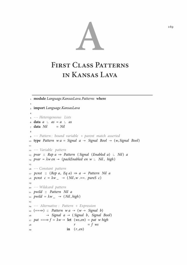
169

AFirst Class Patterns

in Kansas Lava

1 module Language.KansasLava.Patterns where2

3 import Language.KansasLava4

5 −− Heterogeneous Lists6 data a :. as = a :. as7 data Nil = Nil8

9 −− Pattern : bound variable + parent match asserted10 type Pattern w a = Signal a → Signal Bool → (w, Signal Bool)11

12 −− Variable pattern13 pvar :: Rep a ⇒ Pattern ( Signal (Enabled a) :. Nil ) a14 pvar = λw en → (packEnabled en w :. Nil , high )15

16 −− Constant pattern17 pcnst :: (Rep a , Eq a) ⇒ a → Pattern Nil a18 pcnst c = λw _ → (Nil ,w .==. pureS c)19

20 −−Wildcard pattern21 pwild :: Pattern Nil a22 pwild = λw _ → (Nil , high )23

24 −− Alternative : Pattern + Expression25 (==⇒) :: Pattern w a → (w → Signal b)26 → Signal a → ( Signal b , Signal Bool)27 pat ==⇒ f = λw→ let (ws,en) = pat w high28 r = f ws29 in (r ,en)

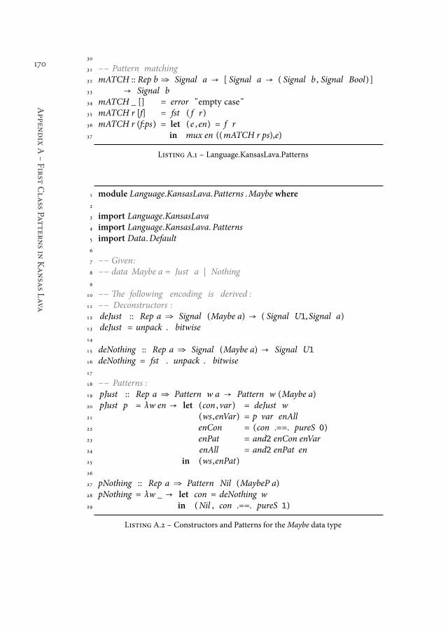
170

Appen

dix

AśFirst

Cla

ssPat

ternsin

KansasLava

30

31 −− Pattern matching32 mATCH :: Rep b ⇒ Signal a → [ Signal a → ( Signal b , Signal Bool) ]33 → Signal b34 mATCH _ [] = error "empty case "35 mATCH r [f] = fst ( f r)36 mATCH r (f:ps) = let (e ,en) = f r37 in mux en ((mATCH r ps),e)

Listing A.1 ś Language.KansasLava.Patterns

1 module Language.KansasLava.Patterns .Maybe where2

3 import Language.KansasLava4 import Language.KansasLava. Patterns5 import Data.Default6

7 −− Given:8 −− data Maybe a = Just a | Nothing9

10 −−he following encoding is derived :11 −− Deconstructors :12 deJust :: Rep a ⇒ Signal (Maybe a) → ( Signal U1,Signal a)13 deJust = unpack . bitwise14

15 deNothing :: Rep a ⇒ Signal (Maybe a) → Signal U116 deNothing = fst . unpack . bitwise17

18 −− Patterns :19 pJust :: Rep a ⇒ Pattern w a → Pattern w (Maybe a)20 pJust p = λw en → let (con , var) = deJust w21 (ws,enVar) = p var enAll22 enCon = (con .==. pureS 0)23 enPat = and2 enCon enVar24 enAll = and2 enPat en25 in (ws,enPat)26

27 pNothing :: Rep a ⇒ Pattern Nil (MaybeP a)28 pNothing = λw _ → let con = deNothing w29 in (Nil , con .==. pureS 1)

Listing A.2 ś Constructors and Patterns for theMaybe data type

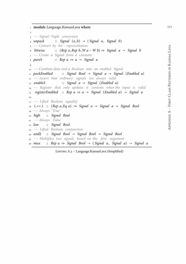
171

Appen

dix

AśFirst

Cla

ssPatternsin

KansasLava

1 module Language.KansasLava where2

3 −− Signal /Tuple conversion4 unpack :: Signal (a ,b) → ( Signal a , Signal b)5 −− Convert by bit− representation6 bitwise :: (Rep a ,Rep b ,W a ~W b)⇒ Signal a → Signal b7 −− Create a Signal from a constant8 pureS :: Rep a ⇒ a → Signal a9

10 −− Combine data and a Boolean into an enabled Signal11 packEnabled :: Signal Bool → Signal a → Signal (Enabled a)12 −− Assert that ordinary signals are always valid13 enableS :: Signal a → Signal (Enabled a)14 −− Register that only updates it contents when the input is valid15 registerEnabled :: Rep a ⇒ a → Signal (Enabled a) → Signal a16

17 −− Lited Boolean equality18 (.==.) :: (Rep a ,Eq a) ⇒ Signal a → Signal a → Signal Bool19 −− Always ’True ’20 high :: Signal Bool21 −− Always ’ False ’22 low :: Signal Bool23 −− Lited Boolean conjunction24 and2 :: Signal Bool → Signal Bool → Signal Bool25 −− Multiplex two signals based on the irst argument26 mux :: Rep a ⇒ Signal Bool → ( Signal a , Signal a) → Signal a

Listing A.3 ś Language.KansasLava (Simpliied)

172

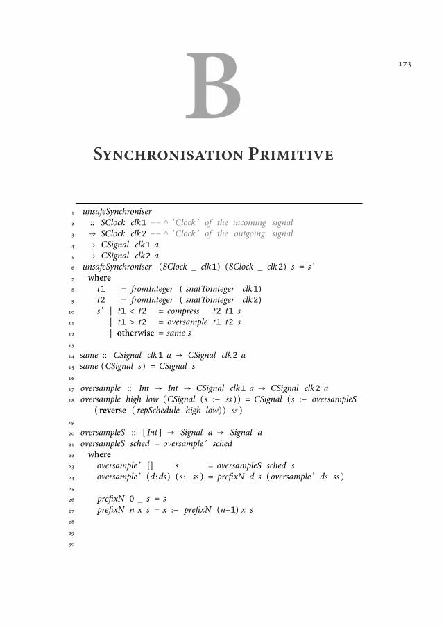
173

BSynchronisation Primitive

1 unsafeSynchroniser2 :: SClock clk1 −− ^ ’Clock ’ of the incoming signal3 → SClock clk2 −− ^ ’Clock ’ of the outgoing signal4 → CSignal clk1 a5 → CSignal clk2 a6 unsafeSynchroniser (SClock _ clk1) (SClock _ clk2) s = s ’7 where8 t1 = fromInteger ( snatToInteger clk1)9 t2 = fromInteger ( snatToInteger clk2)

10 s ’ | t1 < t2 = compress t2 t1 s11 | t1 > t2 = oversample t1 t2 s12 | otherwise = same s13

14 same :: CSignal clk1 a → CSignal clk2 a15 same (CSignal s ) = CSignal s16

17 oversample :: Int → Int → CSignal clk1 a → CSignal clk2 a18 oversample high low (CSignal ( s :− ss ) ) = CSignal ( s :− oversampleS

( reverse ( repSchedule high low)) ss )19

20 oversampleS :: [ Int ] → Signal a → Signal a21 oversampleS sched = oversample ’ sched22 where23 oversample ’ [] s = oversampleS sched s24 oversample ’ (d :ds) ( s :− ss ) = preixN d s (oversample ’ ds ss )25

26 preixN 0 _ s = s27 preixN n x s = x :− preixN (n−1) x s28

29

30

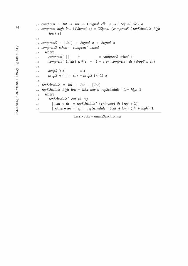
174

Appen

dix

BśSynchronisat

ionPrim

itive

31 compress :: Int → Int → CSignal clk1 a → CSignal clk2 a32 compress high low (CSignal s ) = CSignal (compressS ( repSchedule high

low) s )33

34 compressS :: [ Int ] → Signal a → Signal a35 compressS sched = compress ’ sched36 where37 compress ’ [] s = compressS sched s38 compress ’ (d :ds) ss@(s :− _) = s :− compress ’ ds (dropS d ss )39

40 dropS 0 s = s41 dropS n (_ :− ss ) = dropS (n−1) ss42

43 repSchedule :: Int → Int → [ Int ]44 repSchedule high low = take low $ repSchedule ’ low high 1

45 where46 repSchedule ’ cnt th rep47 | cnt < th = repSchedule ’ ( cnt+low) th ( rep + 1)48 | otherwise = rep : repSchedule ’ ( cnt + low) ( th + high ) 1

Listing B.1 ś unsafeSynchroniser

175

176

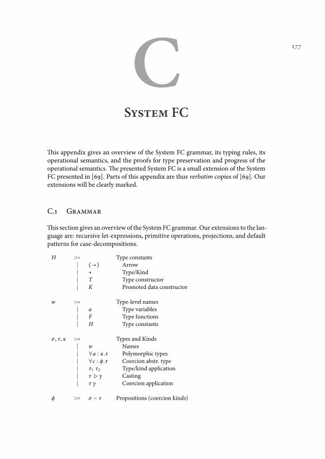
177

CSystem FC

his appendix gives an overview of the System FC grammar, its typing rules, itsoperational semantics, and the proofs for type preservation and progress of theoperational semantics. he presented System FC is a small extension of the SystemFC presented in [69]. Parts of this appendix are thus verbatim copies of [69]. Ourextensions will be clearly marked.

C.1 Grammar

his section gives an overview of the SystemFC grammar. Our extensions to the lan-guage are: recursive let-expressions, primitive operations, projections, and defaultpatterns for case-decompositions.

H ∶∶≙ Type constants∣ (→) Arrow∣ ⋆ Type/Kind∣ T Type constructor∣ K Promoted data constructor

w ∶∶≙ Type-level names∣ a Type variables∣ F Type functions∣ H Type constants

σ , τ, κ ∶∶≙ Types and Kinds∣ w Names∣ ∀a ∶ κ.τ Polymorphic types∣ ∀c ∶ ϕ.τ Coercion abstr. type∣ τ1 τ2 Type/kind application∣ τ▷ γ Casting∣ τ γ Coercion application

ϕ ∶∶≙ σ ∼ τ Propositions (coercion kinds)

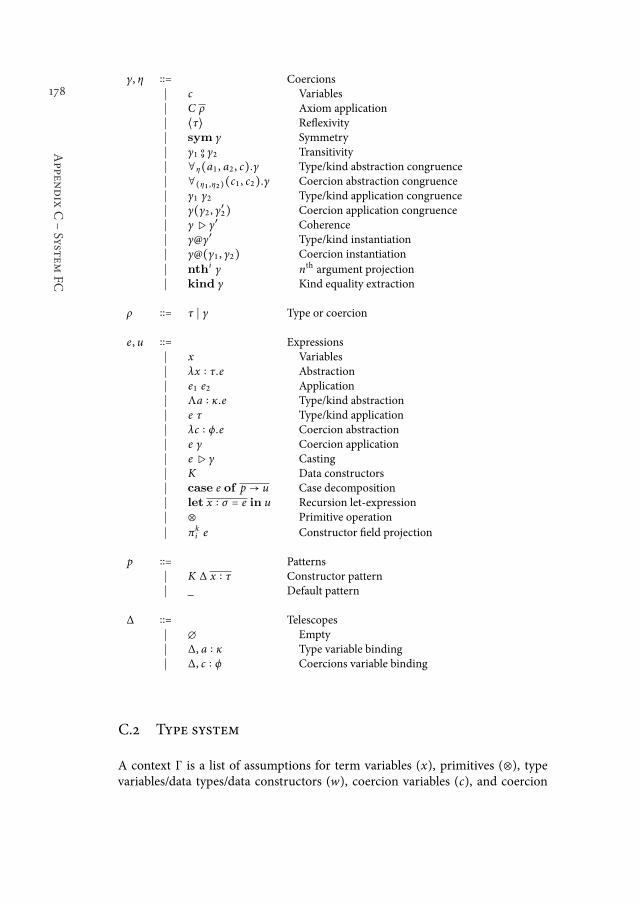
178

Appen

dix

CśSyst

emFC

γ, η ∶∶≙ Coercions∣ c Variables∣ C ρ Axiom application∣ ⟨τ⟩ Relexivity∣ sym γ Symmetry∣ γ1 o

9 γ2 Transitivity∣ ∀η(a1 , a2 , c).γ Type/kind abstraction congruence∣ ∀(η1 ,η2)(c1 , c2).γ Coercion abstraction congruence∣ γ1 γ2 Type/kind application congruence∣ γ(γ2 , γ

′2) Coercion application congruence

∣ γ▷ γ′ Coherence∣ γ@γ′ Type/kind instantiation∣ γ@(γ1 , γ2) Coercion instantiation

∣ nthi γ nth argument projection∣ kind γ Kind equality extraction

ρ ∶∶≙ τ ∣ γ Type or coercion

e , u ∶∶≙ Expressions∣ x Variables∣ λx ∶ τ.e Abstraction∣ e1 e2 Application∣ Λa ∶ κ.e Type/kind abstraction∣ e τ Type/kind application∣ λc ∶ ϕ.e Coercion abstraction∣ e γ Coercion application∣ e▷ γ Casting∣ K Data constructors∣ case e of p → u Case decomposition∣ let x ∶ σ ≙ e in u Recursion let-expression∣ ⊗ Primitive operation

∣ πki e Constructor ield projection

p ∶∶≙ Patterns∣ K ∆ x ∶ τ Constructor pattern∣ _ Default pattern

∆ ∶∶≙ Telescopes∣ ∅ Empty∣ ∆, a ∶ κ Type variable binding∣ ∆, c ∶ ϕ Coercions variable binding

C.2 Type system

A context Γ is a list of assumptions for term variables (x), primitives (⊗), typevariables/data types/data constructors (w), coercion variables (c), and coercion

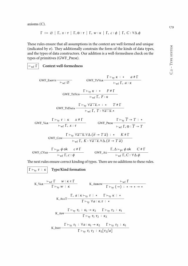
179

C.2śType

system

axioms (C).

Γ ∶∶≙ ∅ ∣ Γ, x ∶ τ ∣ Γ,⊗ ∶ τ ∣ Γ, w ∶ κ ∣ Γ, c ∶ ϕ ∣ Γ, C ∶ ∀∆.ϕ

hese rules ensure that all assumptions in the context are well formed and unique(indicated by #). hey additionally constrain the form of the kinds of data types,and the types of data constructors. Our addition is a well-formedness check on thetypes of primitives (GWF_Prim).

⊢wf Γ Context well-formedness

GWF_Empty⊢wf ∅

GWF_TyVarΓ ⊢ty κ ∶ ⋆ a # Γ

⊢wf Γ, a ∶ κ

GWF_TyFunΓ ⊢ty κ ∶ ⋆ F # Γ

⊢wf Γ, F ∶ κ

GWF_TyDataΓ ⊢ty ∀a ∶ κ.⋆ ∶ ⋆ T # Γ

⊢wf Γ, T ∶ ∀a ∶ κ.⋆

GWF_VarΓ ⊢ty τ ∶ κ x # Γ

⊢wf Γ, x ∶ τGWF_Prim

Γ ⊢ty T → T ∶ ⋆

⊢wf Γ,⊗ ∶ T → T

GWF_ConΓ ⊢ty ∀a ∶ κ.∀∆.(σ → T a) ∶ ⋆ K # Γ

⊢wf Γ, K ∶ ∀a ∶ κ.∀∆.(σ → T a)

GWF_CVarΓ ⊢pr ϕ ok c # Γ

⊢wf Γ, c ∶ ϕGWF_Ax

Γ, ∆ ⊢pr ϕ ok C # Γ

⊢wf Γ,C ∶ ∀∆.ϕ

henext rules ensure correct kinding of types. here are no additions to these rules.

Γ ⊢ty τ ∶ κ Type/Kind formation

K_Var⊢wf Γ w ∶ κ ∈ Γ

Γ ⊢ty w ∶ κK_Arrow

⊢wf Γ

Γ ⊢ty (→) ∶ ⋆→ ⋆→ ⋆

K_AllTΓ, a ∶ κ ⊢ty τ ∶ ⋆ Γ ⊢ty κ ∶ ⋆

Γ ⊢ty ∀a ∶ κ.τ ∶ ⋆

K_AppΓ ⊢ty τ1 ∶ κ1 → κ2 Γ ⊢ty τ2 ∶ κ1

Γ ⊢ty τ1 τ2 ∶ κ2

K_InstΓ ⊢ty τ1 ∶ ∀a ∶ κ1 → κ2 Γ ⊢ty τ2 ∶ κ1

Γ ⊢ty τ1 τ2 ∶ κ2∥τ2/a∥

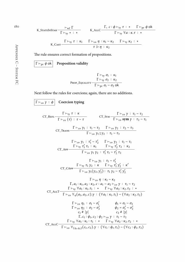
180

Appen

dix

CśSyst

emFC

K_StateInStar⊢wf Γ

Γ ⊢ty ⋆ ∶ ⋆K_AllC

Γ, c ∶ ϕ ⊢ty τ ∶ ⋆ Γ ⊢pr ϕ ok

Γ ⊢ty ∀a ∶ κ.τ ∶ ⋆

K_CastΓ ⊢ty τ ∶ κ1 Γ ⊢co η ∶ κ1 ∼ κ2 Γ ⊢ty κ2 ∶ ⋆

τ▷ η ∶ κ2

he rule ensures correct formation of propositions.

Γ ⊢pr ϕ ok Proposition validity

Prop_Equality

Γ ⊢ty σ1 ∶ κ1Γ ⊢ty σ2 ∶ κ2

Γ ⊢pr σ1 ∼ σ2 ok

Next follow the rules for coercions; again, there are no additions.

Γ ⊢co γ ∶ ϕ Coercion typing

CT_ReflΓ ⊢ty τ ∶ κ

Γ ⊢co ⟨τ⟩ ∶ τ ∼ τCT_Sym

Γ ⊢co γ ∶ τ1 ∼ τ2

Γ ⊢co sym γ ∶ τ2 ∼ τ1

CT_TransΓ ⊢co γ1 ∶ τ1 ∼ τ2 Γ ⊢co γ2 ∶ τ2 ∼ τ3

Γ ⊢co γ1 o9 γ2 ∶ τ1 ∼ τ3

CT_App

Γ ⊢co γ1 ∶ τ′1 ∼ τ

′2 Γ ⊢co γ2 ∶ τ1 ∼ τ1

Γ ⊢ty τ′1 τ1 ∶ κ1 Γ ⊢ty τ

′2 τ2 ∶ κ2

Γ ⊢co γ1 γ2 ∶ τ′1 τ1 ∼ τ

′2 τ2

CT_CApp

Γ ⊢co γ1 ∶ τ1 ∼ τ′1

Γ ⊢ty τ1 γ2 ∶ κ Γ ⊢ty τ′1 γ′2 ∶ κ

′

Γ ⊢co γ1(γ2 , γ′2) ∶ τ1 γ2 ∼ τ

′1 γ′2

CT_AllT

Γ ⊢co η ∶ κ1 ∼ κ2Γ, a1 ∶ κ1 , a2 ∶ κ2 , c ∶ a1 ∼ a2 ⊢co γ ∶ τ1 ∼ τ2

Γ ⊢ty ∀a1 ∶ κ1 .τ1 ∶ ⋆ Γ ⊢ty ∀a2 ∶ κ2 .τ2 ∶ ⋆

Γ ⊢co ∀η(a1 , a2 , c).γ ∶ (∀a1 ∶ κ1 .τ1) ∼ (∀a2 ∶ κ2 .τ2)

CT_AllC

Γ ⊢co η1 ∶ σ1 ∼ σ′1 ϕ1 ≙ σ1 ∼ σ2

Γ ⊢co η2 ∶ σ2 ∼ σ′2 ϕ2 ≙ σ ′1 ∼ σ

′2

c1 # ∣γ∣ c2 # ∣γ∣Γ, c1 ∶ ϕ1 , c2 ∶ ϕ2 ⊢co γ ∶ τ1 ∼ τ2

Γ ⊢ty ∀a1 ∶ κ1 ∶ τ1 ∶ ⋆ Γ ⊢ty ∀a2 ∶ κ2 .τ2 ∶ ⋆

Γ ⊢co ∀(η1 ,η2)(c1 , c2).γ ∶ (∀c1 ∶ ϕ1 .τ1) ∼ (∀c2 ∶ ϕ2 .τ2)

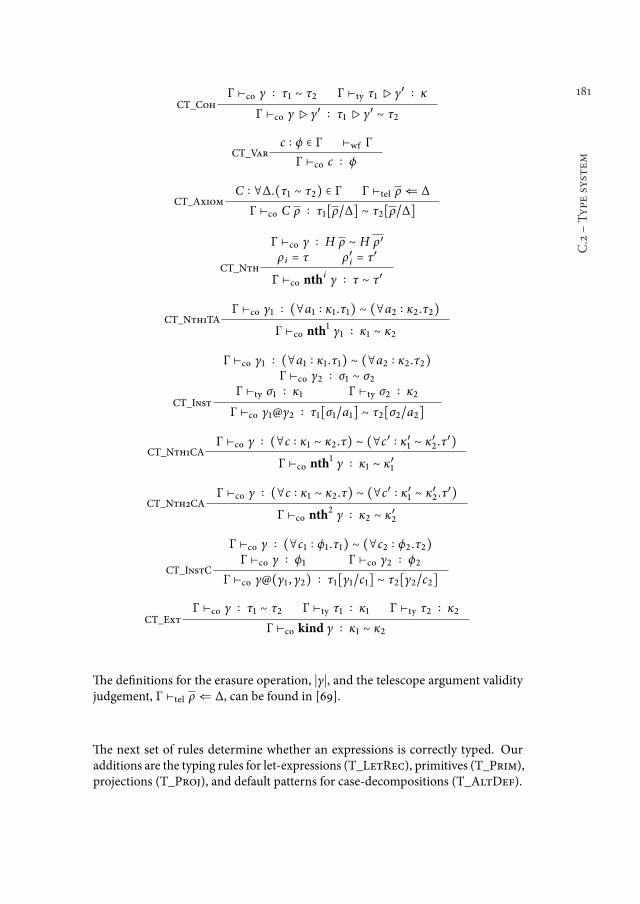
181

C.2śType

system

CT_CohΓ ⊢co γ ∶ τ1 ∼ τ2 Γ ⊢ty τ1 ▷ γ′ ∶ κ

Γ ⊢co γ▷ γ′ ∶ τ1 ▷ γ′ ∼ τ2

CT_Varc ∶ ϕ ∈ Γ ⊢wf Γ

Γ ⊢co c ∶ ϕ

CT_AxiomC ∶ ∀∆.(τ1 ∼ τ2) ∈ Γ Γ ⊢tel ρ ⇐ ∆

Γ ⊢co C ρ ∶ τ1∥ρ/∆∥ ∼ τ2∥ρ/∆∥

CT_Nth

Γ ⊢co γ ∶ H ρ ∼ H ρ′

ρ i ≙ τ ρ′i ≙ τ′

Γ ⊢co nthi γ ∶ τ ∼ τ′

CT_Nth1TAΓ ⊢co γ1 ∶ (∀a1 ∶ κ1 .τ1) ∼ (∀a2 ∶ κ2 .τ2)

Γ ⊢co nth1 γ1 ∶ κ1 ∼ κ2

CT_Inst

Γ ⊢co γ1 ∶ (∀a1 ∶ κ1 .τ1) ∼ (∀a2 ∶ κ2 .τ2)Γ ⊢co γ2 ∶ σ1 ∼ σ2

Γ ⊢ty σ1 ∶ κ1 Γ ⊢ty σ2 ∶ κ2

Γ ⊢co γ1@γ2 ∶ τ1∥σ1/a1∥ ∼ τ2∥σ2/a2∥

CT_Nth1CAΓ ⊢co γ ∶ (∀c ∶ κ1 ∼ κ2 .τ) ∼ (∀c

′ ∶ κ′1 ∼ κ′2 .τ′)

Γ ⊢co nth1 γ ∶ κ1 ∼ κ

′1

CT_Nth2CAΓ ⊢co γ ∶ (∀c ∶ κ1 ∼ κ2 .τ) ∼ (∀c

′ ∶ κ′1 ∼ κ′2 .τ′)

Γ ⊢co nth2 γ ∶ κ2 ∼ κ

′2

CT_InstC

Γ ⊢co γ ∶ (∀c1 ∶ ϕ1 .τ1) ∼ (∀c2 ∶ ϕ2 .τ2)Γ ⊢co γ ∶ ϕ1 Γ ⊢co γ2 ∶ ϕ2

Γ ⊢co γ@(γ1 , γ2) ∶ τ1∥γ1/c1∥ ∼ τ2∥γ2/c2∥

CT_Ext

Γ ⊢co γ ∶ τ1 ∼ τ2 Γ ⊢ty τ1 ∶ κ1 Γ ⊢ty τ2 ∶ κ2

Γ ⊢co kind γ ∶ κ1 ∼ κ2

he deinitions for the erasure operation, ∣γ∣, and the telescope argument validityjudgement, Γ ⊢tel ρ ⇐ ∆, can be found in [69].

he next set of rules determine whether an expressions is correctly typed. Ouradditions are the typing rules for let-expressions (T_LetRec), primitives (T_Prim),projections (T_Proj), and default patterns for case-decompositions (T_AltDef).

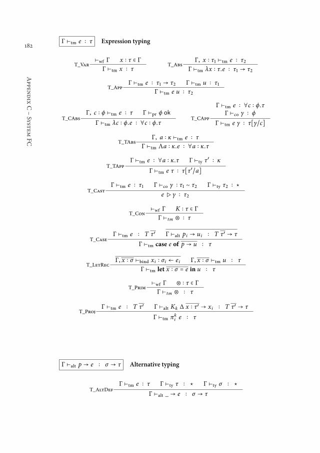
182

Appen

dix

CśSyst

emFC

Γ ⊢tm e ∶ τ Expression typing

T_Var⊢wf Γ x ∶ τ ∈ Γ

Γ ⊢tm x ∶ τT_Abs

Γ, x ∶ τ1 ⊢tm e ∶ τ2Γ ⊢tm λx ∶ τ.e ∶ τ1 → τ2

T_AppΓ ⊢tm e ∶ τ1 → τ2 Γ ⊢tm u ∶ τ1

Γ ⊢tm e u ∶ τ2

T_CAbsΓ, c ∶ ϕ ⊢tm e ∶ τ Γ ⊢pr ϕ ok

Γ ⊢tm λc ∶ ϕ.e ∶ ∀c ∶ ϕ.τT_CApp

Γ ⊢tm e ∶ ∀c ∶ ϕ.τΓ ⊢co γ ∶ ϕ

Γ ⊢tm e γ ∶ τ∥γ/c∥

T_TAbsΓ, a ∶ κ ⊢tm e ∶ τ

Γ ⊢tm Λa ∶ κ.e ∶ ∀a ∶ κ.τ

T_TAppΓ ⊢tm e ∶ ∀a ∶ κ.τ Γ ⊢ty τ

′ ∶ κ

Γ ⊢tm e τ ∶ τ∥τ′/a∥

T_CastΓ ⊢tm e ∶ τ1 Γ ⊢co γ ∶ τ1 ∼ τ2 Γ ⊢ty τ2 ∶ ⋆

e▷ γ ∶ τ2

T_Con⊢wf Γ K ∶ τ ∈ Γ

Γ ⊢tm ⊗ ∶ τ

T_CaseΓ ⊢tm e ∶ T τ′ Γ ⊢alt p i → u i ∶ T τ′ → τ

Γ ⊢tm case e of p → u ∶ τ

T_LetRecΓ, x ∶ σ ⊢bind x i ∶ σi ← e i Γ, x ∶ σ ⊢tm u ∶ τ

Γ ⊢tm let x ∶ σ ≙ e in u ∶ τ

T_Prim⊢wf Γ ⊗ ∶ τ ∈ Γ

Γ ⊢tm ⊗ ∶ τ

T_ProjΓ ⊢tm e ∶ T τ′ Γ ⊢alt Kk ∆ x ∶ τ′ → x i ∶ T τ′ → τ

Γ ⊢tm πki e ∶ τ

Γ ⊢alt p → e ∶ σ → τ Alternative typing

T_AltDefΓ ⊢tm e ∶ τ Γ ⊢ty τ ∶ ⋆ Γ ⊢ty σ ∶ ⋆

Γ ⊢alt _→ e ∶ σ → τ

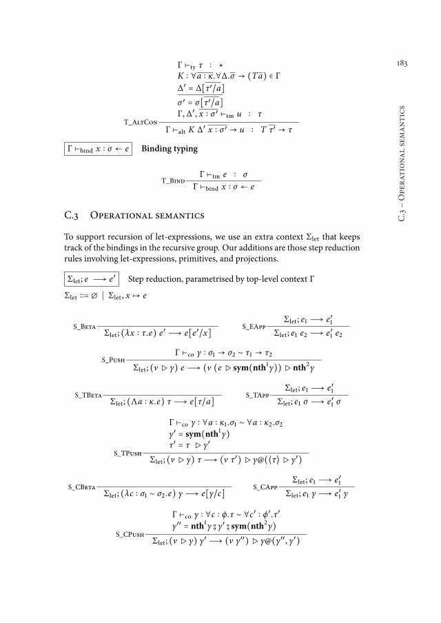
183

C.3śOperat

ionalsemantics

T_AltCon

Γ ⊢ty τ ∶ ⋆K ∶ ∀a ∶ κ.∀∆.σ → (Ta) ∈ Γ

∆′ ≙ ∆∥τ′/a∥

σ ′ ≙ σ∥τ′/a∥Γ, ∆′ , x ∶ σ ′ ⊢tm u ∶ τ

Γ ⊢alt K ∆′ x ∶ σ ′ → u ∶ T τ′ → τ

Γ ⊢bind x ∶ σ ← e Binding typing

T_BindΓ ⊢tm e ∶ σ

Γ ⊢bind x ∶ σ ← e

C.3 Operational semantics

To support recursion of let-expressions, we use an extra context Σlet that keepstrack of the bindings in the recursive group. Our additions are those step reductionrules involving let-expressions, primitives, and projections.

Σlet; e Ð→ e′ Step reduction, parametrised by top-level context Γ

Σlet ∶∶≙ ∅ ∣ Σlet , x ↦ e

S_BetaΣlet; (λx ∶ τ.e) e

′ Ð→ e∥e′/x∥S_EApp

Σlet; e1 Ð→ e′1Σlet; e1 e2 Ð→ e′1 e2

S_PushΓ ⊢co γ ∶ σ1 → σ2 ∼ τ1 → τ2

Σlet; (v▷ γ) e Ð→ (v (e▷ sym(nth1γ))▷ nth2γ

S_TBetaΣlet; (Λa ∶ κ.e) τ Ð→ e∥τ/a∥

S_TAppΣlet; e1 Ð→ e′1

Σlet; e1 σ Ð→ e′1 σ

S_TPush

Γ ⊢co γ ∶ ∀a ∶ κ1 .σ1 ∼ ∀a ∶ κ2 .σ2γ′ ≙ sym(nth1γ)τ′ ≙ τ ▷ γ′

Σlet; (v▷ γ) τ Ð→ (v τ′)▷ γ@(⟨τ⟩▷ γ′)

S_CBetaΣlet; (λc ∶ σ1 ∼ σ2 .e) γ Ð→ e∥γ/c∥

S_CAppΣlet; e1 Ð→ e′1

Σlet; e1 γ Ð→ e′1 γ

S_CPush

Γ ⊢co γ ∶ ∀c ∶ ϕ.τ ∼ ∀c′ ∶ ϕ′ .τ′

γ′′ ≙ nth1γ o9 γ′ o9 sym(nth

2γ)

Σlet; (v▷ γ) γ′ Ð→ (v γ′′)▷ γ@(γ′′ , γ′)

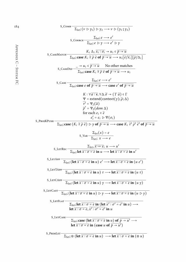
184

Appen

dix

CśSyst

emFC

S_CombΣlet; (v▷ γ1)▷ γ2 Ð→ v▷ (γ1 o

9 γ2)

S_CoerceΣlet; e Ð→ e′

Σlet; e▷ γ Ð→ e′▷ γ

S_CaseMatchK i ∆ i x i ∶ σi → u i ∈ p → u

Σlet; case K i τ ρ e of p → u Ð→ u i∥e/x i∥∥ρ/∆ i∥

S_CaseDef_→ u i ∈ p → u No other matches

Σlet; case K i τ ρ e of p → u Ð→ u i

S_CaseΣlet; e Ð→ e′

Σlet; case e of p → u Ð→ case e′ of p → u

S_ProjKPush

K ∶ ∀a ∶ κ.∀∆.σ → (T a) ∈ ΓΨ ≙ extend(context(γ); ρ;∆)τ′ ≙ Ψ2(a)ρ′ ≙ Ψ2(dom ∆)for each e i ∈ e

e′i ≙ e i ▷Ψ(σi)

Σlet; case (K i τ ρ e)▷ γ of p → u Ð→ case K i τ′ ρ′ e′ of p → u

S_VarΣlet(x) ≙ e

Σlet; x Ð→ e

S_LetRecΣlet , x ↦ e; u Ð→ u′

Σlet; let x ∶ σ ≙ e in u Ð→ let x ∶ σ ≙ e in u′

S_LetAppΣlet; (let x ∶ σ ≙ e in u) e′ Ð→ let x ∶ σ ≙ e in (u e′)

S_LetTAppΣlet; (let x ∶ σ ≙ e in u) τ Ð→ let x ∶ σ ≙ e in (u τ)

S_LetCAppΣlet; (let x ∶ σ ≙ e in u) γ Ð→ let x ∶ σ ≙ e in (u γ)

S_LetCastΣlet; (let x ∶ σ ≙ e in u)▷ γ Ð→ let x ∶ σ ≙ e in (u▷ γ)

S_LetFlat

Σlet; let x ∶ σ ≙ e in (let x′ ∶ σ ′ ≙ e′ in u)Ð→let x ∶ σ ≙ e , x′ ∶ σ ′ ≙ e′ in u

S_LetCase

Σlet; case (let x ∶ σ ≙ e in u) of p → u′ Ð→let x ∶ σ ≙ e in (case u of p → u′)

S_PrimLetΣlet;⊗ (let x ∶ σ ≙ e in u) Ð→ let x ∶ σ ≙ e in (⊗ u)

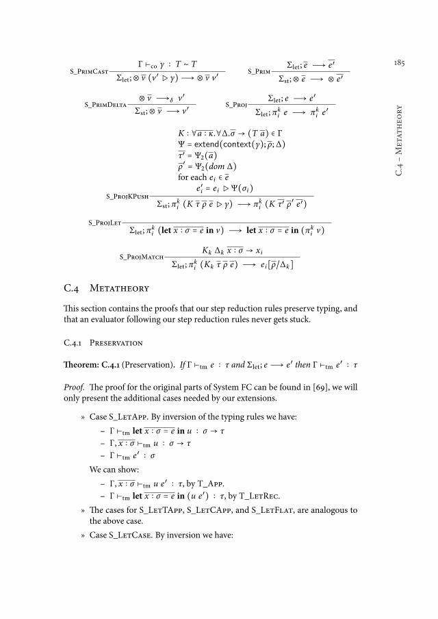
185

C.4śMetat

heo

ry

S_PrimCastΓ ⊢co γ ∶ T ∼ T

Σlet;⊗ v (v′▷ γ) Ð→ ⊗ v v′S_Prim

Σlet; e Ð→ e′

Σst;⊗ e Ð→ ⊗ e′

S_PrimDelta⊗ v Ð→δ v′

Σst;⊗ v Ð→ v′S_Proj

Σlet; e Ð→ e′

Σlet; πki e Ð→ πk

i e′

S_ProjKPush

K ∶ ∀a ∶ κ.∀∆.σ → (T a) ∈ ΓΨ ≙ extend(context(γ); ρ;∆)τ′ ≙ Ψ2(a)ρ′ ≙ Ψ2(dom ∆)for each e i ∈ e

e′i ≙ e i ▷Ψ(σi)

Σst; πki (K τ ρ e▷ γ) Ð→ πk

i (K τ′ ρ′ e′)

S_ProjLet

Σlet; πki (let x ∶ σ ≙ e in v) Ð→ let x ∶ σ ≙ e in (πk

i v)

S_ProjMatchKk ∆k x ∶ σ → x i

Σlet; πki (Kk τ ρ e) Ð→ e i∥ρ/∆k∥

C.4 Metatheory

his section contains the proofs that our step reduction rules preserve typing, andthat an evaluator following our step reduction rules never gets stuck.

C.4.1 Preservation

heorem: C.4.1 (Preservation). If Γ ⊢tm e ∶ τ and Σlet; e Ð→ e′ then Γ ⊢tm e′ ∶ τ

Proof. he proof for the original parts of System FC can be found in [69], we willonly present the additional cases needed by our extensions.

ż Case S_LetApp. By inversion of the typing rules we have:

ś Γ ⊢tm let x ∶ σ ≙ e in u ∶ σ → τ

ś Γ, x ∶ σ ⊢tm u ∶ σ → τ

ś Γ ⊢tm e′ ∶ σ

We can show:

ś Γ, x ∶ σ ⊢tm u e′ ∶ τ, by T_App.

ś Γ ⊢tm let x ∶ σ ≙ e in (u e′) ∶ τ, by T_LetRec.

ż he cases for S_LetTApp, S_LetCApp, and S_LetFlat, are analogous tothe above case.

ż Case S_LetCase. By inversion we have:

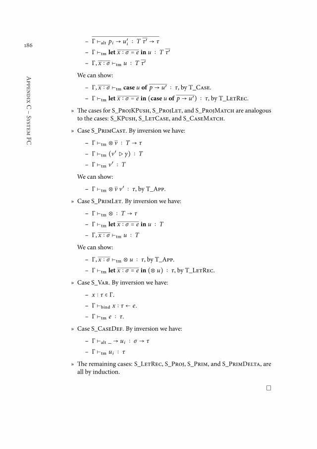
186

Appen

dix

CśSyst

emFC

ś Γ ⊢alt p i → u′i ∶ T τ′ → τ

ś Γ ⊢tm let x ∶ σ ≙ e in u ∶ T τ′

ś Γ, x ∶ σ ⊢tm u ∶ T τ′

We can show:

ś Γ, x ∶ σ ⊢tm case u of p → u′ ∶ τ, by T_Case.

ś Γ ⊢tm let x ∶ σ ≙ e in (case u of p → u′) ∶ τ, by T_LetRec.

ż he cases for S_ProjKPush, S_ProjLet, and S_ProjMatch are analogousto the cases: S_KPush, S_LetCase, and S_CaseMatch.

ż Case S_PrimCast. By inversion we have:

ś Γ ⊢tm ⊗ v ∶ T → τ

ś Γ ⊢tm (v′▷ γ) ∶ T

ś Γ ⊢tm v′ ∶ T

We can show:

ś Γ ⊢tm ⊗ v v′ ∶ τ, by T_App.

ż Case S_PrimLet. By inversion we have:

ś Γ ⊢tm ⊗ ∶ T → τ

ś Γ ⊢tm let x ∶ σ ≙ e in u ∶ T

ś Γ, x ∶ σ ⊢tm u ∶ T

We can show:

ś Γ, x ∶ σ ⊢tm ⊗ u ∶ τ, by T_App.

ś Γ ⊢tm let x ∶ σ ≙ e in (⊗ u) ∶ τ, by T_LetRec.

ż Case S_Var. By inversion we have:

ś x ∶ τ ∈ Γ.

ś Γ ⊢bind x ∶ τ ← e.

ś Γ ⊢tm e ∶ τ.

ż Case S_CaseDef. By inversion we have:

ś Γ ⊢alt _→ u i ∶ σ → τ

ś Γ ⊢tm u i ∶ τ

ż he remaining cases: S_LetRec, S_Proj, S_Prim, and S_PrimDelta, areall by induction.

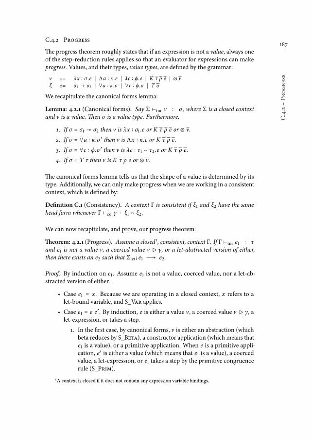
187

C.4.2śProgress

C.4.2 Progress

he progress theorem roughly states that if an expression is not a value, always oneof the step-reduction rules applies so that an evaluator for expressions can makeprogress. Values, and their types, value types, are deined by the grammar:

v ::= λx ∶ σ .e ∣ Λa ∶ κ.e ∣ λc ∶ ϕ.e ∣ K τ ρ e ∣ ⊗ vξ ::= σ1 → σ2 ∣ ∀a ∶ κ.σ ∣ ∀c ∶ ϕ.σ ∣ T σ

We recapitulate the canonical forms lemma:

Lemma: 4.2.1 (Canonical forms). Say Σ ⊢tm v ∶ σ , where Σ is a closed contextand v is a value. hen σ is a value type. Furthermore,

1. If σ ≙ σ1 → σ2 then v is λx ∶ σ1 .e or K τ ρ e or ⊗ v.

2. If σ ≙ ∀a ∶ κ.σ ′ then v is Λx ∶ κ.e or K τ ρ e.

3. If σ ≙ ∀c ∶ ϕ.σ ′ then v is λc ∶ τ1 ∼ τ2 .e or K τ ρ e.

4. If σ ≙ T τ then v is K τ ρ e or ⊗ v.

he canonical forms lemma tells us that the shape of a value is determined by itstype. Additionally, we can only make progress when we are working in a consistentcontext, which is deined by:

Deinition C.1 (Consistency). A context Γ is consistent if ξ1 and ξ2 have the samehead form whenever Γ ⊢co γ ∶ ξ1 ∼ ξ2.

We can now recapitulate, and prove, our progress theorem:

heorem: 4.2.1 (Progress). Assume a closed¹, consistent, context Γ. If Γ ⊢tm e1 ∶ τand e1 is not a value v, a coerced value v ▷ γ, or a let-abstracted version of either,then there exists an e2 such that Σlet; e1 Ð→ e2.

Proof. By induction on e1. Assume e1 is not a value, coerced value, nor a let-ab-stracted version of either.

ż Case e1 ≙ x. Because we are operating in a closed context, x refers to alet-bound variable, and S_Var applies.

ż Case e1 ≙ e e′. By induction, e is either a value v, a coerced value v ▷ γ, alet-expression, or takes a step.

1. In the irst case, by canonical forms, v is either an abstraction (whichbeta reduces by S_Beta), a constructor application (which means thate1 is a value), or a primitive application. When e is a primitive appli-cation, e′ is either a value (which means that e1 is a value), a coercedvalue, a let-expression, or e1 takes a step by the primitive congruencerule (S_Prim).

1A context is closed if it does not contain any expression variable bindings.

188

Appen

dix

CśSyst

emFC

ś When e′ is a coerced value (v▷γ), by the well-formedness check,primitives only operate on unparametrised data types and γ isa witness of the syntactical equality T ∼ T , and can be safelyremoved by (S_PrimCast).

ś When e′ is a let-expression, the let-binders are moved out of theapplication by PrimLet.

2. In the second case, we have a coercion between a value type τ, andτ1 → τ2. By consistency, then τ must be σ1 → σ2 and the S_Push ruleapplies.

3. In the third case, the let propagation rule for applications, S_LetApp,applies.

4. In the last case e1 takes a step by the application congruence rule S_-EApp.

ż Case e1 ≙ e τ and e1 ≙ e γ are analogous to the previous case moduloprimitives. By the well-formedness check, primitives are monomorphic.

ż Case e1 ≙ e▷ γ. By induction, either e is a value v, a coerced value v▷ γ, alet-expression, or takes a step.

1. In the irst case, then e1 is a coerced value.

2. In the second case, (v▷ γ′)▷ γ steps to v▷ (γ′ o9 γ) by S_Comb.

3. In the third case, the let propagation rule for casts, S_LetCast, applies.

4. In the last case, the congruence rule for casts, S_Coerce, applies.

ż Case e1 ≙ let x ∶ τ ≙ u in e. By induction, e is either a value v, a coercedvalue v▷ γ, a let-expression, or takes a step.

1. In the irst case, then e1 is a let-abstracted value.

2. In the second case, then e1 is a let-abstracted coerced value.

3. In the third case, the let-bindings are grouped into one let-expressionby S_LetFlat.

4. In the last case, the congruence rule for let expressions, S_LetRec,applies.

ż Case e1 ≙ case e of p → u. By induction, either e is a value v, a coercedvalue v▷ γ, a let-expression, or takes a step.

1. In the irst case, by canonical forms, v is either a constructor appli-cation and the case-decomposition reduces by S_CaseMatch or S_-CaseDef, or v is a primitive application, and e reduces by the ruleS_PrimDelta.

2. In the second case, we have a coercion γ between a value type τ, andT σ . By consistency, then τ must be T σ ′ and the KPush rule applies.

3. In the third case, the let-bindings are moved out of the case-decompo-sition by S_LetCase.

4. In the last case, the congruence rule for case-decompositions, S_Case,applies.

189

C.4.2śProgress

ż Case e1 ≙ πki e is analogous to the previous case.

190

191

DPreservation of

the rewrite rules

his appendix proves that the rewrite rules of chapter 4 are type and semanticspreserving.

D.1 Type preservation

For our proofs we will make use of the substitution lemma deined in [68]:

Lemma: D.1.1 (Term substitution). Say Γ1 ⊢tm e′ ∶ σ ′. If Γ1 , x ∶ σ′ , Γ2 ⊢tm e ∶ σ ,

then Γ1 , Γ2 ⊢tm e∥x ↦ e′∥ ∶ σ .

We need to show that the rewrite rules preserve the types of the expressions, andensure that binders added to the global environment Γ are correctly typed. We stateour type preservation theorem as follows:

heorem: D.1.1 (Type preservation). Given that for every expression binding in Γ,f i ∶ σi ≙ e i , Γ ⊢tm e i ∶ σi holds. If Γ ⊢tm e ∶ τ, and (Γ′ , e′) are the new environmentand the new expression ater applying a rewrite rule to e, then Γ′ ⊢tm e′ ∶ τ, and forevery f i ∶ σi ≙ e i in Γ′, Γ′ ⊢tm e i ∶ σi holds.

Proof. Many of the rewrite rules are a direct implementation of the operationalsemantics of System FC and are thus type preserving by theorem C.4.1, which isproven in the previous appendix.

We thus present the cases that are not a direct implementation of the operationalsemantics:

ż Case CaseTApp. By inversion of the typing rules we have:

ś Γ ⊢tm case e of p → u ∶ ∀a ∶ κ.τ

ś Γ ⊢alt p i → u i ∶ T τ′ → ∀a ∶ κ.τ

192

Appen

dix

DśPreservat

ionoftherew

riteru

les

ś Γ, ∆′ , x ∶ σ ′ ⊢tm u i ∶ ∀a ∶ κ.τ

ś Γ ⊢ty σ ∶ κ

We can show:

ś Γ, ∆′ , x ∶ σ ′ ⊢tm u i σ ∶ τ, by T_TApp.

ś Γ ⊢alt p i → (u i σ) ∶ T τ′ → τ, by T_AltCon.

ś Γ ⊢tm case e of p → (u σ) ∶ τ, by T_Case.

ż Cases CaseCApp and CaseCast are analogous to CaseTApp

ż Case LamApp. By inversion we have:

ś Γ ⊢tm λx ∶ σ .e ∶ σ → τ

ś Γ, x ∶ σ ⊢tm e ∶ τ

ś Γ ⊢tm u ∶ σ

We can show:

ś Γ ⊢bind x ∶ σ ← u, by T_Bind.

ś Γ ⊢tm let {x ∶ σ ≙ u} in e ∶ τ, by T_LetRec.

ż Case CaseApp. By inversion we have:

ś Γ ⊢tm case e of p → u ∶ σ → τ

ś Γ ⊢alt p i → u i ∶ T τ′ → (σ → τ)

ś Γ, ∆′ , x′ ∶ σ ′ ⊢tm u i ∶ σ → τ

ś Γ ⊢tm e′ ∶ σ

We can show:

ś Γ, , ∆′ , x′ ∶ σ ′ , x ∶ σ ⊢tm u i x ∶ τ, by T_App.

ś Γ, x ∶ σ ⊢alt p i → (u i x) ∶ T τ′ → τ, by T_AltCon.

ś Γ, x ∶ σ ⊢tm case e of p → (u x) ∶ τ, by T_Case.

ś Γ ⊢bind x ∶ σ ← e′, by T_Bind.

ś Γ ⊢tm let {x ∶ σ ≙ e′} in (case e of p → (u x)) ∶ τ, by T_LetRec.

ż Case BindNonRep. By inversion we have:

ś Γ, Γb, x i ∶ σi ⊢tm u ∶ τ, where Γ

brepresents all let-binders except

x i ∶ σi .

We can show:

ś Γ, x i ∶ σi ⊢tm let {b1; ...; b i−1; b i+1; ...; bn} in u ∶ τ, by T_LetRec.

ś Γ ⊢tm (let {b1; ...; b i−1; b i+1; ...; bn} in u)∥e i/x i∥ ∶ τ, by the substitu-tion lemma (lemma D.1.1).

ż Case LiftNonRep. By inversion we have:

ś Γ, Γb, x i ∶ σi ⊢tm u ∶ τ, where Γ

brepresents all let-binders except

x i ∶ σi .

We can show:

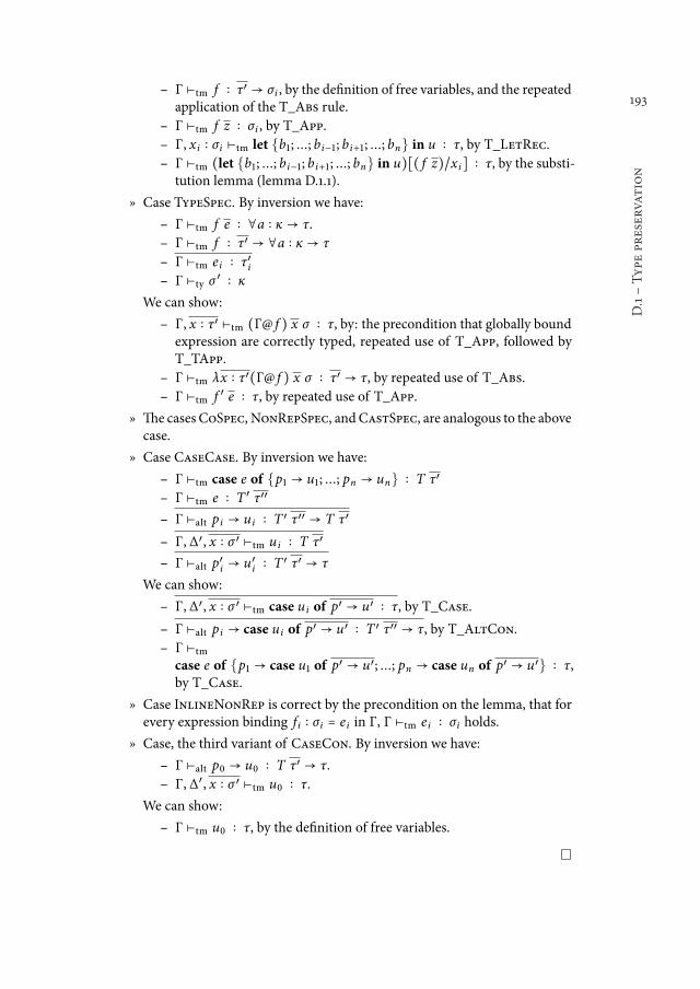
193

D.1śType

preservation

ś Γ ⊢tm f ∶ τ′ → σi , by the deinition of free variables, and the repeatedapplication of the T_Abs rule.

ś Γ ⊢tm f z ∶ σi , by T_App.ś Γ, x i ∶ σi ⊢tm let {b1; ...; b i−1; b i+1; ...; bn} in u ∶ τ, by T_LetRec.ś Γ ⊢tm (let {b1; ...; b i−1; b i+1; ...; bn} in u)∥( f z)/x i∥ ∶ τ, by the substi-tution lemma (lemma D.1.1).

ż Case TypeSpec. By inversion we have:

ś Γ ⊢tm f e ∶ ∀a ∶ κ → τ.ś Γ ⊢tm f ∶ τ′ → ∀a ∶ κ → τ

ś Γ ⊢tm e i ∶ τ′iś Γ ⊢ty σ

′ ∶ κ

We can show:

ś Γ, x ∶ τ′ ⊢tm (Γ@ f ) x σ ∶ τ, by: the precondition that globally boundexpression are correctly typed, repeated use of T_App, followed byT_TApp.

ś Γ ⊢tm λx ∶ τ′(Γ@ f ) x σ ∶ τ′ → τ, by repeated use of T_Abs.ś Γ ⊢tm f ′ e ∶ τ, by repeated use of T_App.

ż he casesCoSpec,NonRepSpec, andCastSpec, are analogous to the abovecase.

ż Case CaseCase. By inversion we have:

ś Γ ⊢tm case e of {p1 → u1; ...; pn → un} ∶ T τ′

ś Γ ⊢tm e ∶ T ′ τ′′

ś Γ ⊢alt p i → u i ∶ T ′ τ′′ → T τ′

ś Γ, ∆′ , x ∶ σ ′ ⊢tm u i ∶ T τ′

ś Γ ⊢alt p′i → u′i ∶ T′ τ′ → τ

We can show:

ś Γ, ∆′ , x ∶ σ ′ ⊢tm case u i of p′ → u′ ∶ τ, by T_Case.

ś Γ ⊢alt p i → case u i of p′ → u′ ∶ T ′ τ′′ → τ, by T_AltCon.ś Γ ⊢tm

case e of {p1 → case u1 of p′ → u′; ...; pn → case un of p′ → u′} ∶ τ,by T_Case.

ż Case InlineNonRep is correct by the precondition on the lemma, that forevery expression binding f i ∶ σi ≙ e i in Γ, Γ ⊢tm e i ∶ σi holds.

ż Case, the third variant of CaseCon. By inversion we have:

ś Γ ⊢alt p0 → u0 ∶ T τ′ → τ.ś Γ, ∆′ , x ∶ σ ′ ⊢tm u0 ∶ τ.

We can show:

ś Γ ⊢tm u0 ∶ τ, by the deinition of free variables.

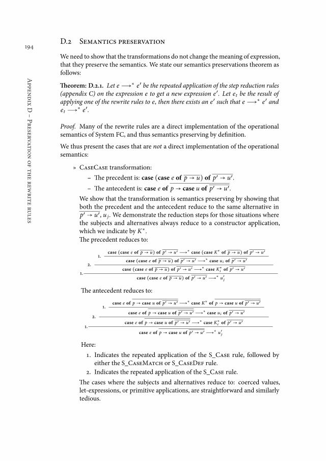
194

Appen

dix

DśPreservat

ionoftherew

riteru

les

D.2 Semantics preservation

We need to show that the transformations do not change themeaning of expression,that they preserve the semantics. We state our semantics preservations theorem asfollows:

heorem: D.2.1. Let e Ð→∗ e′ be the repeated application of the step reduction rules(appendix C) on the expression e to get a new expression e′. Let et be the result ofapplying one of the rewrite rules to e, then there exists an e′ such that e Ð→∗ e′ andet Ð→

∗ e′.

Proof. Many of the rewrite rules are a direct implementation of the operationalsemantics of System FC, and thus semantics preserving by deinition.

We thus present the cases that are not a direct implementation of the operationalsemantics:

ż CaseCase transformation:

ś he precedent is: case (case e of p → u) of p′ → u′.

ś he antecedent is: case e of p → case u of p′ → u′.

We show that the transformation is semantics preserving by showing thatboth the precedent and the antecedent reduce to the same alternative inp′ → u′, u j . We demonstrate the reduction steps for those situations wherethe subjects and alternatives always reduce to a constructor application,which we indicate by K∗.he precedent reduces to:

1.

2.

1.case (case e of p → u) of p′ → u′ Ð→∗ case (case K∗ of p → u) of p′ → u′

case (case e of p → u) of p′ → u′ Ð→∗ case u i of p′ → u′

case (case e of p → u) of p′ → u′ Ð→∗ case K∗i of p′ → u′

case (case e of p → u) of p′ → u′ Ð→∗ u′j

he antecedent reduces to:

1.

2.

1.case e of p → case u of p′ → u′ Ð→∗ case K∗ of p → case u of p′ → u′

case e of p → case u of p′ → u′ Ð→∗ case u i of p′ → u′

case e of p → case u of p′ → u′ Ð→∗ case K∗i of p′ → u′

case e of p → case u of p′ → u′ Ð→∗ u′j

Here:

1. Indicates the repeated application of the S_Case rule, followed byeither the S_CaseMatch or S_CaseDef rule.

2. Indicates the repeated application of the S_Case rule.

he cases where the subjects and alternatives reduce to: coerced values,let-expressions, or primitive applications, are straightforward and similarlytedious.

195

D.2śSemanticspreservation

ż he proofs for the other transformations are similarly straightforward andtedious.

196

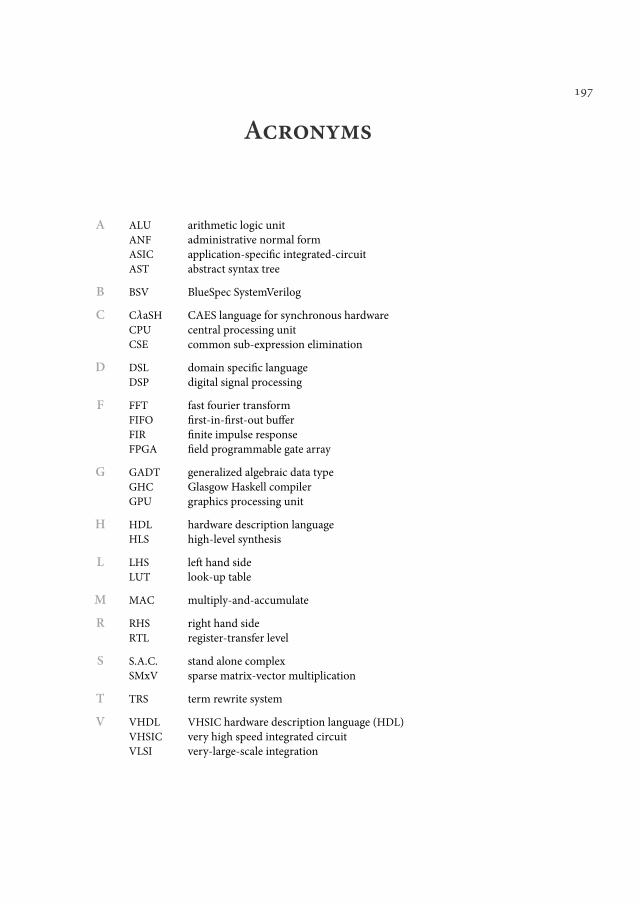
197

Acronyms

A ALU arithmetic logic unitANF administrative normal formASIC application-speciic integrated-circuitAST abstract syntax tree

B BSV BlueSpec SystemVerilog

C CλaSH CAES language for synchronous hardwareCPU central processing unitCSE common sub-expression elimination

D DSL domain speciic languageDSP digital signal processing

F FFT fast fourier transformFIFO irst-in-irst-out buferFIR inite impulse responseFPGA ield programmable gate array

G GADT generalized algebraic data typeGHC Glasgow Haskell compilerGPU graphics processing unit

H HDL hardware description languageHLS high-level synthesis

L LHS let hand sideLUT look-up table

M MAC multiply-and-accumulate

R RHS right hand sideRTL register-transfer level

S S.A.C. stand alone complexSMxV sparse matrix-vector multiplication

T TRS term rewrite system

V VHDL VHSIC hardware description language (HDL)VHSIC very high speed integrated circuitVLSI very-large-scale integration

198

199

Bibliography

[1] A. Acosta. ForSyDe tutorial. https://forsyde.ict.kth.se/trac/wiki/

ForSyDe/Haskell/ForSyDeTutorial, January 2011. (Cited on page 31).

[2] V. Akella and G. Gopalakrishnan. From Process-Oriented Functional Speciicationsto Eicient Asynchronous Circuits. In Proceedings of the 5th International Conferenceon VLSI Design, pages 324ś325. IEEE, January 1992. doi: 10.1109/ICVD.1992.658072.(Cited on page 7).

[3] P. J. Ashenden. he Designer’s Guide to VHDL. Morgan Kaufmann Publishers Inc.,San Francisco, CA, USA, 3rd edition, 2008. ISBN 978-0-12-088785-9. (Cited onpage 16).

[4] C. Baaij. CλasH: From Haskell To Hardware. Master’s thesis, University of Twente,December 2009. URL http://essay.utwente.nl/59482/. (Cited on page 13).

[5] H. Barendregt. he Lambda Calculus: Its Syntax and Semantics. Studies in Logic andthe Foundations of Mathematics. Elsevier Science, 1985. ISBN 978-0-08-093375-7.(Cited on page 25).

[6] J. M. Bell, F. Bellegarde, and J. Hook. Type-Driven Defunctionalization. In Proceed-ings of the 2nd International Conference on Functional Programming (ICFP), pages25ś37, 1997. doi: 10.1145/258948.258953. (Cited on page 98).

[7] P. Bjesse, K. Claessen, M. Sheeran, and S. Singh. Lava: Hardware Design in Haskell.In Proceedings of the 3rd International Conference on Functional Programming (ICFP),pages 174ś184. ACM, 1998. ISBN 1-58113-024-4. doi: 10.1145/289423.289440. (Citedon pages 10, 26, and 27).

[8] T. Bollaert. Catapult Synthesis: A Practical Introduction to Interactive C Synthesis.In P. Coussy and A. Morawiec, editors, High-Level Synthesis, pages 29ś52. SpringerNetherlands, 2008. ISBN 978-1-4020-8587-1. doi: 10.1007/978-1-4020-8588-8_3.(Cited on page 4).

[9] E. C. Brady. IDRIS Ð: Systems Programming Meets Full Dependent Types. In Pro-ceedings of the 5th Workshop on Programming Languages Meets Program Veriication(PLPV), PLPV ’11, pages 43ś54, New York, NY, USA, 2011. ACM. ISBN 978-1-4503-0487-0. doi: 10.1145/1929529.1929536. (Cited on page 62).

[10] R. K. Brayton, A. L. Sangiovanni-Vincentelli, C. T. McMullen, and G. D. Hachtel.Logic Minimization Algorithms for VLSI Synthesis. Kluwer Academic Publishers,Norwell, MA, USA, 1984. ISBN 0898381649. (Cited on page 91).

200

Biblio

graph

y

[11] M. M. T. Chakravarty, G. Keller, and S. P. Jones. Associated Type Synonyms. InProceedings of the 10th International Conference on Functional Programming (ICFP),ICFP ’05, pages 241ś253, New York, NY, USA, 2005. ACM. ISBN 1-59593-064-7. doi:10.1145/1086365.1086397. (Cited on pages 60 and 75).

[12] J. Cong, B. Liu, S. Neuendorfer, J. Noguera, K. Vissers, and Z. Zhang. High-LevelSynthesis for FPGAs: From Prototyping to Deployment. Computer-Aided Designof Integrated Circuits and Systems, IEEE Transactions on, 30(4):473ś491, April 2011.ISSN 0278-0070. doi: 10.1109/TCAD.2011.2110592. (Cited on page 6).

[13] P. Coussy, D. D. Gajski, M. Meredith, and A. Takach. An Introduction to High-LevelSynthesis. IEEE Design & Test of Computers, 26(4):8ś17, 2009. ISSN 0740-7475. doi:10.1109/MDT.2009.69. (Cited on page 3).

[14] Design, Automation&Test in Europe (DATE) conference. University Booth 2011 Pro-gramme. http://www.date­conference.com/date11/node/4165, March 2011.(Cited on page 141).

[15] R. A. Eisenberg and S. Weirich. Dependently Typed Programming with Singletons.In Proceedings of the 2012 Haskell Symposium, Haskell ’12, pages 117ś130, New York,NY, USA, 2012. ACM. ISBN 978-1-4503-1574-6. doi: 10.1145/2364506.2364522. (Citedon page 62).

[16] R. A. Eisenberg, D. Vytiniotis, S. Peyton Jones, and S. Weirich. Closed Type Familieswith Overlapping Equations. In Proceedings of the 41st Symposium on Principles ofProgramming Languages (POPL), pages 671ś683, New York, NY, USA, 2014. ACM.ISBN 978-1-4503-2544-8. doi: 10.1145/2535838.2535856. (Cited on page 75).

[17] S. Frankau. Hardware Synthesis from a Stream-Processing Functional Language. PhDthesis, University of Cambridge, July 2004. (Cited on page 72).

[18] M. Gerards, J. Kuper, A. Kokkeler, and B. Molenkamp. Streaming reduction circuit.In Proceedings of the 12th conference on Digital System Design (DSD), pages 287ś292,Los Alamitos, CA, USA, August 2009. IEEE Computer Society. ISBN 978-0-7695-3782-5. doi: 10.1109/DSD.2009.141. (Cited on pages 136 and 137).

[19] D. R. Ghica. Geometry of Synthesis: A structured approach to VLSI design. InProceedings of the 34th annual Symposium on Principles of Programming Languages(POPL), pages 363ś375. ACM, 2007. ISBN 1-59593-575-4. doi: 10.1145/1190216.1190269.(Cited on page 22).

[20] D. R. Ghica and A. Smith. Geometry of Synthesis II: From Games to Delay-Insensitive Circuits. In Proceedings of the 26th Conference on the Mathematical Foun-dations of Programming Semantics (MFPS), volume 265 of Electronic Notes in heo-retical Computer Science, pages 301ś324. 2010. doi: 10.1016/j.entcs.2010.08.018. (Notcited).

[21] D. R.Ghica andA. Smith. Geometry of Synthesis III: ResourceManagementhroughType Inference. In Proceedings of the 38th Symposium on Principles of Program-ming Languages (POPL), pages 345ś356. ACM, 2011. ISBN 978-1-4503-0490-0. doi:10.1145/1926385.1926425. (Cited on pages 22 and 24).

201

Bibliograph

y

[22] D. R. Ghica and A. Smith. Verity ś he Geometry of Synthesis. http://www.

veritygos.org, January 2013. (Cited on pages 22 and 67).

[23] D. R. Ghica, A. Smith, and S. Singh. Geometry of Synthesis IV: Compiling AineRecursion into Static Hardware. In Proceedings of the 16th International Conference onFunctional Programming (ICFP), pages 221ś233. ACM, 2011. ISBN 978-1-4503-0865-6.doi: 10.1145/2034773.2034805. (Cited on pages 22, 25, and 52).

[24] A. Gill. Type-Safe Observable Sharing in Haskell. In Proceedings of the 2nd HaskellSymposium, pages 117ś128. ACM, September 2009. ISBN 978-1-60558-508-6. doi:10.1145/1596638.1596653. (Cited on pages 10 and 27).

[25] A. Gill. kansas-lava: Kansas Lava is a hardware simulator and VHDL generator.http://hackage.haskell.org/package/kansas­lava, November 2011. (Citedon page 26).

[26] A. Gill, T. Bull, G. Kimmell, E. Perrins, E. Komp, and B. Werling. IntroducingKansas Lava. Submitted to he International Symposia on Implementation andApplication of Functional Languages (IFL), November 2009. URL http://ittc.

ku.edu/~andygill/papers/kansas­lava­ifl09.pdf. (Cited on pages 26, 27,136, and 159).

[27] A. Gill, T. Bull, A. Farmer, G. Kimmell, and E. Komp. Types and Type Families forHardware Simulation and Synthesis. In R. Page, Z. Horváth, and V. Zsók, editors,Trends in Functional Programming, volume 6546 of Lecture Notes in Computer Science(LNCS), pages 118ś133. Springer Berlin Heidelberg, 2011. ISBN 978-3-642-22940-4.doi: 10.1007/978-3-642-22941-1_8. (Cited on pages 26 and 27).

[28] Haskell.org. Template Haskell Wiki. http://www.haskell.org/haskellwiki/

Template_Haskell, October 2013. (Cited on pages 27, 31, 144, and 145).

[29] R. Herveille. CORDIC core. http://opencores.org/project,cordic, Septem-ber 2014. (Cited on page 147).

[30] R. Herveille. I2C controller core. http://opencores.org/project,i2c, Septem-ber 2014. (Cited on pages 142, 147, and 159).

[31] J. C. Hoe and Arvind. Hardware Synthesis from Term Rewriting Systems. In Pro-ceedings of the 10th International Conference on VLSI, pages 595ś619, 1999. (Cited onpage 21).

[32] J. Hughes. Generalising Monads to Arrows. Science of Computer Programming, 37(1-3):67ś111, May 2000. ISSN 0167-6423. doi: 10.1016/S0167-6423(99)00023-4. (Citedon page 159).

[33] IEEE Standard. Verilog Hardware Description Language, 2005. (Cited on page 18).

[34] IEEE Standard. VHDL Language Reference Manual, 2008. (Cited on page 16).

[35] IEEE Standard. SystemVerilog ś Uniied Hardware Design, Speciication, and Verii-cation Language, 2012. (Cited on page 20).

202

Biblio

graph

y

[36] X. Jin. Implementation of the MUSIC Algorithm in CλaSH. Master’s thesis, June2014. URL http://essay.utwente.nl/65225/. (Cited on page 135).

[37] E. Kmett. Lenses, Folds and Traversals. http://lens.github.io, September 2014.(Cited on pages 144 and 165).

[38] M. Kooijman. Haskell as a higher order structural hardware description lan-guage. Master’s thesis, University of Twente, December 2009. URL http://essay.utwente.nl/59381/. (Cited on pages 13 and 59).

[39] J. Kuper and R. Wester. N Queens on an FPGA: Mathematics, Programming, orBoth? In Communicating Process Architectures (CPA), United Kingdom, August2014 (to appear). Open Channel Publishing. (Cited on page 136).

[40] S. Mac Lane. Categories for theWorkingMathematician. Number 5 in Graduate Textsin Mathematics. New York, 1971. ISBN 0387900357. (Cited on page 143).

[41] G. Martin and G. Smith. High-Level Synthesis: Past, Present, and Future.IEEE Design & Test of Computers, 26(4):18ś25, 2009. ISSN 0740-7475. doi:10.1109/MDT.2009.83. (Cited on pages 4 and 6).

[42] C. Mcbride and R. Paterson. Applicative Programming with Efects. Journalof Functional Programming, 18(1):1ś13, January 2008. ISSN 0956-7968. doi:10.1017/S0956796807006326. (Cited on pages 57 and 165).

[43] M. C. McFarland, A. C. Parker, and R. Camposano. he high-level synthesis ofdigital systems. Proceedings of the IEEE, 78(2):301ś318, 1990. ISSN 0018-9219. doi:10.1109/5.52214. (Cited on page 3).

[44] G. H. Mealy. A Method for Synthesizing Sequential Circuits. Bell SystemTechnical Journal, 34(5):1045ś1079, 1955. ISSN 1538-7305. doi: 10.1002/j.1538-7305.1955.tb03788.x. (Cited on pages 30 and 59).

[45] A. Megacz. Hardware Design with Generalized Arrows. In A. Gill and J. Hage,editors, Implementation and Application of Functional Languages, volume 7257 ofLecture Notes in Computer Science, pages 164ś180. Springer Berlin Heidelberg, 2012.ISBN 978-3-642-34406-0. doi: 10.1007/978-3-642-34407-7_11. (Cited on page 160).

[46] N. Mitchell and C. Runciman. Losing Functions without Gaining Data. In Proceed-ings of the 2nd Symposium on Haskell, pages 13ś24. ACM, September 2009. ISBN978-1-60558-508-6. (Cited on page 99).

[47] A. Mycrot and R. Sharp. A Statically Allocated Parallel Functional Language. InProceedings of the 27th International Colloquium on Automata, Languages and Pro-gramming (ICALP), volume 1853 of Lecture Notes in Computer Science (LNCS), pages37ś48. Springer-Verlag, 2000. ISBN 978-3-540-67715-4. doi: 10.1007/3-540-45022-X_5. (Cited on pages 21, 22, and 66).

[48] A. Niedermeier. A Fine-Grained Parallel Datalow-Inspired Architecture for Stream-ing Applications. PhD thesis, Univ. of Twente, Enschede, August 2014. (Cited onpage 136).

203

Bibliograph

y

[49] R. S. Nikhil. Bluespec: A General-Purpose Approach to High-Level Synthesis Basedon Parallel Atomic Transactions. In Philippe Coussy and Adam Morawiec, editor,High-Level Synthesis - From Algorithm to Digital Circuit, pages 129ś146. SpringerNetherlands, 2008. (Cited on page 20).

[50] OpenCores. WISHBONE System-on-Chip Interconnect. http://opencores.org/opencores,wishbone, June 2010. (Cited on page 142).

[51] B. O’Sullivan, J. Goerzen, and D. Stewart. Real World Haskell, chapter Mon-ads. O’Reilly Media, Inc., 2008. ISBN 978-0-596-51498-3. URL http://book.

realworldhaskell.org/read/monads.html. (Cited on pages 144 and 165).

[52] R. Paterson. A New Notation for Arrows. In Proceedings of the 6th InternationalConference on Functional Programming (ICFP), ICFP ’01, pages 229ś240, New York,NY, USA, 2001. ACM. ISBN 1-58113-415-0. doi: 10.1145/507635.507664. (Cited onpages 68 and 159).

[53] R. Paterson. Arrows and Computation. In JeremyGibbons andOege deMoor, editor,he Fun of Programming, pages 201ś222. Palgrave, 2003. (Cited on page 68).

[54] S. Peyton Jones and A. Santos. Compilation by Transformation in the GlasgowHaskell Compiler. In Functional Programming, Glasgow 1994, Workshops in Com-puting, pages 184ś204. Springer London, 1995. ISBN 978-3-540-19914-4. doi:10.1007/978-1-4471-3573-9_13. (Cited on page 99).

[55] R. Pope and B. Yorgey. irst-class-patterns: First class patterns and pat-tern matching, using type families. http://hackage.haskell.org/package/

first­class­patterns, July 2013. (Cited on pages 28 and 29).

[56] F. Pottier and N. Gauthier. Polymorphic Typed Defunctionalization. In Proceedingsof the 31st Symposium on Principles of Programming Languages (POPL), pages 89ś98.ACM, 2004. ISBN 1-58113-729-X. doi: 10.1145/964001.964009. (Cited on page 98).

[57] J. C. Reynolds. Deinitional Interpreters for Higher-Order Programming Languages.In Proceedings of the 25th ACM National Conference, pages 717 ś 740. ACM Press,1972. (Cited on page 98).

[58] I. Sander and A. Jantsch. SystemModeling and Transformational Design Reinementin ForSyDe. IEEE Transactions on Computer-Aided Design of Integrated Circuits andSystems, 23(1):17ś32, January 2004. (Cited on pages 30 and 159).

[59] R. Sharp and A. Mycrot. he FLaSH Compiler: Eicient Circuits from FunctionalSpeciications. Technical report, AT&T Research Laboratories Cambridge, 2000.(Cited on page 21).

[60] T. Sheard and S. Peyton Jones. Template meta-programming for Haskell. In Proceed-ings of the 2002 Workshop on Haskell, pages 1ś16. ACM, 2002. ISBN 1-58113-605-6.doi: 10.1145/581690.581691. (Cited on pages 27 and 31).

[61] J. R. Shewchuk. An introduction to the conjugate gradient method without theagonizing pain. Technical report, Pittsburgh, PA, USA, 1994. URL http://www.

cs.cmu.edu/~quake­papers/painless­conjugate­gradient.pdf. (Cited onpage 136).

204

Biblio

graph

y

[62] M. Sulzmann, M. M. T. Chakravarty, S. Peyton Jones, and K. Donnelly. System Fwith Type Equality Coercions. In Proceedings of the 2007 International Workshopon Types in Languages Design and Implementation (TLDI), pages 53ś66, New York,NY, USA, 2007. ACM. ISBN 1-59593-393-X. doi: 10.1145/1190315.1190324. (Cited onpages 74, 75, and 79).

[63] S. Sutheland, S. Davidmann, and P. Flacke. SystemVerilog for Design. Springer US,2nd edition, 2006. ISBN 978-0-387-36495-7. doi: 10.1007/0-387-36495-1. (Cited onpage 18).

[64] he GHC Team. he GHC Compiler, version 7.6.3. http://haskell.org/ghc,April 2013. (Cited on page 12).

[65] heGHCTeam. GHCAPI. http://www.haskell.org/ghc/docs/latest/html/libraries/ghc/index.html, September 2014. (Cited on pages 74 and 75).

[66] F. Van Nee. To a new hardware design methodology: A case study of the cochleamodel. Master’s thesis, March 2014. URL http://essay.utwente.nl/64835/.(Cited on page 135).

[67] J. E. Volder. he CORDIC Trigonometric Computing Technique. IRE Transactionson Electronic Computers, EC-8(3):330ś334, September 1959. ISSN 0367-9950. doi:10.1109/TEC.1959.5222693. (Cited on page 147).

[68] S. Weirich, D. Vytiniotis, S. Peyton Jones, and S. Zdancewic. Generative Type Ab-straction and Type-level Computation. In Proceedings of the 38th Annual Symposiumon Principles of Programming Languages (POPL), pages 227ś240, New York, NY,USA, 2011. ACM. ISBN 978-1-4503-0490-0. doi: 10.1145/1926385.1926411. (Cited onpages 74, 75, and 191).

[69] S. Weirich, J. Hsu, and R. A. Eisenberg. System FC with Explicit Kind Equality. InProceedings of the 18th International Conference on Functional Programming (ICFP),pages 275ś286, New York, NY, USA, 2013. ACM. ISBN 978-1-4503-2326-0. doi:10.1145/2500365.2500599. (Cited on pages 74, 75, 78, 80, 82, 86, 177, 181, and 185).

[70] R. Wester and J. Kuper. A space/time tradeof methodology using higher-order func-tions. In 22nd International Conference on Field Programmable Logic and Applications(FPL), pages 1ś2, USA, 2013. IEEE Computer Society. (Cited on page 136).

[71] R. Wester and J. Kuper. Design space exploration of a particle ilter using higher-order functions. In Reconigurable Computing: Architectures, Tools, and Applications,volume 8405 of Lecture Notes in Computer Science, pages 219ś226. Springer Verlag,London, United Kingdom, 2014. (Cited on page 135).

[72] R. Wester and J. Kuper. Deriving stencil hardware accelerators from a single higher-order function. In Communicating Process Architectures (CPA), United Kingdom,August 2014 (to appear). Open Channel Publishing. (Cited on page 135).

[73] R. Wester, D. Sarakiotis, E. Kooistra, and J. Kuper. Speciication of APERTIFPolyphase Filter Bank in CλaSH. In Communicating Process Architectures (CPA),pages 53ś64, United Kingdom, August 2012. Open Channel Publishing. (Cited onpage 135).

205

Bibliograph

y

[74] H. Xi, C. Chen, and G. Chen. Guarded Recursive Datatype Constructors. In Proceed-ings of the 30th Symposium on Principles of Programming Languages, pages 224ś235,New York, NY, USA, 2003. ACM. ISBN 1-58113-628-5. doi: 10.1145/604131.604150.(Cited on page 75).

[75] B. A. Yorgey, S. Weirich, J. Cretin, S. Peyton Jones, D. Vytiniotis, and J. P. Magalhães.Giving Haskell a Promotion. In Proceedings of the 8th Workshop on Types in LanguageDesign and Implementation (TLDI), TLDI ’12, pages 53ś66, New York, NY, USA, 2012.ACM. ISBN 978-1-4503-1120-5. doi: 10.1145/2103786.2103795. (Cited on pages 61, 74,and 75).

[76] S. Zeirov. HHDL: Hardware Description Language embedded in Haskell. http://hackage.haskell.org/package/HHDL, December 2011. (Cited on pages 28and 29).

[77] Z. Zhang, Y. Fan, W. Jiang, G. Han, C. Yang, and J. Cong. AutoPilot: A Platform-Based ESL Synthesis System. In P. Coussy and A. Morawiec, editors, High-LevelSynthesis, pages 99ś112. Springer Netherlands, 2008. ISBN 978-1-4020-8587-1. doi:10.1007/978-1-4020-8588-8_6. (Cited on page 4).

[78] G. Érdi. A Brainfuck CPU in FPGA. https://github.com/gergoerdi/

brainfuck­cpu­fpga, January 2013. (Cited on page 28).

206

207

List of Publications

[CB:1] C. P. R. Baaij, M. Kooijman, J. Kuper, M. E. T. Gerards, and E. Molenkamp. ToolDemonstration: CLasH - From Haskell to Hardware. In Proceedings of the 2nd

Symposium on Haskell, page 3. ACM, 2009. doi: 10.1145/1596638.1667736.

[CB:2] G. J. M. Smit, J. Kuper, and C. P. R. Baaij. A mathematical approach towards hard-ware design. In P. M. Athanas, J. Becker, J. Teich, and I. Verbauwhede, editors,Dagstuhl Seminar on Dynamically Reconigurable Architectures, number 10281 inDagstuhl Seminar Proceedings. Schloss Dagstuhl - Leibniz-Zentrum fuer Infor-matik, Germany, December 2010.

[CB:3] A. Niedermeier, R. Wester, K. C. Rovers, C. P. R. Baaij, J. Kuper, and G. J. M.Smit. Designing a datalow processor using CλaSH. In 28th Norchip Con-ference, page 69. IEEE Circuits and Systems Society, November 2010. doi:10.1109/NORCHIP.2010.5669445.

[CB:4] A. Niedermeier, R. Wester, C. P. R. Baaij, J. Kuper, and G. J. M. Smit. Compar-ing CλaSH and VHDL by implementing a datalow processor. In Proceedingsof the Workshop on PROGram for Research on Embedded Systems and Sotware(PROGRESS), pages 216ś221. Technology Foundation STW, November 2010.

[CB:5] J. Kuper,C.P.R. Baaij, M.Kooijman, andM. E. T.Gerards. Exercises in architecturespeciication using CλaSH. In Proceedings of Forum on Speciication and DesignLanguages (FDL), pages 178ś183. ECSI Electronic Chips & Systems design Initiative,September 2010. doi: 10.1049/ic.2010.0149.

[CB:6] M. E. T. Gerards, C. P. R. Baaij, J. Kuper, andM. Kooijman. Hiding State in CλaSHHardware Descriptions. In Preproceedings of the 22nd Symposium on Implementa-tion and Application of Functional Languages (IFL), pages 107ś119. Utrecht Univer-sity, August 2010.

[CB:7] C. P. R. Baaij, M. Kooijman, J. Kuper, W. A. Boeijink, andM. E. T. Gerards. CλaSH:Structural Descriptions of Synchronous Hardware using Haskell. In Proceedings ofthe 13th Conference on Digital System Design (DSD), pages 714ś721. IEEE ComputerSociety, September 2010. doi: 10.1109/DSD.2010.21.

[CB:8] J. Kuper, C. P. R. Baaij, M. Kooijman, and M. E. T. Gerards. Architecture Speciica-tions in CλaSH. In T. J. Kaźmierski and A. Morawiec, editors, System SpeciicationandDesign Languages, volume 106 of LectureNotes in Electrical Engineering (LNEE),pages 191ś206. Springer New York, December 2011. doi: 10.1007/978-1-4614-1427-8_12.

208

List

ofPublic

ations

[CB:9] M. E. T. Gerards, C. P. R. Baaij, J. Kuper, andM. Kooijman. Higher-Order Abstrac-tion in Hardware Descriptions with CλaSH. In P. Kitsos, editor, Proceedings of the14th Conference on Digital System Design (DSD), pages 495ś502. IEEE ComputerSociety, August 2011. doi: 10.1109/DSD.2011.69.

[CB:10] C. P. R. Baaij, J. Kuper, and L. Schubert. SoOSiM: Operating System and Program-ming Language Exploration. In G. Lipari and T. Cucinotta, editors, Proceedings ofthe 3rd International Workshop on Analysis Tools and Methodologies for Embeddedand Real-time System (WATERS), pages 63ś68, 2012.

[CB:11] R. Wester, C. P. R. Baaij, and J. Kuper. A two step hardware design method us-ing CλaSH. In 22nd International Conference on Field Programmable Logic andApplications (FPL), pages 181ś188. IEEE Computer Society, August 2012. doi:10.1109/FPL.2012.6339258.

[CB:12] B. N. Uchevler, K. Svarstad, J. Kuper, andC. P. R. Baaij. System-Level Modelling ofDynamic Reconigurable Designs using Functional Programming Abstractions. In14th International Symposium on Quality Electronic Design (ISQED), pages 379ś385.IEEE, March 2013. doi: 10.1109/ISQED.2013.6523639.

[CB:13] C.P.R. Baaij and J. Kuper. Using Rewriting to Synthesize Functional Languagesto Digital Circuits. In Jay McCarthy, editor, Trends in Functional Programming(TFP), Provo, UT, USA, May 14-16, 2013, Revised Selected Papers, volume 8322 ofLectureNotes in Computer Science (LNCS), pages 17ś33. Springer-Verlag, 2014. ISBN978-3-642-45339-7. doi: 10.1007/978-3-642-45340-3_2.

This thesis

@phdthesis{baaij2015:thesis,

author={Baaij, Christiaan P.R.},

title={Digital Circuits in CλaSH ­­ FunctionalSpecifications and Type­Directed Synthesis},

school={Universiteit Twente},

address={PO Box 217, 7500AE Enschede, The Netherlands},

year={2015},

month={jan},

day={23},

number={CTIT Ph.D.­thesis series No. 14­335},

issn={1381­3617},

isbn={978­90­365­3803­9},

doi={10.3990/1.9789036538039}

}

209

CASHלועה םע םג הז לכ ,ןדעה ןגב ולש םיהולא

ם

λλ λ

λ

λλ

ISBN 978-90-365-3803-9

9 789036 538039