EC3062 ECONOMETRICS

HYPOTHESIS TESTS FOR THE CLASSICAL LINEAR MODEL

The Normal Distribution and the Sampling Distributions

To denote that x is a normally distributed random variable with a meanof E(x) = µ and a dispersion matrix of D(x) = Σ, we shall write x ∼N(µ,Σ).

A standard normal vector z ∼ N(0, I) has E(x) = 0 and D(x) = I.Any normal vector x ∼ N(µ,Σ) can be standardised:

(1) If T is a transformation such that TΣT ′ = I and T ′T = Σ−1,then T (x − µ) ∼ N(0, I).

If z ∼ N(0, I) is a standard normal vector of n elements, then the sum ofsquares of its elements has a chi-square distribution of n degrees of freedom;and this is denoted by z′z ∼ χ2(n). With the help of the standardisingtransformation, it can be shown that,

(2) If x ∼ N(µ,Σ) is a vector of order n, then

(x − µ)′Σ−1(x − µ) ∼ χ2(n).

1

EC3062 ECONOMETRICS

(3) If u ∼ χ2(m) and v ∼ χ2(n) are independent chi-square variatesof m and n degrees of freedom respectively, then (u + v) ∼χ2(m + n) is a chi-square variate of m + n degrees of freedom.

The ratio of two independent chi-square variates divided by their respectivedegrees of freedom has a F distribution. Thus,

(4) If u ∼ χ2(m) and v ∼ χ2(n) are independent chi-square vari-ates, then F = (u/m)/(v/n) has an F distribution of m and ndegrees of freedom; and this is denoted by writing F ∼ F (m, n).

A t variate is a ratio of a standard normal variate and the root of an inde-pendent chi-square variate divided by its degrees of freedom. Thus,

(5) If z ∼ N(0, 1) and v ∼ χ2(n) are independent variates, thent = z/

√(v/n) has a t distribution of n degrees of freedom; and

this is denoted by writing t ∼ t(n).

It is clear that t2 ∼ F (1, n).

2

EC3062 ECONOMETRICS

Hypothesis Concerning the Coefficients

The OLS estimate β = (X ′X)−1X ′y of β in the model (y;Xβ, σ2I) hasE(β̂) = β and D(β̂) = σ2(X ′X)−1, Thus, if y ∼ N(Xβ, σ2I), then

(6) β̂ ∼ Nk{β, σ2(X ′X)−1}.

Likewise, the marginal distributions of β̂1, β̂2 within β̂′ = [β̂1, β̂2] are givenby

β̂1 ∼ Nk1

(β1, σ

2{X ′1(I − P2)X1}−1

), P2 = X2(X ′

2X2)−1X2,(7)

β̂2 ∼ Nk2

(β2, σ

2{X ′2(I − P1)X2}−1

), P1 = X1(X ′

1X1)−1X1.(8)

From the results under (2) to (6), it follows that

(9) σ−2(β̂ − β)′X ′X(β̂ − β) ∼ χ2(k).

Similarly, it follows from (7) and (8) that

σ−2(β̂1 − β1)′X ′1(I − P2)X1(β̂1 − β1) ∼ χ2(k1),(10)

σ−2(β̂2 − β2)′X ′2(I − P1)X2(β̂2 − β2) ∼ χ2(k2).(11)

3

EC3062 ECONOMETRICS

The residual vector e = y − Xβ̂ has E(e) = 0 and D(e) = σ2(I − P ) whichis singular. Here, P = X(X ′X)−1X and I − P = C1C

′1, where C1 is a

T × (T − k) matrix of T − k orthonormal columns, which are orthogonal tothe columns of X such that C ′

1X = 0.Since C ′

1C1 = IT−k, it follows that, if y ∼ NT (Xβ, σ2I), then C ′1y ∼

NT−k(0, σ2I). Hence

(12) σ−2y′C1C′1y = σ−2(y − Xβ̂)′(y − Xβ̂) ∼ χ2(T − k).

Since they have a zero-valued covariance matrix, Xβ̂ = Py and y−Xβ̂ =(I − P )y are statistically independent. It follows that

(13)σ−2(β̂ − β)′X ′X(β̂ − β) ∼ χ2(k) and

σ−2(y − Xβ̂)′(y − Xβ̂) ∼ χ2(T − k)

are mutually independent chi-square variates.

4

EC3062 ECONOMETRICS

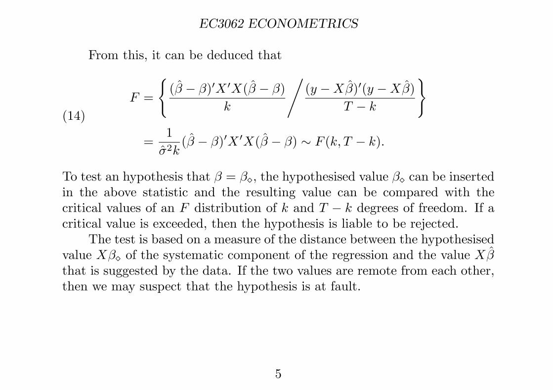
From this, it can be deduced that

(14)F =

{(β̂ − β)′X ′X(β̂ − β)

k

/(y − Xβ̂)′(y − Xβ̂)

T − k

}

=1

σ̂2k(β̂ − β)′X ′X(β̂ − β) ∼ F (k, T − k).

To test an hypothesis that β = β�, the hypothesised value β� can be insertedin the above statistic and the resulting value can be compared with thecritical values of an F distribution of k and T − k degrees of freedom. If acritical value is exceeded, then the hypothesis is liable to be rejected.

The test is based on a measure of the distance between the hypothesisedvalue Xβ� of the systematic component of the regression and the value Xβ̂that is suggested by the data. If the two values are remote from each other,then we may suspect that the hypothesis is at fault.

5

EC3062 ECONOMETRICS

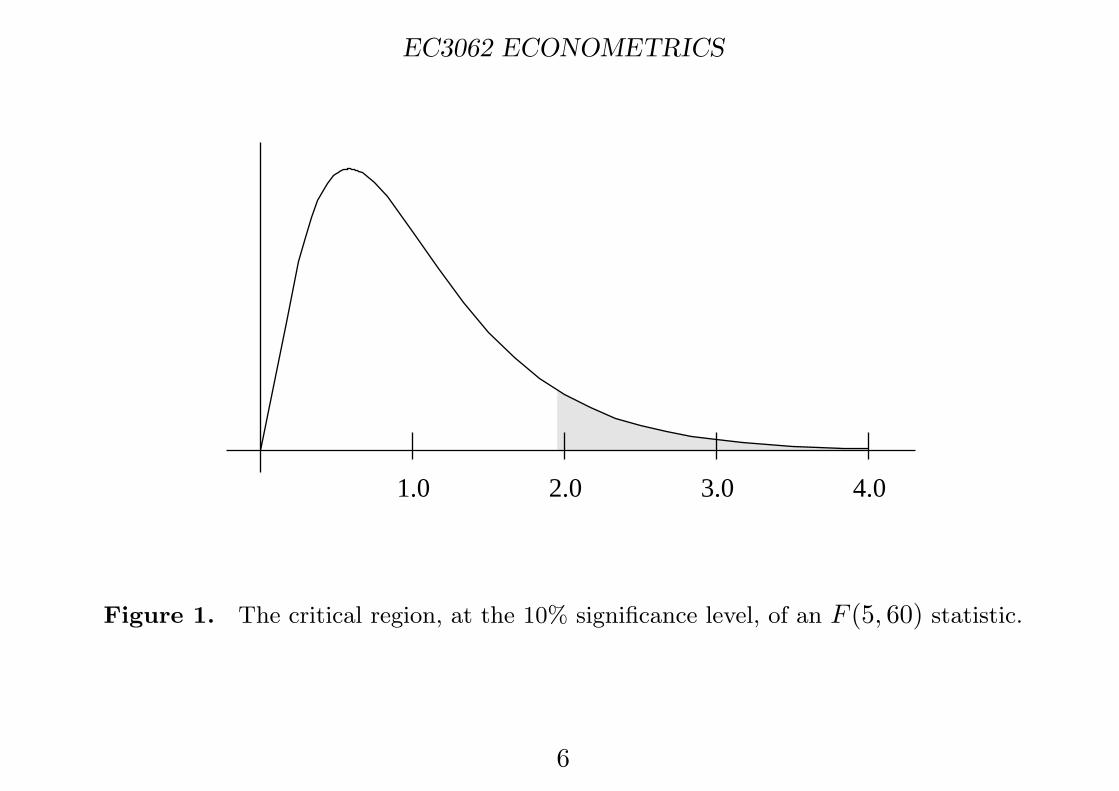
1.0 2.0 3.0 4.0

Figure 1. The critical region, at the 10% significance level, of an F (5, 60) statistic.

6

EC3062 ECONOMETRICS

To test an hypothesis that β2 = β2� in the model y = X1β1 + Xβ2 + εwhile ignoring β2, we use

(15) F =1

σ̂2k2(β̂2 − β2�)′X ′

2(I − P1)X2(β̂2 − β2�).

This will have an F (k2, T − k) distribution, if the hypothesis is true.By specialising the expression under (15), a statistic may be derived for

testing the hypothesis that βi = βi�, concerning a single element:

(16) F =(β̂i − βi�)2

σ̂2wii,

Here, wii stands for the ith diagonal element of (X ′X)−1. If the hypothesisis true, then this will have an F (1, T − k) distribution.

However, the usual way of testing such an hypothesis is to use

(17) t =β̂i − βi�√(σ̂2wii)

in conjunction with the tables of the t(T − k) distribution. The t statisticshows the direction in which the estimate of βi deviates from the hypothe-sised value as well as the size of the deviation.

7

EC3062 ECONOMETRICS

The Decomposition of a Chi-Square Variate: Cochrane’s Theorem

The standard test of an hypothesis regarding the vector β in the modelN(y;Xβ, σ2I) entails a multi-dimensional version of Pythagoras’ Theorem.Consider the decomposition of the vector y into the systematic componentand the residual vector. This gives

(18)y = Xβ̂ + (y − Xβ̂) and

y − Xβ = (Xβ̂ − Xβ) + (y − Xβ̂),

where the second equation comes from subtracting the unknown mean vectorXβ from both sides of the first. In terms of the projector P = X(X ′X)−1X ′,there is Xβ̂ = Py and e = y−Xβ̂ = (I −P )y. Also, ε = y−Xβ. Therefore,the two equations can be written as

(19)y = Py + (I − P )y and

ε = Pε + (I − P )ε.

8

EC3062 ECONOMETRICS

y

e

γ

Xβ^

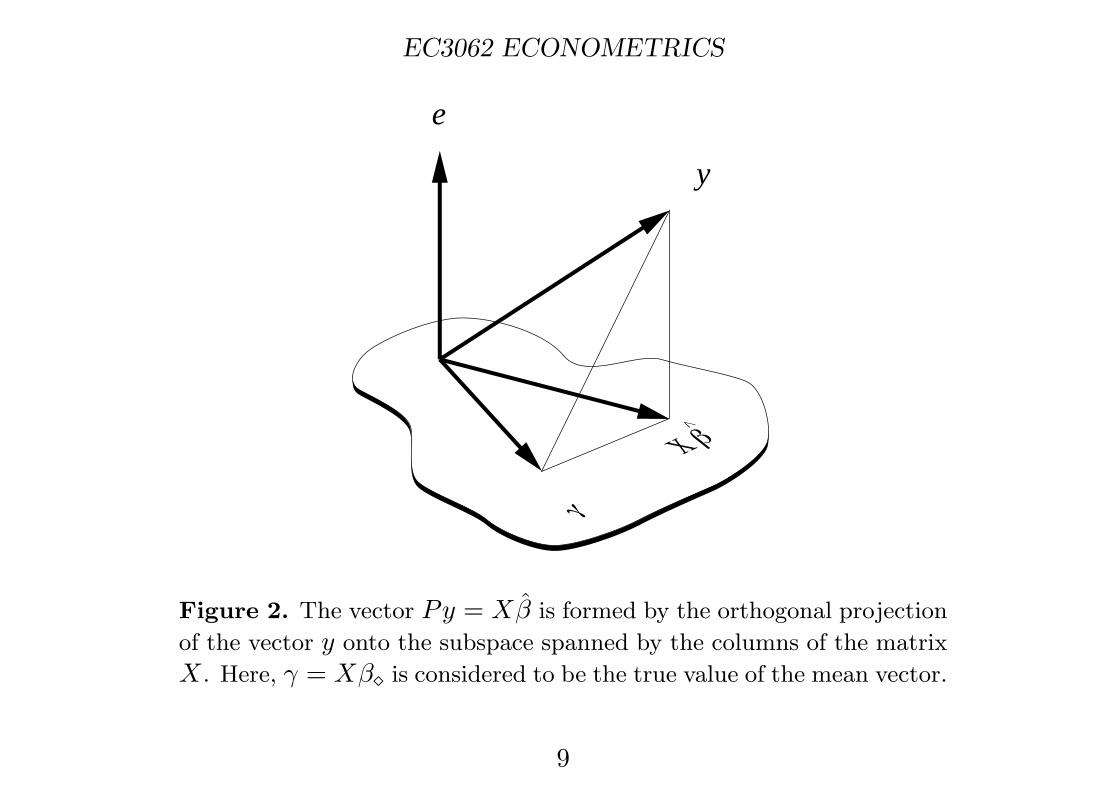
Figure 2. The vector Py = Xβ̂ is formed by the orthogonal projection

of the vector y onto the subspace spanned by the columns of the matrix

X . Here, γ = Xβ� is considered to be the true value of the mean vector.

9

EC3062 ECONOMETRICS

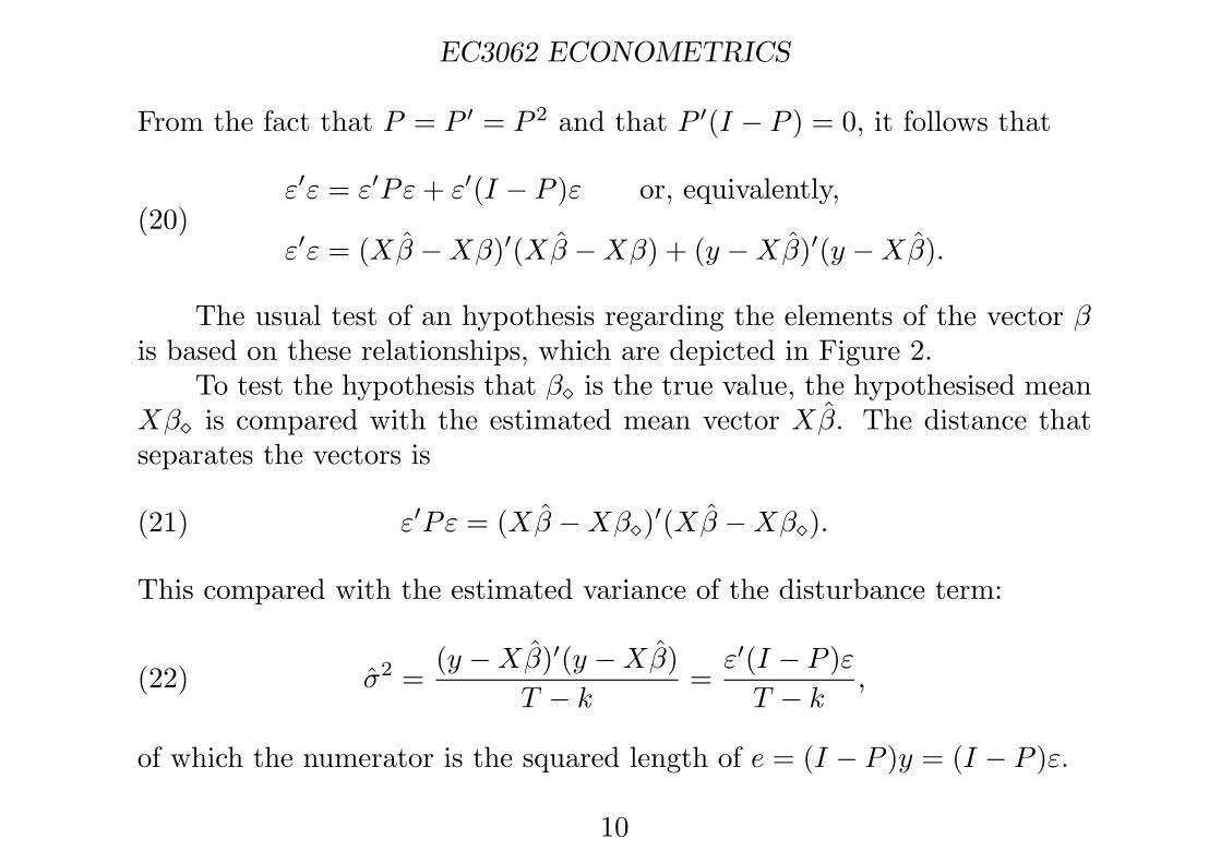
From the fact that P = P ′ = P 2 and that P ′(I − P ) = 0, it follows that

(20)ε′ε = ε′Pε + ε′(I − P )ε or, equivalently,

ε′ε = (Xβ̂ − Xβ)′(Xβ̂ − Xβ) + (y − Xβ̂)′(y − Xβ̂).

The usual test of an hypothesis regarding the elements of the vector βis based on these relationships, which are depicted in Figure 2.

To test the hypothesis that β� is the true value, the hypothesised meanXβ� is compared with the estimated mean vector Xβ̂. The distance thatseparates the vectors is

(21) ε′Pε = (Xβ̂ − Xβ�)′(Xβ̂ − Xβ�).

This compared with the estimated variance of the disturbance term:

(22) σ̂2 =(y − Xβ̂)′(y − Xβ̂)

T − k=

ε′(I − P )εT − k

,

of which the numerator is the squared length of e = (I − P )y = (I − P )ε.

10

EC3062 ECONOMETRICS

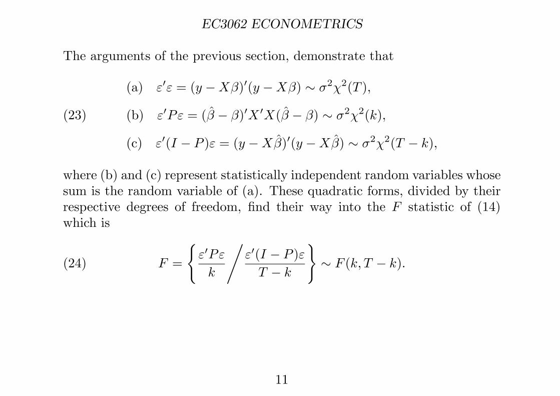
The arguments of the previous section, demonstrate that

(23)

(a) ε′ε = (y − Xβ)′(y − Xβ) ∼ σ2χ2(T ),

(b) ε′Pε = (β̂ − β)′X ′X(β̂ − β) ∼ σ2χ2(k),

(c) ε′(I − P )ε = (y − Xβ̂)′(y − Xβ̂) ∼ σ2χ2(T − k),

where (b) and (c) represent statistically independent random variables whosesum is the random variable of (a). These quadratic forms, divided by theirrespective degrees of freedom, find their way into the F statistic of (14)which is

(24) F =

{ε′Pε

k

/ε′(I − P )ε

T − k

}∼ F (k, T − k).

11

EC3062 ECONOMETRICS

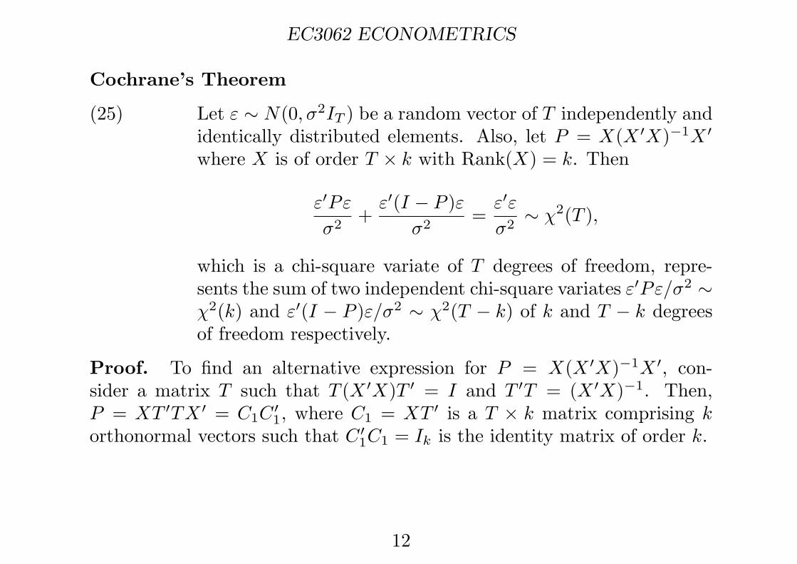
Cochrane’s Theorem

(25) Let ε ∼ N(0, σ2IT ) be a random vector of T independently andidentically distributed elements. Also, let P = X(X ′X)−1X ′

where X is of order T × k with Rank(X) = k. Then

ε′Pε

σ2+

ε′(I − P )εσ2

=ε′ε

σ2∼ χ2(T ),

which is a chi-square variate of T degrees of freedom, repre-sents the sum of two independent chi-square variates ε′Pε/σ2 ∼χ2(k) and ε′(I − P )ε/σ2 ∼ χ2(T − k) of k and T − k degreesof freedom respectively.

Proof. To find an alternative expression for P = X(X ′X)−1X ′, con-sider a matrix T such that T (X ′X)T ′ = I and T ′T = (X ′X)−1. Then,P = XT ′TX ′ = C1C

′1, where C1 = XT ′ is a T × k matrix comprising k

orthonormal vectors such that C ′1C1 = Ik is the identity matrix of order k.

12

EC3062 ECONOMETRICS

Now define C2 to be a complementary matrix of T − k orthonormalvectors. Then, C = [C1, C2] is an orthonormal matrix of order T such that

(26)

CC ′ = C1C′1 + C2C

′2 = IT and

C ′C =[

C ′1C1 C ′

1C2

C ′2C1 C ′

2C2

]=

[Ik 00 IT−k

].

The first of these results allows us to set I − P = I − C1C′1 = C2C

′2. Now,

if ε ∼ N(0, σ2IT ) and if C is an orthonormal matrix such that C ′C = IT ,then it follows that C ′ε ∼ N(0, σ2IT ). On partitioning C ′ε, we find that

(27)[

C ′1ε

C ′2ε

]∼ N

([00

],

[σ2Ik 0

0 σ2IT−k

]),

which is to say that C ′1ε ∼ N(0, σ2Ik) and C ′

2ε ∼ N(0, σ2IT−k) are indepen-dently distributed normal vectors.

13

EC3062 ECONOMETRICS

It follows that

(28)

ε′C1C′1ε

σ2=

ε′Pε

σ2∼ χ2(k) and

ε′C2C′2ε

σ2=

ε′(I − P )εσ2

∼ χ2(T − k)

are independent chi-square variates. Since C1C′1 + C2C

′2 = IT , the sum of

these two variates is

(29)ε′C1C

′1ε

σ2+

ε′C2C′2ε

σ2=

ε′ε

σ2∼ χ2(T );

and thus the theorem is proved.The statistic under (14) can now be expressed in the form of

(30) F =

{ε′Pε

k

/ε′(I − P )ε

T − k

}.

This is manifestly the ratio of two chi-square variates divided by their respec-tive degrees of freedom; and so it has an F distribution with these degreesof freedom. This result provides the means for testing the hypothesis con-cerning the parameter vector β.

14

EC3062 ECONOMETRICS

Hypotheses Concerning Subsets of the Regression Coefficients

Consider the restrictions Rβ = r on the regression coefficients of themodel N(y;Xβ, σ2I), where R is a j × k matrix rank j. Given that β̂ ∼N{β, σ2(X ′X)−1}, it follows that

(32) Rβ̂ ∼ N{Rβ = r, σ2R(X ′X)−1R′};

and, from this, it can be inferred immediately that

(33)(Rβ̂ − r)′

{R(X ′X)−1R′}−1(Rβ̂ − r)

σ2∼ χ2(j).

Since, it is statistically independent of β̂,

(34)(T − k)σ̂2

σ2=

(y − Xβ̂)′(y − Xβ̂)σ2

∼ χ2(T − k)

must be statistically independent of the chi-square variate of (33).

15

EC3062 ECONOMETRICS

Therefore, it can be deduced that

(36)

F =

{(Rβ̂ − r)′

{R(X ′X)−1R′}−1(Rβ̂ − r)

j

/(y − Xβ̂)′(y − Xβ̂)

T − k

}

=(Rβ̂ − r)′

{R(X ′X)−1R′}−1(Rβ̂ − r)

σ̂2j∼ F (j, T − k),

This F statistic can be used in testing the validity of the hypothesisedrestrictions Rβ = r.

Let β′ = [β′1, β

′2]

′. Then, the condition that the subvector β1 assumesthe value of β�

1 can be expressed via the equation

(37) [Ik1 , 0][

β1

β2

]= β�

1 .

This can be construed as a case of the equation Rβ = r, where R = [Ik1 , 0]and r = β�

1 .

16

EC3062 ECONOMETRICS

The partitioned form of (X ′X)−1 is

(X ′X)−1 =[

X ′1X1 X ′

1X2

X ′2X1 X ′

2X2

]−1

=

[{X ′

1(I − P2)X1}−1 − {X ′1(I − P2)X1}−1X ′

1X2(X ′2X2)−1

−{X ′2(I − P1)X2}−1X ′

2X1(X ′1X1)−1 {X ′

2(I − P1)X2}−1

].

With R = [I, 0], we find that

(39) R(X ′X)−1R′ ={X ′

1(I − P2)X1

}−1.

Therefore, for testing the hypothesis that β1 = β�1 , we use

(40)

F =

{(β̂1 − β�

1)′{X ′

1(I − P2)X1

}(β̂1 − β�

1)k1

/(y − Xβ̂)′(y − Xβ̂)

T − k

}

=(β̂1 − β�

1)′{X ′

1(I − P2)X ′1

}(β̂1 − β�

1)σ̂2k1

∼ F (k1, T − k).

17

EC3062 ECONOMETRICS

Finally, for the jth element of β̂, there is

(41)(β̂j − βj)2/σ2wjj ∼ F (1, T − k) or, equivalently,

(β̂j − βj)√

σ2wjj ∼ t(T − k),

where wjj is the jth diagonal element of (X ′X)−1 and t(T − k) denotes thet distribution of T − k degrees of freedom.

18

EC3062 ECONOMETRICS

An Alternative Formulation of the F statistic

An alternative way of forming the F statistic uses the products of twoseparate regressions. Consider the formula for the restricted least-squaresestimator that has been given under (2.76):

(42) β∗ = β̂ − (X ′X)−1R′{R(X ′X)−1R′}−1(Rβ̂ − r).

From this, the following expression for the residual sum of squares of therestricted regression is is derived:

(43) y − Xβ∗ = (y − Xβ̂) + X(X ′X)−1R′{R(X ′X)−1R′}−1(Rβ̂ − r).

The two terms on the RHS are mutually orthogonal on account of the condi-tion (y−Xβ̂)′X = 0. Therefore, the residual sum of squares of the restrictedregression is

(44)(y − Xβ∗)′(y − Xβ∗) = (y − Xβ̂)′(y − Xβ̂) +

(Rβ̂ − r)′{R(X ′X)−1R′}−1(Rβ̂ − r).

19

EC3062 ECONOMETRICS

This equation can be rewritten as

(45) RSS − USS = (Rβ̂ − r)′{R(X ′X)−1R′}−1(Rβ̂ − r),

where RSS denotes the restricted sum of squares an USS denotes the un-restricted sum of squares. It follows that the test statistic of (36) can bewritten as

(46) F =

{RSS − USS

j

/USS

T − k

}.

This formulation can be used, for example, in testing the restrictionthat β1 = 0 in the partitioned model N(y;X1β1 + X2β2, σ

2I). Then, interms of equation (37), there is R = [Ik1 , 0] and there is r = β�

1 = 0, whichgives

(47)RSS − USS = β̂′

1X′1(I − P2)X1β̂1

= y′(I − P2)X1{X ′1(I − P2)X1}−1X ′

1(I − P2)y.

20

EC3062 ECONOMETRICS

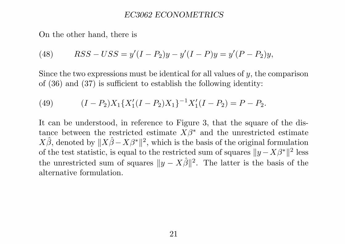
On the other hand, there is

(48) RSS − USS = y′(I − P2)y − y′(I − P )y = y′(P − P2)y,

Since the two expressions must be identical for all values of y, the comparisonof (36) and (37) is sufficient to establish the following identity:

(49) (I − P2)X1{X ′1(I − P2)X1}−1X ′

1(I − P2) = P − P2.

It can be understood, in reference to Figure 3, that the square of the dis-tance between the restricted estimate Xβ∗ and the unrestricted estimateXβ̂, denoted by ‖Xβ̂−Xβ∗‖2, which is the basis of the original formulationof the test statistic, is equal to the restricted sum of squares ‖y−Xβ∗‖2 lessthe unrestricted sum of squares ‖y − Xβ̂‖2. The latter is the basis of thealternative formulation.

21

EC3062 ECONOMETRICS

Xβ*

Xβ^

y

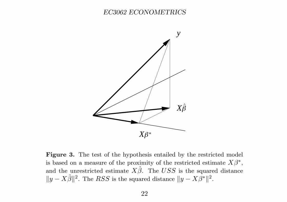
Figure 3. The test of the hypothesis entailed by the restricted model

is based on a measure of the proximity of the restricted estimate Xβ∗,and the unrestricted estimate Xβ̂. The USS is the squared distance

‖y − Xβ̂‖2. The RSS is the squared distance ‖y − Xβ∗‖2.

22