Deterministic Scheduling - UAB Barcelonamat.uab.cat/~alseda/MasterOpt/orv2.pdf · Krzysztof Giaro...
101
Deterministic Scheduling Dr inż. Krzysztof Giaro Gdańsk University of Technology
Transcript of Deterministic Scheduling - UAB Barcelonamat.uab.cat/~alseda/MasterOpt/orv2.pdf · Krzysztof Giaro...
Deterministic Scheduling
Dr inż. Krzysztof Giaro
Gdańsk University of Technology
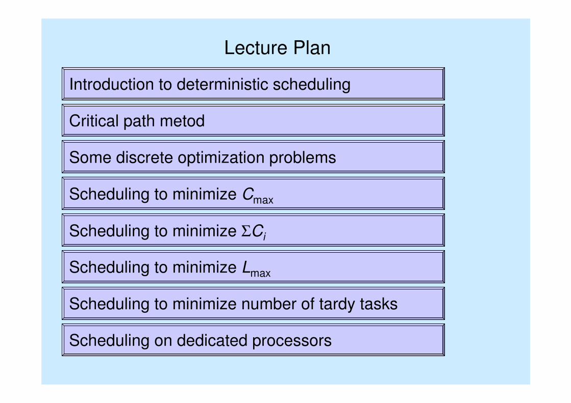
Lecture Plan
Introduction to deterministic scheduling
Critical path metod
Scheduling to minimize Cmax
Scheduling to minimize ΣCi
Scheduling to minimize Lmax
Scheduling on dedicated processors
Some discrete optimization problems
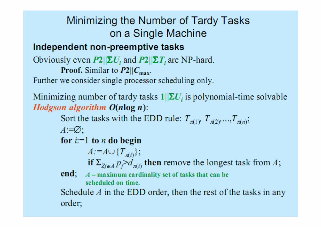
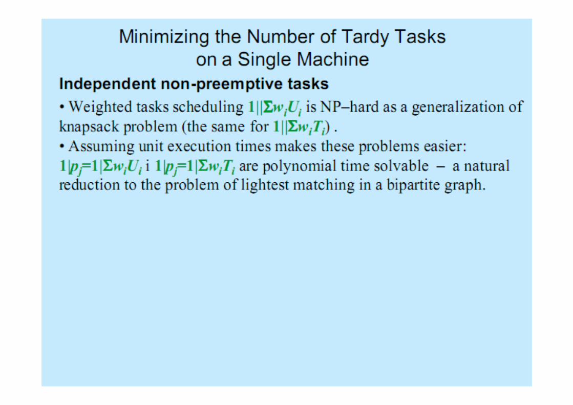
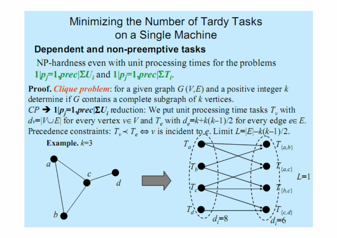
Scheduling to minimize number of tardy tasks
Introduction to Deterministic Scheduling
Our aim is to schedule the given set of tasks (programs etc.) on
machines (or processors).
We have to construct a schedule that fulfils given constraints andminimizes optimality criterion (objective function).
Deterministic model: all the parameters of the system and of the tasks
are known in advance.
Genesis and practical motivations:
• scheduling manufacturing processes,
• project planning,
• school or conference timetabling,
• scheduling tasks in multitask operating systems,
• distributed computing.
Introduction to Deterministic Scheduling
M1
M2
M3
J 2
9
J 4J 1
J 5J 3
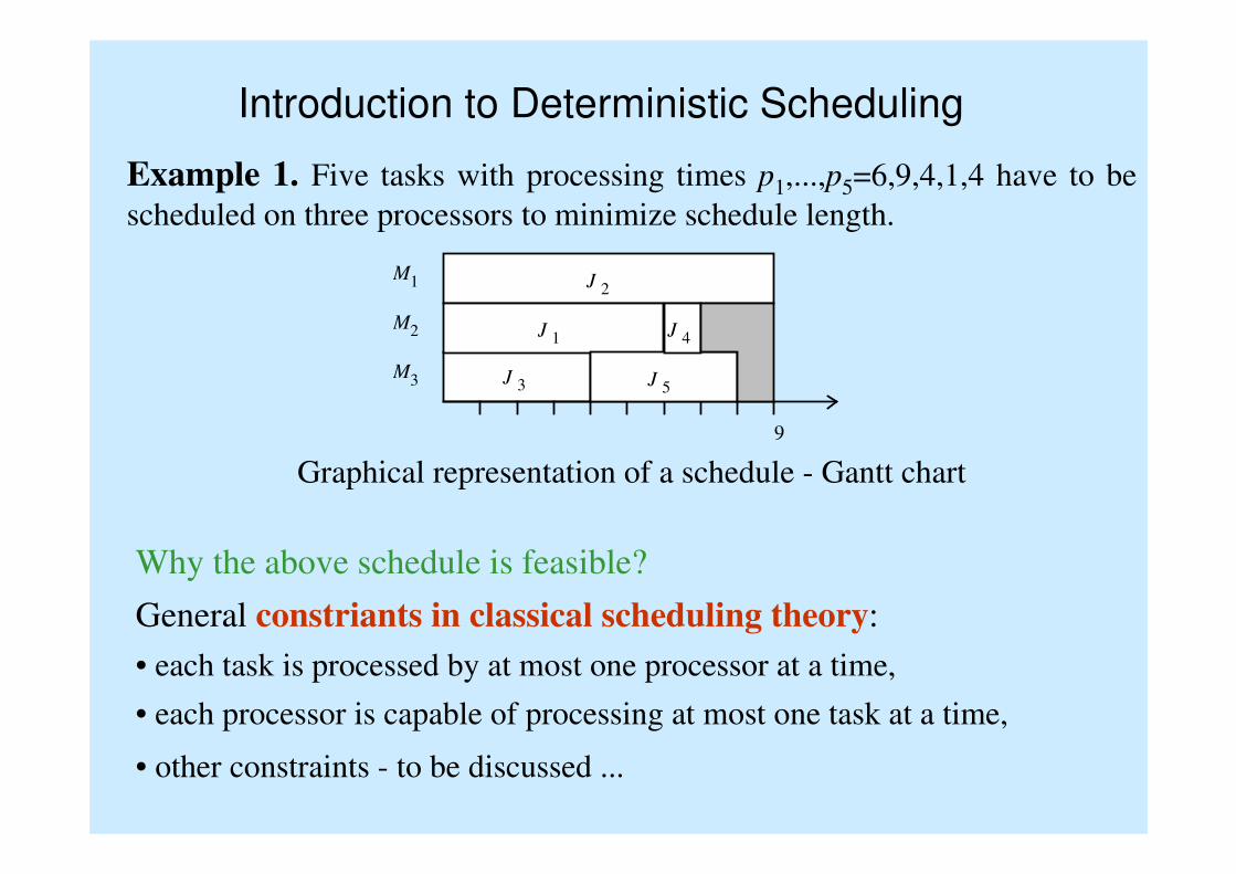
Graphical representation of a schedule - Gantt chart
Example 1. Five tasks with processing times p1,...,p5=6,9,4,1,4 have to be
scheduled on three processors to minimize schedule length.
Why the above schedule is feasible?
General constriants in classical scheduling theory:
• each task is processed by at most one processor at a time,
• each processor is capable of processing at most one task at a time,
• other constraints - to be discussed ...
Introduction to Deterministic Scheduling
Processors characterization
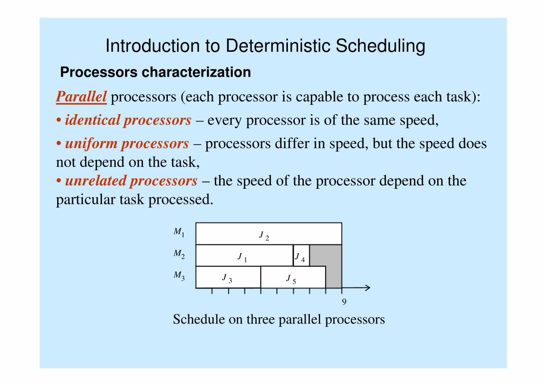
Parallel processors (each processor is capable to process each task):
• identical processors – every processor is of the same speed,
• uniform processors – processors differ in speed, but the speed does
not depend on the task,
• unrelated processors – the speed of the processor depend on the
particular task processed.
M1
M2
M3
J 2
9
J 4J 1
J 5J 3
Schedule on three parallel processors
Introduction to Deterministic SchedulingProcessors characterization
Dedicated processors
• Each job consists of the set of tasks preassigned to processors (job Jj
consists of tasks Tij preassigned to Mi, of processing time pij). The job is
completed at the time the latest task is completed,
• some jobs may not need all the processors (empty operations),
• no two tasks of the same job can be scheduled in parallel,
• a processor is capable to process at most one task at a time.
There are three models of scheduling on dedicated processors:
• flow shop – all jobs have the same processing order through the machines
coincident with machine numbering,
• open shop – the sequenice of tasks within each job is arbitrary,
• job shop – the machine sequence of each job is given and may differ
between jobs.
Introduction to Deterministic Scheduling
Processors characterization
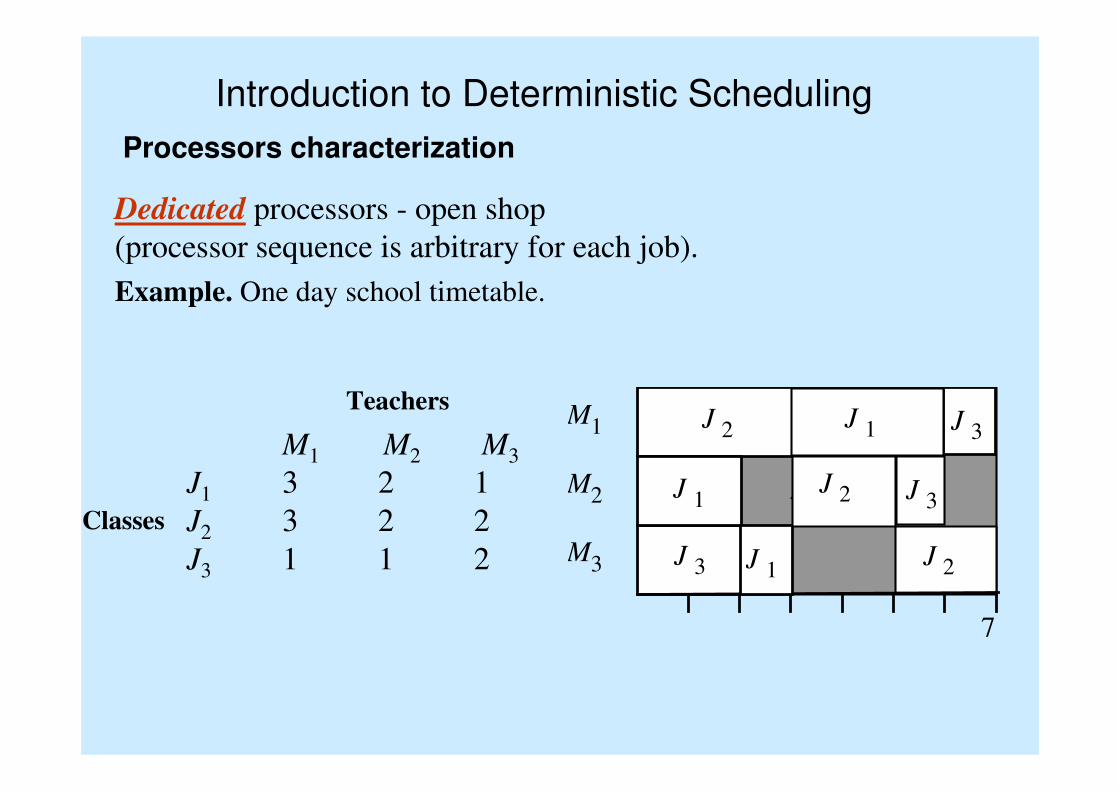
Dedicated processors - open shop
(processor sequence is arbitrary for each job).
M1
M2
M3
J 2
7
J 3
Z 1J 1
J 2
J 2
J 1
J 1J 3
J 3
Teachers
Classes
M1 M2 M3
J1 3 2 1
J2 3 2 2
J3 1 1 2
Example. One day school timetable.
Introduction to Deterministic Scheduling
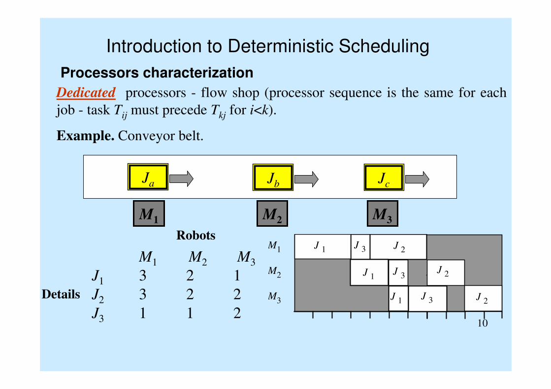
Processors characterization
Dedicated processors - flow shop (processor sequence is the same for each
job - task Tij must precede Tkj for i<k).
M1
M2
M3
J 2
10
J 3
J 1 Z 1J 2
J 2
J 1
J 1 J 3
J 3
Robots
Details
M1 M2 M3
J1 3 2 1
J2 3 2 2
J3 1 1 2
Ja Jb Jc
M1 M2 M3
Example. Conveyor belt.
Introduction to Deterministic Scheduling
Processors characterization
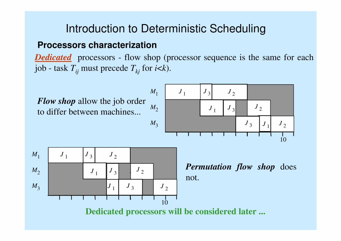
Dedicated processors - flow shop (processor sequence is the same for each
job - task Tij must precede Tkj for i<k).
M1
M2
M3
J 2
10
J 3
J 1 Z1J 2
J 2
J 1
J 1J 3
J 3
M1
M2
M3
J 2
10
J 3
J 1 Z 1J 2
J 2
J 1
J 1 J 3
J 3
Flow shop allow the job order
to differ between machines...
Permutation flow shop does
not.
Dedicated processors will be considered later ...
Introduction to Deterministic Scheduling
Tasks characterization
Task Tj :
• Processing time. It is independent of processor in case of identical
processors and is denoted pj. In the case of uniform processors,
processor Mi speed is denoted bi, and the processing time of Tj on Mi is
pj/bi. In the case of unrelated processors the processing time of Tj on Mi
is pij.
• Release (or arrival) time rj. The time at which the task is ready for
processing. By default all release times are zero.
• Due date dj. Specifies the time limit by which should be completed.
Usually, penalty functions are defined in accordance with due dates, or
dj denotes the ‘hard’ time limit (deadline) by which Tj must be
completed (exact meaning comes from the context).
• Weight wj – expresses the relative urgency of Tj, by default wj=1.
There are given: the set of n tasks T={T1,...,Tn} and m machines
(processors) M={M1,...,Mm}.
Introduction to Deterministic Scheduling
Tasks characterization
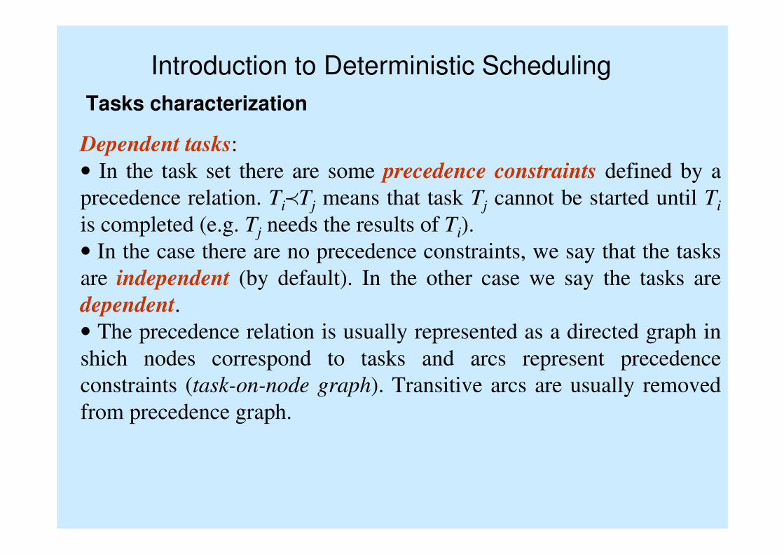
Dependent tasks:
• In the task set there are some precedence constraints defined by a
precedence relation. TipTj means that task Tj cannot be started until Ti
is completed (e.g. Tj needs the results of Ti).
• In the case there are no precedence constraints, we say that the tasks
are independent (by default). In the other case we say the tasks are
dependent.
• The precedence relation is usually represented as a directed graph in
shich nodes correspond to tasks and arcs represent precedence
constraints (task-on-node graph). Transitive arcs are usually removed
from precedence graph.
Introduction to Deterministic Scheduling
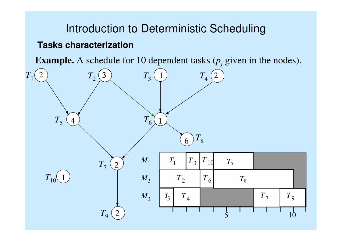
Tasks characterization
Example. A schedule for 10 dependent tasks (pj given in the nodes).
2
6
4T5 1
1
2 3 1T1 T2 T3 T4
T6
T7
T8
T9
T10
2
2
M1
M2
M3
T 2
10
T 10 T5
Z 1T9T 4
T1 T 3
T3
T 6
5
Z 1T 7
T8
2
4 1
1
2 3 1 2
2
Introduction to Deterministic Scheduling
Tasks characterization
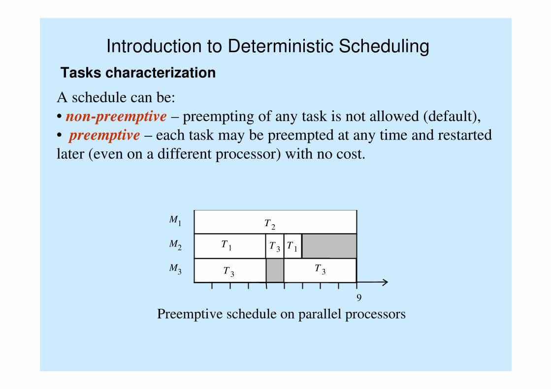
A schedule can be:
• non-preemptive – preempting of any task is not allowed (default),
• preemptive – each task may be preempted at any time and restarted
later (even on a different processor) with no cost.
Preemptive schedule on parallel processors
M1
M2
M3
T 2
9
T 1T 1
T 3
T 3
T 3
Introduction to Deterministic Scheduling
Feasible schedule conditions (gathered):
• each processor is assigned to at most one task at a time,
• each task is processed by at most one machine at a time,
• task Tj is processed completly in the time interval [rj,∞) (or
within [rj, dj), when deadlines are present),
• precedence constraints are satisfied,
• in the case of non-preemptive scheduling no task is
preempted, otherwise the number of preemptions is finite.
Introduction to Deterministic Scheduling
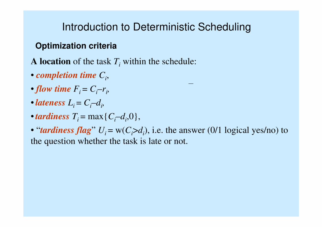
A location of the task Ti within the schedule:
• completion time Ci,
• flow time Fi = Ci–ri,
• lateness Li = Ci–di,
• tardiness Ti = max{Ci–di,0},
• “tardiness flag” Ui = w(Ci>di), i.e. the answer (0/1 logical yes/no) to
the question whether the task is late or not.
Optimization criteria
Introduction to Deterministic Scheduling
Optimization criteria
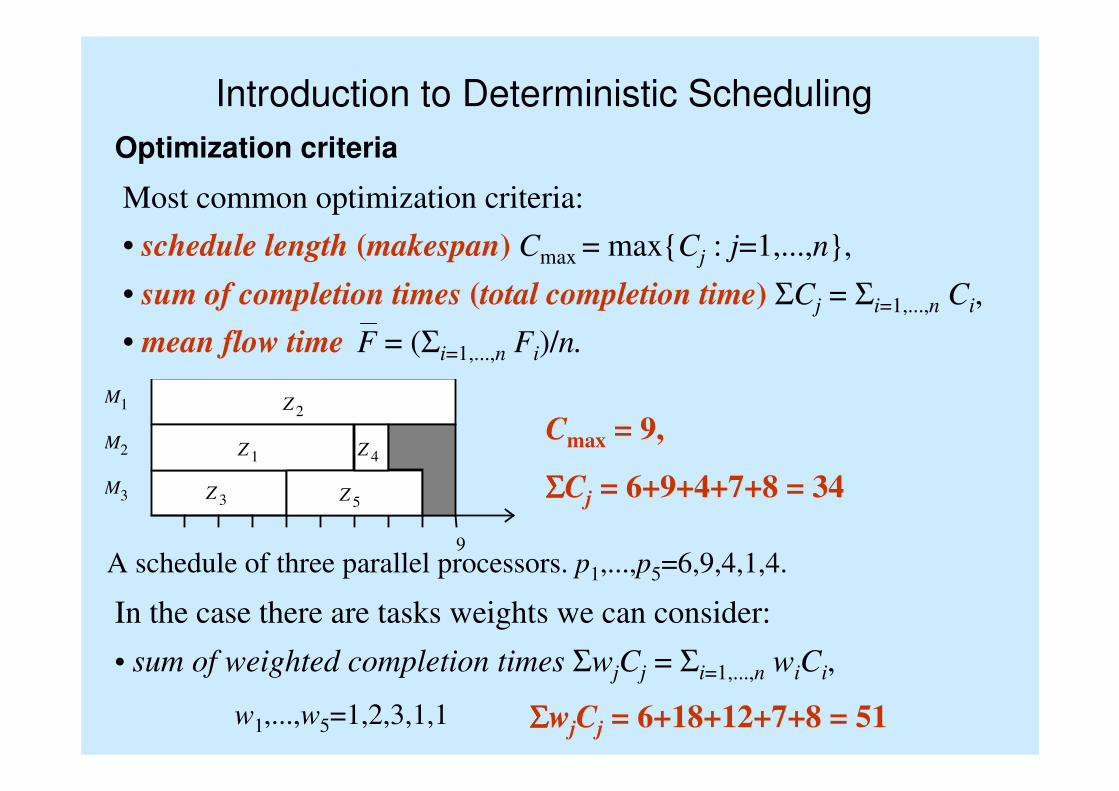
Most common optimization criteria:
• schedule length (makespan) Cmax = max{Cj : j=1,...,n},
• sum of completion times (total completion time) ΣCj = Σi=1,...,n Ci,
• mean flow time F = (Σi=1,...,n Fi)/n.
M1
M2
M3
Z 2
9
Z 4Z 1
Z 5Z 3
A schedule of three parallel processors. p1,...,p5=6,9,4,1,4.
Cmax = 9,
ΣΣΣΣCj = 6+9+4+7+8 = 34
In the case there are tasks weights we can consider:
• sum of weighted completion times ΣwjCj = Σi=1,...,n wiCi,
w1,...,w5=1,2,3,1,1 ΣΣΣΣwjCj = 6+18+12+7+8 = 51
Introduction to Deterministic Scheduling
Optimization criteria
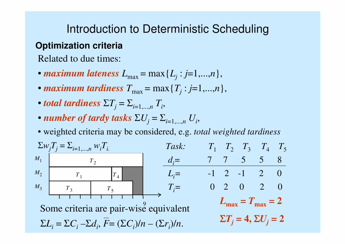
Related to due times:
• maximum lateness Lmax = max{Lj : j=1,...,n},
• maximum tardiness Tmax = max{Tj : j=1,...,n},
• total tardiness ΣTj = Σi=1,...,n Ti,
• number of tardy tasks ΣUj = Σi=1,...,n Ui,
• weighted criteria may be considered, e.g. total weighted tardiness
ΣwjTj = Σi=1,...,n wiTi.
M1
M2
M3
T 2
9
T 4T 1
T
Z5
T 3
Lmax = Tmax = 2
ΣΣΣΣTj = 4, ΣΣΣΣUj = 2
Li= -1 2 -1 2 0
Ti= 0 2 0 2 0
Task: T1 T2 T3 T4 T5
di= 7 7 5 5 8
Some criteria are pair-wise equivalent
ΣLi = ΣCi –Σdi, F= (ΣCi)/n – (Σri)/n.
Introduction to Deterministic Scheduling
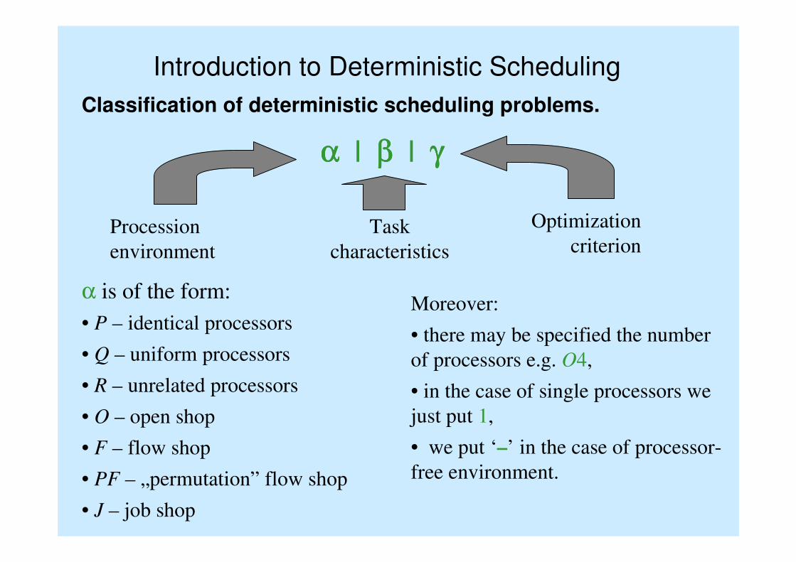
Classification of deterministic scheduling problems.
αααα | ββββ | γγγγ
Procession
environment
Task
characteristics
Optimization
criterion
α is of the form:
• P – identical processors
• Q – uniform processors
• R – unrelated processors
• O – open shop
• F – flow shop
• PF – „permutation” flow shop
• J – job shop
Moreover:
• there may be specified the number
of processors e.g. O4,
• in the case of single processors we
just put 1,
• we put ‘–’ in the case of processor-
free environment.
Introduction to Deterministic Scheduling
Classification of deterministic scheduling problems.
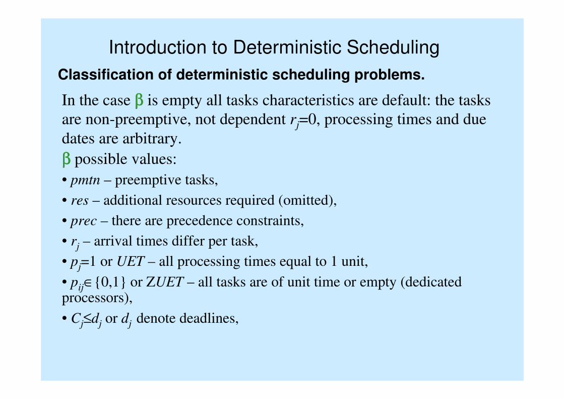
ββββ possible values:
• pmtn – preemptive tasks,
• res – additional resources required (omitted),
• prec – there are precedence constraints,
• rj – arrival times differ per task,
• pj=1 or UET – all processing times equal to 1 unit,
• pij∈{0,1} or ZUET – all tasks are of unit time or empty (dedicatedprocessors),
• Cj≤dj or dj denote deadlines,
In the case ββββ is empty all tasks characteristics are default: the tasks
are non-preemptive, not dependent rj=0, processing times and due
dates are arbitrary.
Introduction to Deterministic Scheduling
Classification of deterministic scheduling problems.
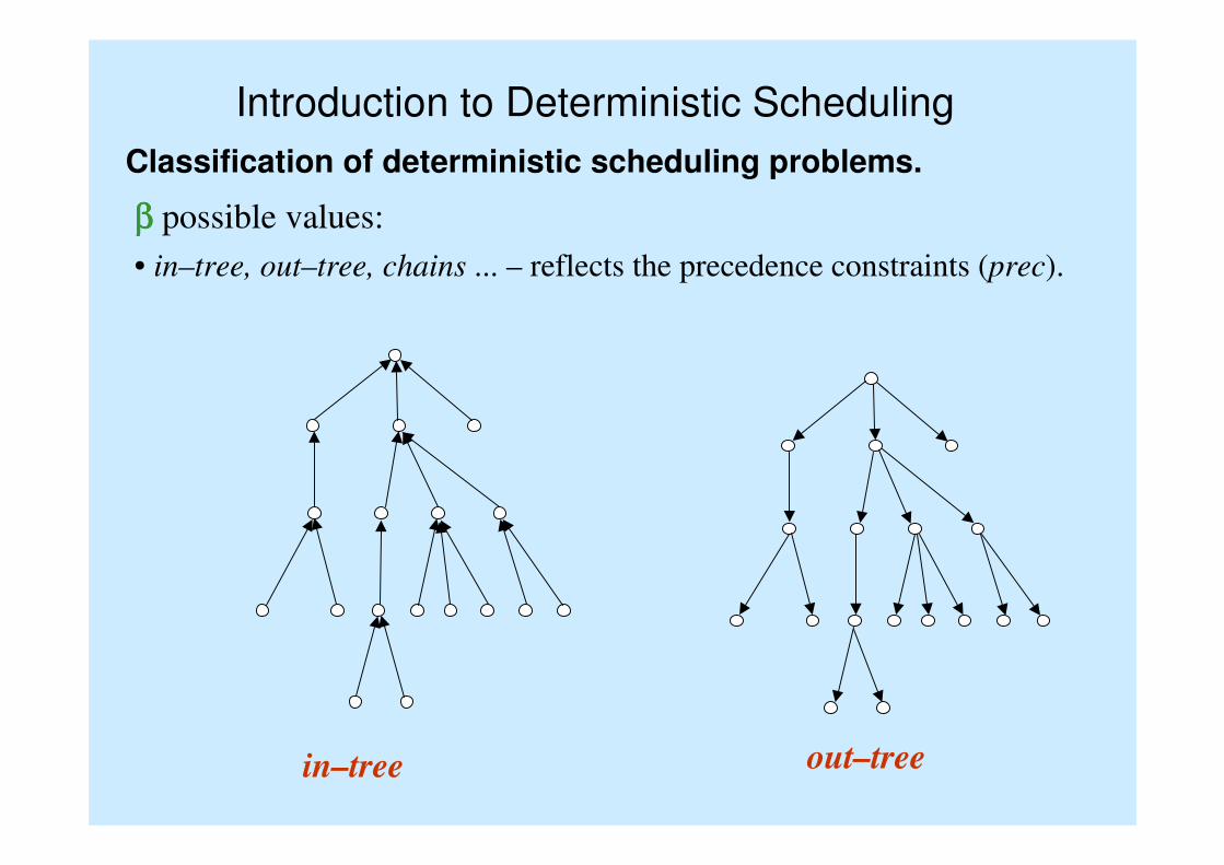
ββββ possible values:
• in–tree, out–tree, chains ... – reflects the precedence constraints (prec).
out–treein–tree
Introduction to Deterministic Scheduling
Classification of deterministic scheduling problems.
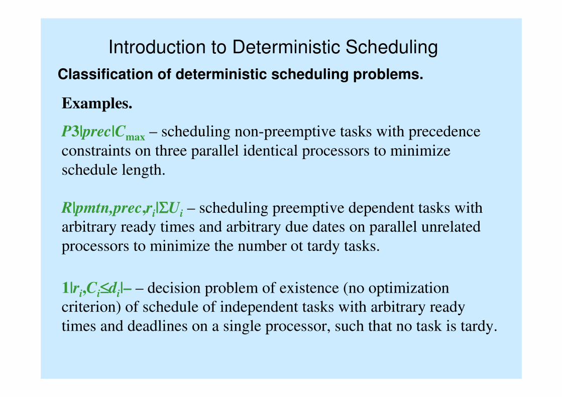
Examples.
P3|prec|Cmax – scheduling non-preemptive tasks with precedence
constraints on three parallel identical processors to minimize
schedule length.
R|pmtn,prec,ri|ΣΣΣΣUi – scheduling preemptive dependent tasks with
arbitrary ready times and arbitrary due dates on parallel unrelated
processors to minimize the number ot tardy tasks.
1|ri,Ci≤≤≤≤di|– – decision problem of existence (no optimization
criterion) of schedule of independent tasks with arbitrary ready
times and deadlines on a single processor, such that no task is tardy.
Introduction to Deterministic Scheduling
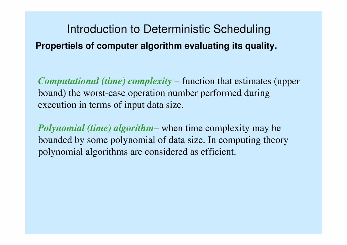
Propertiels of computer algorithm evaluating its quality.
Computational (time) complexity – function that estimates (upper
bound) the worst-case operation number performed during
execution in terms of input data size.
Polynomial (time) algorithm– when time complexity may be
bounded by some polynomial of data size. In computing theory
polynomial algorithms are considered as efficient.
Introduction to Deterministic Scheduling
Propertiels of computer algorithm evaluating its quality.
NP-hard problems – are commonly believed not to have
polynomial time algorithms solving them. For these problems we
can only use fast but not accurate procedures or (for small
instances) long time heuristics. NP-hardness is treated as
computational intractability.
How to prove that problem A is NP-hard?
Sketch: Find any NP-hard problem B and show the efficient
(polynomial) procedure that reduces (translates) B into A. Then A is
not less general problem than B, therefore if B was hard, so is A.
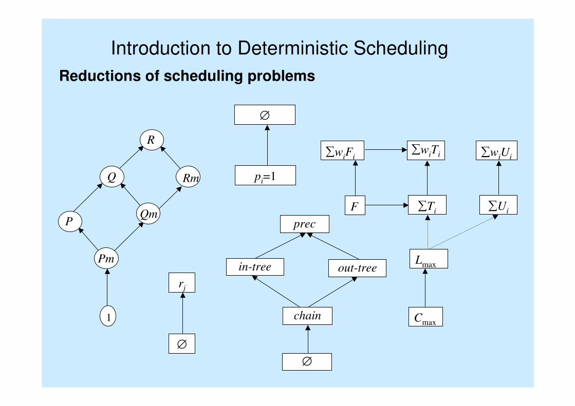
Introduction to Deterministic Scheduling
Reductions of scheduling problems
1
P
Pm
Q
Qm
R
Rm
∅
pi=1
∅
rj
∑wiFi
F
∑wiTi
∑Ti
∑wiUi
∑Ui
Lmax
Cmax
prec
chain
∅
out-treein-tree
Introduction to Deterministic Scheduling
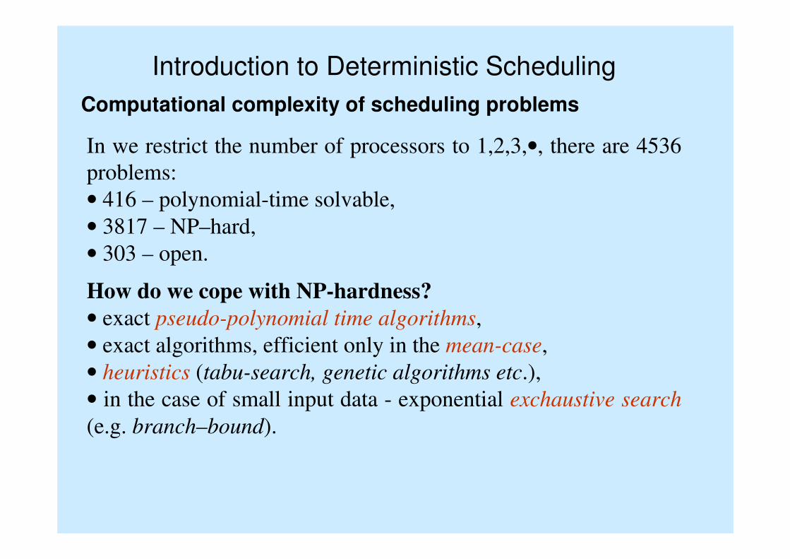
Computational complexity of scheduling problems
In we restrict the number of processors to 1,2,3,•, there are 4536
problems:
• 416 – polynomial-time solvable,
• 3817 – NP–hard,
• 303 – open.
How do we cope with NP-hardness?
• exact pseudo-polynomial time algorithms,
• exact algorithms, efficient only in the mean-case,
• heuristics (tabu-search, genetic algorithms etc.),
• in the case of small input data - exponential exchaustive search
(e.g. branch–bound).
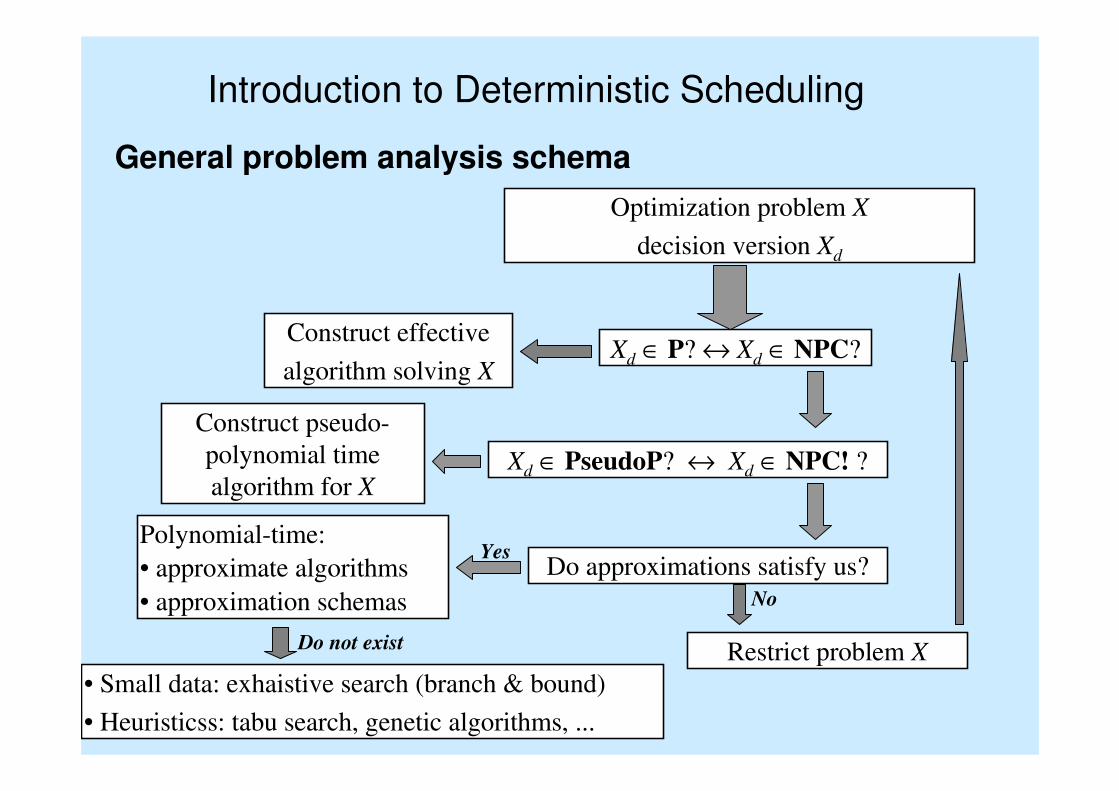
General problem analysis schema
Optimization problem X
decision version Xd
Xd ∈ P? ↔ Xd ∈ NPC?Construct effective
algorithm solving X
Xd ∈ PseudoP? ↔ Xd ∈ NPC! ?
Construct pseudo-
polynomial time
algorithm for X
Do approximations satisfy us?Yes
Polynomial-time:
• approximate algorithms
• approximation schemas No
Restrict problem X
• Small data: exhaistive search (branch & bound)
• Heuristicss: tabu search, genetic algorithms, ...
Do not exist
Introduction to Deterministic Scheduling
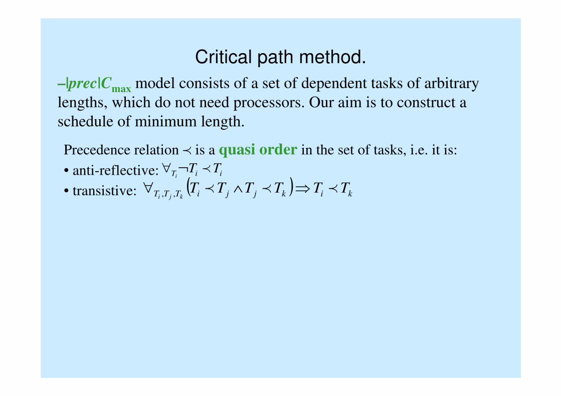
Critical path method.
–|prec|Cmax model consists of a set of dependent tasks of arbitrary
lengths, which do not need processors. Our aim is to construct a
schedule of minimum length.
Precedence relation p is a quasi order in the set of tasks, i.e. it is:
• anti-reflective:
• transistive:
iiT TTi
p¬∀
( )kikjjiTTT TTTTTT
kjippp ⇒∧∀ ,,
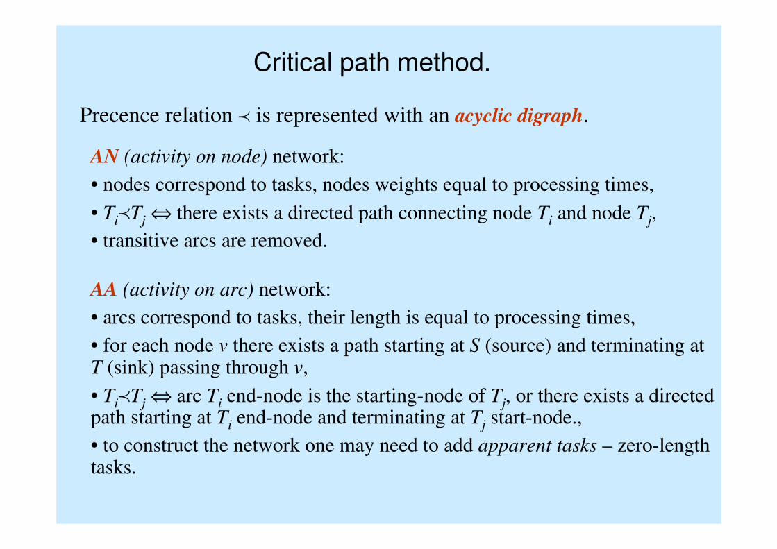
Critical path method.
Precence relation p is represented with an acyclic digraph.
AN (activity on node) network:
• nodes correspond to tasks, nodes weights equal to processing times,
• TipTj ⇔ there exists a directed path connecting node Ti and node Tj,
• transitive arcs are removed.
AA (activity on arc) network:
• arcs correspond to tasks, their length is equal to processing times,
• for each node v there exists a path starting at S (source) and terminating atT (sink) passing through v,
• TipTj ⇔ arc Ti end-node is the starting-node of Tj, or there exists a directedpath starting at Ti end-node and terminating at Tj start-node.,
• to construct the network one may need to add apparent tasks – zero-lengthtasks.
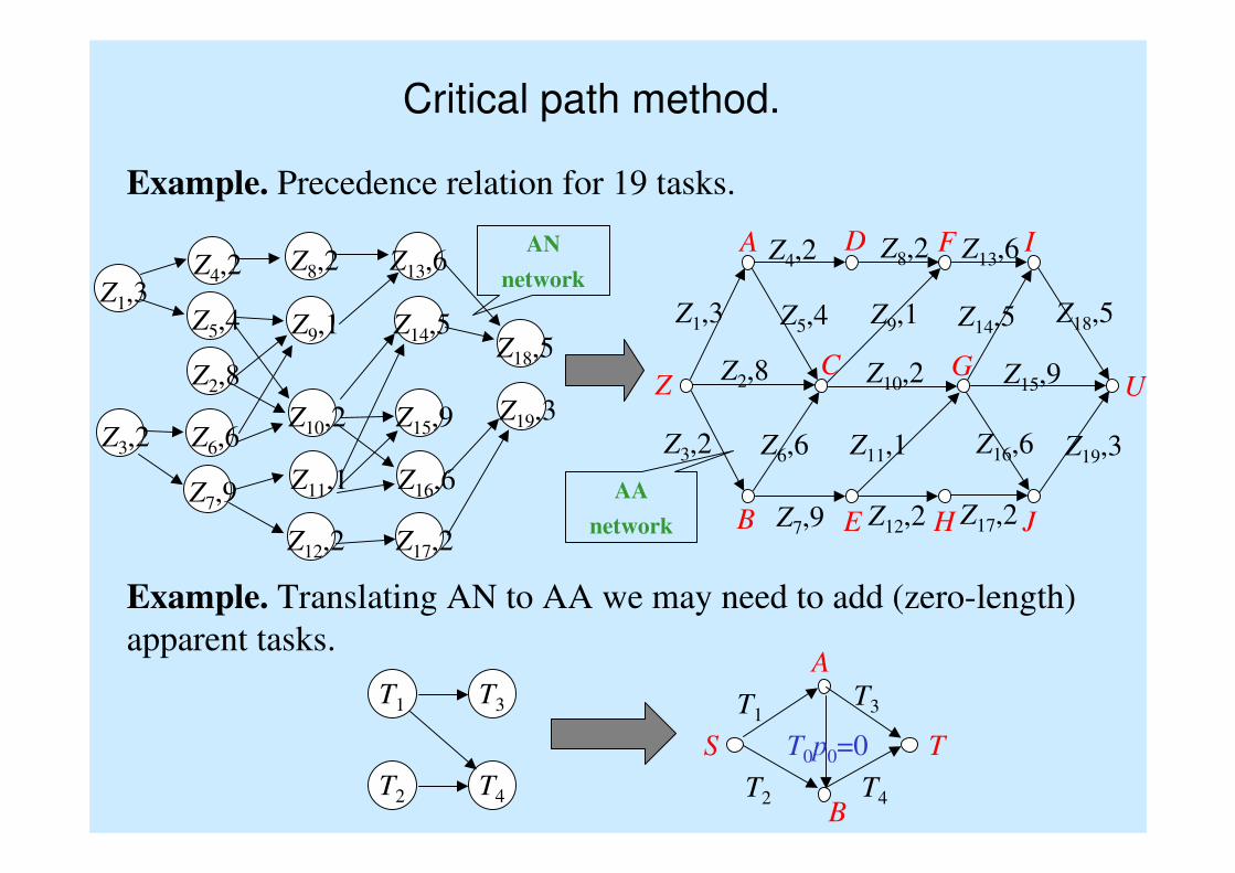
Critical path method.
Example. Precedence relation for 19 tasks.
Z1,3
Z2,8
Z3,2
Z4,2
Z5,4
Z6,6
Z7,9
Z9,1
Z10,2
Z8,2
Z11,1
Z12,2
Z14,5
Z15,9
Z13,6
Z16,6
Z17,2
Z18,5
Z19,3
AN
network
A
ZC G
U
B E H J
D F I
Z19,3
Z13,6Z8,2Z4,2
Z2,8 Z10,2 Z15,9
Z17,2Z12,2Z7,9
Z18,5Z14,5Z9,1Z5,4Z1,3
Z3,2 Z6,6 Z11,1 Z16,6
AA
network
Example. Translating AN to AA we may need to add (zero-length)
apparent tasks.
T2
T1 T3
T4
T1
T2
T3
T4
A
B
S TT0p0=0
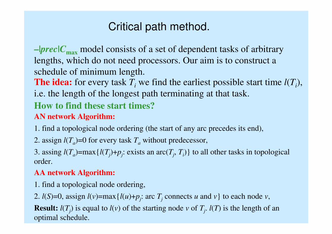
Critical path method.
–|prec|Cmax model consists of a set of dependent tasks of arbitrary
lengths, which do not need processors. Our aim is to construct a
schedule of minimum length.The idea: for every task Ti we find the earliest possible start time l(Ti),
i.e. the length of the longest path terminating at that task.
AN network Algorithm:
1. find a topological node ordering (the start of any arc precedes its end),
2. assign l(Ta)=0 for every task Ta without predecessor,
3. assing l(Ta)=max{l(Tj)+pj: exists an arc(Tj, Ti)} to all other tasks in topological
order.
AA network Algorithm:
1. find a topological node ordering,
2. l(S)=0, assign l(v)=max{l(u)+pj: arc Tj connects u and v} to each node v,
Result: l(Tj) is equal to l(v) of the starting node v of Tj. l(T) is the length of an
optimal schedule.
How to find these start times?
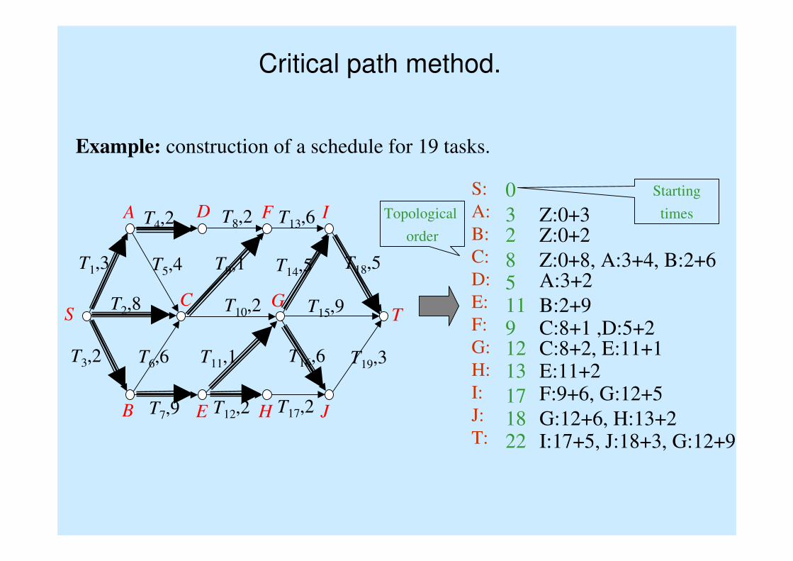
Critical path method.
Example: construction of a schedule for 19 tasks.
S:
A:
B:
C:
D:
E:
F:
G:
H:
I:
J:
T:
0
Z:0+33Z:0+22
Z:0+8, A:3+4, B:2+68A:3+25B:2+911C:8+1 ,D:5+29C:8+2, E:11+112E:11+213F:9+6, G:12+517G:12+6, H:13+218I:17+5, J:18+3, G:12+922
A
SC G
T
B E H J
D F I
T19,3
T13,6T8,2T4,2
T2,8 T10,2 T15,9
T17,2T12,2T7,9
T18,5T14,5T9,1T5,4T1,3
T3,2 T6,6 T11,1 T16,6
Topological
order
Starting
times
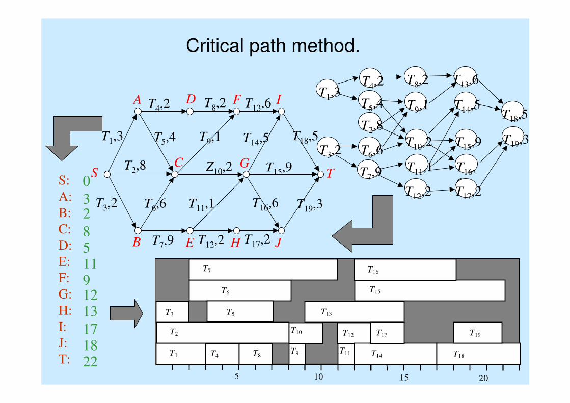
Critical path method.
5 10 15 20
T1 T4
T3
T2
T6
T5
T7
T9T8
T10
T11
T12
T13
T14
T15
T16
T17
T18
T19
S:
A:
B:
C:
D:
E:
F:
G:
H:
I:
J:
T:
0
32
851191213
171822
T1,3
T2,8
T3,2
T4,2
T5,4
T6,6
T7,9
T9,1
T10,2
T8,2
T11,1
T12,2
T14,5
T15,9
T13,6
T16,
6T17,2
T18,5
T19,3
A
SC G
T
B E H J
D F I
T19,3
T13,6T8,2T4,2
T2,8 Z10,2 T15,9
T17,2T12,2T7,9
T18,5T14,5T9,1T5,4T1,3
T3,2 T6,6 T11,1 T16,6
Critical path method.
• Critical path method does not only minimize Cmax, but also optimizes
all previously defined criteria.
• We can introduce to the model arbitrary release times by adding for
each task Tj extra task of length rj preceding Tj.
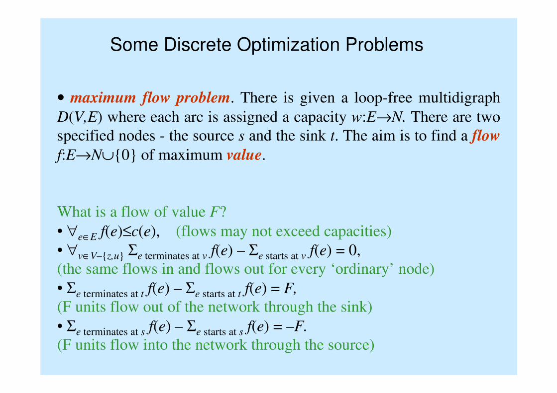
Some Discrete Optimization Problems
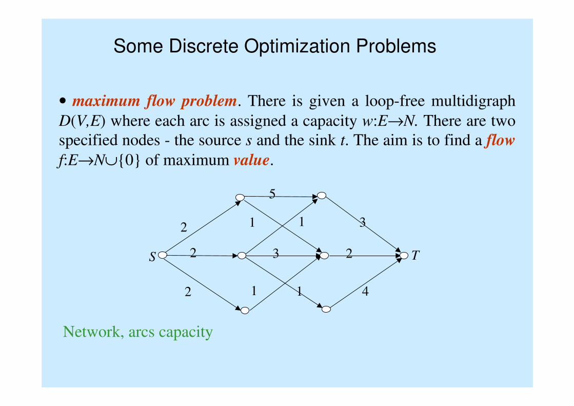
• maximum flow problem. There is given a loop-free multidigraph
D(V,E) where each arc is assigned a capacity w:E→N. There are two
specified nodes - the source s and the sink t. The aim is to find a flow
f:E→N∪{0} of maximum value.
What is a flow of value F?
• ∀e∈E f(e)≤c(e), (flows may not exceed capacities)
• ∀v∈V–{z,u} Σe terminates at v f(e) – Σe starts at v f(e) = 0,
(the same flows in and flows out for every ‘ordinary’ node)
• Σe terminates at t f(e) – Σe starts at t f(e) = F,
(F units flow out of the network through the sink)
• Σe terminates at s f(e) – Σe starts at s f(e) = –F.
(F units flow into the network through the source)
Some Discrete Optimization Problems
2
5
31 1
2 3 2
2 11 4
S T
Network, arcs capacity
• maximum flow problem. There is given a loop-free multidigraph
D(V,E) where each arc is assigned a capacity w:E→N. There are two
specified nodes - the source s and the sink t. The aim is to find a flow
f:E→N∪{0} of maximum value.

Some Discrete Optimization Problems
2/2
5/2
3/21/0 1/0
2/2 3/1 2/2
2/1 1/11/1 4/1
S T
... and maximum flow
F=5
Complexity O(|V||E|log(|V|2|E|) ≤≤≤≤O(|V|3).
• maximum flow problem. There is given a loop-free multidigraph
D(V,E) where each arc is assigned a capacity w:E→N. There are two
specified nodes - the source s and the sink t. The aim is to find a flow
f:E→N∪{0} of maximum value.
Some Discrete Optimization Problems
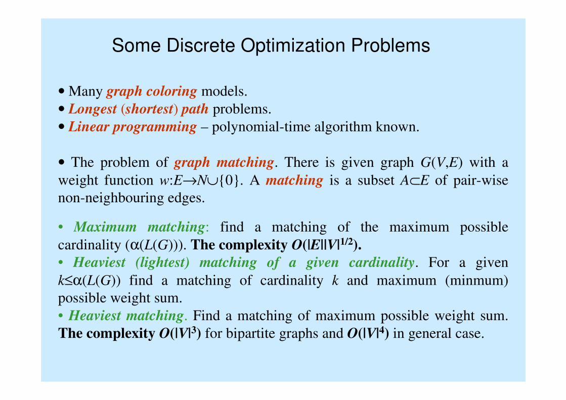
• Many graph coloring models.
• Longest (shortest) path problems.
• Linear programming – polynomial-time algorithm known.
• The problem of graph matching. There is given graph G(V,E) with a
weight function w:E→N∪{0}. A matching is a subset A⊂E of pair-wise
non-neighbouring edges.
• Maximum matching: find a matching of the maximum possible
cardinality (α(L(G))). The complexity O(|E||V|1/2).
• Heaviest (lightest) matching of a given cardinality. For a given
k≤α(L(G)) find a matching of cardinality k and maximum (minmum)
possible weight sum.
• Heaviest matching. Find a matching of maximum possible weight sum.
The complexity O(|V|3) for bipartite graphs and O(|V|4) in general case.
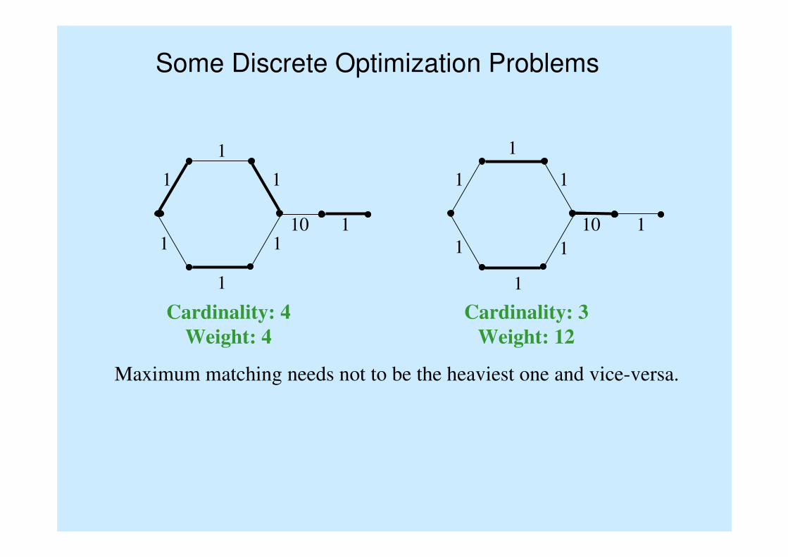
Some Discrete Optimization Problems
Cardinality: 4
Weight: 4
1
101
1 1
1
1
1
1
10 1
1 1
11
1
Cardinality: 3
Weight: 12
Maximum matching needs not to be the heaviest one and vice-versa.
M 1
M 2
M 3
5
M 1
M 2
M 3
Z 1
5
M 1
M 2
M 3
Z 1
5
Z 2
Z 2 M 1
M 2
M 3
Z 1
5
Z 2
Z 2
Z 3
Z 3
M 1
M 2
M 3
Z 1
5
Z 2
Z 2
Z 4 Z 3
Z 3
M1
M2
M3
T 1
5
T 2
T 2
T 5T 4T 3
T 3
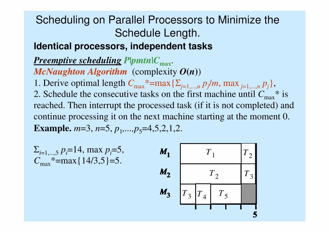
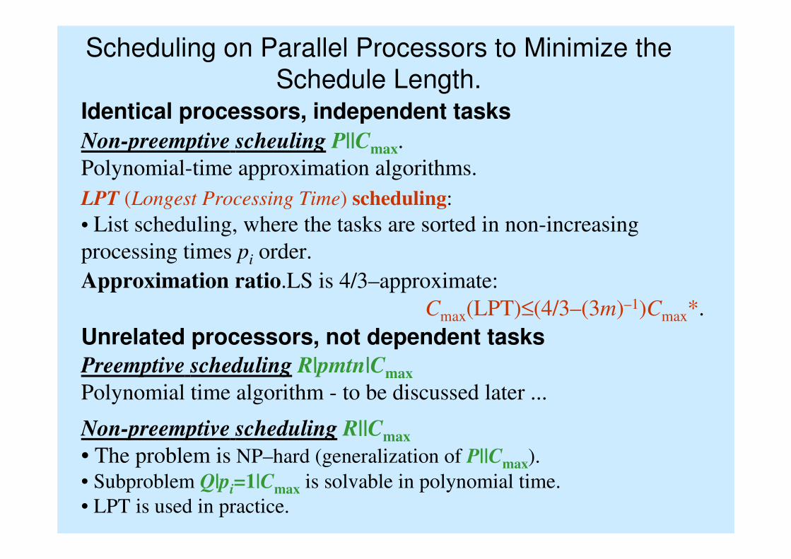
Scheduling on Parallel Processors to Minimize the
Schedule Length.Identical processors, independent tasks
Preemptive scheduling P|pmtn|Cmax.
McNaughton Algorithm (complexity O(n))
1. Derive optimal length Cmax*=max{Σj=1,...,n pj/m, max j=1,...,n pj},
2. Schedule the consecutive tasks on the first machine until Cmax* is
reached. Then interrupt the processed task (if it is not completed) and
continue processing it on the next machine starting at the moment 0.
Example. m=3, n=5, p1,...,p5=4,5,2,1,2.
Σi=1,...,5 pi=14, max pi=5,
Cmax*=max{14/3,5}=5.
Scheduling on Parallel Processors to Minimize the
Schedule Length.Identical processors, independent tasks
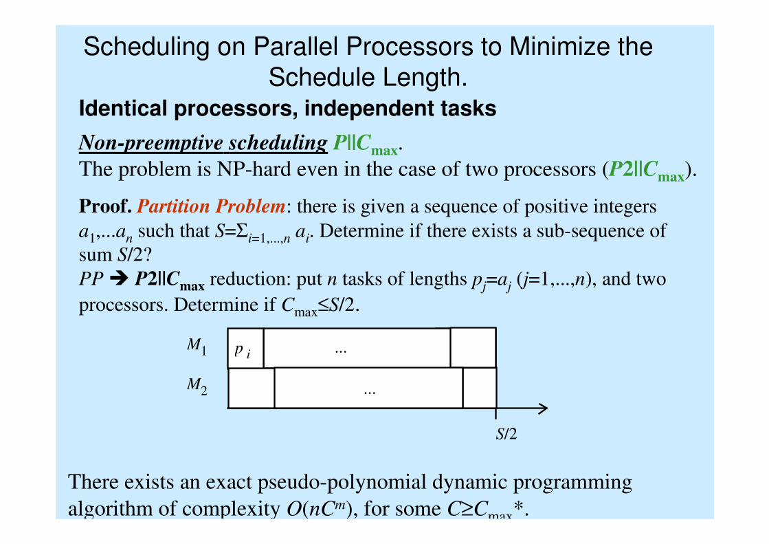
Non-preemptive scheduling P||Cmax.
The problem is NP-hard even in the case of two processors (P2||Cmax).
Proof. Partition Problem: there is given a sequence of positive integers
a1,...an such that S=Σi=1,...,n ai. Determine if there exists a sub-sequence of
sum S/2?
PP � P2||Cmax reduction: put n tasks of lengths pj=aj (j=1,...,n), and two
processors. Determine if Cmax≤S/2.
M1
M2
S/2
p i ...
...
There exists an exact pseudo-polynomial dynamic programming
algorithm of complexity O(nCm), for some C≥Cmax*.
Scheduling on Parallel Processors to Minimize the
Schedule Length.Identical processors, independent tasks
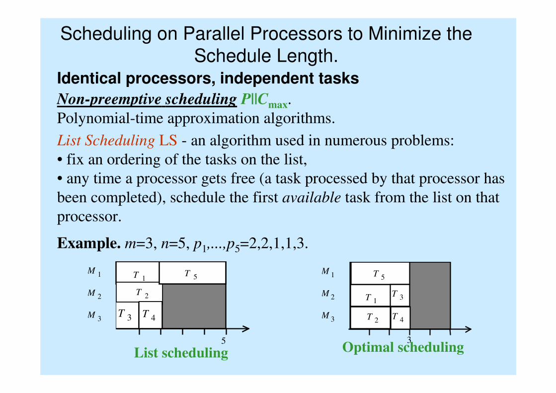
Non-preemptive scheduling P||Cmax.
Polynomial-time approximation algorithms.
List Scheduling LS - an algorithm used in numerous problems:
• fix an ordering of the tasks on the list,
• any time a processor gets free (a task processed by that processor has
been completed), schedule the first available task from the list on that
processor.
Example. m=3, n=5, p1,...,p5=2,2,1,1,3.
M 1
M 2
M 3
5
List scheduling Optimal scheduling
M 1
M 2
M 3 T 2
3
T 1
T 5
T 3
T 4
T 1
T 2
T 3 T 4
T 5
Scheduling on Parallel Processors to Minimize the
Schedule Length.Identical processors, independent tasks
Non-preemptive scheduling P||Cmax.
Polynomial-time approximation algorithms.
List Scheduling LS - an algorithm used in numerous problems:
• fix an ordering of the tasks on the list,
• any time a processor gets free (a task processed by that processor has
been completed), schedule the first available task from the list on that
processor.
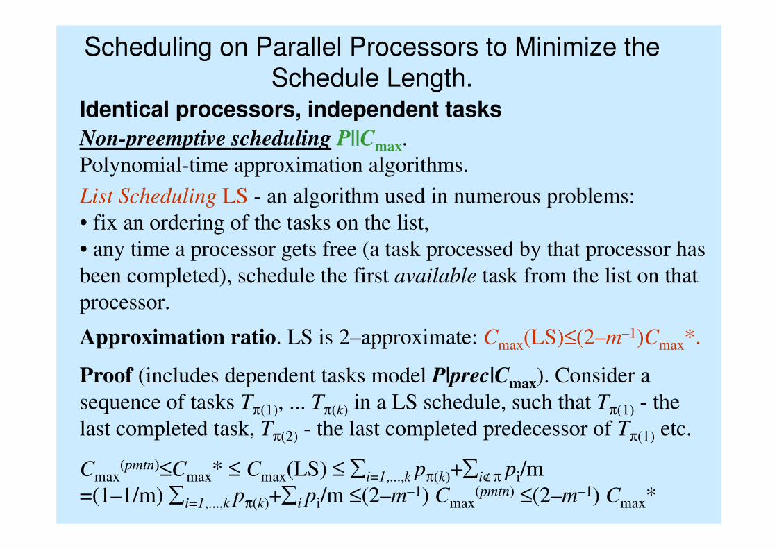
Approximation ratio. LS is 2–approximate: Cmax(LS)≤(2–m–1)Cmax*.
Proof (includes dependent tasks model P|prec|Cmax). Consider a
sequence of tasks Tπ(1), ... Tπ(k) in a LS schedule, such that Tπ(1) - the
last completed task, Tπ(2) - the last completed predecessor of Tπ(1) etc.
Cmax(pmtn)≤Cmax* ≤ Cmax(LS) ≤ ∑i=1,...,k pπ(k)+∑i∉π pi/m
=(1–1/m) ∑i=1,...,k pπ(k)+∑i pi/m ≤(2–m–1) Cmax(pmtn) ≤(2–m–1) Cmax*
Scheduling on Parallel Processors to Minimize the
Schedule Length.Identical processors, independent tasks
Non-preemptive scheduling P||Cmax.
Polynomial-time approximation algorithms.
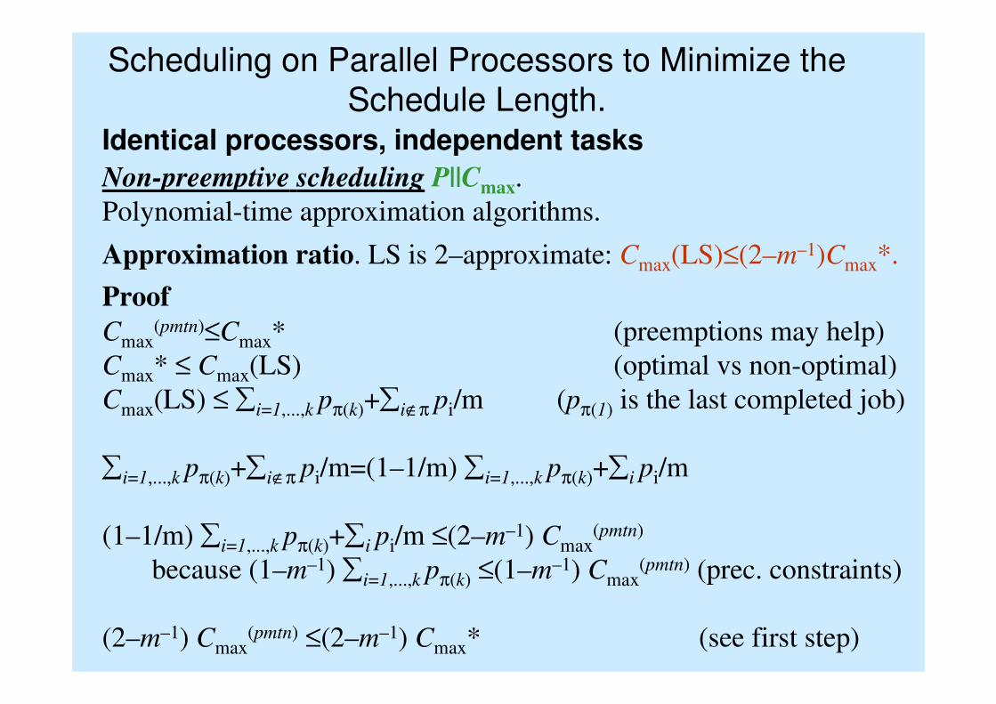
Approximation ratio. LS is 2–approximate: Cmax(LS)≤(2–m–1)Cmax*.
Proof
Cmax(pmtn)≤Cmax* (preemptions may help)
Cmax* ≤ Cmax(LS) (optimal vs non-optimal)
Cmax(LS) ≤ ∑i=1,...,k pπ(k)+∑i∉π pi/m (pπ(1) is the last completed job)
∑i=1,...,k pπ(k)+∑i∉π pi/m=(1–1/m) ∑i=1,...,k pπ(k)+∑i pi/m
(1–1/m) ∑i=1,...,k pπ(k)+∑i pi/m ≤(2–m–1) Cmax(pmtn)
because (1–m–1) ∑i=1,...,k pπ(k) ≤(1–m–1) Cmax(pmtn) (prec. constraints)
(2–m–1) Cmax(pmtn) ≤(2–m–1) Cmax* (see first step)
Scheduling on Parallel Processors to Minimize the
Schedule Length.Identical processors, independent tasks
Non-preemptive scheuling P||Cmax.
Polynomial-time approximation algorithms.
LPT (Longest Processing Time) scheduling:
• List scheduling, where the tasks are sorted in non-increasing
processing times pi order.
Approximation ratio.LS is 4/3–approximate:
Cmax(LPT)≤(4/3–(3m)–1)Cmax*.
Unrelated processors, not dependent tasks
Preemptive scheduling R|pmtn|Cmax
Polynomial time algorithm - to be discussed later ...
Non-preemptive scheduling R||Cmax
• The problem is NP–hard (generalization of P||Cmax).
• Subproblem Q|pi=1|Cmax is solvable in polynomial time.
• LPT is used in practice.
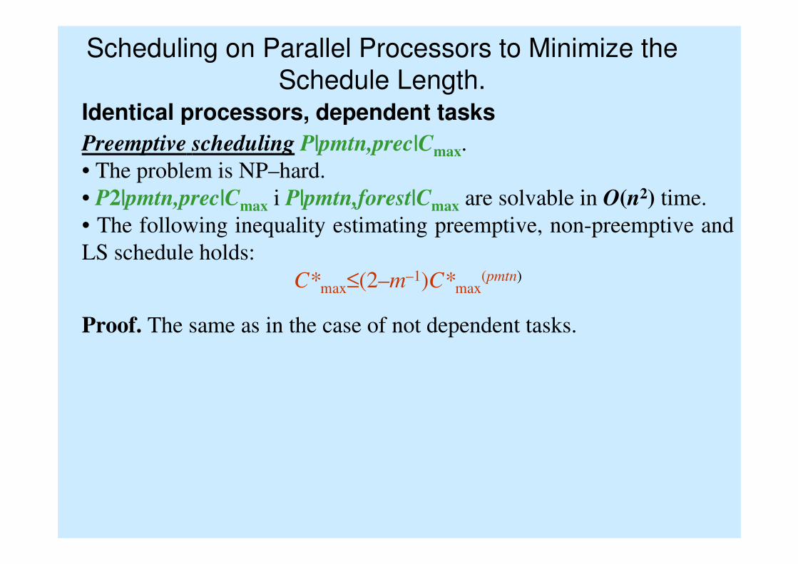
Scheduling on Parallel Processors to Minimize the
Schedule Length.Identical processors, dependent tasks
Preemptive scheduling P|pmtn,prec|Cmax.
• The problem is NP–hard.
• P2|pmtn,prec|Cmax i P|pmtn,forest|Cmax are solvable in O(n2) time.
• The following inequality estimating preemptive, non-preemptive and
LS schedule holds:
C*max≤(2–m–1)C*max(pmtn)
Proof. The same as in the case of not dependent tasks.
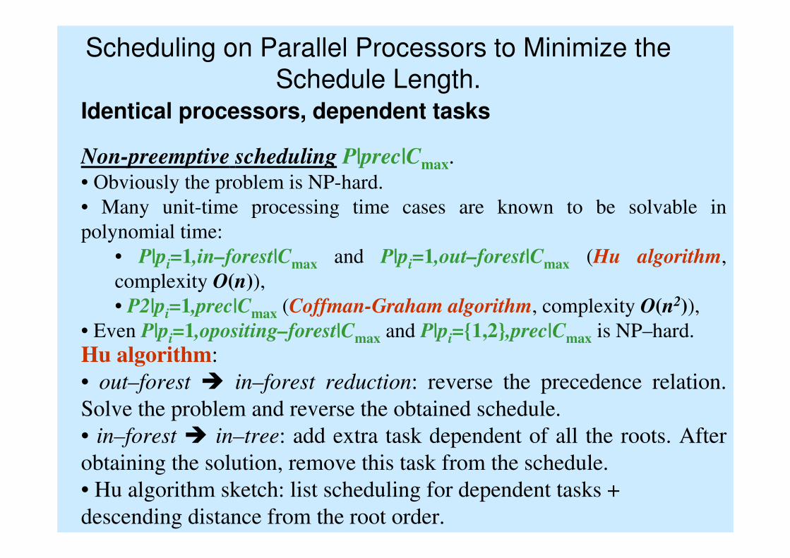
Scheduling on Parallel Processors to Minimize the
Schedule Length.Identical processors, dependent tasks
Non-preemptive scheduling P|prec|Cmax.• Obviously the problem is NP-hard.
• Many unit-time processing time cases are known to be solvable in
polynomial time:
• P|pi=1,in–forest|Cmax and P|pi=1,out–forest|Cmax (Hu algorithm,
complexity O(n)),
• P2|pi=1,prec|Cmax (Coffman-Graham algorithm, complexity O(n2)),
• Even P|pi=1,opositing–forest|Cmax and P|pi={1,2},prec|Cmax is NP–hard.
Hu algorithm:
• out–forest � in–forest reduction: reverse the precedence relation.
Solve the problem and reverse the obtained schedule.
• in–forest � in–tree: add extra task dependent of all the roots. After
obtaining the solution, remove this task from the schedule.
• Hu algorithm sketch: list scheduling for dependent tasks +
descending distance from the root order.
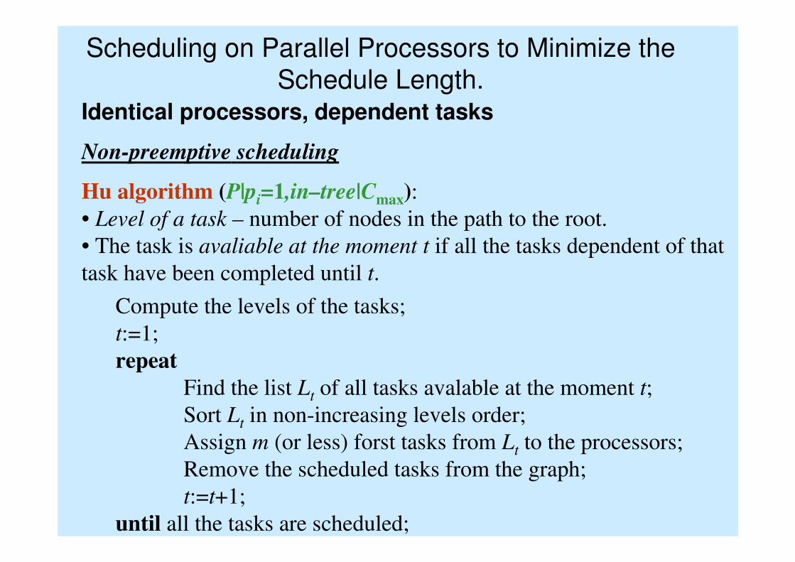
Scheduling on Parallel Processors to Minimize the
Schedule Length.Identical processors, dependent tasks
Non-preemptive scheduling
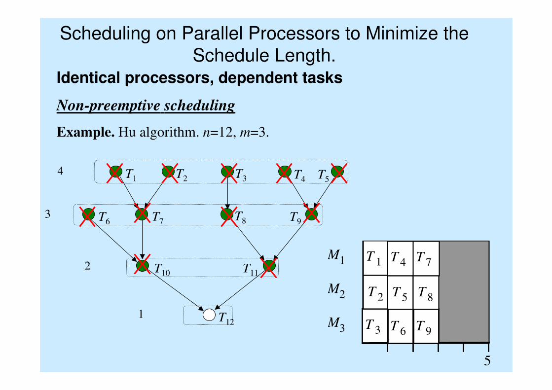
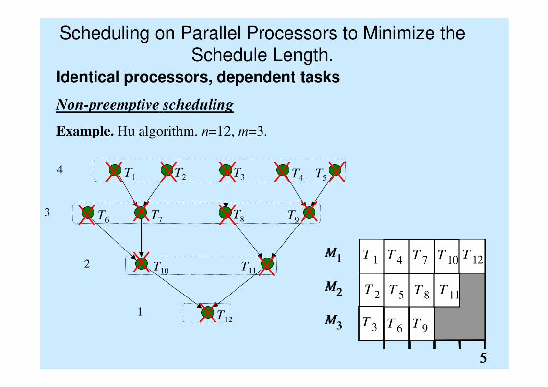
Hu algorithm (P|pi=1,in–tree|Cmax):
• Level of a task – number of nodes in the path to the root.
• The task is avaliable at the moment t if all the tasks dependent of that
task have been completed until t.
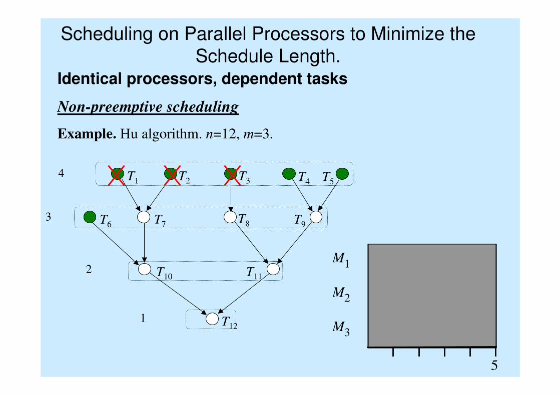
Compute the levels of the tasks;
t:=1;
repeat
Find the list Lt of all tasks avalable at the moment t;
Sort Lt in non-increasing levels order;
Assign m (or less) forst tasks from Lt to the processors;
Remove the scheduled tasks from the graph;
t:=t+1;
until all the tasks are scheduled;
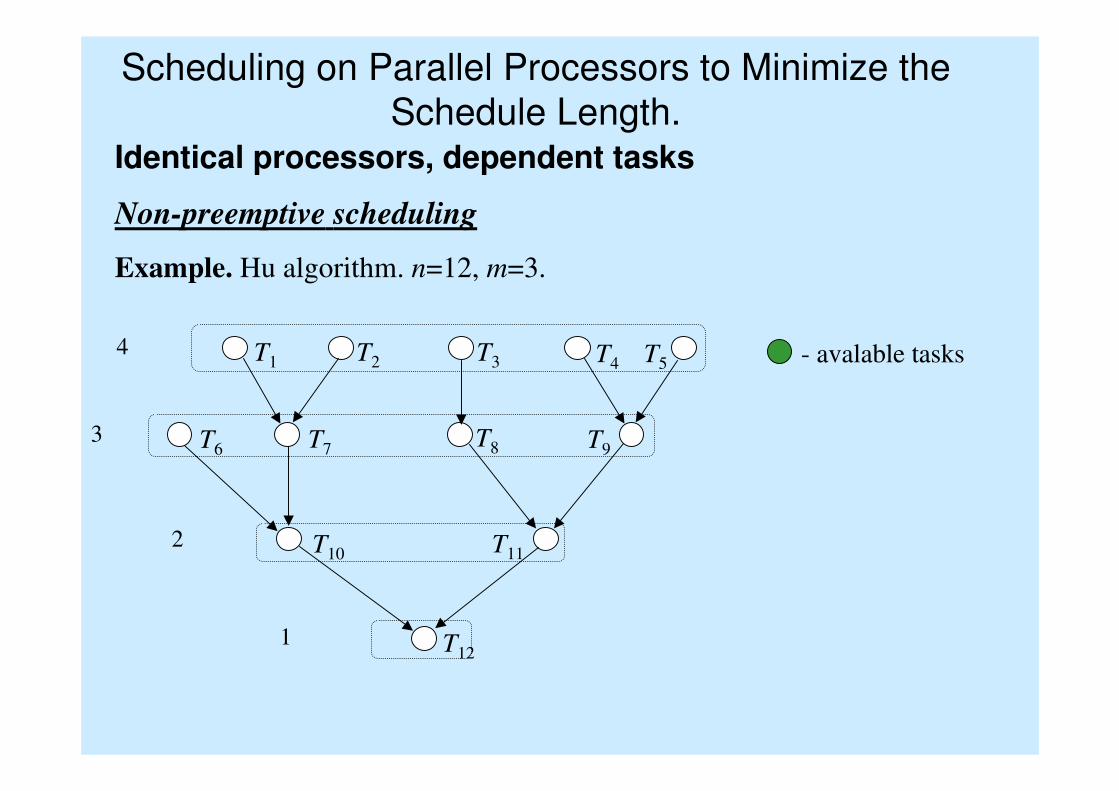
Scheduling on Parallel Processors to Minimize the
Schedule Length.Identical processors, dependent tasks
Non-preemptive scheduling
Example. Hu algorithm. n=12, m=3.
T1 T2 T3 T4 T5
T7T6
T10
T9T8
T11
T121
2
3
4 - avalable tasks
Scheduling on Parallel Processors to Minimize the
Schedule Length.Identical processors, dependent tasks
Non-preemptive scheduling
Example. Hu algorithm. n=12, m=3.
T1 T2 T3 T4 T5
T7T6
T10
T9T8
T11
T121
2
3
4
M 1
M 2
M 3
5
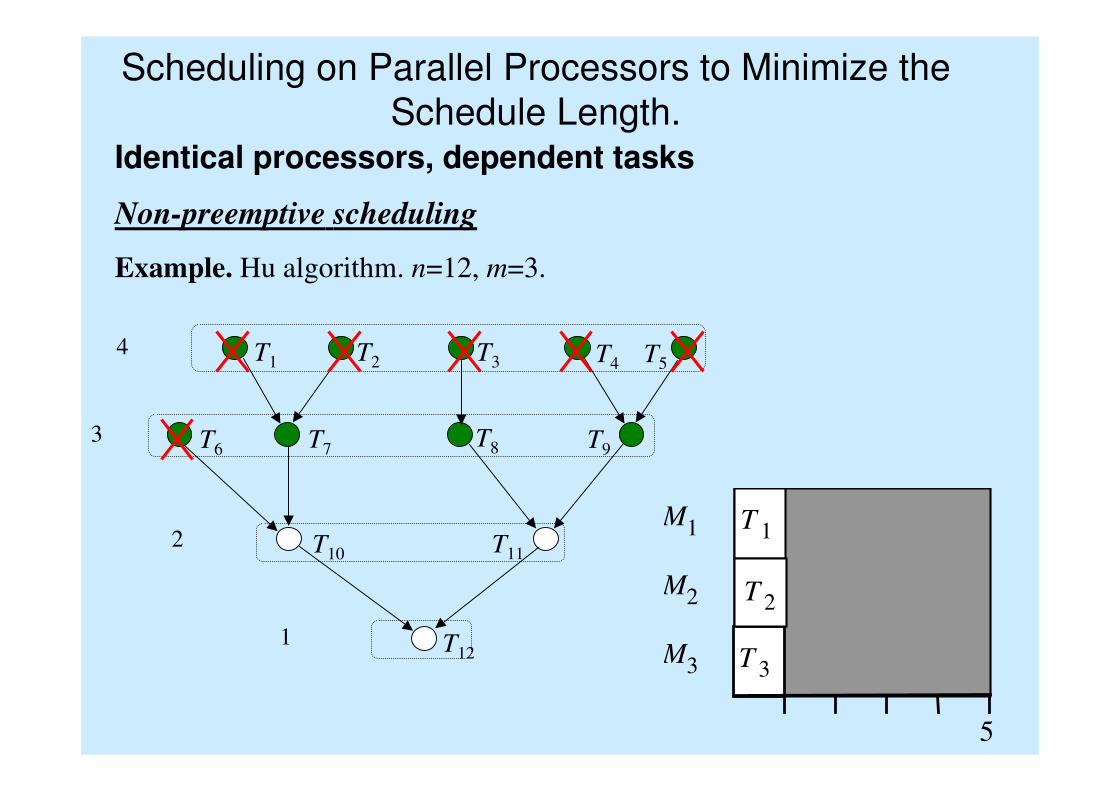
Scheduling on Parallel Processors to Minimize the
Schedule Length.Identical processors, dependent tasks
Non-preemptive scheduling
Example. Hu algorithm. n=12, m=3.
T1 T2 T3 T4 T5
T7T6
T10
T9T8
T11
T121
2
3
4
M1
M2
M3
5
T 1
T 3
T 2
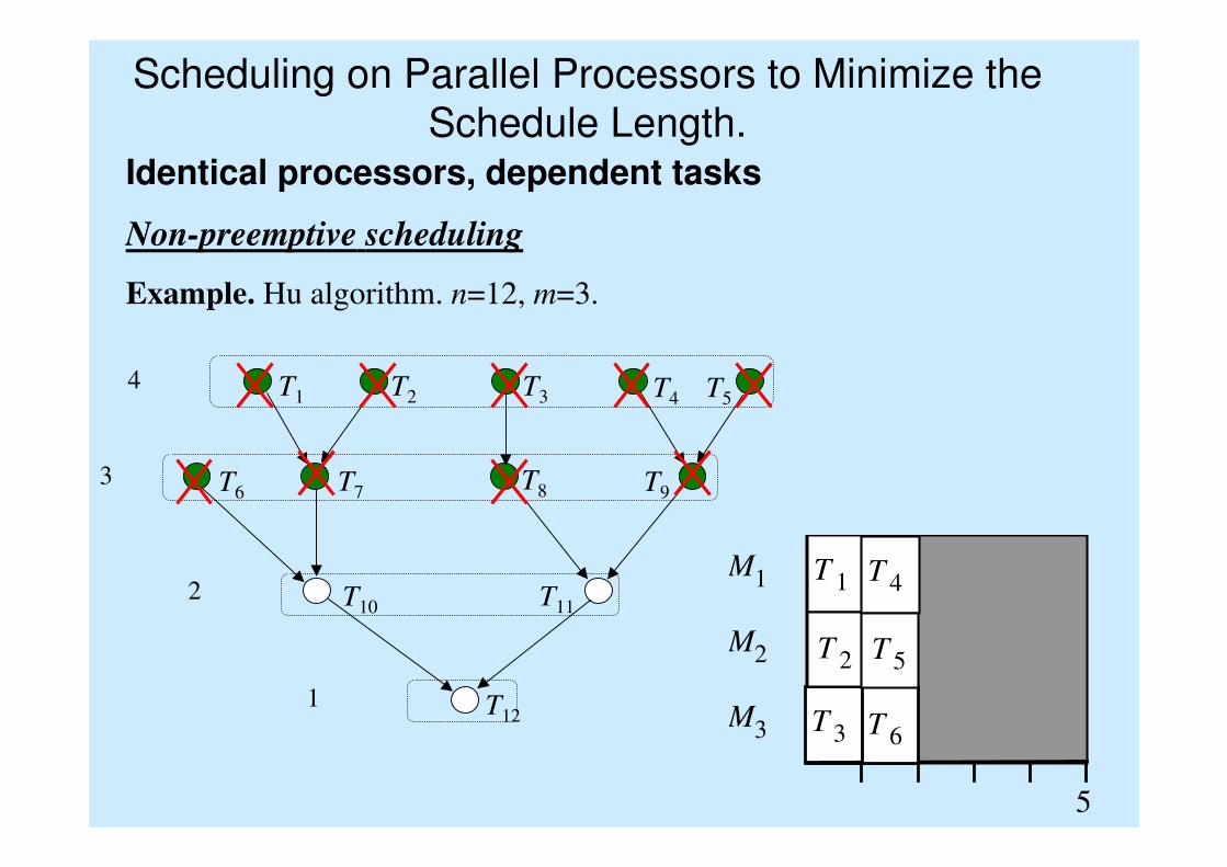
Scheduling on Parallel Processors to Minimize the
Schedule Length.Identical processors, dependent tasks
Non-preemptive scheduling
Example. Hu algorithm. n=12, m=3.
T1 T2 T3 T4 T5
T7T6
T10
T9T8
T11
T121
2
3
4
M1
M2
M3
5
T 1
T 6T 3
T 2
T 4
T 5
Scheduling on Parallel Processors to Minimize the
Schedule Length.Identical processors, dependent tasks
Non-preemptive scheduling
Example. Hu algorithm. n=12, m=3.
T1 T2 T3 T4 T5
T7T6
T10
T9T8
T11
T121
2
3
4
M1
M2
M3
5
T 1
T 6T 3
T 2
T 4
T 5
T 9
T 7
T 8
Scheduling on Parallel Processors to Minimize the
Schedule Length.Identical processors, dependent tasks
Non-preemptive scheduling
Example. Hu algorithm. n=12, m=3.
T1 T2 T3 T4 T5
T7T6
T10
T9T8
T11
T121
2
3
4
M 1
M 2
M 3
5
Z 1
Z 6 Z 3
Z 2
Z 4
Z 5
Z 9
Z 7
Z 8
Z 10
Z 11
M1
M2
M3
5
T 1
T 6T 3
T 2
T 4
T 5
T 9
T 7
T 8
T 10
T 11
T 12

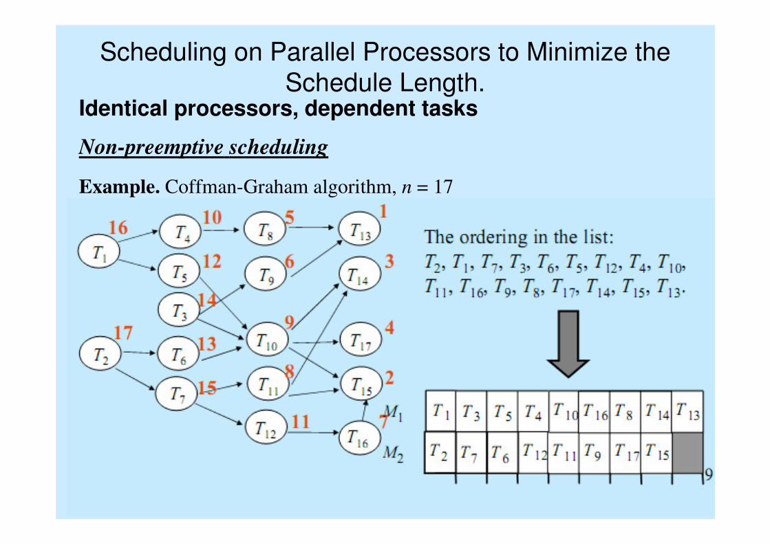
Non-preemptive scheduling
Coffman-Graham algorithm (P2|prec|Cmax):
1. label the tasks with integers l from range [1, ..., n]
2. list scheduling, with desscening labels order.
Phase 1 - task labeling;
no task has any label or list at the beginning;
for i:=1 to n do begin
A:=the set of tasks without label, for which all dependent
tasks are labeled;
for each T∈A do assign the descending sequence of the labels of
tasks dependent of T to list(T);
choose T ∈ A with the lexicographic minimum list(T);
l(T):=i;
end;
Identical processors, dependent tasks
Scheduling on Parallel Processors to Minimize the
Schedule Length.
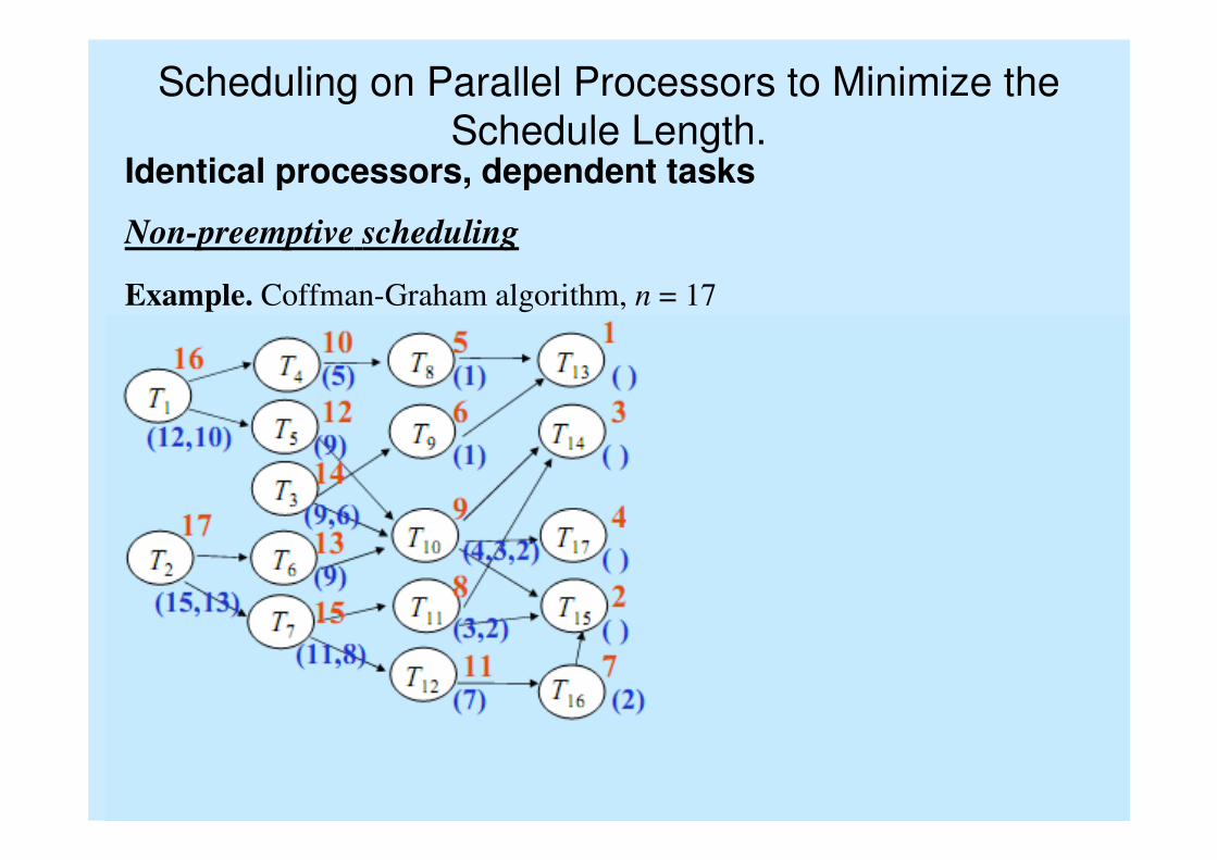
Non-preemptive scheduling
Example. Coffman-Graham algorithm, n = 17
Identical processors, dependent tasks
Scheduling on Parallel Processors to Minimize the
Schedule Length.
Non-preemptive scheduling
Example. Coffman-Graham algorithm, n = 17
Identical processors, dependent tasks
Scheduling on Parallel Processors to Minimize the
Schedule Length.
Scheduling on Parallel Processors to Minimize the
Schedule Length.Identical processors, dependent tasks
Non-preemptive scheduling
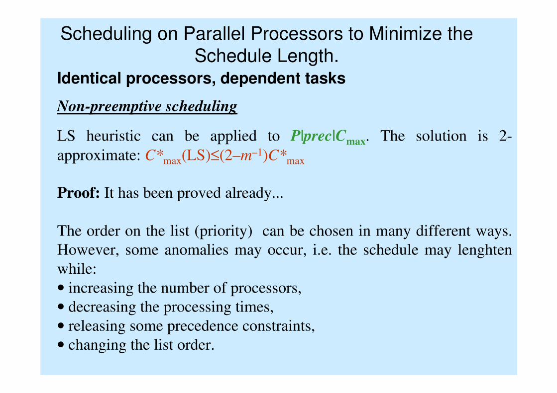
LS heuristic can be applied to P|prec|Cmax. The solution is 2-
approximate: C*max(LS)≤(2–m–1)C*max
Proof: It has been proved already...
The order on the list (priority) can be chosen in many different ways.
However, some anomalies may occur, i.e. the schedule may lenghten
while:
• increasing the number of processors,
• decreasing the processing times,
• releasing some precedence constraints,
• changing the list order.
Scheduling on Parallel Processors
to Minimize the Mean Flow TimeIdentical processors, independent tasks
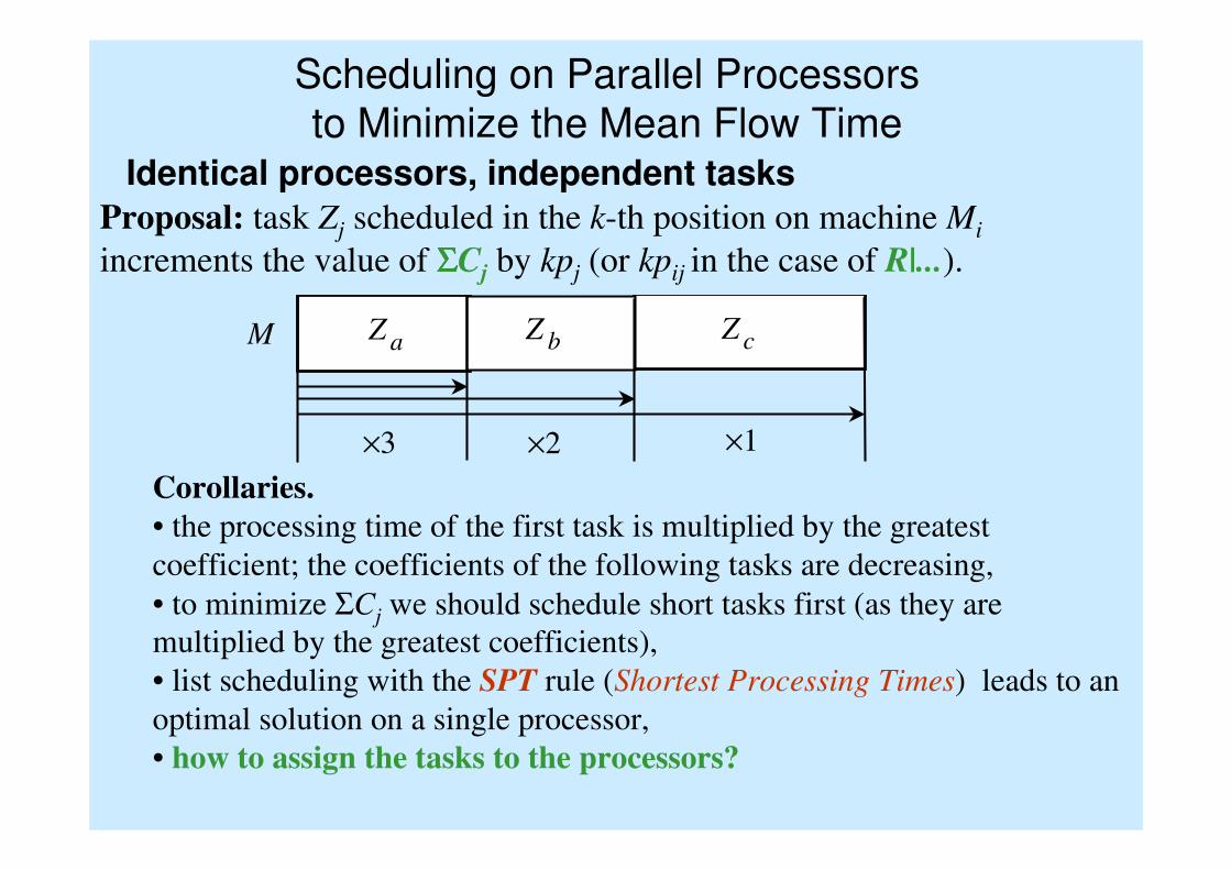
Corollaries.
• the processing time of the first task is multiplied by the greatest
coefficient; the coefficients of the following tasks are decreasing,
• to minimize ΣCj we should schedule short tasks first (as they are
multiplied by the greatest coefficients),
• list scheduling with the SPT rule (Shortest Processing Times) leads to an
optimal solution on a single processor,
• how to assign the tasks to the processors?
Proposal: task Zj scheduled in the k-th position on machine Mi
increments the value of ΣΣΣΣCj by kpj (or kpij in the case of R|...).
M Z a Z c Z b
×3 ×2 ×1
Scheduling on Parallel Processors
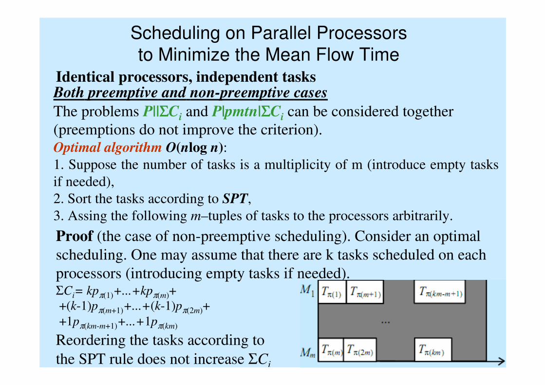
to Minimize the Mean Flow TimeIdentical processors, independent tasksBoth preemptive and non-preemptive cases
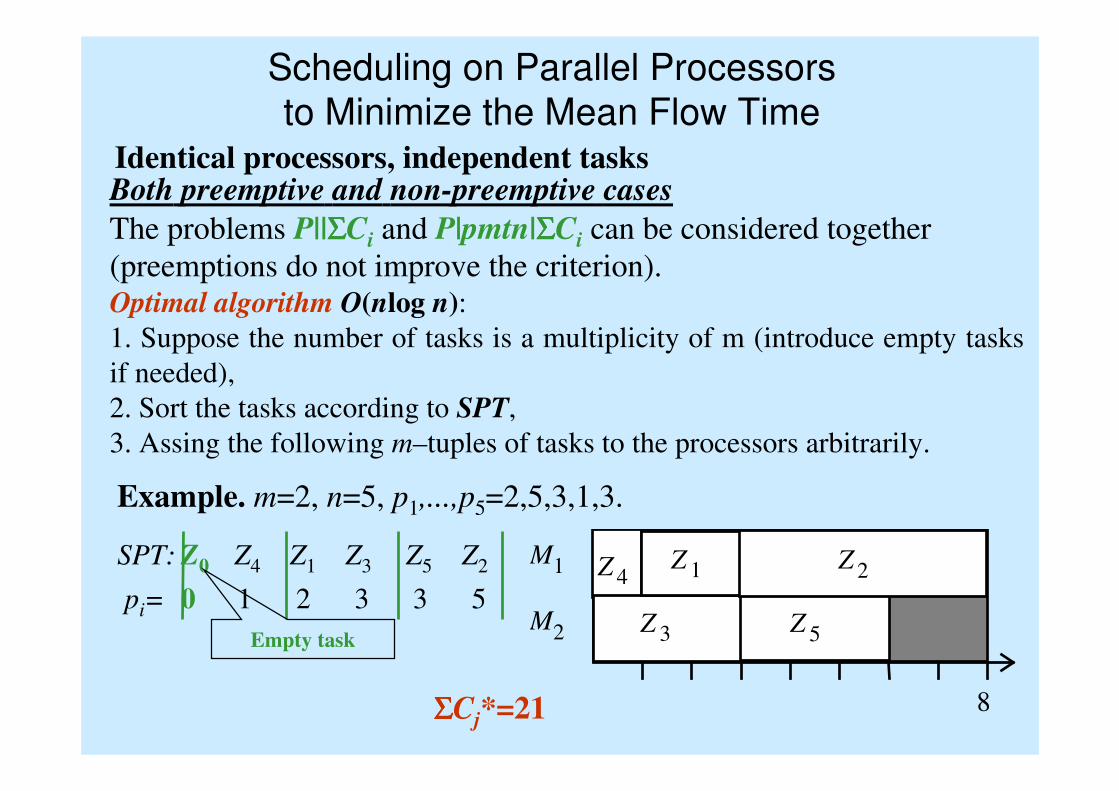
The problems P||ΣΣΣΣCi and P|pmtn|ΣΣΣΣCi can be considered together
(preemptions do not improve the criterion).Optimal algorithm O(nlog n):
1. Suppose the number of tasks is a multiplicity of m (introduce empty tasks
if needed),
2. Sort the tasks according to SPT,
3. Assing the following m–tuples of tasks to the processors arbitrarily.
Example. m=2, n=5, p1,...,p5=2,5,3,1,3.
SPT: Z4 Z1 Z3 Z5 Z2
pi= 1 2 3 3 5
M 1
M 2
8
Z 4
Z 3
Z 1
Z 5
Z 2
ΣΣΣΣCj*=21
Z0
0
Empty task
Scheduling on Parallel Processors
to Minimize the Mean Flow TimeIdentical processors, independent tasksBoth preemptive and non-preemptive cases
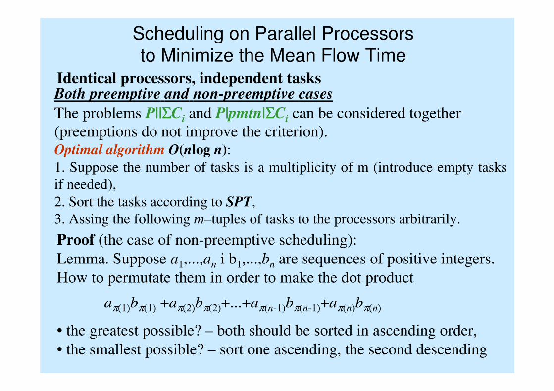
The problems P||ΣΣΣΣCi and P|pmtn|ΣΣΣΣCi can be considered together
(preemptions do not improve the criterion).Optimal algorithm O(nlog n):
1. Suppose the number of tasks is a multiplicity of m (introduce empty tasks
if needed),
2. Sort the tasks according to SPT,
3. Assing the following m–tuples of tasks to the processors arbitrarily.
Proof (the case of non-preemptive scheduling):
Lemma. Suppose a1,...,an i b1,...,bn are sequences of positive integers.
How to permutate them in order to make the dot product
aπ(1)bπ(1) +aπ(2)bπ(2)+...+aπ(n-1)bπ(n-1)+aπ(n)bπ(n)
• the greatest possible? – both should be sorted in ascending order,
• the smallest possible? – sort one ascending, the second descending
Scheduling on Parallel Processors
to Minimize the Mean Flow TimeIdentical processors, independent tasksBoth preemptive and non-preemptive cases
The problems P||ΣΣΣΣCi and P|pmtn|ΣΣΣΣCi can be considered together
(preemptions do not improve the criterion).Optimal algorithm O(nlog n):
1. Suppose the number of tasks is a multiplicity of m (introduce empty tasks
if needed),
2. Sort the tasks according to SPT,
3. Assing the following m–tuples of tasks to the processors arbitrarily.
Proof (the case of non-preemptive scheduling). Consider an optimal
scheduling. One may assume that there are k tasks scheduled on each
processors (introducing empty tasks if needed).ΣCi= kpπ(1)+...+kpπ(m)+
+(k-1)pπ(m+1)+...+(k-1)pπ(2m)+
+1pπ(km-m+1)+...+1pπ(km)
Reordering the tasks according to
the SPT rule does not increase ΣCi
Scheduling on Parallel Processors
to Minimize the Mean Flow TimeIdentical processors, independent tasks
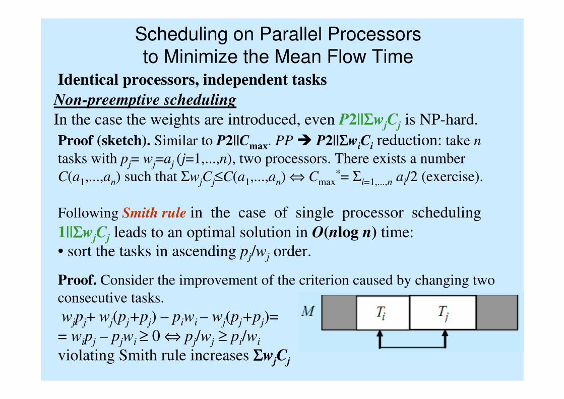
Non-preemptive scheduling
In the case the weights are introduced, even P2||ΣΣΣΣwjCj is NP-hard.
Proof (sketch). Similar to P2||Cmax. PP � P2||ΣΣΣΣwiCi reduction: take n
tasks with pj= wj=aj (j=1,...,n), two processors. There exists a number
C(a1,...,an) such that ΣwjCj≤C(a1,...,an) ⇔ Cmax*= Σi=1,...,n ai/2 (exercise).
Following Smith rule in the case of single processor scheduling
1||ΣΣΣΣwjCj leads to an optimal solution in O(nlog n) time:
• sort the tasks in ascending pj/wj order.
Proof. Consider the improvement of the criterion caused by changing two
consecutive tasks.
wjpj+ wj(pj+pj) – piwi – wj(pj+pj)=
= wipj – pjwi ≥ 0 ⇔ pj/wj ≥ pi/wi
violating Smith rule increases ΣΣΣΣwjCj
Scheduling on Parallel Processorsto Minimize the Mean Flow Time
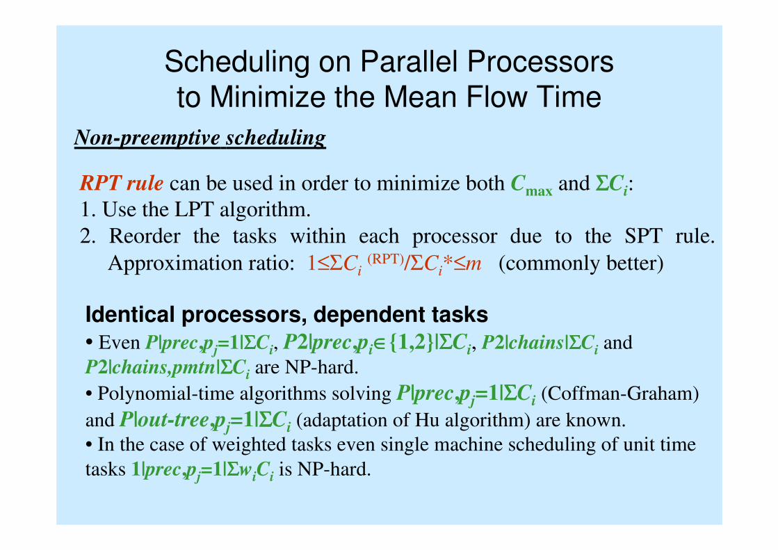
RPT rule can be used in order to minimize both Cmax and ΣΣΣΣCi:
1. Use the LPT algorithm.
2. Reorder the tasks within each processor due to the SPT rule.
Approximation ratio: 1≤ΣCi (RPT)/ΣCi*≤m (commonly better)
Identical processors, dependent tasks
• Even P|prec,pj=1|ΣΣΣΣCi, P2|prec,pi∈∈∈∈{1,2}|ΣΣΣΣCi, P2|chains|ΣΣΣΣCi and
P2|chains,pmtn|ΣΣΣΣCi are NP-hard.
• Polynomial-time algorithms solving P|prec,pj=1|ΣΣΣΣCi (Coffman-Graham)
and P|out-tree,pj=1|ΣΣΣΣCi (adaptation of Hu algorithm) are known.
• In the case of weighted tasks even single machine scheduling of unit time
tasks 1|prec,pj=1|ΣΣΣΣwiCi is NP-hard.
Non-preemptive scheduling
Scheduling on Parallel Processors
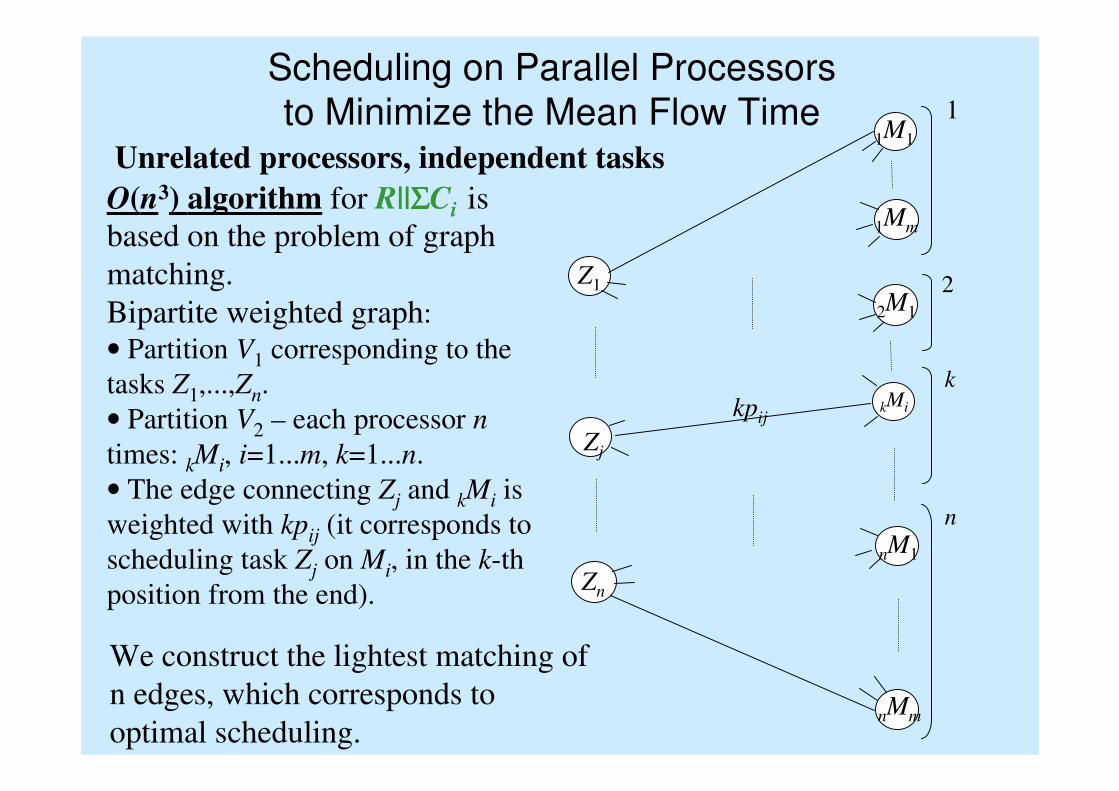
to Minimize the Mean Flow TimeUnrelated processors, independent tasks
O(n3) algorithm for R||ΣΣΣΣCi is
based on the problem of graph
matching.
Bipartite weighted graph:
• Partition V1 corresponding to the
tasks Z1,...,Zn.
• Partition V2 – each processor n
times: kMi, i=1...m, k=1...n.
• The edge connecting Zj and kMi is
weighted with kpij (it corresponds to
scheduling task Zj on Mi, in the k-th
position from the end).
kpij
Z1
Zj
Zn
1M1
1Mm
2M1
nMm
nM1
kMi
2
k
n
1
We construct the lightest matching of
n edges, which corresponds to
optimal scheduling.
Scheduling on Parallel Processors
to Minimize the Maximum Lateness
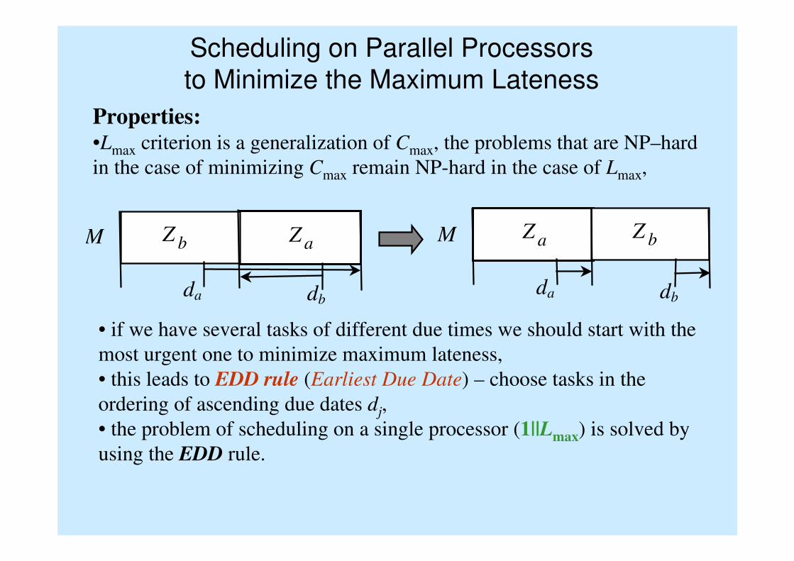
Properties:•Lmax criterion is a generalization of Cmax, the problems that are NP–hard
in the case of minimizing Cmax remain NP-hard in the case of Lmax,
• if we have several tasks of different due times we should start with the
most urgent one to minimize maximum lateness,
• this leads to EDD rule (Earliest Due Date) – choose tasks in the
ordering of ascending due dates dj,
• the problem of scheduling on a single processor (1||Lmax) is solved by
using the EDD rule.
M Z a Z b
da db
M Z a Z b
da db
Scheduling on Parallel Processors
to Minimize the Maximum Lateness
Identical processors, independent tasksPreemptive scheduling
Single machine: Liu algorithm O(n2), based on the EDD rule, solves
1|ri,pmtn|Lmax:
1. Choose the task of the smallest due date among available ones,
2. Every time a task has been completed or a new task has arrived go
to 1. (in the latter case we preempt currently processed task).
Arbitrary number of processors(P|ri,pmtn|Lmax). A polynomial-time
algorithm is known:
We use sub-routine solving the problem with deadlines
P|ri,Ci≤≤≤≤di,pmtn|–, We find the optimal value of Lmax using binary
search algorithm.
Scheduling on Parallel Processors
to Minimize the Maximum Lateness
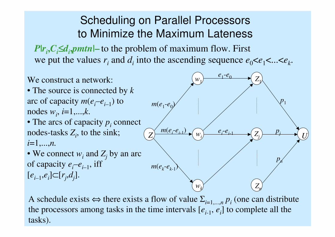
P|ri,Ci≤≤≤≤di,pmtn|– to the problem of maximum flow. First
we put the values ri and di into the ascending sequence e0<e1<...<ek.
m(e1-e0)
m(ei-ei-1)Z U
w1
wi
wk
Z1
Zj
Zn
m(ek-ek-1)
p1
pj
pn
e1-e0
ei-ei-1
We construct a network:
• The source is connected by k
arc of capacity m(ei–ei–1) to
nodes wi, i=1,...,k.
• The arcs of capacity pi connect
nodes-tasks Zi, to the sink;
i=1,...,n.
• We connect wi and Zj by an arc
of capacity ei–ei–1, iff
[ei–1,ei]⊂[rj,dj].
A schedule exists ⇔ there exists a flow of value Σi=1,...,n pi (one can distribute
the processors among tasks in the time intervals [ei-1, ei] to complete all the
tasks).
Scheduling on Parallel Processors
to Minimize the Maximum Lateness
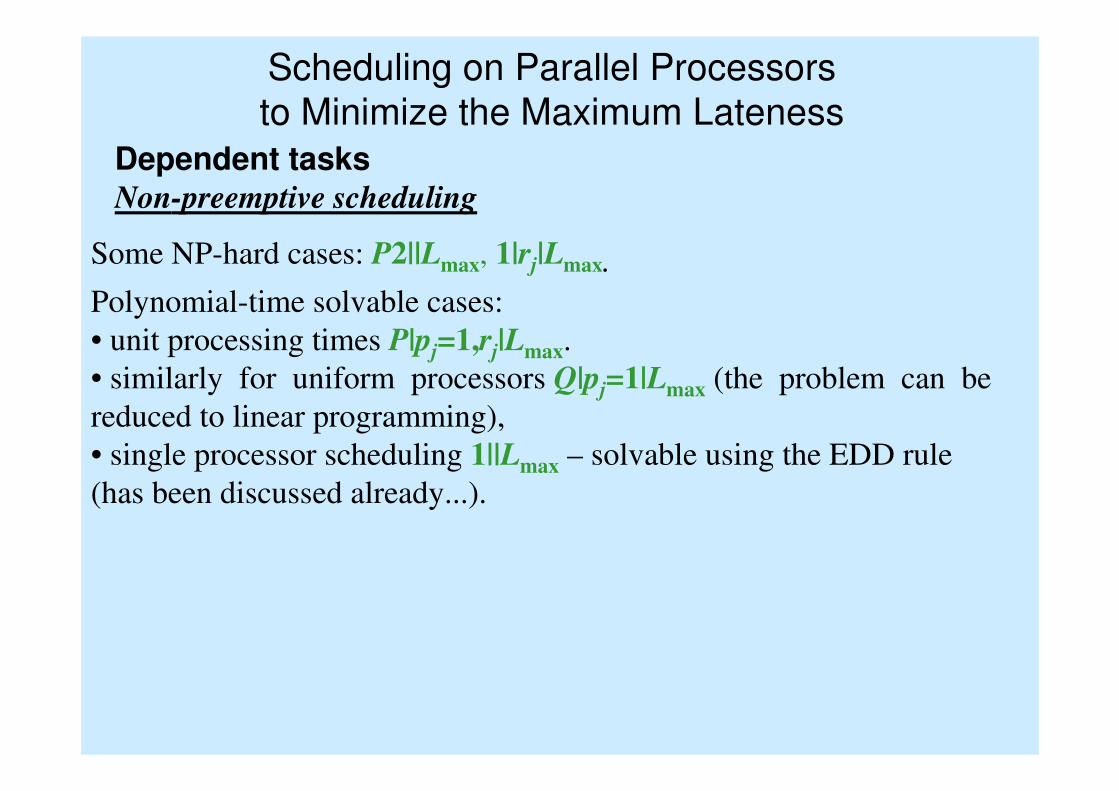
Some NP-hard cases: P2||Lmax, 1|rj|Lmax.
Dependent tasksNon-preemptive scheduling
Polynomial-time solvable cases:
• unit processing times P|pj=1,rj|Lmax.
• similarly for uniform processors Q|pj=1|Lmax (the problem can be
reduced to linear programming),
• single processor scheduling 1||Lmax – solvable using the EDD rule
(has been discussed already...).
Scheduling on Parallel Processors
to Minimize the Maximum Lateness
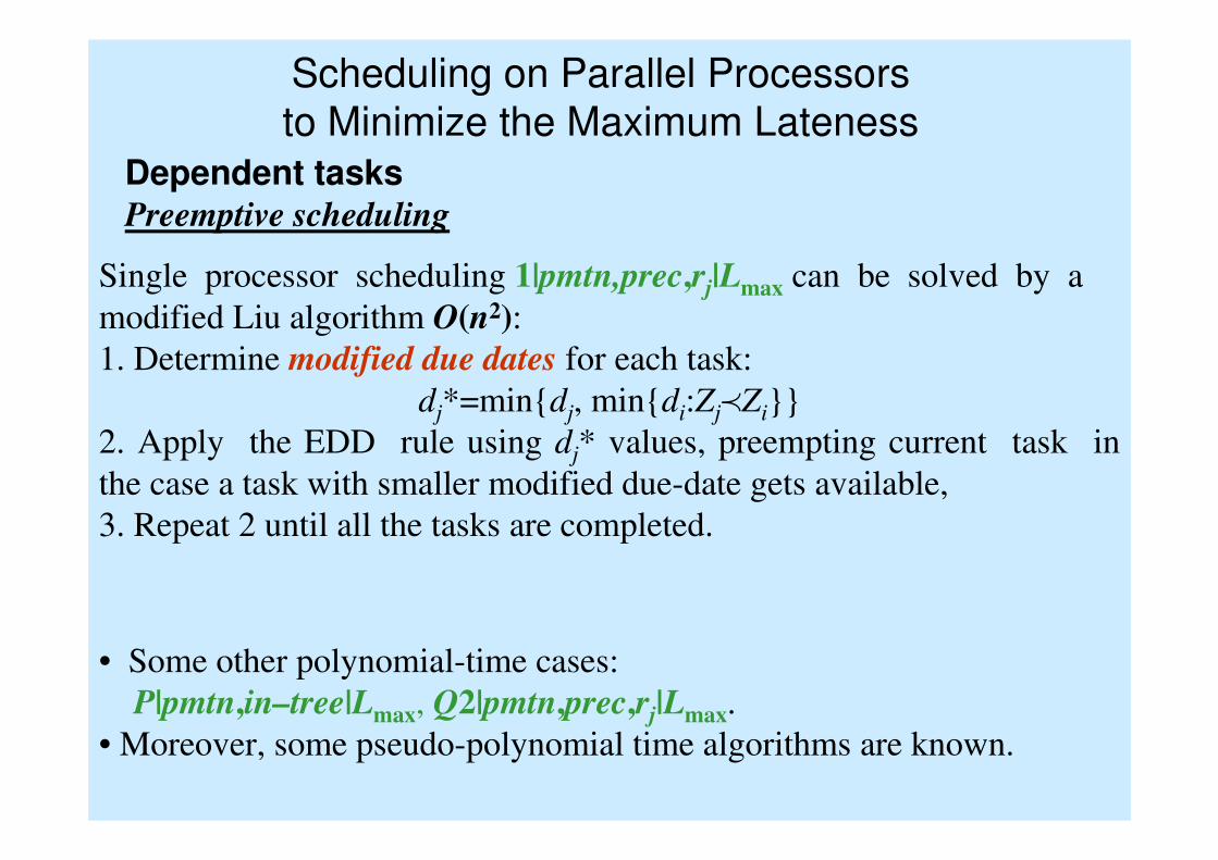
Single processor scheduling 1|pmtn,prec,rj|Lmax can be solved by a
modified Liu algorithm O(n2):
1. Determine modified due dates for each task:
dj*=min{dj, min{di:ZjpZi}}
2. Apply the EDD rule using dj* values, preempting current task in
the case a task with smaller modified due-date gets available,
3. Repeat 2 until all the tasks are completed.
Dependent tasksPreemptive scheduling
• Some other polynomial-time cases:
P|pmtn,in–tree|Lmax, Q2|pmtn,prec,rj|Lmax.
• Moreover, some pseudo-polynomial time algorithms are known.
Scheduling on Parallel Processors
to Minimize the Maximum Lateness
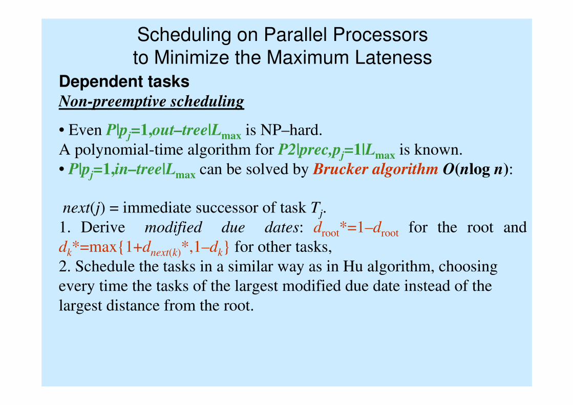
• Even P|pj=1,out–tree|Lmax is NP–hard.
A polynomial-time algorithm for P2|prec,pj=1|Lmax is known.
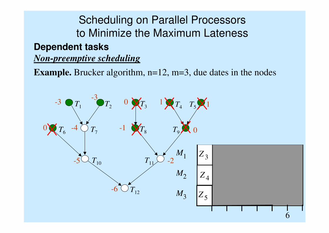
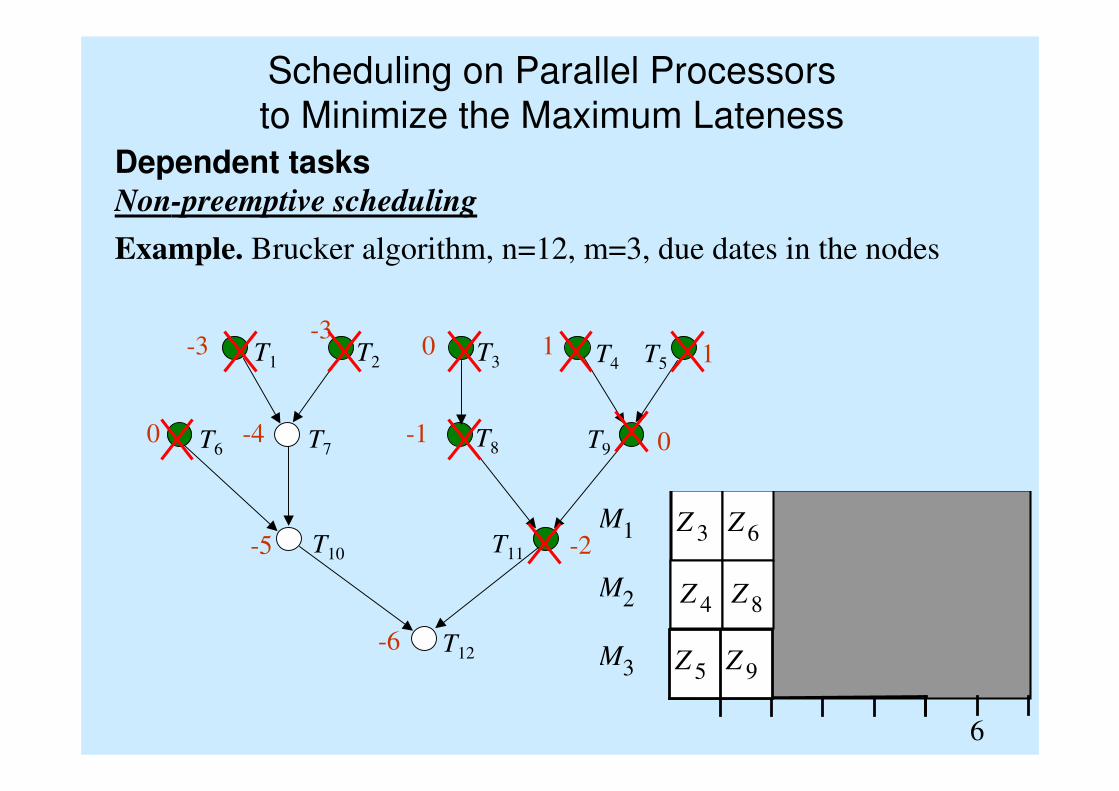
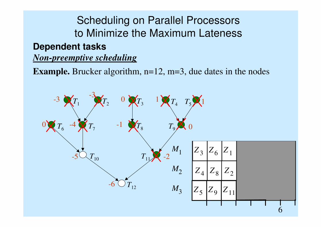
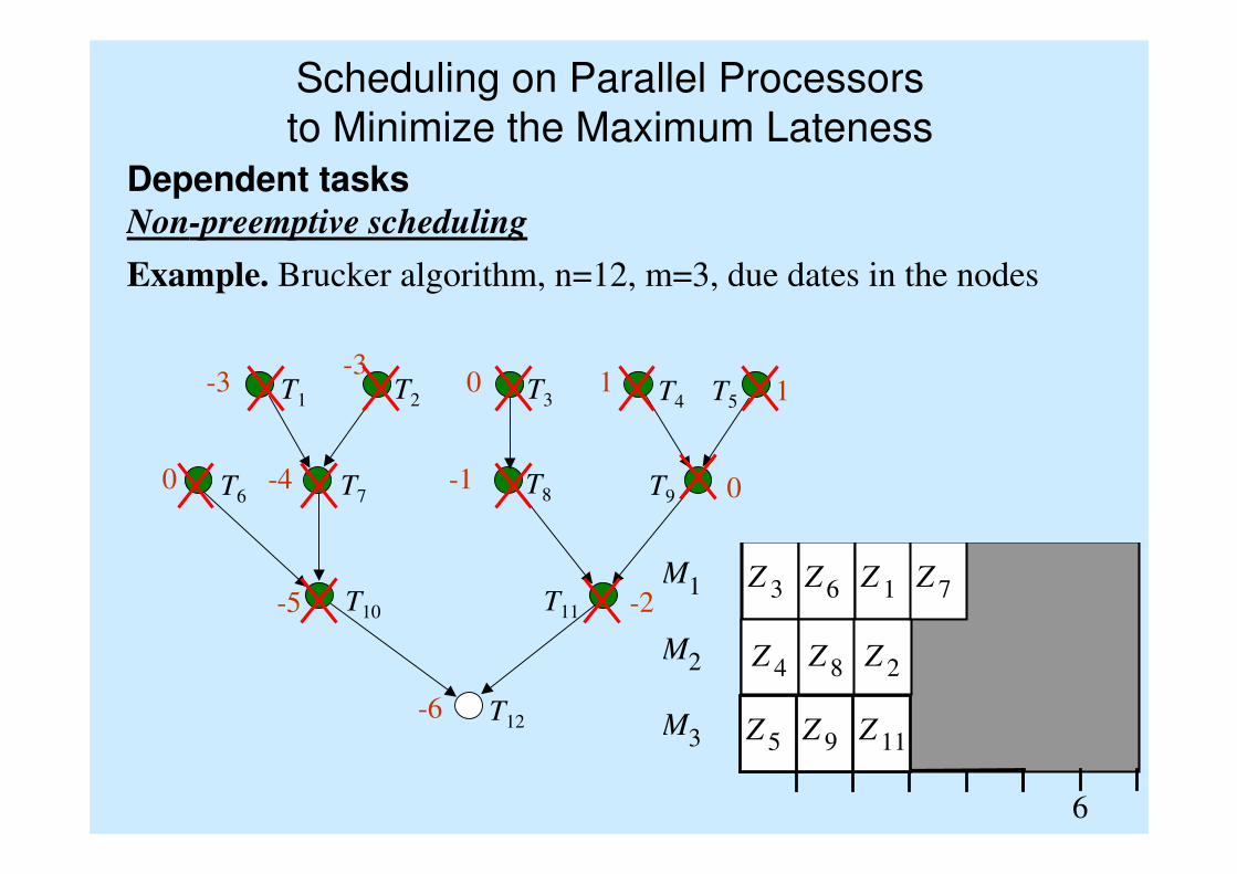
• P|pj=1,in–tree|Lmax can be solved by Brucker algorithm O(nlog n):
Dependent tasksNon-preemptive scheduling
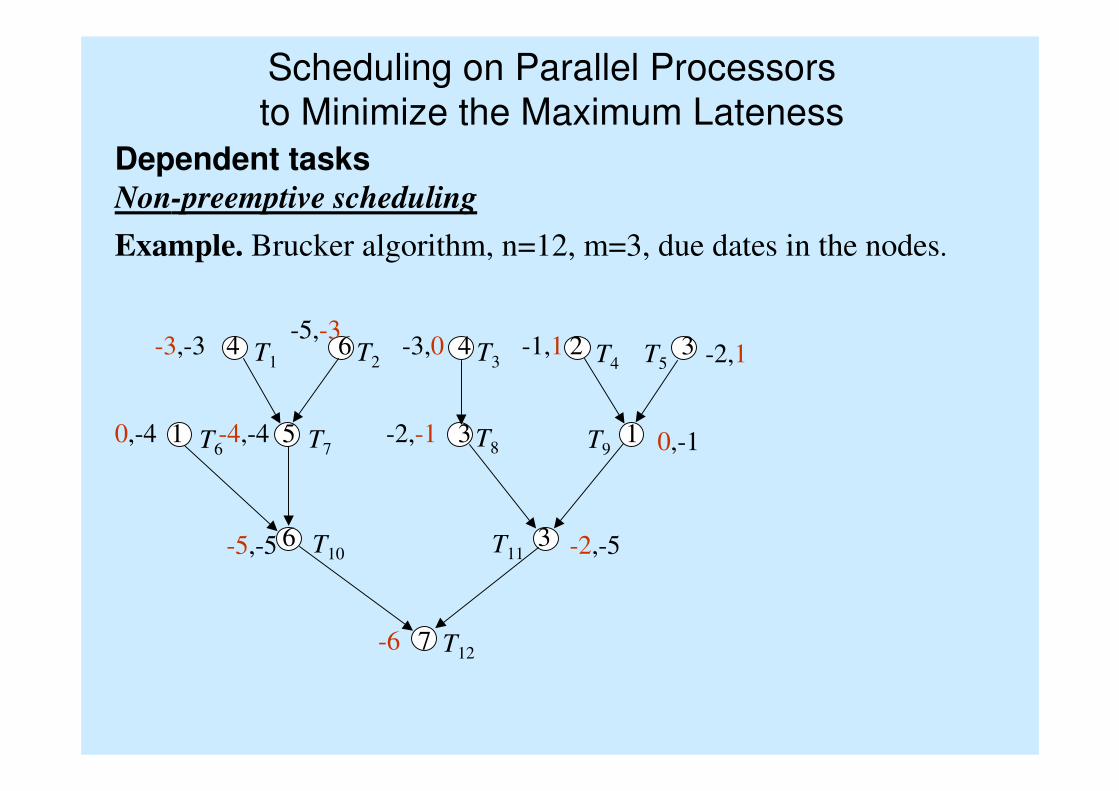
next(j) = immediate successor of task Tj.
1. Derive modified due dates: droot*=1–droot for the root and
dk*=max{1+dnext(k)*,1–dk} for other tasks,
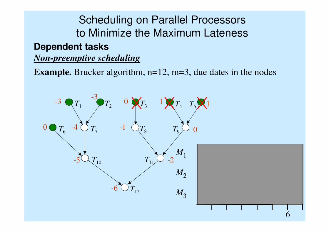
2. Schedule the tasks in a similar way as in Hu algorithm, choosing
every time the tasks of the largest modified due date instead of the
largest distance from the root.
Scheduling on Parallel Processors
to Minimize the Maximum Lateness
Dependent tasksNon-preemptive scheduling
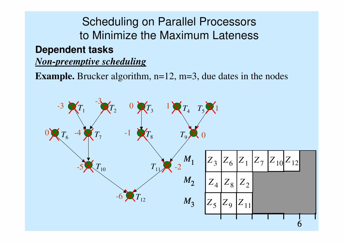
Example. Brucker algorithm, n=12, m=3, due dates in the nodes.
T1 T2 T3 T4 T5
T7T6
T10
T9T8
T11
T127
6 3
1 5 3 1
4 6 4 2 3
-6
-5,-5 -2,-5
0,-4 -4,-4 -2,-1 0,-1
-3,-3-5,-3
-3,0 -1,1 -2,1

Scheduling on Parallel Processors
to Minimize the Maximum Lateness
Dependent tasksNon-preemptive scheduling
Example. Brucker algorithm, n=12, m=3, due dates in the nodes
T1 T2 T3 T4 T5
T7T6
T10
T9T8
T11
T127
6 3
1 5 3 1
4 6 4 2 3
-6
-5 -2
0 -4 -1 0
-3 -3
0 1 1
T1 T2 T3 T4 T5
T7T6
T10
T9T8
T11
T12
M 1
M 2
M 3
6
Scheduling on Parallel Processors
to Minimize the Maximum Lateness
Dependent tasksNon-preemptive scheduling
Example. Brucker algorithm, n=12, m=3, due dates in the nodes
-6
-5 -2
0 -4 -1 0
-3 -3
0 1 1
T1 T2 T3 T4 T5
T7T6
T10
T9T8
T11
T12
M 1
M 2
M 3
6
Z 3
Z 5
Z 4
-6
-5 -2
0 -4 -1 0
-3 -3
0 1 1
Scheduling on Parallel Processors
to Minimize the Maximum Lateness
Dependent tasksNon-preemptive scheduling
Example. Brucker algorithm, n=12, m=3, due dates in the nodes
T1 T2 T3 T4 T5
T7T6
T10
T9T8
T11
T12
M 1
M 2
M 3
6
Z 3
Z 5
Z 4
Z 6
Z 9
Z 8
-6
-5 -2
0 -4 -1 0
-3 -3
0 1 1
Scheduling on Parallel Processors
to Minimize the Maximum Lateness
Dependent tasksNon-preemptive scheduling
Example. Brucker algorithm, n=12, m=3, due dates in the nodes
T1 T2 T3 T4 T5
T7T6
T10
T9T8
T11
T12
M 1
M 2
M 3
6
Z 3
Z 5
Z 4
Z 6
Z 9
Z 8
Z 1
Z 11
Z 2
-6
-5 -2
0 -4 -1 0
-3 -3
0 1 1
Scheduling on Parallel Processors
to Minimize the Maximum Lateness
Dependent tasksNon-preemptive scheduling
Example. Brucker algorithm, n=12, m=3, due dates in the nodes
T1 T2 T3 T4 T5
T7T6
T10
T9T8
T11
T12
M 1
M 2
M 3
6
Z 3
Z 5
Z 4
Z 6
Z 9
Z 8
Z 1
Z 11
Z 2
Z 7
-6
-5 -2
0 -4 -1 0
-3 -3
0 1 1
Scheduling on Parallel Processors
to Minimize the Maximum Lateness
Dependent tasksNon-preemptive scheduling
Example. Brucker algorithm, n=12, m=3, due dates in the nodes
T1 T2 T3 T4 T5
T7T6
T10
T9T8
T11
T12
M 1
M 2
M 3
6
Z 3
Z 5
Z 4
Z 6
Z 9
Z 8
Z 1
Z 11
Z 2
Z 7 Z 10
-6
-5 -2
0 -4 -1 0
-3 -3
0 1 1
Scheduling on Parallel Processors
to Minimize the Maximum Lateness
Dependent tasksNon-preemptive scheduling
Example. Brucker algorithm, n=12, m=3, due dates in the nodes
M 1
M 2
M 3
6
Z 3
Z 5
Z 4
Z 6
Z 9
Z 8
Z 1
Z 11
Z 2
Z 7 Z 10 Z 12
Scheduling on Parallel Processors
to Minimize the Maximum Lateness
Dependent tasksNon-preemptive scheduling
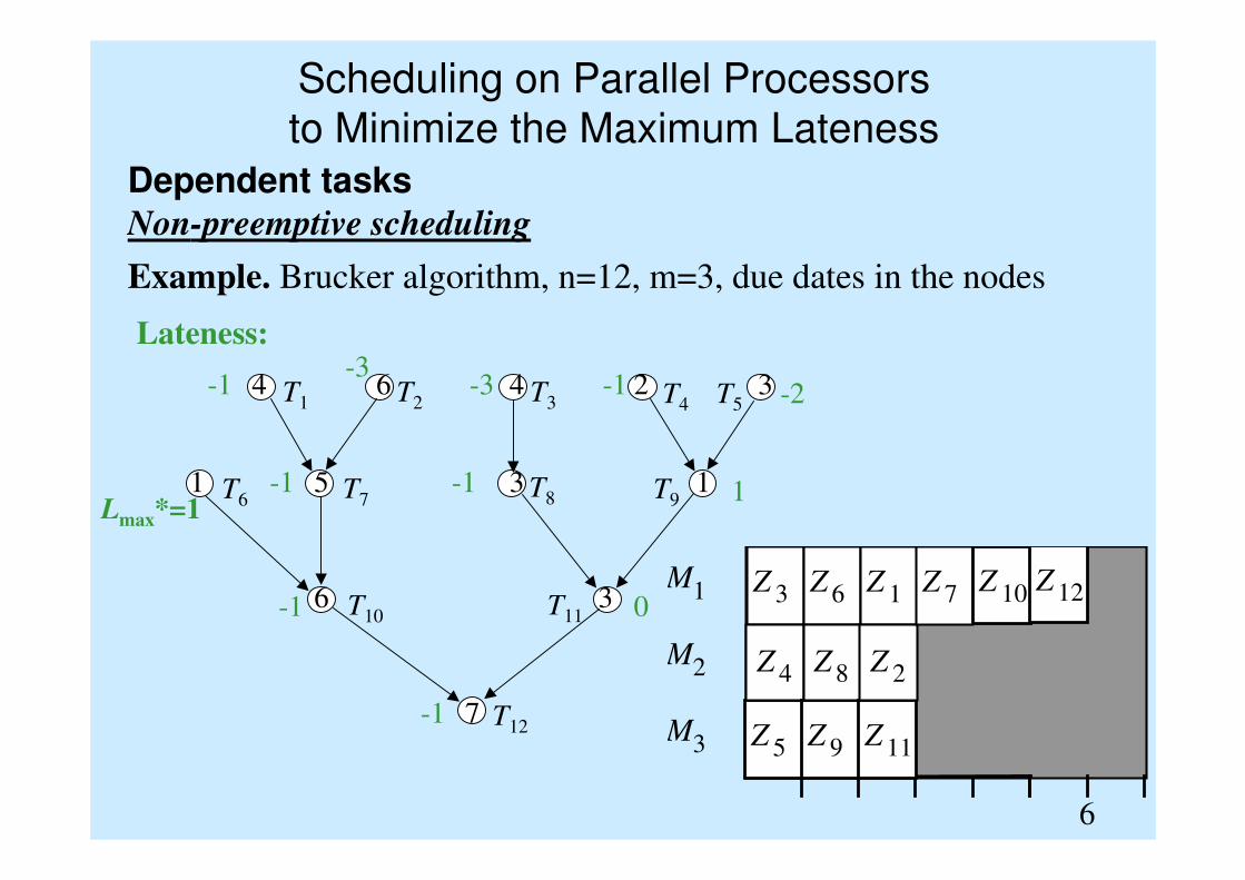
Example. Brucker algorithm, n=12, m=3, due dates in the nodes
T1 T2 T3 T4 T5
T7T6
T10
T9T8
T11
T127
6 3
1 5 3 1
4 6 4 2 3
M 1
M 2
M 3
6
Z 3
Z 5
Z 4
Z 6
Z 9
Z 8
Z 1
Z 11
Z 2
Z 7 Z 10 Z 12
-1
-1 0
Lmax*=1-1 -1 1
-1 -3
-3 -1 -2
Lateness:
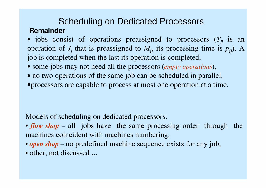
Scheduling on Dedicated ProcessorsRemainder
• jobs consist of operations preassigned to processors (Tjj is an
operation of Jj that is preassigned to Mi, its processing time is pij). A
job is completed when the last its operation is completed,
• some jobs may not need all the processors (empty operations),
• no two operations of the same job can be scheduled in parallel,
•processors are capable to process at most one operation at a time.
Models of scheduling on dedicated processors:
• flow shop – all jobs have the same processing order through the
machines coincident with machines numbering,
• open shop – no predefined machine sequence exists for any job,
• other, not discussed ...
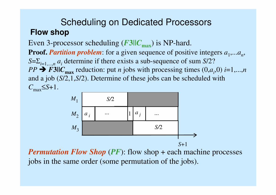
Scheduling on Dedicated ProcessorsFlow shop
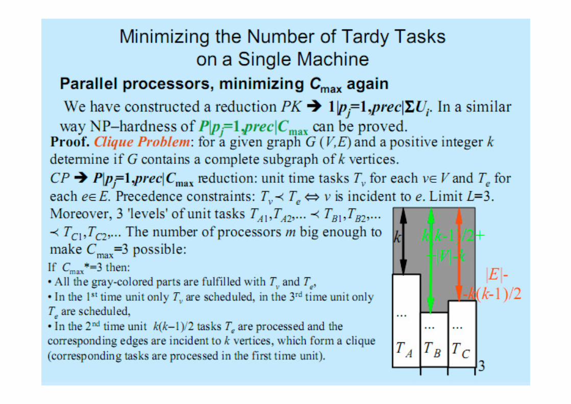
Even 3-processor scheduling (F3||Cmax) is NP-hard.
Proof. Partition problem: for a given sequence of positive integers a1,...an,
S=Σi=1,...,n ai determine if there exists a sub-sequence of sum S/2?
PP � F3||Cmax reduction: put n jobs with processing times (0,ai,0) i=1,...,n
and a job (S/2,1,S/2). Determine of these jobs can be scheduled with
Cmax≤S+1.
M1
M2
S+1
a i... a j ...
S/2
S/2
1
M3
Permutation Flow Shop (PF): flow shop + each machine processes
jobs in the same order (some permutation of the jobs).
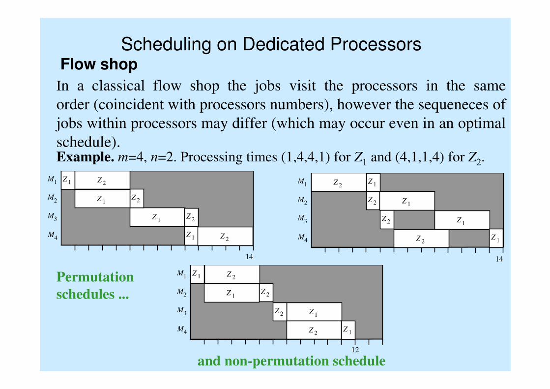
Scheduling on Dedicated ProcessorsFlow shop
In a classical flow shop the jobs visit the processors in the same
order (coincident with processors numbers), however the sequeneces of
jobs within processors may differ (which may occur even in an optimal
schedule).Example. m=4, n=2. Processing times (1,4,4,1) for Z1 and (4,1,1,4) for Z2.
M 1
M 2
M 3
14
Z 1
Z 1
M 4 Z 1
Z 2
Z 2
Z 1
Z 2
Z 2
M1
M2
M3
14
Z 1
Z 1
M4Z 1
Z 2
Z 2
Z 1
Z 2
Z 2
Permutation
schedules ...
M1
M2
M3
12
Z 1
Z 1
M4 Z 1
Z 2
Z 2
Z 1
Z 2
Z 2
and non-permutation schedule
Scheduling on Dedicated ProcessorsFlow shop
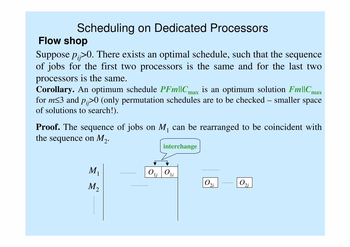
Suppose pij>0. There exists an optimal schedule, such that the sequence
of jobs for the first two processors is the same and for the last two
processors is the same.Corollary. An optimum schedule PFm||Cmax is an optimum solution Fm||Cmax
for m≤3 and pij>0 (only permutation schedules are to be checked – smaller space
of solutions to search!).
Proof. The sequence of jobs on M1 can be rearranged to be coincident with
the sequence on M2.
M1
M2
O1j O1i
O2i O2j
interchange
Scheduling on Dedicated ProcessorsFlow shop
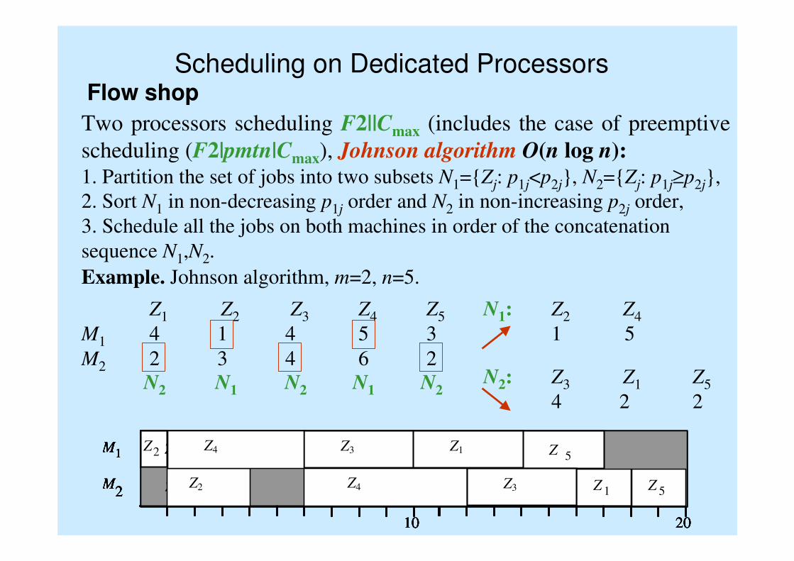
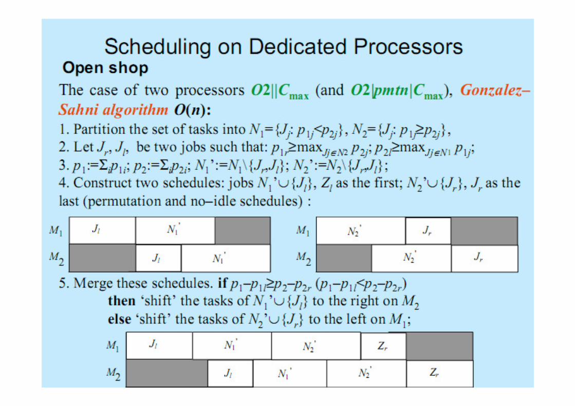
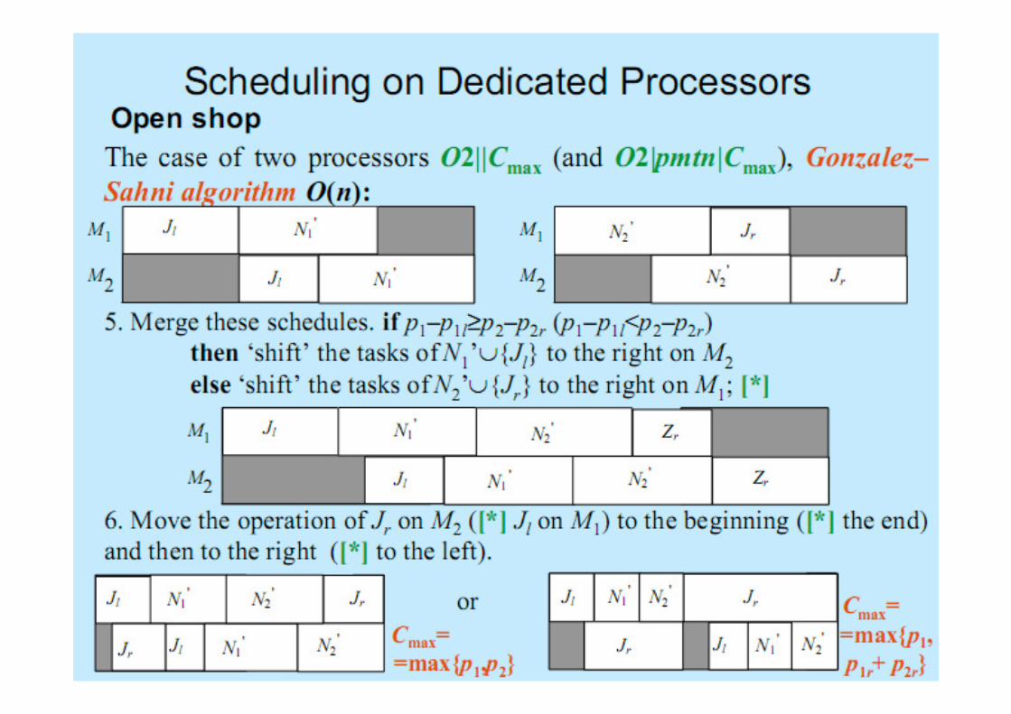
Two processors scheduling F2||Cmax (includes the case of preemptive
scheduling (F2|pmtn|Cmax), Johnson algorithm O(n log n):
1. Partition the set of jobs into two subsets N1={Zj: p1j<p2j}, N2={Zj: p1j≥p2j},
2. Sort N1 in non-decreasing p1j order and N2 in non-increasing p2j order,
3. Schedule all the jobs on both machines in order of the concatenation
sequence N1,N2.
M 1
M 2
10
Z 1 Z2
Z 2
20
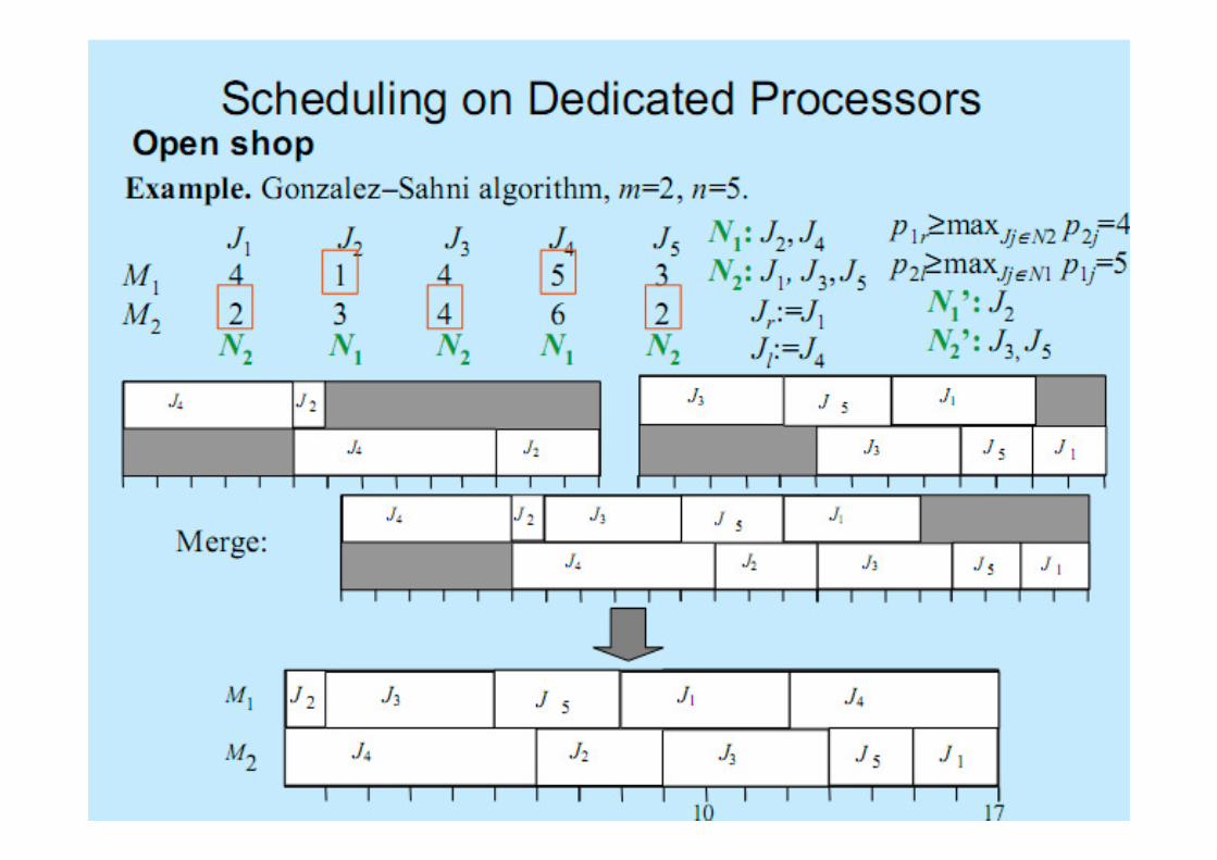
Example. Johnson algorithm, m=2, n=5.
Z1 Z2 Z3 Z4 Z5
M1 4 1 4 5 3
M2 2 3 4 6 2
N2 N1 N2 N1 N2
N1: Z2 Z4
1 5
N2: Z3 Z1 Z5
4 2 2
M 1
M 2
10
Z 1 Z2
Z 2
20
Z 1 Z4
1 Z4
M 1
M 2
10
Z 1 Z2
Z 2 Z3
20
Z 1 Z4
1 Z4 Z3
M 1
M 2
10
Z 1 Z2 Z 1
Z 2 Z3
20
Z 1 Z4
1 Z4 Z3
Z1 M 1
M 2
10
Z 5
Z 1 Z2 Z 1
Z 2 Z3
20
Z 1 Z4
1 Z4 Z3
Z1
Z 5
Scheduling on Dedicated ProcessorsFlow shop
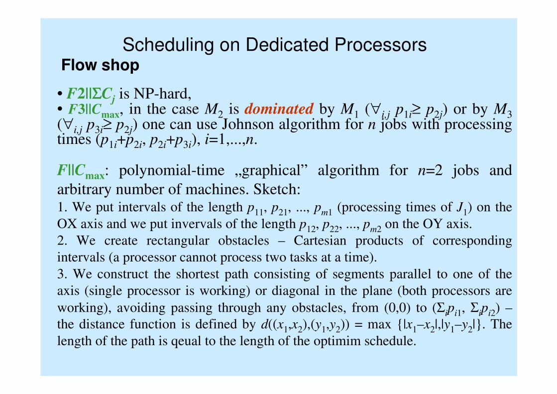
F||Cmax: polynomial-time „graphical” algorithm for n=2 jobs and
arbitrary number of machines. Sketch:1. We put intervals of the length p11, p21, ..., pm1 (processing times of J1) on the
OX axis and we put invervals of the length p12, p22, ..., pm2 on the OY axis.
2. We create rectangular obstacles – Cartesian products of corresponding
intervals (a processor cannot process two tasks at a time).
3. We construct the shortest path consisting of segments parallel to one of the
axis (single processor is working) or diagonal in the plane (both processors are
working), avoiding passing through any obstacles, from (0,0) to (Σipi1, Σipi2) –
the distance function is defined by d((x1,x2),(y1,y2)) = max {|x1–x2|,|y1–y2|}. The
length of the path is qeual to the length of the optimim schedule.
• F2||ΣΣΣΣCj is NP-hard,• F3||Cmax, in the case M2 is dominated by M1 (∀i,j p1i≥ p2j) or by M3(∀i,j p3i≥ p2j) one can use Johnson algorithm for n jobs with processingtimes (p1i+p2i, p2i+p3i), i=1,...,n.
Scheduling on Dedicated ProcessorsFlow shop
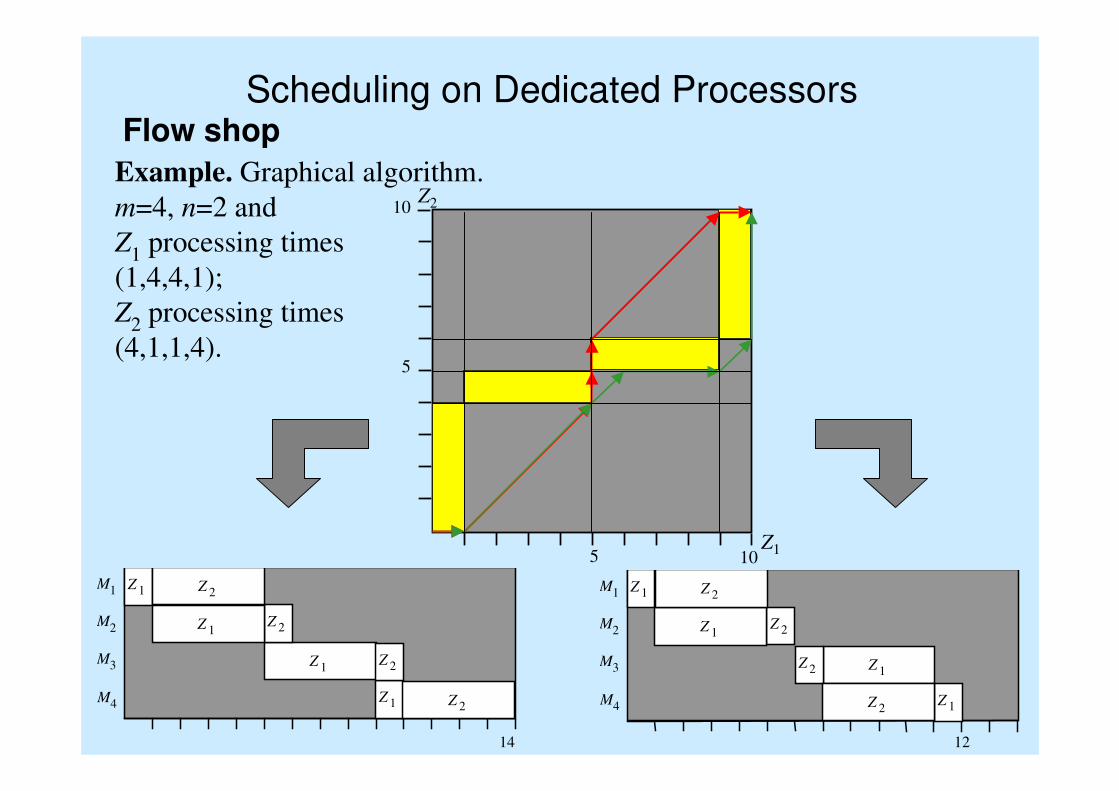
Example. Graphical algorithm.
m=4, n=2 and
Z1 processing times
(1,4,4,1);
Z2 processing times
(4,1,1,4).
M1
M2
M3
12
Z 1
Z 1
M4 Z 1
Z 2
Z 2
Z 1
Z 2
Z 2
10 5
10
5
M1
M2
M3
14
Z 1
Z 1
M4Z 1
Z 2
Z 2
Z 1
Z 2
Z 2
Z2
Z1
Scheduling on Dedicated ProcessorsOpen shop
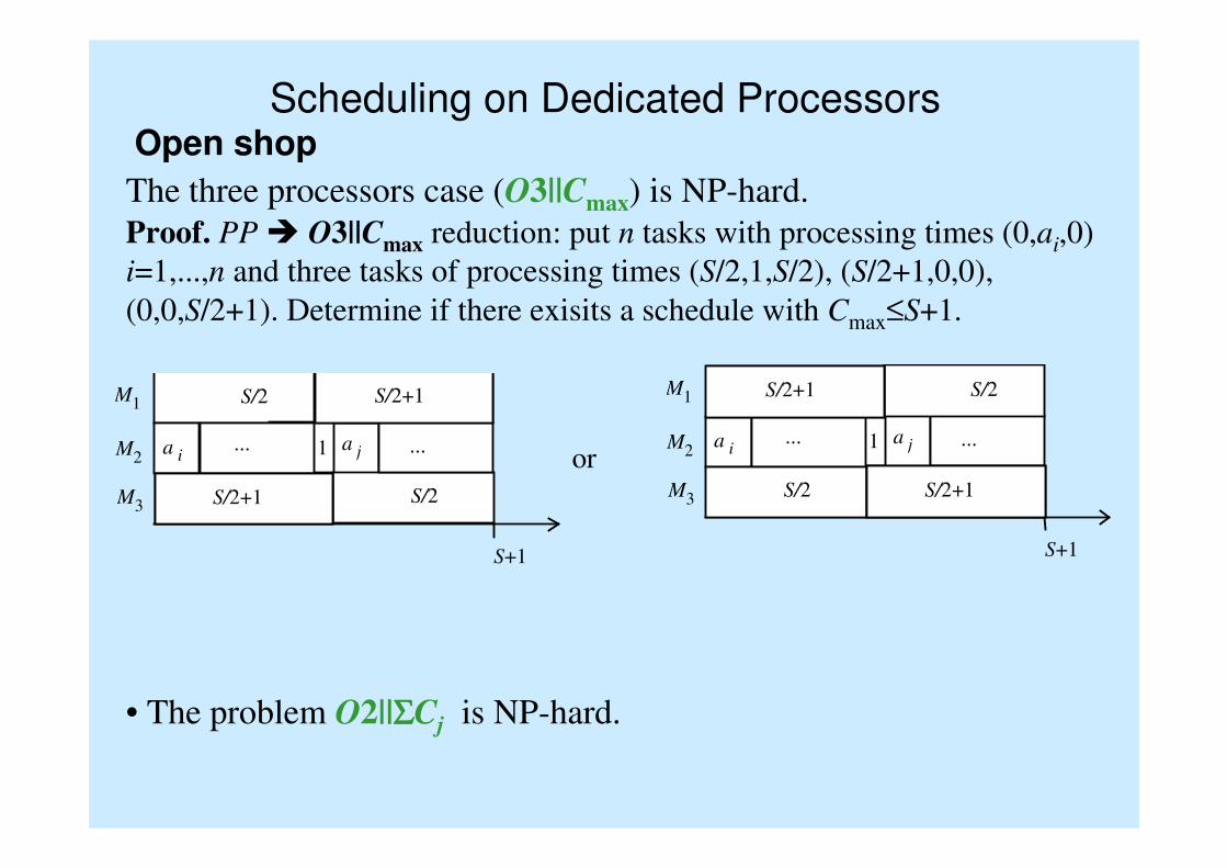
The three processors case (O3||Cmax) is NP-hard.
• The problem O2||ΣΣΣΣCj is NP-hard.
Proof. PP � O3||Cmax reduction: put n tasks with processing times (0,ai,0)
i=1,...,n and three tasks of processing times (S/2,1,S/2), (S/2+1,0,0),
(0,0,S/2+1). Determine if there exisits a schedule with Cmax≤S+1.
M1
M2
S+1
a i... a j ...
S/2
S/2
1
M3
S/2+1
S/2+1
M 1
M 2
S+1
a i ... a j ...
S/2
S/2
1
M 3
S/2+1
S/2+1
or
Scheduling on Dedicated ProcessorsOpen shop
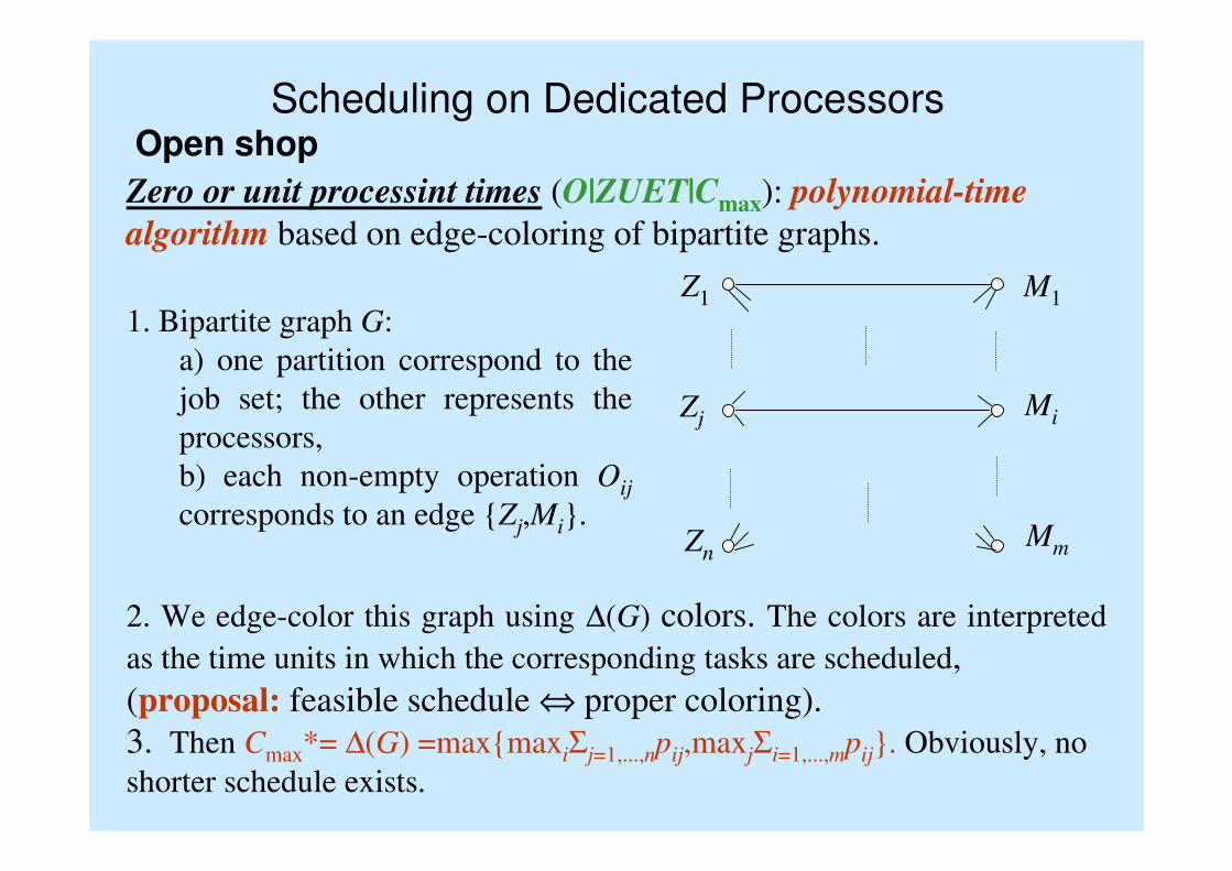
Zero or unit processint times (O|ZUET|Cmax): polynomial-time
algorithm based on edge-coloring of bipartite graphs.
M1
Zj
Zn
Mi
Mm
Z1
1. Bipartite graph G:
a) one partition correspond to the
job set; the other represents the
processors,
b) each non-empty operation Oij
corresponds to an edge {Zj,Mi}.
2. We edge-color this graph using ∆(G) colors. The colors are interpreted
as the time units in which the corresponding tasks are scheduled,
(proposal: feasible schedule ⇔ proper coloring).
3. Then Cmax*= ∆(G) =max{maxiΣj=1,...,npij,maxjΣi=1,...,mpij}. Obviously, no
shorter schedule exists.
Scheduling on Dedicated ProcessorsOpen shop
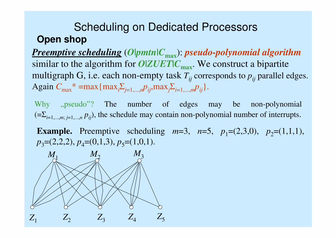
Preemptive scheduling (O|pmtn|Cmax): pseudo-polynomial algorithm
similar to the algorithm for O|ZUET|Cmax. We construct a bipartite
multigraph G, i.e. each non-empty task Tij corresponds to pij parallel edges.
Again Cmax* =max{maxiΣj=1,...,npij,maxjΣi=1,...,mpij}.
Example. Preemptive scheduling m=3, n=5, p1=(2,3,0), p2=(1,1,1),
p3=(2,2,2), p4=(0,1,3), p5=(1,0,1).
M1M2
M3
Z1Z2 Z3 Z4
Z5
Why „pseudo”? The number of edges may be non-polynomial
(=Σi=1,...,m; j=1,...,n pij), the schedule may contain non-polynomial number of interrupts.
Scheduling on Dedicated ProcessorsOpen shop
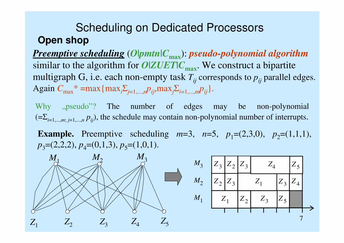
Preemptive scheduling (O|pmtn|Cmax): pseudo-polynomial algorithm
similar to the algorithm for O|ZUET|Cmax. We construct a bipartite
multigraph G, i.e. each non-empty task Tij corresponds to pij parallel edges.
Again Cmax* =max{maxiΣj=1,...,npij,maxjΣi=1,...,mpij}.
Example. Preemptive scheduling m=3, n=5, p1=(2,3,0), p2=(1,1,1),
p3=(2,2,2), p4=(0,1,3), p5=(1,0,1).
M1M2
M3
Z1Z2 Z3 Z4
Z5
Why „pseudo”? The number of edges may be non-polynomial
(=Σi=1,...,m; j=1,...,n pij), the schedule may contain non-polynomial number of interrupts.
M 3
M 2
M 1
7
Z 2
Z 3
Z 2
Z 3
Z 3
Z 2
Z 3 Z 4
Z 5
Z 5
Z 1 Z 3
Z 1
Z 4
Scheduling on Dedicated ProcessorsOpen shop
Preemptive scheduling (O|pmtn|Cmax):
• polynomial time algorithm is known; it is based on fractional edge-coloring
of weighted graph (each task Tij corresponds to an edge {Jj,Mi} of weight pij in
graph G),
Minimizing Cmax on parallel processors ... again
Polynomial-time algorithm for R|pmtn|Cmax.R|pmtn|Cmax � O|pmtn|Cmax. reduction: Let xij be the part of Tj processed by
Mi (in the time tij= pijxij). If we knew optimal values xij, we could use the
above algorithm treating these tasks’ parts as tasks of preemptive jobs
(constraints for the schedule are the same!).
How to derive these values? We transform the scheduling problem to linear
programming:
minimize C such that:
Σi=1,...,m
xij=1, j=1,...,n
C≥Σj=1,...,n
pijx
ij, i=1,...,m, C≥Σ
i=1,...,m p
ijx
ij, j=1,...,n.

![Polynomial time deterministic identity testing algorithm for … · 2020. 6. 16. · Polynomial time deterministic identity testing algorithm for S[3]PSP[2] circuits via Edelstein-Kelly](https://static.fdocument.org/doc/165x107/6149c34c12c9616cbc68f918/polynomial-time-deterministic-identity-testing-algorithm-for-2020-6-16-polynomial.jpg)