
Detection of threshold crossings in the leaky
63
1
Transcript of Detection of threshold crossings in the leaky

1

Detection of threshold crossings in the leakyintegrate-and-fire neuron model with α-shapedpostsynaptic currents in time-driven simulations
German Research School for Simulation Sciences
Master’s ThesisJeyashree Krishnan
Dr.Edoardo Di NapoliCo-Examiner
Prof.Dr.Markus DiesmannExaminer
Dr.Moritz Helias
Supervisor
Thursday 16th October, 2014
communicated by Univ.-Prof. Marek Behr

Contents
1 Introduction 7
2 Subthreshold dynamics in time-driven simulations 11
3 Determination of peak time using Lambert W function 193.1 Lambert W function . . . . . . . . . . . . . . . . . . . . . . . . . . . . . . . . . . . . 193.2 Peak time of PSP . . . . . . . . . . . . . . . . . . . . . . . . . . . . . . . . . . . . . . 203.3 Critical conditions . . . . . . . . . . . . . . . . . . . . . . . . . . . . . . . . . . . . . 27
3.3.1 Initial condition y1(0) = 0 . . . . . . . . . . . . . . . . . . . . . . . . . . . 273.3.2 Real-valued solution of the Lambert W function . . . . . . . . . . . . . . 28
4 Continuous-time spiking neuron models 314.1 NEST . . . . . . . . . . . . . . . . . . . . . . . . . . . . . . . . . . . . . . . . . . . . . 314.2 α− neuron model . . . . . . . . . . . . . . . . . . . . . . . . . . . . . . . . . . . . . 314.3 Spike test . . . . . . . . . . . . . . . . . . . . . . . . . . . . . . . . . . . . . . . . . . 394.4 Neuron embedded in a quasi-network setup . . . . . . . . . . . . . . . . . . . . . 434.5 Efficiency of spike test . . . . . . . . . . . . . . . . . . . . . . . . . . . . . . . . . . 49
5 Discussion 59
5

1 Introduction
Neuroscience is the scientific study of the nervous system that attempts to understand infor-mation processing in the brain in terms of electrical activity in different parts of the centralnervous system. A neuron, the functional unit of the nervous system, is an electrically ex-citable cell that processes and transmits information through electrical and chemical signalsvia the points of contacts, called synapses. The brain is a complex system with high connec-tivity. Neural systems are nonlinear and stochastic in nature. Experimental data to studysuch a system is only available either for single or extremely small numbers of neuronsor for superposition signals from very large populations, necessitating the application oftheoretical and computational methods to understand the dynamic properties of neurons.Therefore, neural network simulations are crucial for the advancement of brain research.
Computational neuroscience is the study of brain function using theoretical methods andcomputer simulations. Simulations of neurons employ mathematical models to focus onreproducing the neural activity in the brain. The dynamics of a neuron can be described bya set of differential equations where the interaction between a pair of neurons is simulatedas point events, i.e. spikes. The spike or action potential is the unit of signal transmission.A typical neuron possesses a cell body, dendrites, and an axon. The dendrites act as inputdevices and collect input signals from other neurons and transmit them to the soma. Thecell body can be considered as the central processing unit that performs a non-linear pro-cessing step i.e. if the input exceeds a certain threshold voltage then a spike occurs. Theaxon or the output device delivers the output signal to other neurons. By convention, thesending neuron is referred to as the presynaptic cell and the receiving neuron as the postsy-naptic cell. A spike causes a small change in the membrane potential of the target neurons,called the postsynaptic potential (PSP). These PSPs can then further initiate or inhibit actionpotentials.
The membrane potential can be static, in absence of inputs, or dynamic, if the cell receivessynaptic input. When synaptic inputs are absent, the membrane potential of the neuronassumes a static value, called the resting voltage. This potential difference between theinterior and exterior of a neuron is determined by differences of ionic concentrations insideand outside the cell body, that are kept up by active transport mechanisms.
Two common approaches to modeling the nervous system are the top-down and bottom-up approaches. In the bottom-up approach neuron are considered as nodes and their synap-tic connections as edges. The network can then be described in terms of the neurons, andtheir projections. This approach is referred to as bottom-up, since we construct the networkfrom its basic components, the neurons. Hence there are simulation tools, techniques forsingle or small numbers of neurons that focus on their morphology and function, like theNEURON simulator [Hines, 1993], and simulation tools to study large networks of simplecells, like SPLIT [Djurfeldt, 2009], the Brian simulator [Goodman and Brette, 2009], the
7
1 Introduction
C2 simulator [Ananthanarayanan and Modha, 2007], and NEST [Gewaltig and Diesmann,2007]. In a top-down approach, an algorithm described at an abstract mathematical levelis implemented using the constituents available in a neuronal network, i.e. neurons andsynapses.
Simplified neuron models that neglect the morphological structure of the individual cells,enables the simulation of a large number of neurons while maintaining an acceptable degreeof biological detail [Diesmann and Gewaltig, 2002]. Neural network simulators are softwareapplications that are used to simulate the behavior of artificial or biological neural networks.NEST is a simulator for networks of point neurons, that is, neuron models that collapse themorphology of different parts of a neuron to a single compartment or a small number ofcompartments [Gewaltig and Diesmann, 2007]. NEST considers neurons as nodes withpossibly complex connectivity and is aimed to understand the dynamics of large neuronalnetworks.
Two classical approaches to simulate neuronal networks are the time-driven and event-driven methods [Fujimoto, 2000, Zeigler et al., 2000, Sloot et al., 1999, Ferscha, 1996].Both of these methods describe the physical system in terms of a set of state variables rep-resenting the neurons and events mediate the interaction between cells. In a time-drivenalgorithm the time evolution advances the dynamics of each neuron in time steps definedby a computational step size h as illustrated in Figure 2.0.2 on page 14. The system ismonitored in unitary time intervals. The characteristics of a time-driven simulation area fixed-size simulation step and a fixed-size communication interval. The simulation stepsize determines discrete points in time when all neurons are updated and checked for theirmembrane potential to cross the threshold. The choice of this constant size is, as in anynumerical simulation, a trade-off between precision and simulation time. In the implemen-tation with precise spike timing [Morrison et al., 2007b], a variant of the time-driven ap-proach, the arrival times of incoming spikes introduce additional update-and-check points.Incoming spikes are incorporated and membrane potential crossings are detected only atthese update-and-check points. The communication interval is a multiple of the simula-tion step size and defines those discrete points where neurons communicate their spikes toother neurons. This interval can be as long as the minimum synaptic delay in the network[Morrison et al., 2005b]. If the voltage of one neuron crosses the threshold, then a spike isdelivered to each of the neurons that it is connected to. After all the neurons are updated,the next iteration begins. The simulation step can therefore be increased up to the size ofthe communication interval. The detection of a threshold crossing can only take place ata check point, but the timing of the spike is estimated with precision limited only by therepresentation of the double floating point number, ε [Kunkel et al., 2011], where ε is thesmallest number for which the double representation of 1+ ε is different from 1 [Morrisonet al., 2007b].
In the event-driven simulation, we observe the system only at points in time where spikeoccurrence or a threshold crossing is detected when a neuron receives an event. If this eventleads to a spike occurrence, then it is inserted into the queue. Future event occurrencesinduced by states have to be scheduled. Apart from the global clock and state variablesindicating the current state of the system that is also characteristic to a time-driven simu-
8
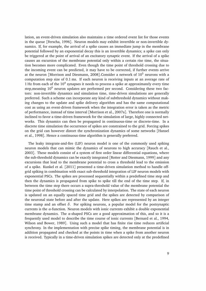
lation, an event-driven simulation also maintains a time ordered event list for those eventsin the queue [Ferscha, 1996]. Neuron models may exhibit invertible or non-invertible dy-namics. If, for example, the arrival of a spike causes an immediate jump in the membranepotential followed by an exponential decay this is an invertible dynamics; a spike can onlybe triggered at the point of arrival of an excitatory synaptic event. If the arrival of a spikecauses an excursion of the membrane potential only within a certain rise time, the situa-tion becomes more complicated. Even though the time point of threshold crossing due tothe incoming event can be predicted, it may have to be corrected, if further events arriveat the neuron [Morrison and Diesmann, 2008].Consider a network of 105 neurons with acomputation step size of 0.1 ms. If each neuron is receiving inputs at an average rate of1 Hz from each of the 104 synapses it needs to process a spike at approximately every timestep,meaning 109 neuron updates are performed per second. Considering these two fac-tors: non-invertible dynamics and simulation time, time-driven simulations are generallypreferred. Such a scheme can incorporate any kind of subthreshold dynamics without mak-ing changes to the update and spike delivery algorithm and has the same computationalcost as using an event-driven framework when the integration error is taken as the metricof performance, instead of time interval [Morrison et al., 2007a]. Therefore one is normallyinclined to favor a time-driven framework for the simulation of large, highly connected net-works. This dynamics can then be propagated in continuous-time or discrete-time. In adiscrete time simulation the occurrence of spikes are constrained to the grid. Forcing spikeson the grid can however distort the synchronization dynamics of some networks [Hanselet al., 1998]. Hence a continuous-time algorithm is generally preferred.
The leaky integrate-and-fire (LIF) neuron model is one of the commonly used spikingneuron models that can mimic the dynamics of neurons to high accuracy [Rauch et al.,2003]. These models consist of a system of first order linear differential equations, wherethe sub-threshold dynamics can be exactly integrated [Rotter and Diesmann, 1999] and anyexcursions that lead to the membrane potential to cross a threshold lead to the emissionof a spike. Kunkel et al. [2011] presented a time-driven simulation method to handle off-grid spiking in combination with exact sub-threshold integration of LIF neuron models withexponential PSCs. The spikes are processed sequentially within a predefined time step andthen the dynamics is propagated from spike to spike till the end of the time step. If, inbetween the time step there occurs a supra-threshold value of the membrane potential thetime point of threshold crossing can be calculated by interpolation. The state of each neuronis updated on an equally spaced time grid and the spikes are detected by comparison ofthe neuronal state before and after the update. Here spikes are represented by an integertime stamp and an offset δ. For spiking neurons, a popular model for the postsynapticcurrents is the α-function. Neuron models with ionic currents exhibit a double exponentialmembrane dynamics. The α-shaped PSCs are a good approximation of this, and so it is afrequently used model to describe the time course of ionic currents [Bernard et al., 1994,Wilson and Bower, 1989]. Using such a model that has finite rise time reduces artificialsynchrony. In the implementation with precise spike timing, the membrane potential is inaddition propagated and checked at the points in time when a spike from another neuronis received. Typically in a time-driven simulation spikes are detected only at the predefined
9
1 Introduction
update-and-check points. In the case of a brief membrane potential excursion a thresholdcrossing might therefore not be detected at the next check point.
Morrison et al. [2007a] developed the canonical α-model that handles events by ex-act subthreshold integration in discrete-time neural networks with continuous spike times.Hansel et al. [1998] and Shelley and Tao [2001] discuss the method of a precise simula-tion wherein the exact spike timing is calculated by interpolating the spike time within thegrid. Morrison et al. [2005a] addresses why one needs to adopt the precise spike timingapproach. In a purely on-grid scenario, the threshold crossings that occurs between twoconsecutive intervals of a time grid and would not carry a precise timestamp which maylead to artificial synchronization. In addition, grid-constrained spiking causes an integra-tion error that declines only linearly with the resolution h. The idea of the current work isto extend this existing α-model by including a spike test as implemented by Kunkel et al.[2011]. Supplementing the canonical α-model in NEST with standard tests that checks forsupra-threshold membrane potential using an algorithm that can compute the peak time ofthreshold crossing between two consecutive interval warrants that the new model (called“lossless” in the following) is a precise implementation of the mathematical definition ofthe model. The objective of this work therefore is to implement a series of tests based onthe initial and final conditions of the dynamic variables at the beginning and the end of asimulation time step that allow to detect whether or not a spike has been missed. Spikemisses can be traced back in time by expressing the peak time in terms of the Lambert Wfunction [Corless et al., 1996]. These tests determine whether the initial conditions at theleft check point and the final conditions at the right check point indicate that an excursionexceeding the threshold has happened in between. We need to find a computationally cheapand efficient implementations of the spike tests to catch the missed spikes given the typicalstatistics of input state variables. The resulting missed spike can be detected by includingthis spike-test algorithm at all check points.
10
2 Subthreshold dynamics in time-drivensimulations
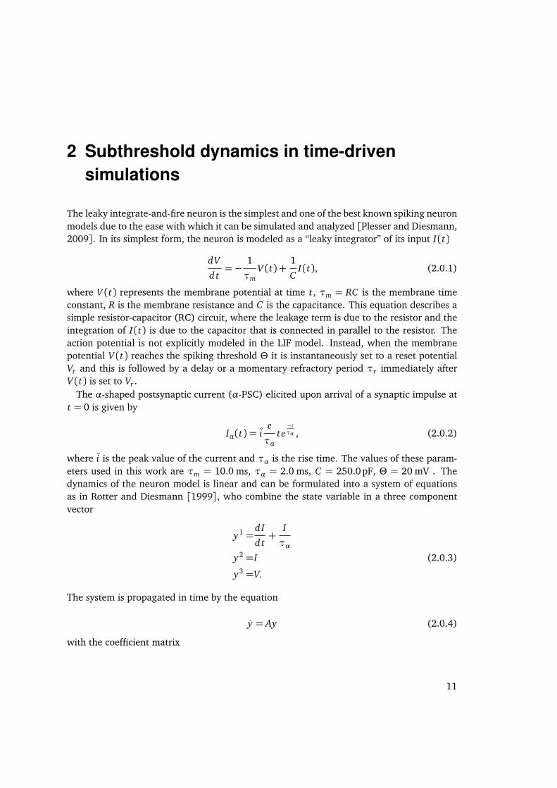
The leaky integrate-and-fire neuron is the simplest and one of the best known spiking neuronmodels due to the ease with which it can be simulated and analyzed [Plesser and Diesmann,2009]. In its simplest form, the neuron is modeled as a “leaky integrator” of its input I(t)
dV
d t=−
1
τmV (t) +
1
CI(t), (2.0.1)
where V (t) represents the membrane potential at time t, τm = RC is the membrane timeconstant, R is the membrane resistance and C is the capacitance. This equation describes asimple resistor-capacitor (RC) circuit, where the leakage term is due to the resistor and theintegration of I(t) is due to the capacitor that is connected in parallel to the resistor. Theaction potential is not explicitly modeled in the LIF model. Instead, when the membranepotential V (t) reaches the spiking threshold Θ it is instantaneously set to a reset potentialVr and this is followed by a delay or a momentary refractory period τr immediately afterV (t) is set to Vr .
The α-shaped postsynaptic current (α-PSC) elicited upon arrival of a synaptic impulse att = 0 is given by
Iα(t) = ie
ταte−tτα , (2.0.2)
where i is the peak value of the current and τα is the rise time. The values of these param-eters used in this work are τm = 10.0 ms, τα = 2.0 ms, C = 250.0pF, Θ = 20 mV . Thedynamics of the neuron model is linear and can be formulated into a system of equationsas in Rotter and Diesmann [1999], who combine the state variable in a three componentvector
y1 =dI
d t+
I
τα
y2 =I (2.0.3)
y3 =V.
The system is propagated in time by the equation
y = Ay (2.0.4)
with the coefficient matrix
11
2 Subthreshold dynamics in time-driven simulations
A=
− 1τα
0 0
1 − 1τα
0
0 1C
− 1τm
, (2.0.5)
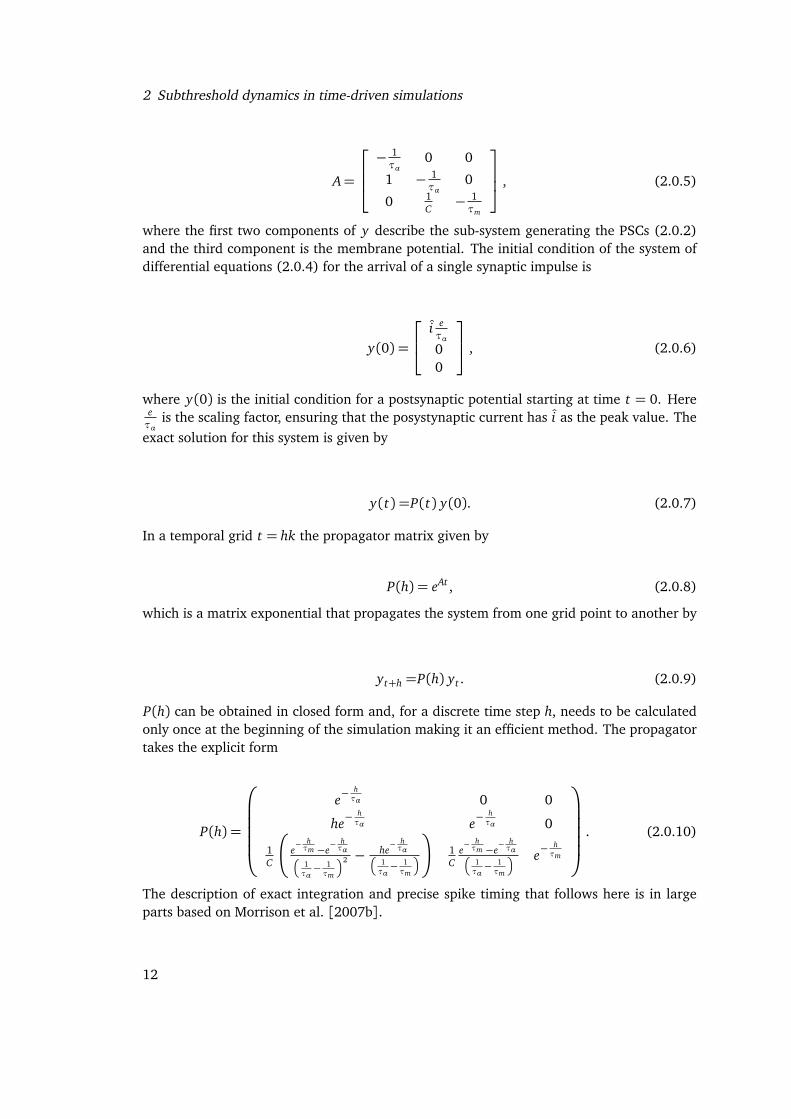
where the first two components of y describe the sub-system generating the PSCs (2.0.2)and the third component is the membrane potential. The initial condition of the system ofdifferential equations (2.0.4) for the arrival of a single synaptic impulse is
y(0) =
i eτα00
, (2.0.6)
where y(0) is the initial condition for a postsynaptic potential starting at time t = 0. Hereeτα
is the scaling factor, ensuring that the posystynaptic current has i as the peak value. Theexact solution for this system is given by
y(t) =P(t) y(0). (2.0.7)
In a temporal grid t = hk the propagator matrix given by
P(h) = eAt , (2.0.8)
which is a matrix exponential that propagates the system from one grid point to another by
yt+h =P(h) yt . (2.0.9)
P(h) can be obtained in closed form and, for a discrete time step h, needs to be calculatedonly once at the beginning of the simulation making it an efficient method. The propagatortakes the explicit form
P(h) =
e−hτα 0 0
he−hτα e−
hτα 0
1C
e− hτm −e
− hτα
�
1τα− 1τm
�2 − he− hτα
�
1τα− 1τm
�
!
1C
e− hτm −e
− hτα
�
1τα− 1τm
� e−hτm
. (2.0.10)
The description of exact integration and precise spike timing that follows here is in largeparts based on Morrison et al. [2007b].
12
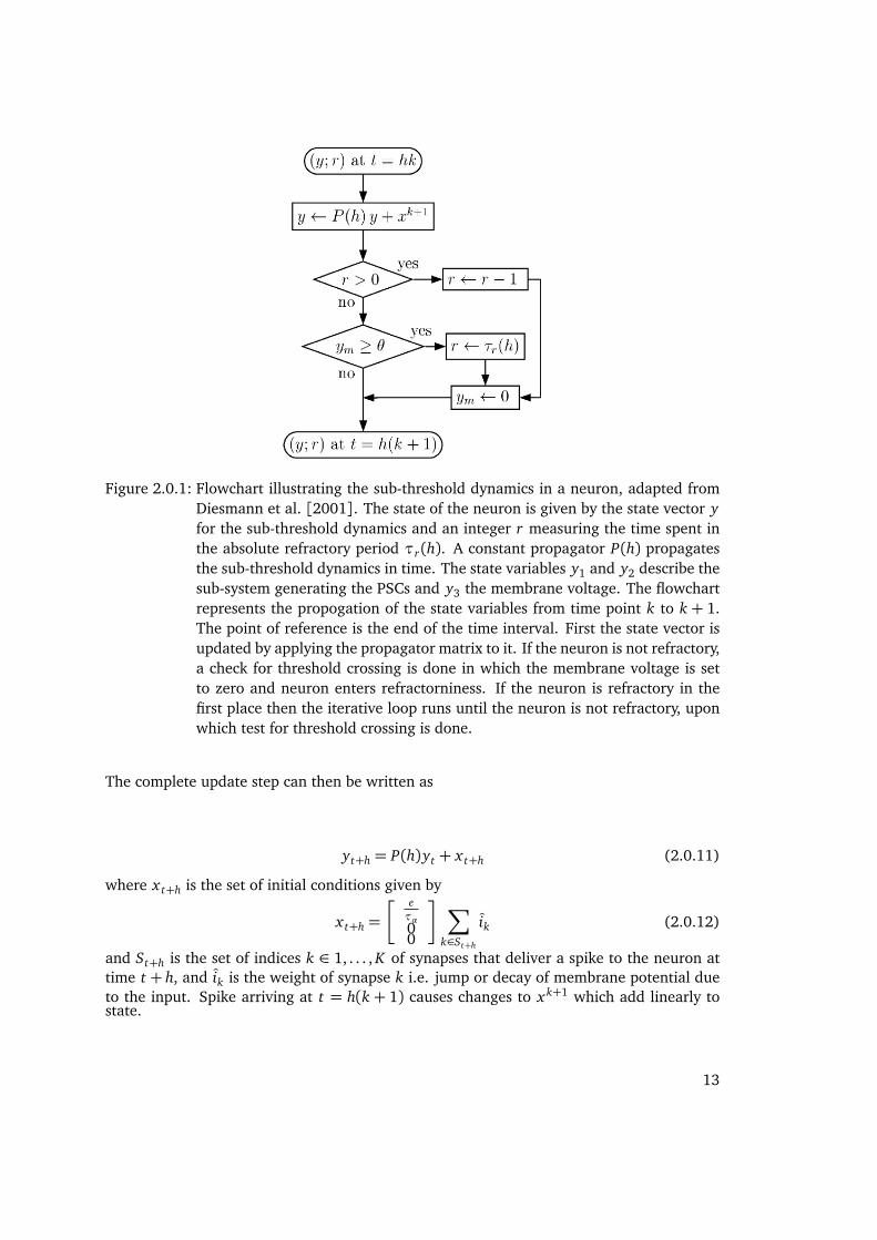
Figure 2.0.1: Flowchart illustrating the sub-threshold dynamics in a neuron, adapted fromDiesmann et al. [2001]. The state of the neuron is given by the state vector yfor the sub-threshold dynamics and an integer r measuring the time spent inthe absolute refractory period τr(h). A constant propagator P(h) propagatesthe sub-threshold dynamics in time. The state variables y1 and y2 describe thesub-system generating the PSCs and y3 the membrane voltage. The flowchartrepresents the propogation of the state variables from time point k to k + 1.The point of reference is the end of the time interval. First the state vector isupdated by applying the propagator matrix to it. If the neuron is not refractory,a check for threshold crossing is done in which the membrane voltage is setto zero and neuron enters refractorniness. If the neuron is refractory in thefirst place then the iterative loop runs until the neuron is not refractory, uponwhich test for threshold crossing is done.
The complete update step can then be written as
yt+h = P(h)yt + x t+h (2.0.11)
where x t+h is the set of initial conditions given by
x t+h =
� eτα00
�
∑
k∈St+h
ik (2.0.12)
and St+h is the set of indices k ∈ 1, . . . , K of synapses that deliver a spike to the neuron attime t + h, and ik is the weight of synapse k i.e. jump or decay of membrane potential dueto the input. Spike arriving at t = h(k + 1) causes changes to xk+1 which add linearly tostate.
13
2 Subthreshold dynamics in time-driven simulations
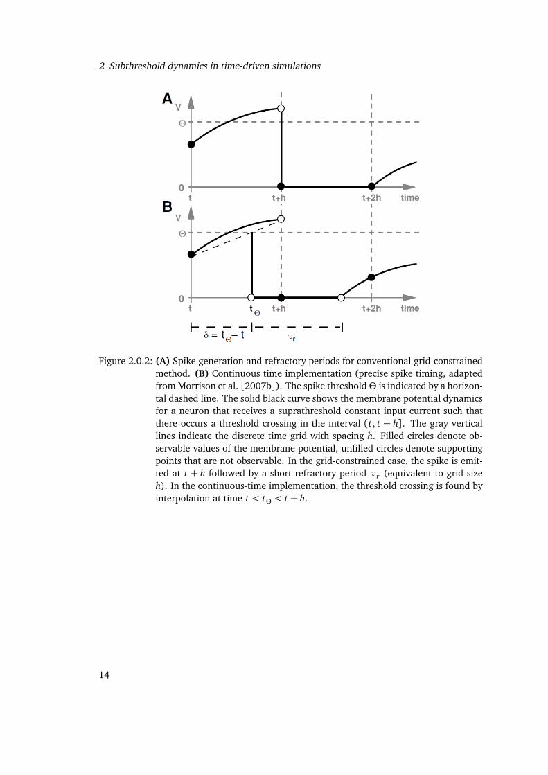
Figure 2.0.2: (A) Spike generation and refractory periods for conventional grid-constrainedmethod. (B) Continuous time implementation (precise spike timing, adaptedfrom Morrison et al. [2007b]). The spike thresholdΘ is indicated by a horizon-tal dashed line. The solid black curve shows the membrane potential dynamicsfor a neuron that receives a suprathreshold constant input current such thatthere occurs a threshold crossing in the interval (t, t + h]. The gray verticallines indicate the discrete time grid with spacing h. Filled circles denote ob-servable values of the membrane potential, unfilled circles denote supportingpoints that are not observable. In the grid-constrained case, the spike is emit-ted at t + h followed by a short refractory period τr (equivalent to grid sizeh). In the continuous-time implementation, the threshold crossing is found byinterpolation at time t < tΘ < t + h.
14
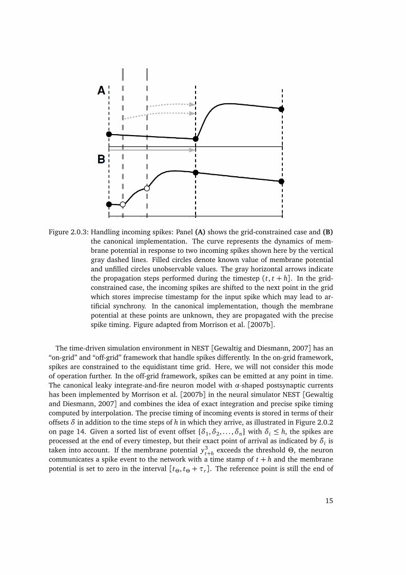
Figure 2.0.3: Handling incoming spikes: Panel (A) shows the grid-constrained case and (B)the canonical implementation. The curve represents the dynamics of mem-brane potential in response to two incoming spikes shown here by the verticalgray dashed lines. Filled circles denote known value of membrane potentialand unfilled circles unobservable values. The gray horizontal arrows indicatethe propagation steps performed during the timestep (t, t + h]. In the grid-constrained case, the incoming spikes are shifted to the next point in the gridwhich stores imprecise timestamp for the input spike which may lead to ar-tificial synchrony. In the canonical implementation, though the membranepotential at these points are unknown, they are propagated with the precisespike timing. Figure adapted from Morrison et al. [2007b].
The time-driven simulation environment in NEST [Gewaltig and Diesmann, 2007] has an“on-grid” and “off-grid” framework that handle spikes differently. In the on-grid framework,spikes are constrained to the equidistant time grid. Here, we will not consider this modeof operation further. In the off-grid framework, spikes can be emitted at any point in time.The canonical leaky integrate-and-fire neuron model with α-shaped postsynaptic currentshas been implemented by Morrison et al. [2007b] in the neural simulator NEST [Gewaltigand Diesmann, 2007] and combines the idea of exact integration and precise spike timingcomputed by interpolation. The precise timing of incoming events is stored in terms of theiroffsets δ in addition to the time steps of h in which they arrive, as illustrated in Figure 2.0.2on page 14. Given a sorted list of event offset {δ1,δ2, . . . ,δn} with δi ≤ h, the spikes areprocessed at the end of every timestep, but their exact point of arrival as indicated by δi istaken into account. If the membrane potential y3
t+h exceeds the threshold Θ, the neuroncommunicates a spike event to the network with a time stamp of t + h and the membranepotential is set to zero in the interval [tΘ, tΘ + τr]. The reference point is still the end of
15
2 Subthreshold dynamics in time-driven simulations
interval, and hence the spike emitted carries the timestamp t + h with an offset δ = tΘ− t.The neuron is then refractory from tΘ till tΘ + τr where in the membrane potential isclamped to zero and starts evolving thereafter. Given the sequence of incoming synapticevents with offsets {δ1,δ2, . . . ,δn}, the subthreshold dynamics is propagrated within onetime step of duration h from event to event, to the time point of arrival of the first event
yt+δ1=P(δ1)yt + xδ1
, (2.0.13)
to the time point of the second event
yt+δ2= P(δ2−δ1)yt+δ1
+ xδ2(2.0.14)
...
yt+δn= P(δn−δn−1)yt+δn−1
+ xδn(2.0.15)
till the end of the timestep
yt+h = P(h−δn)yt+δn. (2.0.16)
If the membrane potential of the neuron is y3t+δi
< Θ and y3t+δi+1
≥ Θ then the membranepotential of the neuron reached threshold between t +δi and t +δi+1. Since the dynamicsof the neuron is non-invertible, this threshold crossing is detected by interpolation in thecanonical model. This event now carries the timestamp t+h and an offset δ = tΘ− t. Afterspike is emitted, y3 is reset to zero and the neuron undergoes refractoriness for a durationτr .
We see that the simulation step and the arrival of synaptic events defines the update-and-check points, and the communication interval defines the discrete points in time whenall the neurons communicate their spikes. The communication interval is a multiple of thesimulation step size and is limited only by the synaptic delay in the network [Morrison andDiesmann, 2008, Kunkel et al., 2011]. Also, the simulation step size is bounded by the sizeof this communication interval. Consider a situation illustrated in Figure 2.0.4 on page 17when a short excursion of the membrane potential above threshold happens between thetwo check points and goes undetected, resulting in a missed spike.
16
θ
tleft
tright
V tmaxV
maxt}h
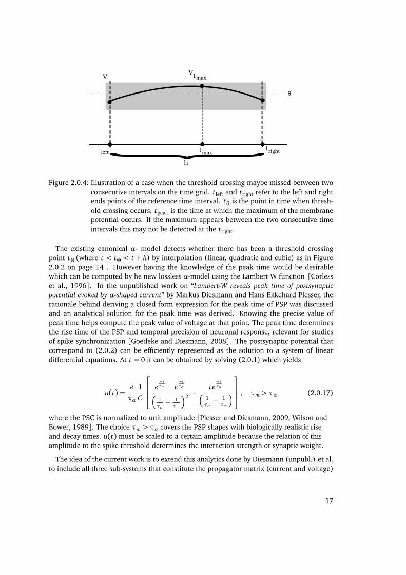
Figure 2.0.4: Illustration of a case when the threshold crossing maybe missed between twoconsecutive intervals on the time grid. tleft and tright refer to the left and rightends points of the reference time interval. tθ is the point in time when thresh-old crossing occurs, tpeak is the time at which the maximum of the membranepotential occurs. If the maximum appears between the two consecutive timeintervals this may not be detected at the tright.
The existing canonical α- model detects whether there has been a threshold crossingpoint tΘ (where t < tΘ < t + h) by interpolation (linear, quadratic and cubic) as in Figure2.0.2 on page 14 . However having the knowledge of the peak time would be desirablewhich can be computed by he new lossless α-model using the Lambert W function [Corlesset al., 1996]. In the unpublished work on “Lambert-W reveals peak time of postsynapticpotential evoked by α-shaped current” by Markus Diesmann and Hans Ekkehard Plesser, therationale behind deriving a closed form expression for the peak time of PSP was discussedand an analytical solution for the peak time was derived. Knowing the precise value ofpeak time helps compute the peak value of voltage at that point. The peak time determinesthe rise time of the PSP and temporal precision of neuronal response, relevant for studiesof spike synchronization [Goedeke and Diesmann, 2008]. The postsynaptic potential thatcorrespond to (2.0.2) can be efficiently represented as the solution to a system of lineardifferential equations. At t = 0 it can be obtained by solving (2.0.1) which yields
u(t) =e
τα
1
C
e−tτm − e
−tτα
�
1τα− 1τm
�2 −te−tτα
�
1τα− 1τm
�
, τm > τα (2.0.17)
where the PSC is normalized to unit amplitude [Plesser and Diesmann, 2009, Wilson andBower, 1989]. The choice τm > τα covers the PSP shapes with biologically realistic riseand decay times. u(t) must be scaled to a certain amplitude because the relation of thisamplitude to the spike threshold determines the interaction strength or synaptic weight.
The idea of the current work is to extend this analytics done by Diesmann (unpubl.) et al.to include all three sub-systems that constitute the propagator matrix (current and voltage)
17

2 Subthreshold dynamics in time-driven simulations
(2.0.8) and get an explicit expression for the peak time of PSP using the Lambert W function[Corless et al., 1996]. This result can then be used to construct tests to be included in thecanonical α-model of the precise spike timing framework to catch the spike misses thathappen between grid points.
18
3 Determination of peak time using Lambert Wfunction
The peak time of PSP refers to the point in time where the voltage reaches its maximum.InChapter 2 it was motivated that knowledge of the exact location of peak in the temporalspace reduces artificial synchronization and integration error. The time to maximum canthen be computed using the Lambert W function [Corless et al., 1996] as enumerated in thefollowing sections of this chapter.
3.1 Lambert W function
The Lambert W function defined by W (x) is the inverse of the function f (x) = xex ,satisfying
W (x)eW (x) = x (3.1.1)
for any complex number x , and W is any complex number. Since the function is notinjective, the relation W is multivalued except at zero [Corless et al., 1996].
19
3 Determination of peak time using Lambert W function
A
B
x W (x)x > 0 unique real rootsx = 0 0
−1e< x < 0 negative real roots :W0(x), W−1(x)
x = −1e
−1x < −1
eno real solutions
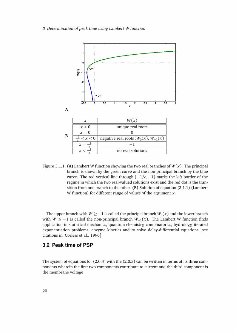
Figure 3.1.1: (A) Lambert W function showing the two real branches of W (x). The principalbranch is shown by the green curve and the non-principal branch by the bluecurve. The red vertical line through (−1/e,−1) marks the left border of theregime in which the two real-valued solutions exist and the red dot is the tran-sition from one branch to the other. (B) Solution of equation (3.1.1) (LambertW function) for different range of values of the argument x .
The upper branch with W ≥−1 is called the principal branch W0(x) and the lower branchwith W ≤ −1 is called the non-principal branch W−1(x). The Lambert W function findsapplication in statistical mechanics, quantum chemistry, combinatorics, hydrology, iteratedexponentiation problems, enzyme kinetics and to solve delay-differential equations [seecitations in Corless et al., 1996].
3.2 Peak time of PSP
The system of equations for (2.0.4) with the (2.0.5) can be written in terms of its three com-ponents wherein the first two components contribute to current and the third component isthe membrane voltage
20

3.2 Peak time of PSP
y1 = −1
ταy1+ i
e
τα(3.2.1)
y2 = −1
ταy2+ y1 (3.2.2)
y3 =1
Cy2−
1
τmy3. (3.2.3)
The derivative of (2.0.17) is
u(t) =e
τα
1
c
−1τα
e−tτm + 1
ταe−tτα
�
1τα− 1τm
�2 −e−tτα − 1
ταte−tτα
�
1τα− 1τm
�
(3.2.4)
The homogeneous solution y2 is
yh2 = e−
tτα (3.2.5)
and the particular solution that vanishes at t = 0 is
y2(t) = yh2
ˆ t
0(yh
2(t′))−1 y(t ′) d t ′
= e−tτα
ˆ t
0e
t′τα y1(0)e
− t′τα d t ′
=⇒ y2(t) = y1(0)te−tτα . (3.2.6)
We can determine the maximum of the α-function from y2 = 0
y1(0)�−1
τα
�
te−tτα + y1(0)e
−tτα = 0
=⇒ y1(0)
−t
τα+ 1
︸ ︷︷ ︸
(t=τα)⇒0
e−tτα = 0 (3.2.7)
From (3.2.6) and (3.2.7)
y2(τα) = y1(0)ταe−1 (3.2.8)
From (2.0.5) and (2.0.10) we have the initial relation for computation of peak time of PSPgiven by 0= y3 =
1C
y2−1τm
y3
21

3 Determination of peak time using Lambert W function
0=1
C
h
y2(0)e−tτα + y1(0)te
−tτα
i
−1
τm
y1(0)1
C
e−tτm − e
−tτα
�
1τα− 1τm
�2 −te−tτα
�
1τα− 1τm
�
+ y2(0)1
C
�
e−tτm − e
−tτα
�
�
1τα− 1τm
� + y3(0)e−tτm
(3.2.9)
Re-arranging the expression,
0 = y1(0)
te−tτα
1+
1
τm�
1τα− 1τm
�
−
1
τm
e−tτm − e
−tτα
�
1τα− 1τm
�2
+ y2(0)
e−tτα −
1
τm
�
e−tτm − e
−tτα
�
�
1τα− 1τm
�
−
C
τmy3(0)e
−tτm
0 = y1(0)
τm
τm −ταte−tτα −
1
τm
�
e−tτm − e
−tτα
�
�
1τα− 1τm
�2
+ y2(0)
e−tτα −
�
e−tτm − e
−tτα
�
τm�
1τm− 1τα
�
−
C
τmy3(0)e
−tτm (3.2.10)
we define
�
1
τα−
1
τm
�
= b andτm
τα= a, (3.2.11)
where a is the ratio of the two constants and must be greater than 1. With a and b werewrite the last expression as
0 = y1(0)
1�
1− 1a
� te−tτα −
1
τm
�
e−tτm − e
−tτα
�
b2
+ y2(0)
e−tτα −
�
e−tτm − e
−tτα
�
τm b
−C
τmy3(0)e
−tτm
and get,
e−tτm
�
y1(0)1
b2
1
τm+ y2(0)
1
τm b+
C
τmy3(0)
�
= e−tτα
y1(0)
1�
1− 1a
� t +1
τm b2
!
+ y2(0)�
1+1
τm b
�
e
�−1
τm+
1
τα
�
︸ ︷︷ ︸
b
t
=y1(0)
�
t
(1− 1a )+ 1τm b2
�
+ y2(0)�
1+ 1τm b
�
1τm b
�
y1(0)1b+ y2(0)
�
+ Cτm
y3(0). (3.2.12)
In order to solve for t we bring the expression to a form that can be solved by the LambertW function
ebt�
1
τm b
�
y1(0)1
b+ y2(0)
�
+C
τmy3(0)
�
−
y1(0)
t�
1− 1a
� +1
τm b2
!
+ y2(0)�
1+1
τm b
�
= 0
(3.2.13)or
22

3.2 Peak time of PSP
ebt −
y1(0)�
t�
1− 1a
� + 1τm b2
�
+ y2(0)�
1+ 1τm b
�
1τm b
�
y1(0)1b+ y2(0)
�
+ Cτm
y3(0)
= 0. (3.2.14)
We now define
s = bt, (3.2.15)
where s is scaled time and must be positive. (3.2.14) is of the form
es = a′s+ f (3.2.16)
Consider (3.2.11)
b�
1−1
a
�
=�
1
τα−
1
τm
��
1−τα
τm
�
=
�
τm−τα�2
τ2mτα
=
�
τm−τα�2
�
τmτα�2 τα
= ταb2. (3.2.17)
Writing (3.2.14) explicitly in terms of (3.2.16)
a′ =y1(0)
1ταb2
1τm b(y1(0)
1b+ y2(0)) +
Cτm
y3(0)(3.2.18)
f =y1(0)
1τm b2 + y2(0)
�
1+ 1τm b
�
1τm b
�
y1(0)1b+ y2(0)
�
+ Cτm
y3(0)(3.2.19)
Lambert W solves (3.1.1)
1 = ( f + a′s)e−s
−1
a=
�
−f
a′− s�
e−s
−1
a′e
fa′
︸ ︷︷ ︸
=
− f
a′− s
︸ ︷︷ ︸
w
e
− f
a′− s
︸ ︷︷ ︸
w
s = −W�−1
a′e− fa′
�
−f
a′. (3.2.20)
Plugging in (3.2.18) and (3.2.19) in (3.2.20) the peak time of PSP reads
23
3 Determination of peak time using Lambert W function
s =−W
−1τm b(y1(0)
1b+ y2(0)) +
Cτm
y3(0)
y1(0)1
ταb2
e−
y1(0)1
τm b2 +y2(0)�
1+ 1τm b
�
y1(0)1
τα b2
−y1(0)
1τm b2 + y2(0)
�
1+ 1τm b
�
y1(0)1
ταb2
.
(3.2.21)
Preliminary checks for validity and accuracy of this solution was done using Python[Python Software Foundation, 2008] and then implemented in NEST [Diesmann and Gewaltig,2002].
24
3.2 Peak time of PSP
A0 5 10 15 20 25 30 35 40 45 50 55 60 65 70 75 80 85 90 95
Time(ms)
0
5
10
15
20
Mem
bran
eVo
ltage
(mV
)
B5 10 15
Time(ms)
20
Mem
bran
eVo
ltage
(mV
)
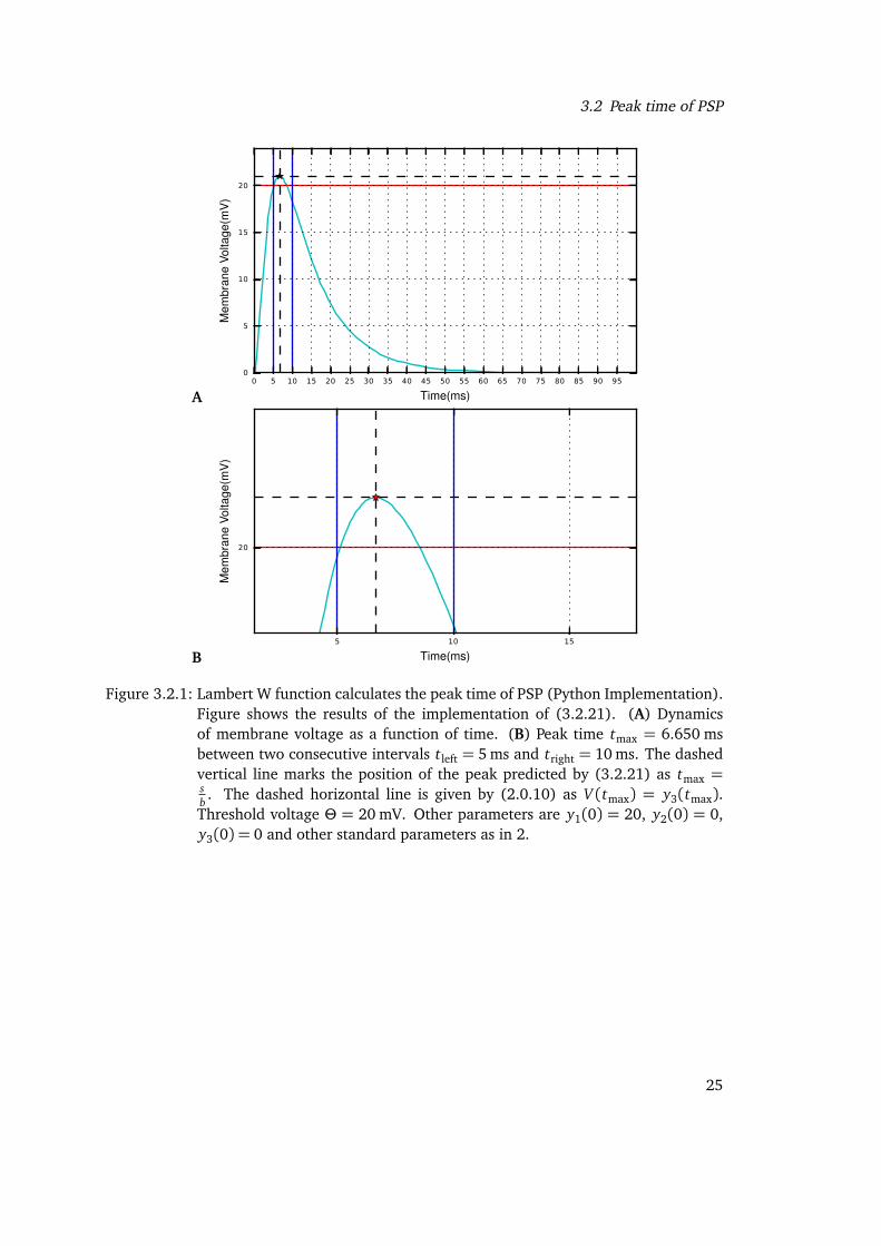
Figure 3.2.1: Lambert W function calculates the peak time of PSP (Python Implementation).Figure shows the results of the implementation of (3.2.21). (A) Dynamicsof membrane voltage as a function of time. (B) Peak time tmax = 6.650 msbetween two consecutive intervals tleft = 5 ms and tright = 10 ms. The dashedvertical line marks the position of the peak predicted by (3.2.21) as tmax =sb. The dashed horizontal line is given by (2.0.10) as V (tmax) = y3(tmax).
Threshold voltage Θ = 20 mV. Other parameters are y1(0) = 20, y2(0) = 0,y3(0) = 0 and other standard parameters as in 2.
25
3 Determination of peak time using Lambert W function
A0 20 40 60 80 100
Time(ms)
0
5
10
15
20
Mem
bran
eVo
ltage
(mV
)
B3 4 5 6 7 8 9 10
Time(ms)
13
14
15
16
17
18
19
20
Mem
bran
eVo
ltage
(mV
)
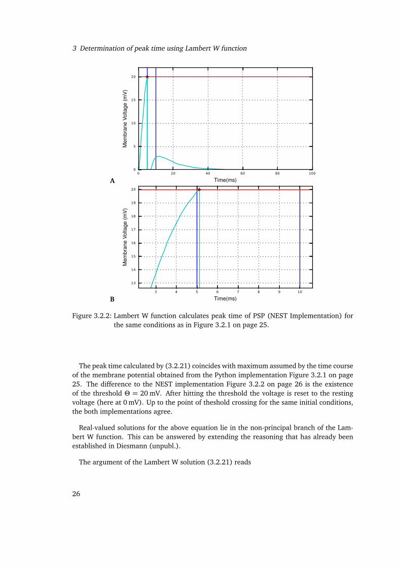
Figure 3.2.2: Lambert W function calculates peak time of PSP (NEST Implementation) forthe same conditions as in Figure 3.2.1 on page 25.
The peak time calculated by (3.2.21) coincides with maximum assumed by the time courseof the membrane potential obtained from the Python implementation Figure 3.2.1 on page25. The difference to the NEST implementation Figure 3.2.2 on page 26 is the existenceof the threshold Θ = 20 mV. After hitting the threshold the voltage is reset to the restingvoltage (here at 0 mV). Up to the point of theshold crossing for the same initial conditions,the both implementations agree.
Real-valued solutions for the above equation lie in the non-principal branch of the Lam-bert W function. This can be answered by extending the reasoning that has already beenestablished in Diesmann (unpubl.).
The argument of the Lambert W solution (3.2.21) reads
26

3.3 Critical conditions
arg(W ) = −1τm b(y1(0)
1b+ y2(0)) +
Cτm
y3(0)
y1(0)1
ταb2
e
−y1(0)
1τm b2 + y2(0)
�
1+ 1τm b
�
y1(0)1
ταb2︸ ︷︷ ︸
p (3.2.22)
=−1
a
1b
�
y1(0)1b+ y2(0)
�
+ C y3(0)
y1(0)1b2
ep.
From (3.2.11) and (3.2.21) we have
W <−1
a(3.2.23)
since s > 0 and a > 1 in the interval −1e< arg(W ) < 0. This interval is bounded by the line
e x Figure 3.1.1 on page 20 which leads to the condition that
−1
a<W< e x (3.2.24)
that means that there can be no solution for this equation in the principal branch.
3.3 Critical conditions
3.3.1 Initial condition y1(0) = 0
Looking at the solution (3.2.21) we see that for the case y1(0) = 0 there is no solution. Thismotivates the need for an expression for this special case. Starting from (3.2.12) we obtain
e
�−1
τm+
1
τα
�
︸ ︷︷ ︸
b
t
=y1(0)
�
t�
1− 1a
� + 1τm b2
�
+ y2(0)�
1+ 1τm b
�
1τm b
�
y1(0)1b+ y2(0)
�
+ Cτm
y3(0)
ebt =y2(0)
�
1+ 1τm b
�
1τm b
y2(0) +Cτm
y3(0)
s = log
y2(0)�
1+ 1τm b
�
1τm b
y2(0) +Cτm
y3(0)
t =1
blog
y2(0)�
1+ 1τm b
�
1τm b
y2(0) +Cτm
y3(0)
(3.3.1)
27
3 Determination of peak time using Lambert W function
A 0 5 10 15 20 25 30 35 40 45 50 55 60 65 70 75 80 85 90 950
5
10
15
20
Mem
bran
eVo
ltage
(mV
)
B0 5
Time(ms)
20
Mem
bran
eVo
ltage
(mV
)
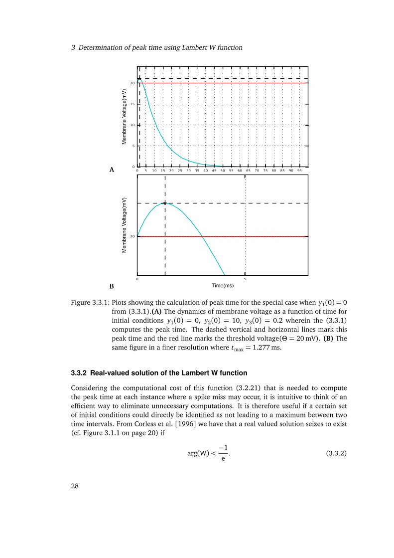
Figure 3.3.1: Plots showing the calculation of peak time for the special case when y1(0) = 0from (3.3.1).(A) The dynamics of membrane voltage as a function of time forinitial conditions y1(0) = 0, y2(0) = 10, y3(0) = 0.2 wherein the (3.3.1)computes the peak time. The dashed vertical and horizontal lines mark thispeak time and the red line marks the threshold voltage(Θ = 20 mV). (B) Thesame figure in a finer resolution where tmax = 1.277 ms.
3.3.2 Real-valued solution of the Lambert W function
Considering the computational cost of this function (3.2.21) that is needed to computethe peak time at each instance where a spike miss may occur, it is intuitive to think of anefficient way to eliminate unnecessary computations. It is therefore useful if a certain setof initial conditions could directly be identified as not leading to a maximum between twotime intervals. From Corless et al. [1996] we have that a real valued solution seizes to exist(cf. Figure 3.1.1 on page 20) if
arg(W)<−1
e. (3.3.2)
28
3.3 Critical conditions
The idea is to check what range of initial conditions of the membrane voltage y3 this condi-tion (3.3.2) corresponds to. From (3.2.22) and (3.3.2) we have
−1
e>−
1τm b(y1(0)
1b+ y2(0)) +
Cτm
y3(0)
y1(0)1
ταb2
e−
y1(0)1
τm b2 +y2(0)�
1+ 1τm b
�
y1(0)1
τα b2 (3.3.3)
Multiplying both sides of (3.3.2) by −1 and flipping the unequal sign yields after insertionof (3.2.22)
1
e>
1τm b(y1(0)
1b+ y2(0)) +
Cτm
y3(0)
y1(0)1
ταb2
e−
y1(0)1
τm b2 +y2(0)�
1+ 1τm b
�
y1(0)1
τα b2 (3.3.4)
Solving for y3(0) we have
y3(0)<1
C
a
b2 y1(0)e
y1(0)1
τm b2 +y2(0)�
1+ 1τm b
�
y1(0)1
τα b2−1
−1
b(y1(0)
1
b+ y2(0))
(3.3.5)
The exponent can be re-written as
y1(0)1
τm b2 + y2(0)�
1+ 1τm b
�
y1(0)1
ταb2
− 1 =y1(0)
1τm b2 + y2(0)
�
1+ 1τm b
�
− y1(0)1
ταb2
y1(0)1
ταb2
=y2(0)
�
1+ 1τm b
�
− y1(0)b
y1(0)1
ταb2
=y2(0)y1(0)
�
1+1
τm b
�
ταb2−ταb
= by2(0)y1(0)
�
ταb+1
a
�
−ταb
= by2(0)y1(0)
−ταb (3.3.6)
From (3.3.5) and (3.3.6) we get
y3(0)<1
C
�
a
b2 y1(0)e
�
b y2(0)y1(0)−ταb
�
−1
b(y1(0)
1
b+ y2(0))
�
(3.3.7)
29
3 Determination of peak time using Lambert W function
0 20 40 60 80 100
Time(ms)
0.0
0.2
0.4
0.6
0.8
1.0
Mem
bran
eVo
ltage
(mV
)
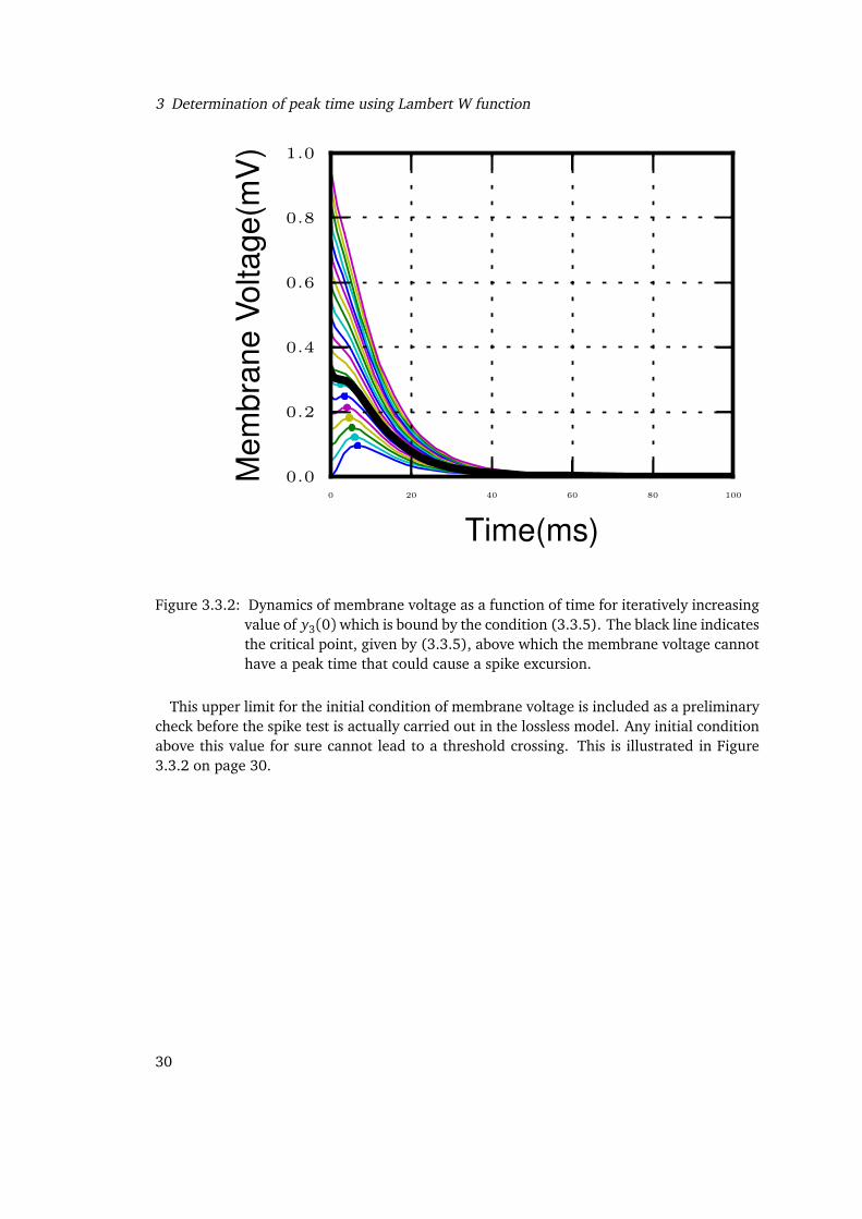
Figure 3.3.2: Dynamics of membrane voltage as a function of time for iteratively increasingvalue of y3(0)which is bound by the condition (3.3.5). The black line indicatesthe critical point, given by (3.3.5), above which the membrane voltage cannothave a peak time that could cause a spike excursion.
This upper limit for the initial condition of membrane voltage is included as a preliminarycheck before the spike test is actually carried out in the lossless model. Any initial conditionabove this value for sure cannot lead to a threshold crossing. This is illustrated in Figure3.3.2 on page 30.
30
4 Continuous-time spiking neuron models
4.1 NEST
The Neural Simulation Technology (NEST) initiative is a collaborative effort to develop anopen simulation framework for biologically realistic neuronal networks. A NEST simulationtries to mimic an electrophysiological experiment, which includes two conceptual domains:the description of the neuronal system and the description of the experimental setup andprotocol. NEST is written in object-oriented style (C++) [Diesmann and Gewaltig, 2002].The first user-interface to NEST [Gewaltig and Diesmann, 2007] was the simulation lan-guage SLI, a stack-based language derived from PostScript. A more conveniently usableinterface to NEST is the PyNEST, the Python interface to NEST. NEST defines the neuralworld in terms of directed, weighted graph of nodes and connections. Nodes are neurons,connections are characterized by a configurable fixed delay, and a weight that can be staticor dynamic. Several models for nodes and connections are built into NEST. Their parametersare accessed via dictionaries [Eppler et al., 2009].
4.2 α− neuron model
In the previous chapter Chapter 2 an outline of the canonical neuron model has been dis-cussed. The idea of combining exact integration of sub-threshold membrane dynamics withinterpolation to calculate the precise spike timing has been motivated in Chapter 2 usingillustrations Figure 2.0.2 on page 14 and Figure 2.0.3 on page 15. This chapter discussesan overview of the general algorithmic structure of the alpha models: canonical andlossless.
The key function that handles spike events in the alpha model is the update function.The update and spike handling function applies the time evolution operator and calls theemit_spike, propagate function and other auxiliary functions that processes events inthe time grid. The update function moves the state of the neuron from t0 to t0+ d t eitherin steps of resolution h, if there are no incoming spike events in the time interval or fromevent to event, as retrieved from the spike queue. The dynamics from one point to the otheris calculated using the propagator matrix. For steps in which there are no incoming spikeevents, it is handled by the fixed pre-computed propagator matrix.
31
4 Continuous-time spiking neuron models
} }+
θ
tleft
tright
lefttpeak
tpeakt
VtpeakV
point of reference(emit_spike) point of reference(spike_test)
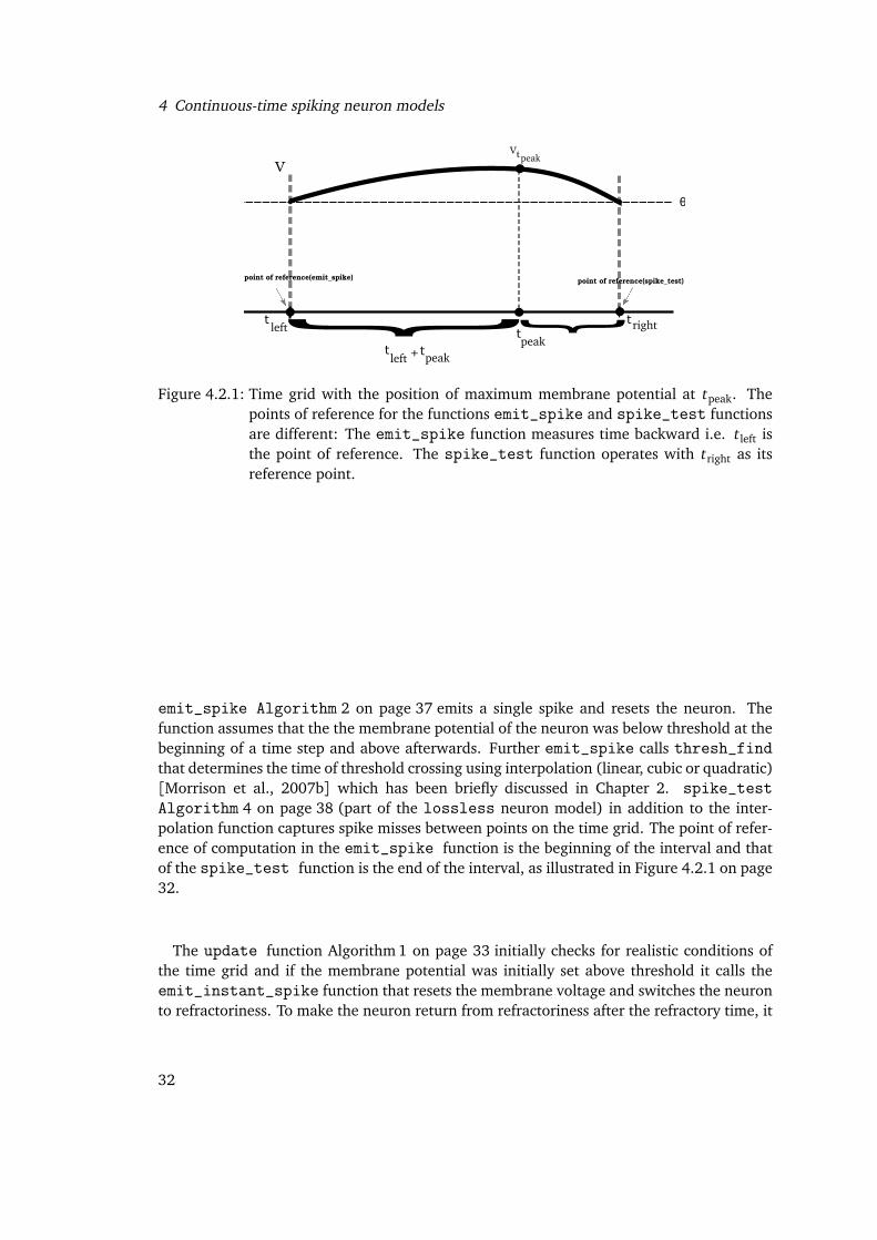
Figure 4.2.1: Time grid with the position of maximum membrane potential at tpeak. Thepoints of reference for the functions emit_spike and spike_test functionsare different: The emit_spike function measures time backward i.e. tleft isthe point of reference. The spike_test function operates with tright as itsreference point.
emit_spike Algorithm 2 on page 37 emits a single spike and resets the neuron. Thefunction assumes that the the membrane potential of the neuron was below threshold at thebeginning of a time step and above afterwards. Further emit_spike calls thresh_findthat determines the time of threshold crossing using interpolation (linear, cubic or quadratic)[Morrison et al., 2007b] which has been briefly discussed in Chapter 2. spike_testAlgorithm 4 on page 38 (part of the lossless neuron model) in addition to the inter-polation function captures spike misses between points on the time grid. The point of refer-ence of computation in the emit_spike function is the beginning of the interval and thatof the spike_test function is the end of the interval, as illustrated in Figure 4.2.1 on page32.
The update function Algorithm 1 on page 33 initially checks for realistic conditions ofthe time grid and if the membrane potential was initially set above threshold it calls theemit_instant_spike function that resets the membrane voltage and switches the neuronto refractoriness. To make the neuron return from refractoriness after the refractory time, it
32
4.2 α− neuron model
places a pseudoevent into the ring buffer, that, when processed, ends the refractory period.
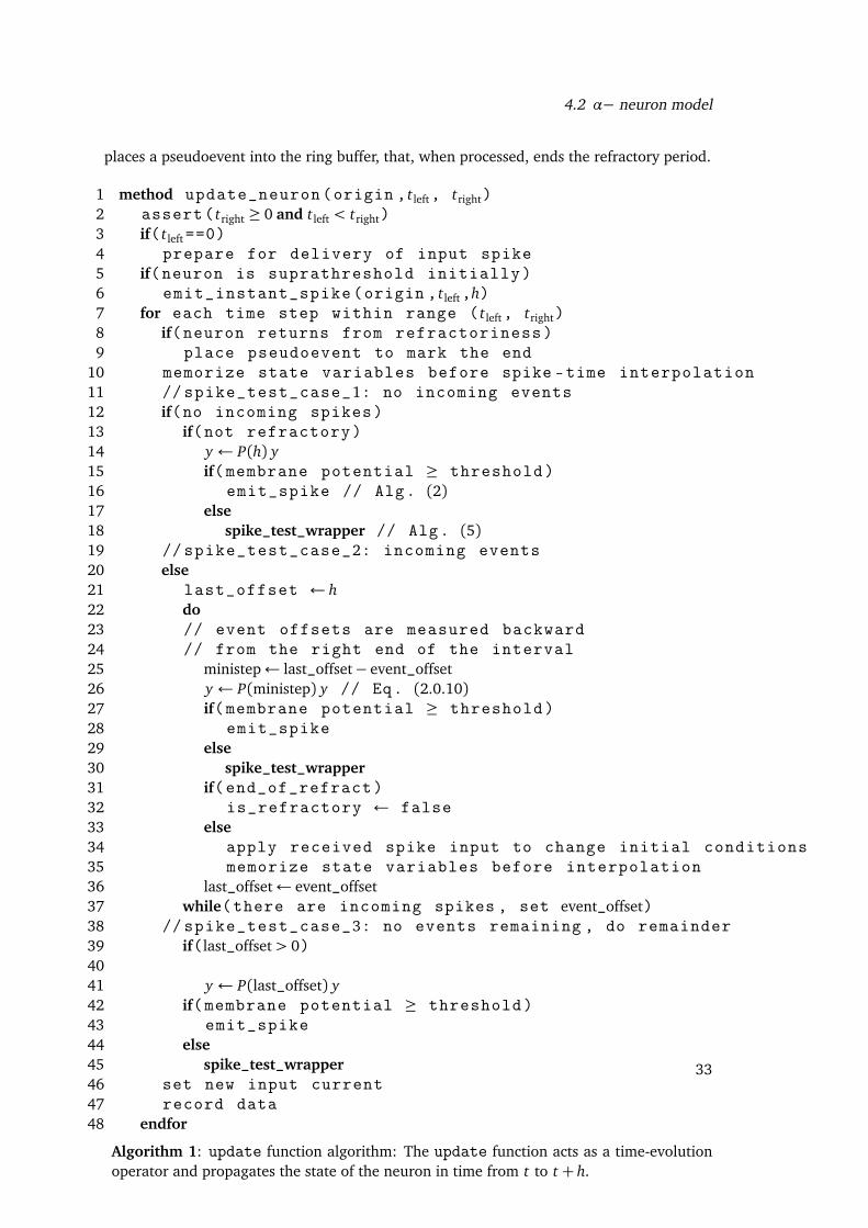
1 method update_neuron(origin , tleft, tright)2 assert( tright ≥ 0 and tleft < tright)3 if( tleft==0)4 prepare for delivery of input spike5 if(neuron is suprathreshold initially)6 emit_instant_spike(origin , tleft,h)7 for each time step within range ( tleft, tright)8 if(neuron returns from refractoriness)9 place pseudoevent to mark the end
10 memorize state variables before spike -time interpolation11 // spike_test_case_1: no incoming events12 if(no incoming spikes)13 if(not refractory)14 y ← P(h) y15 if(membrane potential ≥ threshold)16 emit_spike // Alg. (2)17 else18 spike_test_wrapper // Alg. (5)19 // spike_test_case_2: incoming events20 else21 last_offset ← h22 do23 // event offsets are measured backward24 // from the right end of the interval25 ministep← last_offset− event_offset26 y ← P(ministep) y // Eq. (2.0.10)27 if(membrane potential ≥ threshold)28 emit_spike29 else30 spike_test_wrapper31 if(end_of_refract)32 is_refractory ← false33 else34 apply received spike input to change initial conditions35 memorize state variables before interpolation36 last_offset← event_offset37 while(there are incoming spikes , set event_offset)38 // spike_test_case_3: no events remaining , do remainder39 if(last_offset> 0)4041 y ← P(last_offset) y42 if(membrane potential ≥ threshold)43 emit_spike44 else45 spike_test_wrapper46 set new input current47 record data48 endfor
Algorithm 1: update function algorithm: The update function acts as a time-evolutionoperator and propagates the state of the neuron in time from t to t + h.
33
4 Continuous-time spiking neuron models
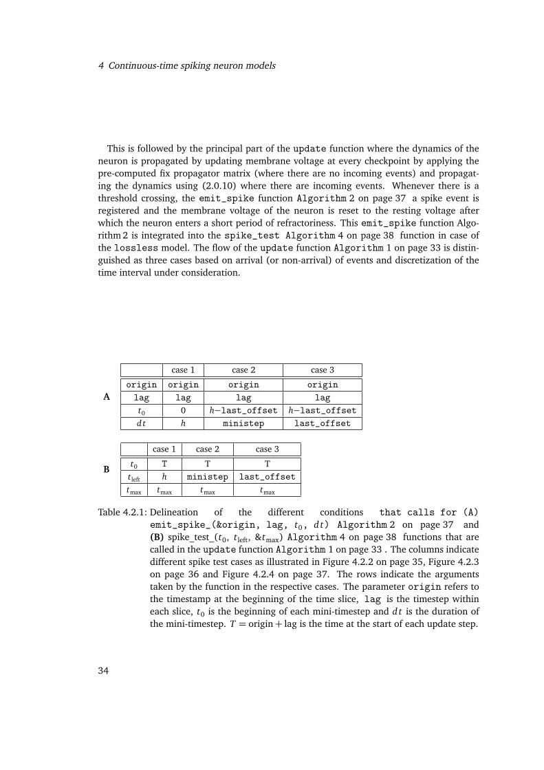
This is followed by the principal part of the update function where the dynamics of theneuron is propagated by updating membrane voltage at every checkpoint by applying thepre-computed fix propagator matrix (where there are no incoming events) and propagat-ing the dynamics using (2.0.10) where there are incoming events. Whenever there is athreshold crossing, the emit_spike function Algorithm 2 on page 37 a spike event isregistered and the membrane voltage of the neuron is reset to the resting voltage afterwhich the neuron enters a short period of refractoriness. This emit_spike function Algo-rithm 2 is integrated into the spike_test Algorithm 4 on page 38 function in case ofthe lossless model. The flow of the update function Algorithm 1 on page 33 is distin-guished as three cases based on arrival (or non-arrival) of events and discretization of thetime interval under consideration.
A
case 1 case 2 case 3
origin origin origin originlag lag lag lagt0 0 h−last_offset h−last_offsetd t h ministep last_offset
B
case 1 case 2 case 3
t0 T T Ttleft h ministep last_offsettmax tmax tmax tmax
Table 4.2.1: Delineation of the different conditions that calls for (A)emit_spike_(&origin, lag, t0, d t) Algorithm 2 on page 37 and(B) spike_test_(t0, tleft, &tmax) Algorithm 4 on page 38 functions that arecalled in the update function Algorithm 1 on page 33 . The columns indicatedifferent spike test cases as illustrated in Figure 4.2.2 on page 35, Figure 4.2.3on page 36 and Figure 4.2.4 on page 37. The rows indicate the argumentstaken by the function in the respective cases. The parameter origin refers tothe timestamp at the beginning of the time slice, lag is the timestep withineach slice, t0 is the beginning of each mini-timestep and d t is the duration ofthe mini-timestep. T = origin+ lag is the time at the start of each update step.
34
4.2 α− neuron model
θ
tleft
tright
Vtmax
V
maxt}h
no incoming event
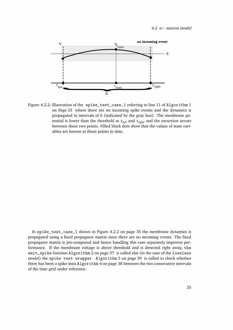
Figure 4.2.2: Illustration of the spike_test_case_1 referring to line 11 of Algorithm 1on Page 33 where there are no incoming spike events and the dynamics ispropagated in intervals of h (indicated by the gray box). The membrane po-tential is lower than the threshold at tleft and tright and the excursion occursbetween these two points. Filled black dots show that the values of state vari-ables are known at those points in time.
In spike_test_case_1 shown in Figure 4.2.2 on page 35 the membrane dynamics ispropagated using a fixed propagator matrix since there are no incoming events. The fixedpropagator matrix is pre-computed and hence handling this case separately improves per-formance. If the membrane voltage is above threshold and is detected right away, theemit_spike function Algorithm 2 on page 37 is called else (in the case of the losslessmodel) the spike test wrapper Algorithm 5 on page 39 is called to check whetherthere has been a spike miss Algorithm 4 on page 38 between the two consecutive intervalsof the time grid under reference.
35
4 Continuous-time spiking neuron models
θ
tleft tright
V tmaxV
maxt
there are incoming event(s)
last_offset = h last_offset = 0
event_offset
tθ
}ministep
𝛿 𝛿1 i
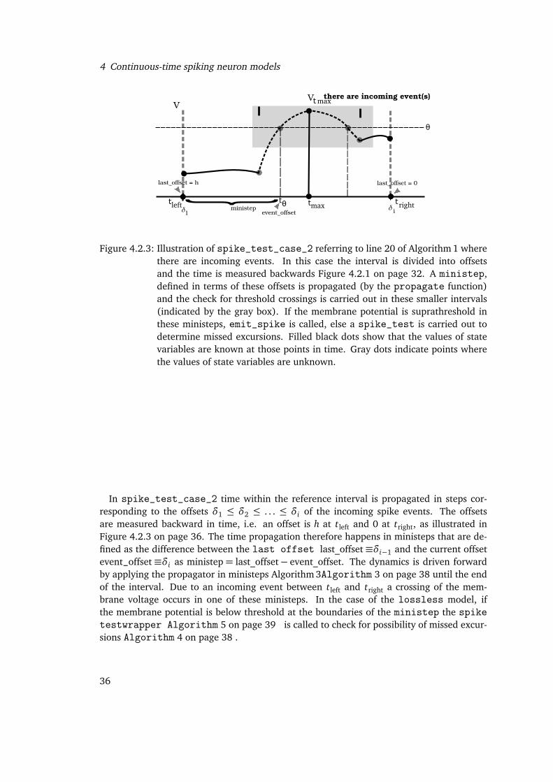
Figure 4.2.3: Illustration of spike_test_case_2 referring to line 20 of Algorithm 1 wherethere are incoming events. In this case the interval is divided into offsetsand the time is measured backwards Figure 4.2.1 on page 32. A ministep,defined in terms of these offsets is propagated (by the propagate function)and the check for threshold crossings is carried out in these smaller intervals(indicated by the gray box). If the membrane potential is suprathreshold inthese ministeps, emit_spike is called, else a spike_test is carried out todetermine missed excursions. Filled black dots show that the values of statevariables are known at those points in time. Gray dots indicate points wherethe values of state variables are unknown.
In spike_test_case_2 time within the reference interval is propagated in steps cor-responding to the offsets δ1 ≤ δ2 ≤ . . . ≤ δi of the incoming spike events. The offsetsare measured backward in time, i.e. an offset is h at tleft and 0 at tright, as illustrated inFigure 4.2.3 on page 36. The time propagation therefore happens in ministeps that are de-fined as the difference between the last offset last_offset≡δi−1 and the current offsetevent_offset≡δi as ministep= last_offset− event_offset. The dynamics is driven forwardby applying the propagator in ministeps Algorithm 3Algorithm 3 on page 38 until the endof the interval. Due to an incoming event between tleft and tright a crossing of the mem-brane voltage occurs in one of these ministeps. In the case of the lossless model, ifthe membrane potential is below threshold at the boundaries of the ministep the spiketestwrapper Algorithm 5 on page 39 is called to check for possibility of missed excur-sions Algorithm 4 on page 38 .
36
4.2 α− neuron model
θ
tleft
tright
Vtmax
V
maxt
no incoming event: plain update of the remainder step
𝛿i-1}last_offset > 0
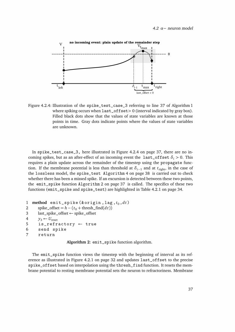
Figure 4.2.4: Illustration of the spike_test_case_3 referring to line 37 of Algorithm 1where spiking occurs when last_offset> 0 (interval indicated by gray box).Filled black dots show that the values of state variables are known at thosepoints in time. Gray dots indicate points where the values of state variablesare unknown.
In spike_test_case_3, here illustrated in Figure 4.2.4 on page 37, there are no in-coming spikes, but as an after-effect of an incoming event the last_offset δi > 0. Thisrequires a plain update across the remainder of the timestep using the propagate func-tion. If the membrane potential is less than threshold at δi−1 and at tright, in the case ofthe lossless model, the spike_test Algorithm 4 on page 38 is carried out to checkwhether there has been a missed spike. If an excursion is detected between these two points,the emit_spike function Algorithm 2 on page 37 is called. The specifics of these twofunctions (emit_spike and spike_test) are highlighted in Table 4.2.1 on page 34.
1 method emit_spike (&origin ,lag , t0,d t)2 spike_offset= h− (t0+ thresh_find(d t))3 last_spike_offset← spike_offset4 y3← Ureset5 is_refractory ← true6 send spike7 return
Algorithm 2: emit_spike function algorithm.
The emit_spike function views the timestep with the beginning of interval as its ref-erence as illustrated in Figure 4.2.1 on page 32 and updates last_offset to the precisespike_offset based on interpolation using the thresh_find function. It resets the mem-brane potential to resting membrane potential sets the neuron to refractoriness. Membrane
37
4 Continuous-time spiking neuron models
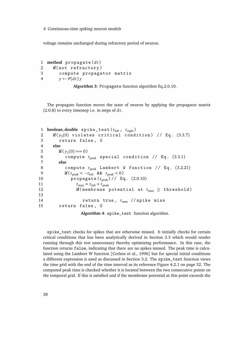
voltage remains unchanged during refractory period of neuron.
1 method propagate(d t)2 if(not refractory)3 compute propagator matrix4 y ← P(d t) y
Algorithm 3: Propagate function algorithm Eq.2.0.10.
The propagate function moves the state of neuron by applying the propagator matrix(2.0.8) to every timestep i.e. in steps of d t.
1 boolean,double spike_test( tleft, tright)2 if( y3(0) violates critical condition) // Eq. (3.3.7)3 return false , 04 else5 if( y1(0) == 0)6 compute tpeak special condition // Eq. (3.3.1)7 else8 compute tpeak Lambert W function // Eq. (3.2.21)9 if( tpeak <−tleft && tpeak < 0)
10 propagate( tpeak)// Eq. (2.0.10)11 tmax = tleft+ tpeak12 if(membrane potential at tmax ≥ threshold)1314 return true , tmax //spike miss15 return false , 0
Algorithm 4: spike_test function algorithm.
spike_test checks for spikes that are otherwise missed. It initially checks for certaincritical conditions that has been analytically derived in Section 3.3 which would renderrunning through this test unnecessary thereby optimizing performance. In this case, thefunction returns false, indicating that there are no spikes missed. The peak time is calcu-lated using the Lambert W function [Corless et al., 1996] but for special initial conditionsa different expression is used as discussed in Section 3.2. The spike_test function viewsthe time grid with the end of the time interval as its reference Figure 4.2.1 on page 32. Thecomputed peak time is checked whether it is located between the two consecutive points onthe temporal grid. If this is satisfied and if the membrane potential at this point exceeds the
38
4.3 Spike test
threshold, then a spike has been certainly missed, and the function returns true.
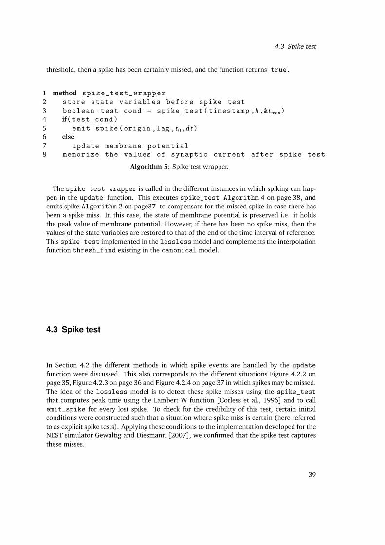
1 method spike_test_wrapper2 store state variables before spike test3 boolean test_cond = spike_test(timestamp ,h,& tmax)4 if(test_cond)5 emit_spike(origin ,lag , t0,d t)6 else7 update membrane potential8 memorize the values of synaptic current after spike test
Algorithm 5: Spike test wrapper.
The spike test wrapper is called in the different instances in which spiking can hap-pen in the update function. This executes spike_test Algorithm 4 on page 38, andemits spike Algorithm 2 on page37 to compensate for the missed spike in case there hasbeen a spike miss. In this case, the state of membrane potential is preserved i.e. it holdsthe peak value of membrane potential. However, if there has been no spike miss, then thevalues of the state variables are restored to that of the end of the time interval of reference.This spike_test implemented in the lossless model and complements the interpolationfunction thresh_find existing in the canonical model.
4.3 Spike test
In Section 4.2 the different methods in which spike events are handled by the updatefunction were discussed. This also corresponds to the different situations Figure 4.2.2 onpage 35, Figure 4.2.3 on page 36 and Figure 4.2.4 on page 37 in which spikes may be missed.The idea of the lossless model is to detect these spike misses using the spike_testthat computes peak time using the Lambert W function [Corless et al., 1996] and to callemit_spike for every lost spike. To check for the credibility of this test, certain initialconditions were constructed such that a situation where spike miss is certain (here referredto as explicit spike tests). Applying these conditions to the implementation developed for theNEST simulator Gewaltig and Diesmann [2007], we confirmed that the spike test capturesthese misses.
39
4 Continuous-time spiking neuron models
A
0 20 40 60 80 100
Time(ms)
0
5
10
15
20
Mem
bran
eVo
ltage
(mV
)
h=0.01h=5.0
B
4 5 6 7 8 9 10 11
Time(ms)
19.0
19.2
19.4
19.6
19.8
20.0
20.2
20.4
Mem
bran
eVo
ltage
(mV
)
h=0.01h=5.0
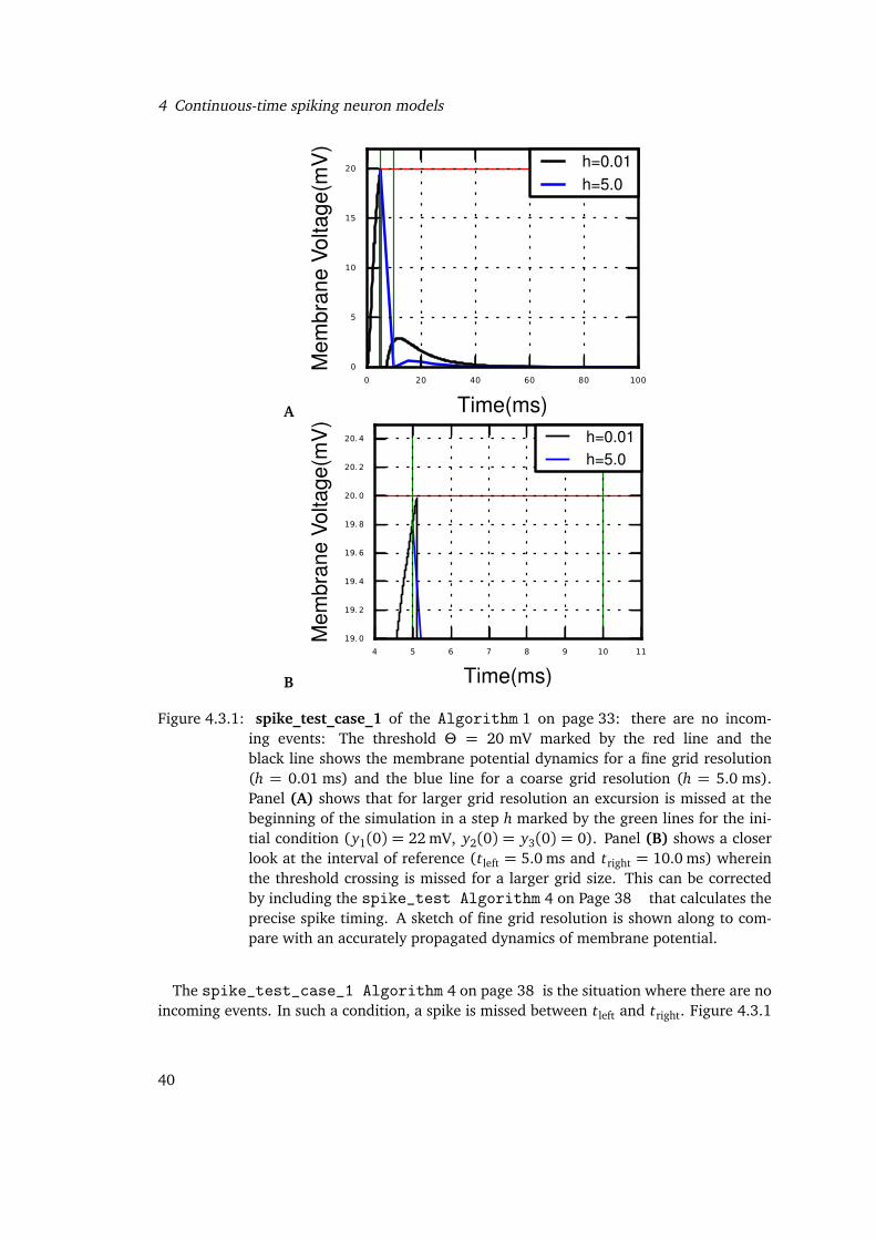
Figure 4.3.1: spike_test_case_1 of the Algorithm 1 on page 33: there are no incom-ing events: The threshold Θ = 20 mV marked by the red line and theblack line shows the membrane potential dynamics for a fine grid resolution(h = 0.01 ms) and the blue line for a coarse grid resolution (h = 5.0 ms).Panel (A) shows that for larger grid resolution an excursion is missed at thebeginning of the simulation in a step h marked by the green lines for the ini-tial condition (y1(0) = 22 mV, y2(0) = y3(0) = 0). Panel (B) shows a closerlook at the interval of reference (tleft = 5.0 ms and tright = 10.0 ms) whereinthe threshold crossing is missed for a larger grid size. This can be correctedby including the spike_test Algorithm 4 on Page 38 that calculates theprecise spike timing. A sketch of fine grid resolution is shown along to com-pare with an accurately propagated dynamics of membrane potential.
The spike_test_case_1 Algorithm 4 on page 38 is the situation where there are noincoming events. In such a condition, a spike is missed between tleft and tright. Figure 4.3.1
40
4.3 Spike test
on page 40 shows that for large grid resolution such excursions are missed but can be caughtby the spike_test Algorithm 4 on page 38 .
A
0 20 40 60 80 100
Time(ms)
0
5
10
15
20
Mem
bran
eVo
ltage
(mV
)
h=0.01h=5.0
B4.0 4.5 5.0 5.5 6.0 6.5 7.0 7.5 8.0
Time(ms)
18.0
18.5
19.0
19.5
20.0
20.5
Mem
bran
eVo
ltage
(mV
)
h=0.01h=5.0
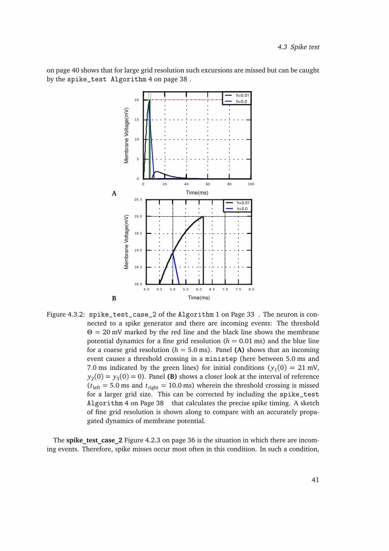
Figure 4.3.2: spike_test_case_2 of the Algorithm 1 on Page 33 . The neuron is con-nected to a spike generator and there are incoming events: The thresholdΘ = 20 mV marked by the red line and the black line shows the membranepotential dynamics for a fine grid resolution (h = 0.01 ms) and the blue linefor a coarse grid resolution (h = 5.0 ms). Panel (A) shows that an incomingevent causes a threshold crossing in a ministep (here between 5.0 ms and7.0 ms indicated by the green lines) for initial conditions (y1(0) = 21 mV,y2(0) = y3(0) = 0). Panel (B) shows a closer look at the interval of reference(tleft = 5.0 ms and tright = 10.0 ms) wherein the threshold crossing is missedfor a larger grid size. This can be corrected by including the spike_testAlgorithm 4 on Page 38 that calculates the precise spike timing. A sketchof fine grid resolution is shown along to compare with an accurately propa-gated dynamics of membrane potential.
The spike_test_case_2 Figure 4.2.3 on page 36 is the situation in which there are incom-ing events. Therefore, spike misses occur most often in this condition. In such a condition,
41
4 Continuous-time spiking neuron models
a spike is missed in a ministep. Figure 4.3.2 on page 41 shows that for large grid resolu-tion such excursions are missed but can be caught by the spike_test Algorithm 4 onpage 38 .
A0 20 40 60 80 100
Time(ms)
0
5
10
15
20
Mem
bran
eVo
ltage
(mV
)
h=0.01h=5.0
B10 12 14 16 18 20
Time(ms)
18.0
18.5
19.0
19.5
20.0
20.5
Mem
bran
eVo
ltage
(mV
)
h=0.01h=5.0
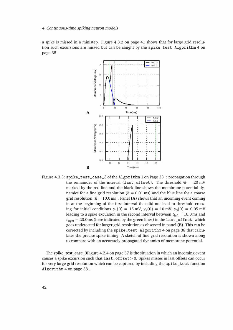
Figure 4.3.3: spike_test_case_3 of the Algorithm 1 on Page 33 : propagation throughthe remainder of the interval (last_offset): The threshold Θ = 20 mVmarked by the red line and the black line shows the membrane potential dy-namics for a fine grid resolution (h = 0.01 ms) and the blue line for a coarsegrid resolution (h= 10.0ms). Panel (A) shows that an incoming event comingin at the beginning of the first interval that did not lead to threshold cross-ing for initial conditions y1(0) = 15 mV, y2(0) = 10 mV, y3(0) = 0.05 mVleading to a spike excursion in the second interval between tleft = 10.0ms andtright = 20.0ms (here indicated by the green lines) in the last_offset whichgoes undetected for larger grid resolution as observed in panel (B). This can becorrected by including the spike_test Algorithm 4 on page 38 that calcu-lates the precise spike timing. A sketch of fine grid resolution is shown alongto compare with an accurately propagated dynamics of membrane potential.
The spike_test_case_3Figure 4.2.4 on page 37 is the situation in which an incoming eventcauses a spike excursion such that last_offset> 0. Spikes misses in last offsets can occurfor very large grid resolution which can be captured by including the spike_test functionAlgorithm 4 on page 38 .
42
4.4 Neuron embedded in a quasi-network setup
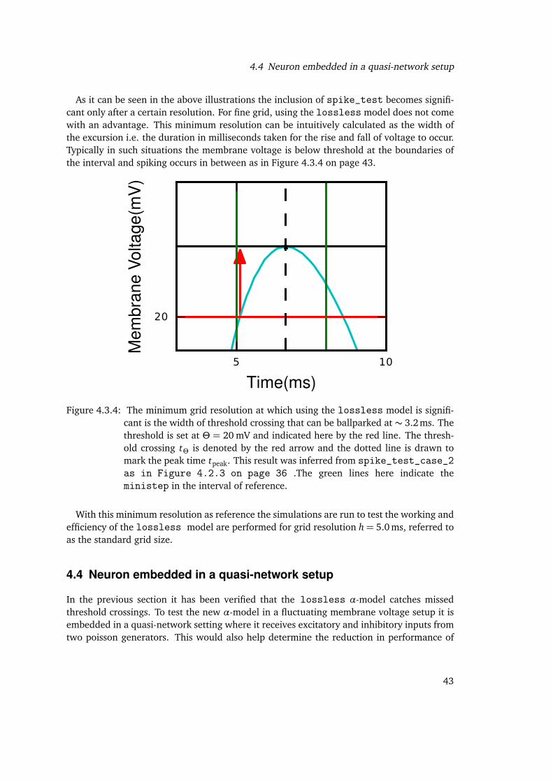
As it can be seen in the above illustrations the inclusion of spike_test becomes signifi-cant only after a certain resolution. For fine grid, using the lossless model does not comewith an advantage. This minimum resolution can be intuitively calculated as the width ofthe excursion i.e. the duration in milliseconds taken for the rise and fall of voltage to occur.Typically in such situations the membrane voltage is below threshold at the boundaries ofthe interval and spiking occurs in between as in Figure 4.3.4 on page 43.
5 10
Time(ms)
20
Mem
bran
eVo
ltage
(mV
)
Figure 4.3.4: The minimum grid resolution at which using the lossless model is signifi-cant is the width of threshold crossing that can be ballparked at ∼ 3.2ms. Thethreshold is set at Θ = 20 mV and indicated here by the red line. The thresh-old crossing tΘ is denoted by the red arrow and the dotted line is drawn tomark the peak time tpeak. This result was inferred from spike_test_case_2as in Figure 4.2.3 on page 36 .The green lines here indicate theministep in the interval of reference.
With this minimum resolution as reference the simulations are run to test the working andefficiency of the lossless model are performed for grid resolution h= 5.0 ms, referred toas the standard grid size.
4.4 Neuron embedded in a quasi-network setup
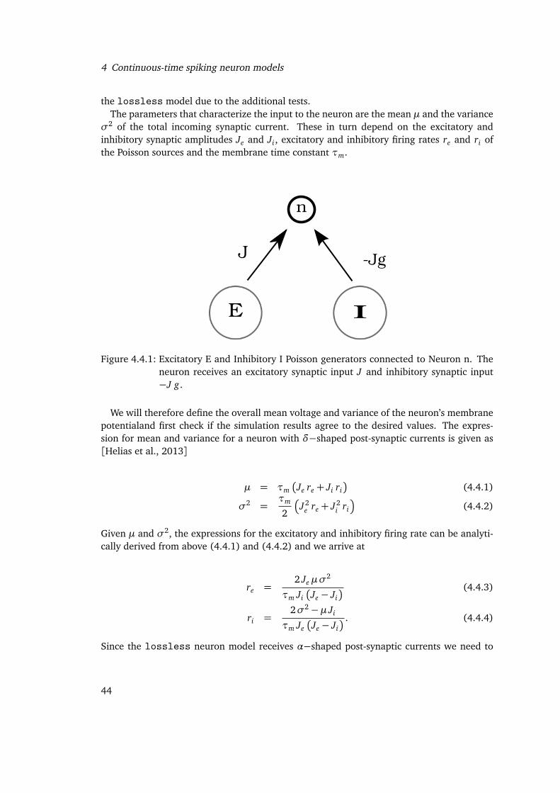
In the previous section it has been verified that the lossless α-model catches missedthreshold crossings. To test the new α-model in a fluctuating membrane voltage setup it isembedded in a quasi-network setting where it receives excitatory and inhibitory inputs fromtwo poisson generators. This would also help determine the reduction in performance of
43
4 Continuous-time spiking neuron models
the lossless model due to the additional tests.The parameters that characterize the input to the neuron are the mean µ and the variance
σ2 of the total incoming synaptic current. These in turn depend on the excitatory andinhibitory synaptic amplitudes Je and Ji , excitatory and inhibitory firing rates re and ri ofthe Poisson sources and the membrane time constant τm.
E I
n
J -Jg
Figure 4.4.1: Excitatory E and Inhibitory I Poisson generators connected to Neuron n. Theneuron receives an excitatory synaptic input J and inhibitory synaptic input−J g.
We will therefore define the overall mean voltage and variance of the neuron’s membranepotentialand first check if the simulation results agree to the desired values. The expres-sion for mean and variance for a neuron with δ−shaped post-synaptic currents is given as[Helias et al., 2013]
µ = τm�
Je re + Ji ri�
(4.4.1)
σ2 =τm
2
�
J2e re + J2
i ri
�
(4.4.2)
Given µ and σ2, the expressions for the excitatory and inhibitory firing rate can be analyti-cally derived from above (4.4.1) and (4.4.2) and we arrive at
re =2 Je µσ
2
τm Ji�
Je − Ji� (4.4.3)
ri =2σ2−µ Ji
τm Je�
Je − Ji� . (4.4.4)
Since the lossless neuron model receives α−shaped post-synaptic currents we need to
44
4.4 Neuron embedded in a quasi-network setup
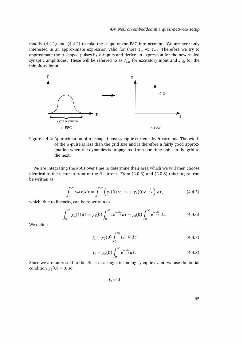
modify (4.4.1) and (4.4.2) to take the shape of the PSC into account. We are here onlyinterested in an approximate expression valid for short τα � τm. Therefore we try toapproximate the α-shaped pulses by δ-inputs and derive an expression for the new scaledsynaptic amplitudes. These will be referred to as Jexc for excitatory input and Jinh for theinhibitory input.
I{ t
I
t
𝛿(t)
α-PSC 𝛿-PSC
< grid resolution
Figure 4.4.2: Approximation of α−shaped post-synaptic currents by δ-currents. The widthof the α-pulse is less than the grid size and is therefore a fairly good approx-imation when the dynamics is propagated from one time point in the grid tothe next.
We are integrating the PSCs over time to determine their area which we will then chooseidentical to the factor in front of the δ-current. From (2.0.3) and (2.0.8) this integral canbe written as
ˆ ∞0
y2(t) d t =ˆ ∞
0
�
y1(0) te−tτα + y2(0) e
− tτα
�
d t, (4.4.5)
which, due to linearity, can be re-written as
ˆ ∞0
y2(t) d t = y1(0)ˆ ∞
0te−
tτα d t + y2(0)
ˆ ∞0
e−tτα d t. (4.4.6)
We define
I1 = y1(0)ˆ ∞
0te−
tτα d t (4.4.7)
I2 = y2(0)ˆ ∞
0e−
tτα d t. (4.4.8)
Since we are interested in the effect of a single incoming synaptic event, we use the initialcondition y2(0) = 0, so
I2 = 0
45

4 Continuous-time spiking neuron models
and applying integration by parts we get
I1 = y1(0)
h
−tταe−tτα
i∞
0︸ ︷︷ ︸
=0
+ˆ ∞
0ταe−
tτα d t
= y1(0)�
0−�
−τ2αe
−tτα
�∞
0
�
I1 = y1(0)τ2α.
The solution to (4.4.5) is therefore
ˆ ∞0
y2(t) d t = y1(0)τ2α. (4.4.9)
The solution of the first component y1 of the subsystem in (2.0.4) generating the alphacurrent obeys the differential equation y1 = −
1τα
y1 with the initial condition y1(0) = i eτα
.Hence its solution is
y1(t) = ie
ταe−
tτα (4.4.10)
therefore the synaptic amplitude J (affecting the membrane potential and hence includingthe factor C in (2.0.5)) can be written as
J = C y1(0)τα
e(4.4.11)
which gives
y1(0) =1
C
e
ταJ . (4.4.12)
From (4.4.9) and (4.4.12) we get
ˆ ∞0
y2(t) d t =e J τ2
α
C τα
=τα e J
C(4.4.13)
where ταe can be thought of as the charge per unit spike. For Poisson processes, themembrane voltage y3(t) can be given as the convolution of the spike train, a sum of allδ-currents located at the point in time of arrival of the spike, arriving with rate r
s(t) =∑
δ(t − tk) (4.4.14)
and kernel
46

4.4 Neuron embedded in a quasi-network setup
h(t) = e−tτm (4.4.15)
as
y3(t) = (s ∗ h)(t). (4.4.16)
According to Campbell’s theorem [Campbell, 1909], the mean voltage µ is
µ =
y3(t)�
(4.4.17)
= limT→∞
1
T
ˆ T
0y3(t) d t
= limT→∞
1
T
ˆ T
0(s ∗ h)(t) d t
Campbell= r
ˆ ∞0
e−tτm d t
µ =τα J e r τm
C. (4.4.18)
where r is the firing rate. The variance σ2
σ2 =¬
�
y3(t)�2¶−
y3(t)�2 (4.4.19)
= limT→∞
1
T
ˆ T
0
�
y3(t)−
y3(t)��2 d t
Campbell= r
ˆ ∞0
h2(t) d t
=r J2τ2
α e2
C2
ˆ ∞0
e−2tτm d t
σ2 =r τm
2
J τ2α e2
C2 . (4.4.20)
The overall firing rate is the number of spikes divided by the simulation duration, whichcan be calculated directly from the simulated data.
47
4 Continuous-time spiking neuron models
A
0 20000 40000 60000 80000 100000
time(ms)
0
5
10
15
20
25
30
35
Mem
bran
evo
ltage
NEST meanNEST variance
B
0 20000 40000 60000 80000 100000
time(ms)
0
5
10
15
20
25
30
35
Mem
bran
evo
ltage
NEST meanNEST variance
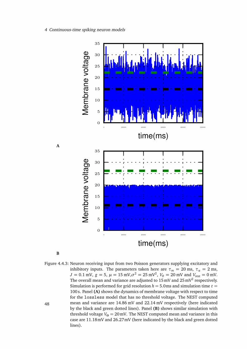
Figure 4.4.3: Neuron receiving input from two Poisson generators supplying excitatory andinhibitory inputs. The parameters taken here are τm = 20 ms, τα = 2 ms,J = 0.1 mV, g = 5, µ = 15 mV,σ2 = 25 mV2, Vθ = 20 mV and Vrest = 0 mV.The overall mean and variance are adjusted to 15mV and 25mV2 respectively.Simulation is performed for grid resolution h= 5.0ms and simulation time t =100 s. Panel (A) shows the dynamics of membrane voltage with respect to timefor the lossless model that has no threshold voltage. The NEST computedmean and variance are 14.86 mV and 22.14 mV respectively (here indicatedby the black and green dotted lines). Panel (B) shows similar simulation withthreshold voltage VΘ = 20mV. The NEST computed mean and variance in thiscase are 11.18mV and 26.27mV (here indicated by the black and green dottedlines).
48
4.5 Efficiency of spike test
The NEST computed mean agrees almost exactly with the pre-set mean value in case (A)where there is no threshold set. However, in case (B) we observe a large deviation in thevalue of the NEST computed mean from the pre-set mean. This is attributed to the fact thatwhenever the voltage hits threshold, it is reset back to the resting voltage (here 0 mV) andthis reset due to spiking also influences the overall dynamics of the network as seen closelyin 4.4.4. This is not the case when there is no threshold set, which validates exactly theresults observed analytically using the Campbell’s theorem as observed in 4.4.18.
1500 1520 1540 1560 1580 1600
time(ms)
0
5
10
15
20
25
Mem
bran
evo
ltage
NEST meanNEST variance
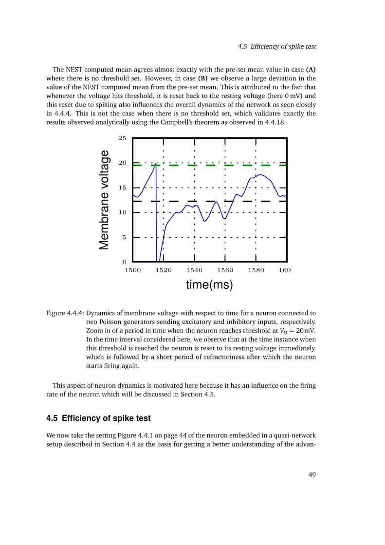
Figure 4.4.4: Dynamics of membrane voltage with respect to time for a neuron connected totwo Poisson generators sending excitatory and inhibitory inputs, respectively.Zoom in of a period in time when the neuron reaches threshold at VΘ = 20mV.In the time interval considered here, we observe that at the time instance whenthis threshold is reached the neuron is reset to its resting voltage immediately,which is followed by a short period of refractoriness after which the neuronstarts firing again.
This aspect of neuron dynamics is motivated here because it has an influence on the firingrate of the neuron which will be discussed in Section 4.5.
4.5 Efficiency of spike test
We now take the setting Figure 4.4.1 on page 44 of the neuron embedded in a quasi-networksetup described in Section 4.4 as the basis for getting a better understanding of the advan-
49
4 Continuous-time spiking neuron models
tages and limitations of including the additional spike test function Algorithm 4 onpage 38.
A
10 12 14 16 18 20 22 24 26 28 30
Mean voltage(mV)
0
5
10
15
20
25
30
Firin
gra
te
B
10 12 14 16 18 20 22 24 26 28 30
Mean voltage(mV)
0
20
40
60
80
100
120
140
Spi
kem
isse
s
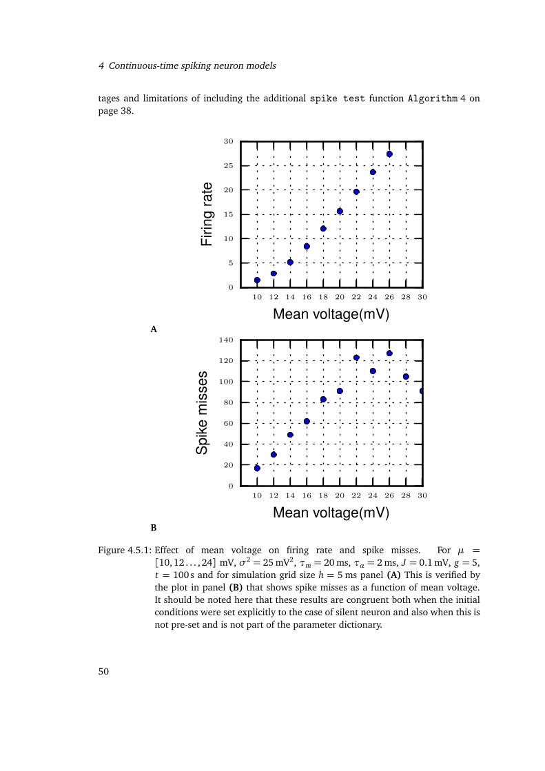
Figure 4.5.1: Effect of mean voltage on firing rate and spike misses. For µ =[10, 12 . . . , 24] mV, σ2 = 25 mV2, τm = 20 ms, τα = 2 ms, J = 0.1 mV, g = 5,t = 100s and for simulation grid size h = 5 ms panel (A) This is verified bythe plot in panel (B) that shows spike misses as a function of mean voltage.It should be noted here that these results are congruent both when the initialconditions were set explicitly to the case of silent neuron and also when this isnot pre-set and is not part of the parameter dictionary.
50
4.5 Efficiency of spike test
Figure 4.5.1 on page 50 panel (A) illustrates that for increasing mean voltage the fir-ing rate also increases which leads to the natural conclusion that spike misses also show ageneral rising trend with increase in mean voltage. This supports the rationale that for in-creasing mean voltage the chance that the voltage hits the threshold (here VΘ = 20mV) alsoincreases. Intuitively one would suppose that since the firing rate increases with increasein mean voltage, the number of missed spikes will also increase monotonically. This is sup-ported by panel (B) in Figure 4.5.1 on page 50. Up to 20 mV (the threshold voltage) wesee that the number of spike misses adopt a linear trend. At this point there are 91 spikesthat are missed within a simulation of duration t = 100sec. For mean voltage of 22 mVwe see a sudden increase of the number of misses to 123 and the trend goes up and dropsdown again to 127 at 26 mV. How does one explain the sudden increase in spike misses at22 mV? This is because the threshold VΘ is set to a standard value of 20 mV. To check ifthis hypothesis is true, the threshold was set to a lower value (10 mV) it was verified (datanot shown) that the number of spike misses exhibit a similar increase immediately after themembrane potential crosses threshold. The conclusion that we would draw here is that asa consequence of increasing mean voltage, firing rate and number of spike misses increasesfor a fixed simulation time and grid size. This motivates the investigation of effect of gridsize on firing rate. For fine grid resolutions, the canonical and lossless model shouldshow similar trends in firing rate. Ideally, there should be no spikes that are missed at thislevel of resolution.
51
4 Continuous-time spiking neuron models
A
10 12 14 16 18 20 22 24 26
Mean voltage (mV)
0
5
10
15
20
25
30
35
Firin
gra
te
canonicallossless
B
10 12 14 16 18 20 22 24 26
Mean voltage (mV)
0
5
10
15
20
25
30
35
Firin
gra
te
canonicallossless
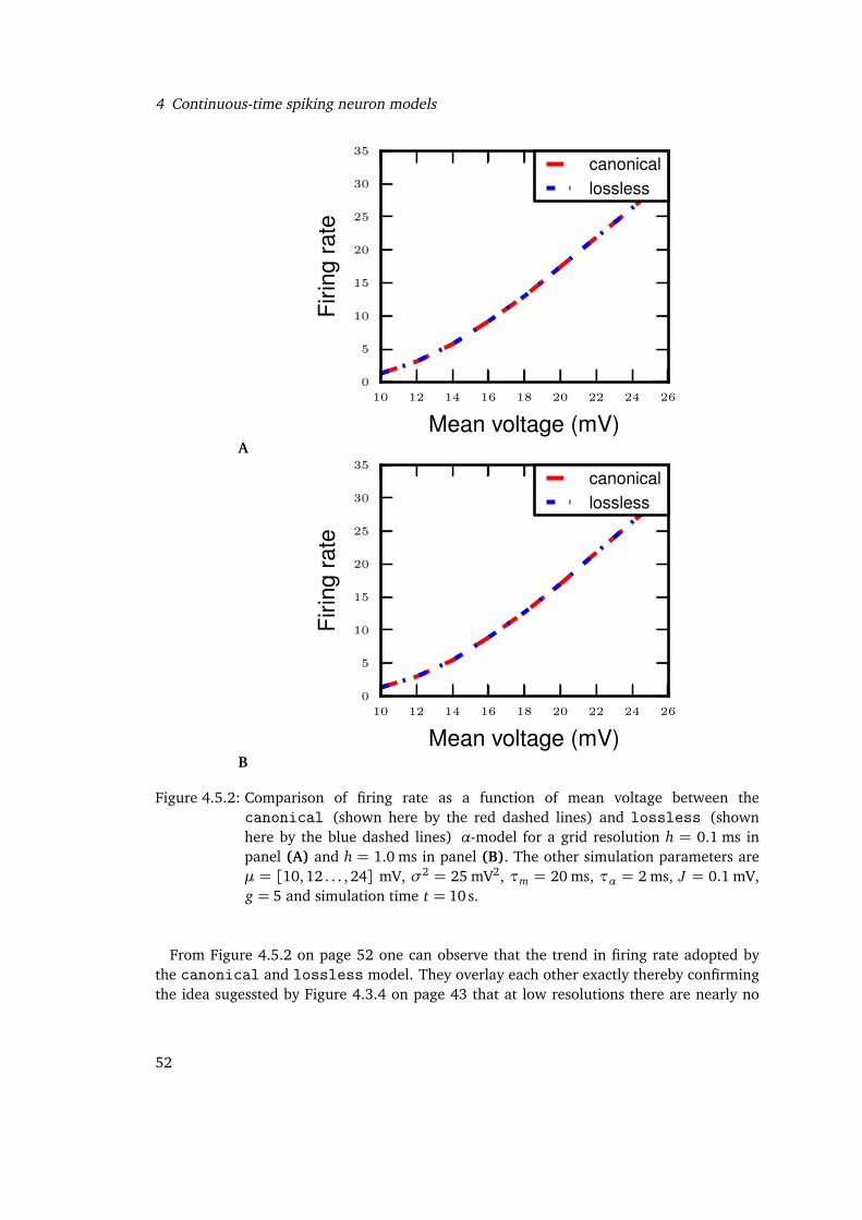
Figure 4.5.2: Comparison of firing rate as a function of mean voltage between thecanonical (shown here by the red dashed lines) and lossless (shownhere by the blue dashed lines) α-model for a grid resolution h = 0.1 ms inpanel (A) and h = 1.0 ms in panel (B). The other simulation parameters areµ = [10, 12 . . . , 24] mV, σ2 = 25 mV2, τm = 20 ms, τα = 2 ms, J = 0.1 mV,g = 5 and simulation time t = 10 s.
From Figure 4.5.2 on page 52 one can observe that the trend in firing rate adopted bythe canonical and lossless model. They overlay each other exactly thereby confirmingthe idea sugessted by Figure 4.3.4 on page 43 that at low resolutions there are nearly no
52
4.5 Efficiency of spike test
(∼ 7) spike misses. At this grid resolution, using the canonical model is rational. Now wewould like to observe the trend in firing rates of the canonical and lossless model forcoarser grid resolutions.
A
10 12 14 16 18 20 22 24 26
Mean voltage (mV)
0
5
10
15
20
25
30
Firin
gra
tecanonicallossless
B
10.0 10.2 10.4 10.6 10.8 11.0
Mean voltage (mV)
1.0
1.2
1.4
1.6
1.8
2.0
Firin
gra
te
canonicallossless
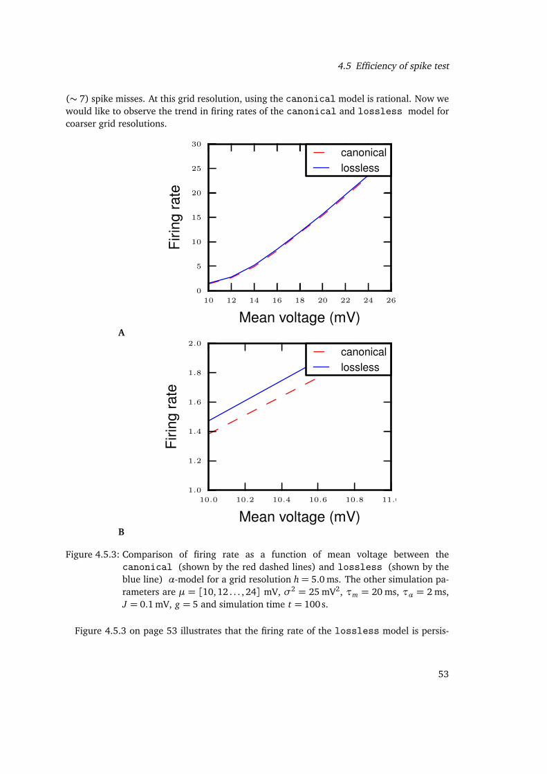
Figure 4.5.3: Comparison of firing rate as a function of mean voltage between thecanonical (shown by the red dashed lines) and lossless (shown by theblue line) α-model for a grid resolution h= 5.0 ms. The other simulation pa-rameters are µ = [10,12 . . . , 24] mV, σ2 = 25 mV2, τm = 20 ms, τα = 2 ms,J = 0.1 mV, g = 5 and simulation time t = 100 s.
Figure 4.5.3 on page 53 illustrates that the firing rate of the lossless model is persis-
53

4 Continuous-time spiking neuron models
tently above that of the canonical model, suggesting that this is because the spikes missedby the canonical model for higher resolutions are captured by the lossless model. Fig-ure 4.5.3 on page 53 Panel (A) shows that there is a small but distinguishable differencebetween the firing rate trend of the canonical and lossless model which can be caughtbetter in panel (B), where we observe that this is ∼ 0.2 Hz. This difference in firing ratecorresponds to ∼ 50 spike misses as can be verified in Figure 4.5.5 on page 56. Here wedraw attention to the observation made from Figure 4.4.4 on page 49, where the aspectthat the membrane voltage is reset immediately to the resting voltage whenever it hits thethreshold was discussed. Continuous voltage resets after spiking also influences firing rate.
54
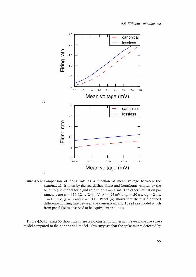
4.5 Efficiency of spike test
A
10 12 14 16 18 20 22 24 26
Mean voltage (mV)
0
5
10
15
20
25
Firin
gra
te
canonicallossless
B
16.0 16.5 17.0 17.5 18.0
Mean voltage (mV)
0
5
10
15
20
25
Firin
gra
te
canonicallossless
Figure 4.5.4: Comparison of firing rate as a function of mean voltage between thecanonical (shown by the red dashed lines) and lossless (shown by theblue line) α-model for a grid resolution h= 5.0 ms. The other simulation pa-rameters are µ = [10,12 . . . , 24] mV, σ2 = 25 mV2, τm = 20 ms, τα = 2 ms,J = 0.1 mV, g = 5 and t = 100 s. Panel (A) shows that there is a defineddifference in firing rate between the canonical and lossless model whichfrom panel (B) is observed to be equivalent to ∼ 4 Hz.
Figure 4.5.4 on page 55 shows that there is a consistently higher firing rate in the losslessmodel compared to the canonical model. This suggests that the spike misses detected by
55
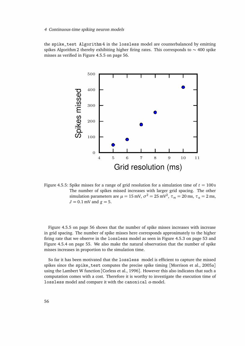
4 Continuous-time spiking neuron models
the spike_test Algorithm 4 in the lossless model are counterbalanced by emittingspikes Algorithm 2 thereby exhibiting higher firing rates. This corresponds to ∼ 400 spikemisses as verified in Figure 4.5.5 on page 56.
4 5 6 7 8 9 10 11
Grid resolution (ms)
0
100
200
300
400
500
Spi
kes
mis
sed
Figure 4.5.5: Spike misses for a range of grid resolution for a simulation time of t = 100 sThe number of spikes missed increases with larger grid spacing. The othersimulation parameters are µ = 15 mV, σ2 = 25 mV2, τm = 20 ms, τα = 2 ms,J = 0.1 mV and g = 5.
Figure 4.5.5 on page 56 shows that the number of spike misses increases with increasein grid spacing. The number of spike misses here corresponds approximately to the higherfiring rate that we observe in the lossless model as seen in Figure 4.5.3 on page 53 andFigure 4.5.4 on page 55. We also make the natural observation that the number of spikemisses increases in proportion to the simulation time.
So far it has been motivated that the lossless model is efficient to capture the missedspikes since the spike_test computes the precise spike timing [Morrison et al., 2005a]using the Lambert W function [Corless et al., 1996]. However this also indicates that such acomputation comes with a cost. Therefore it is worthy to investigate the execution time oflossless model and compare it with the canonical α-model.
56
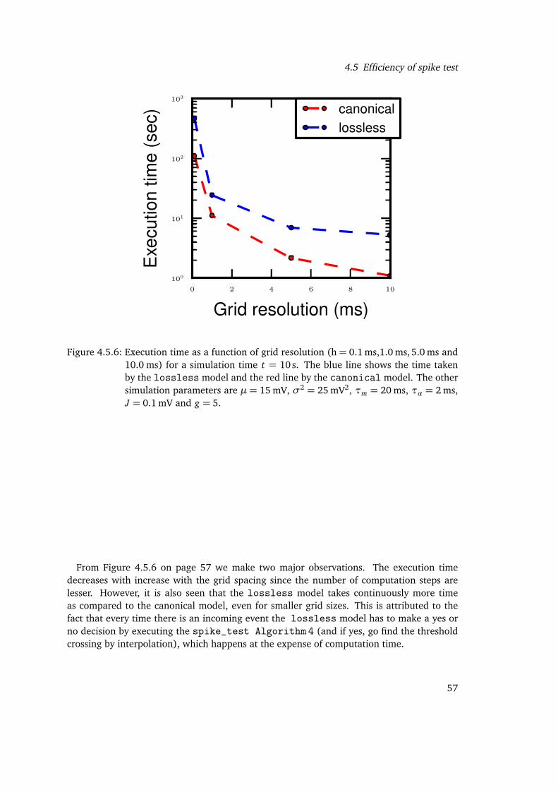
4.5 Efficiency of spike test
0 2 4 6 8 10
Grid resolution (ms)
100
101
102
103
Exe
cutio
ntim
e(s
ec) canonical
lossless
Figure 4.5.6: Execution time as a function of grid resolution (h= 0.1 ms,1.0 ms,5.0 ms and10.0 ms) for a simulation time t = 10s. The blue line shows the time takenby the lossless model and the red line by the canonical model. The othersimulation parameters are µ = 15 mV, σ2 = 25 mV2, τm = 20 ms, τα = 2 ms,J = 0.1 mV and g = 5.
From Figure 4.5.6 on page 57 we make two major observations. The execution timedecreases with increase with the grid spacing since the number of computation steps arelesser. However, it is also seen that the lossless model takes continuously more timeas compared to the canonical model, even for smaller grid sizes. This is attributed to thefact that every time there is an incoming event the lossless model has to make a yes orno decision by executing the spike_test Algorithm 4 (and if yes, go find the thresholdcrossing by interpolation), which happens at the expense of computation time.
57
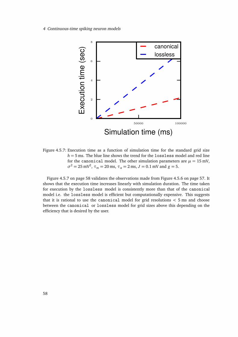
4 Continuous-time spiking neuron models
50000 100000
Simulation time (ms)
0
2
4
6
8
Exe
cutio
ntim
e(s
ec) canonical
lossless
Figure 4.5.7: Execution time as a function of simulation time for the standard grid sizeh= 5 ms. The blue line shows the trend for the lossless model and red linefor the canonical model. The other simulation parameters are µ = 15 mV,σ2 = 25 mV2, τm = 20 ms, τα = 2 ms, J = 0.1 mV and g = 5.
Figure 4.5.7 on page 58 validates the observations made from Figure 4.5.6 on page 57. Itshows that the execution time increases linearly with simulation duration. The time takenfor execution by the lossless model is consistently more than that of the canonicalmodel i.e. the lossless model is efficient but computationally expensive. This suggeststhat it is rational to use the canonical model for grid resolutions < 5 ms and choosebetween the canonical or lossless model for grid sizes above this depending on theefficiency that is desired by the user.
58
5 Discussion
The lossless model is the accurate implementation of the mathematical model describingthe LIF neuron with α-PSCs. The model is efficient and can catch otherwise missed spikesin coarse grid resolutions Figure 4.5.5 on page 56. Since the lossless model never loosesspikes its accuracy is always above that of the canonical model. We also observe fromthe comparison of execution time between the two modelsFigure 4.5.7 on page 58 that thisaccuracy comes with computational cost.
However, it is rational to compare the execution time of two models that have equivalentaccuracy which was not the case in our preliminary analysis here. Therefore a comparisonof the canonical α-model with a pre-set tolerance level for spike misses with that of thelossless α-model would give us a better insight into the efficiency of the new model.
A detailed analysis of the state variables governing the system of equations of the modelcould help us exclude more initial conditions that correspond to the situation where therecan be no spike misses, thereby optimizing the spike test function and improving theefficiency of the lossless model.
59

Bibliography
Rajagopal Ananthanarayanan and Dharmendra S. Modha. Anatomy of a cortical simula-tor. In Supercomputing 2007: Proceedings of the ACM/IEEE SC2007 Conference on HighPerformance Networking and Computing, New York, NY, 2007. Association for ComputingMachinery.
C. Bernard, Y. C. Ge, E. Stockley, J. B. Willis, and H. V. Wheal. Synaptic integration ofNMDA and non-NMDA receptors in large neuronal network models solved by means ofdifferential equations. Biological Cybernetics, 70:267–273, 1994.
Norman Campbell. The study of discontinuous phenomena. ProcCambridgePhilSoc, 15:117–136, 1909.
R. M. Corless, G. H. Gonnet, D. E. G. Hare, D. J. Jeffrey, and D. E. Knuth. On the lambert wfunction. Advances in Computational Mathematics, 5:329–359, 1996.
Markus Diesmann and Marc-Oliver Gewaltig. NEST: An environment for neural systemssimulations. In Theo Plesser and Volker Macho, editors, Forschung und wisschenschaftlichesRechnen, Beiträge zum Heinz-Billing-Preis 2001, volume 58 of GWDG-Bericht, pages 43–70.Ges. für Wiss. Datenverarbeitung, Göttingen, 2002.
Markus Diesmann, Marc-Oliver Gewaltig, Stefan Rotter, and Ad Aertsen. State space analysisof synchronous spiking in cortical neural networks. Neurocomputing, 38–40:565–571,2001.
Mikael Djurfeldt. Large-scale Simulation of Neuronal Systems. PhD thesis, KTH School ofComputer Science and Communication, Stockholm, Sweden, 2009.
J. M. Eppler, M. Helias, E. Muller, M. Diesmann, and M. Gewaltig. PyNEST: a convenientinterface to the NEST simulator. 2:12, 2009.
Alois Ferscha. Parallel and distributed simulation of discrete event systems. In Albert Y.Zomaya, editor, Parallel and Distributed Computing Handbook, chapter 35, pages 1003–1041. McGraw-Hill, 1996.
Richard M. Fujimoto. Parallel and distributed simulation systems. Wiley, New York, 2000.ISBN 0-471-18383-0.
Marc-Oliver Gewaltig and Markus Diesmann. NEST (NEural Simulation Tool). Scholarpedia,2(4):1430, 2007.
61
Bibliography
Sven Goedeke and Markus Diesmann. The mechanism of synchronization in feed-forwardneuronal networks. 10:015007, 2008.
D. F. M. Goodman and R. Brette. The Brian simulator. 3(2):192–197, 2009. doi:10.3389/neuro.01.026.2009.
D. Hansel, G. Mato, C. Meunier, and L. Neltner. On numerical simulations of integrate-and-fire neural networks. Neural Computation, 10(2):467–483, Feb., 15 1998.
Moritz Helias, Tom Tetzlaff, and Markus Diesmann. Echoes in correlated neural systems.15:023002, 2013.
Michael Hines. NEURON — a program for simulation of nerve equations. In F. Eeckman, ed-itor, Neural Systems: Analysis and Modeling, pages 127–136. Kluwer Academic Publishers,Norwell, Ma, 1993.
Susanne Kunkel, Moritz Helias, Markus Diesmann, and Abigail Morrison. Fail-safe detectionof threshold crossings of linear integrate-and-fire neuron models in time-driven simula-tions. BMC Neuroscience, 12(Suppl 1):P229, 2011.
A. Morrison, A. Aertsen, and M. Diesmann. Spike-timing dependent plasticity in balancedrandom networks. Neural Computation, 19:1437–1467, 2007a.
A. Morrison and M. Diesmann. Maintaining causality in discrete time neuronal networksimulations. In P. beim Graben, C. Zhou, M. Thiel, and J. Kurths, editors, Lectures inSupercomputational Neuroscience: Dynamics in Complex Brain Networks, UnderstandingComplex Systems, pages 267–278. Springer, 2008.
Abigail Morrison, Johan Hake, Sirko Straube, Hans Ekkehard Plesser, and Markus Dies-mann. Precise spike timing with exact subthreshold integration in discrete time networksimulations. In Proceedings of the 30th Göttingen Neurobiology Conference, page 205B,2005a.
Abigail Morrison, Carsten Mehring, Theo Geisel, Ad Aertsen, and Markus Diesmann. Ad-vancing the boundaries of high connectivity network simulation with distributed comput-ing. Neural Computation, 17(8):1776–1801, 2005b.
Abigail Morrison, Sirko Straube, Hans Ekkehard Plesser, and Markus Diesmann. Exact sub-threshold integration with continuous spike times in discrete time neural network simu-lations. Neural Computation, 19(1):47–79, 2007b.
H. E. Plesser and M. Diesmann. Simplicity and efficiency of integrate-and-fire neuron mod-els. Neural Computation, 21:353–359, 2009.
Python Software Foundation. The Python programming language, 2008.http://www.python.org.
62
Bibliography
A. Rauch, G. La Camera, H. Lüscher, W. Senn, and S. Fusi. Neocortical pyramidal cellsrespond as integrate-and-fire neurons to in vivo like input currents. Journal of Neurophys-iology, 90:1598–1612, 2003.
Stefan Rotter and Markus Diesmann. Exact digital simulation of time-invariant linear sys-tems with applications to neuronal modeling. Biological Cybernetics, 81(5/6):381–402,1999.
M. J. Shelley and L. Tao. Efficient and accurate time-stepping schemes for integrate-and-fireneuronal networks. Journal of Computational Neuroscience, 11(2):111–119, 2001.
A. Sloot, J. A. Kaandorp, G. Hoekstra, and B. J. Overeinder. Distributed simulation withcellular automata: Architecture and applications. In J. Pavelka, G. Tel, and M. Bartosek,editors, SOFSEM’99, LNCS, pages 203–248, Berlin, Heidelberg, 1999. Springer-Verlag.
Matthew A. Wilson and James M. Bower. The simulation of large-scale neural networks.In Christof Koch and Idan Segev, editors, Methods in Neuronal Modeling: From Synapsesto Networks, chapter 9, pages 291–333. A Bradford Book, The MIT Press, Cambridge,Massachusetts, 1989.
Bernard P. Zeigler, Herbert Praehofer, and Tag Gon Kim. Theory of Modeling and Simulation:Integrating Discrete Event and Continuous Complex Dynamic Systems. Academic Press,Amsterdam, 2 edition, 2000.
63