DEPARTMENT OF INFORMATICS M.Sc. IN COMPUTER …nlp.cs.aueb.gr/theses/brokos_msc_thesis.pdf · al.,...
48
DEPARTMENT OF INFORMATICS M.Sc. IN COMPUTER SCIENCE M.Sc. Thesis “Document Reranking with Deep Learning in Information Retrieval” Georgios-Ioannis Brokos ΕΥ1615 Supervisors: Ion Androutsopoulos Ryan McDonald ATHENS, JUNE 2018
Transcript of DEPARTMENT OF INFORMATICS M.Sc. IN COMPUTER …nlp.cs.aueb.gr/theses/brokos_msc_thesis.pdf · al.,...
DEPARTMENT OF INFORMATICS
M.Sc. IN COMPUTER SCIENCE
M.Sc. Thesis
“Document Reranking with Deep Learning in Information Retrieval”
Georgios-Ioannis Brokos
ΕΥ1615
Supervisors: Ion Androutsopoulos
Ryan McDonald
ATHENS, JUNE 2018

i
Acknowledgements
I would like to thank my supervisor Ion Androutsopoulos for his continuous guidance andsupport, as well as my second supervisor Ryan McDonald for his valuable help and ideas thatformed much of the content of this thesis.
I would also like to thank the members of AUEB’s Natural Language Processing group, espe-cially Dimitris Pappas and Polyvios Liosis for the discussions and ideas that we exchanged onour closely related works.
A special thanks goes to Makis Malakasiotis for his help and guidance during my – relevant tothis work – B.Sc. thesis and Giannos Koutsikakis for the great cooperation and useful discus-sions that we had throughout our M.Sc. studies.
Finally, a big thanks goes to my family for their continuous support and patience.
ii
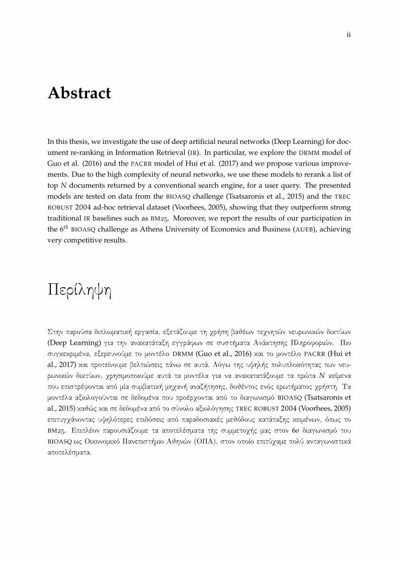
Abstract
In this thesis, we investigate the use of deep artificial neural networks (Deep Learning) for doc-ument re-ranking in Information Retrieval (IR). In particular, we explore the DRMM model ofGuo et al. (2016) and the PACRR model of Hui et al. (2017) and we propose various improve-ments. Due to the high complexity of neural networks, we use these models to rerank a list oftop N documents returned by a conventional search engine, for a user query. The presentedmodels are tested on data from the BIOASQ challenge (Tsatsaronis et al., 2015) and the TREC
ROBUST 2004 ad-hoc retrieval dataset (Voorhees, 2005), showing that they outperform strongtraditional IR baselines such as BM. Moreover, we report the results of our participation inthe 6th BIOASQ challenge as Athens University of Economics and Business (AUEB), achievingvery competitive results.
Περίληψη
Στην παρούσα διπλωματική εργασία, εξετάζουμε τη χρήση βαθέων τεχνητών νευρωνικών δικτύων
(Deep Learning) για την ανακατάταξη εγγράφων σε συστήματα Ανάκτησης Πληροφοριών. Πιοσυγκεκριμένα, εξερευνούμε το μοντέλο DRMM (Guo et al., 2016) και το μοντέλο PACRR (Hui etal., 2017) και προτείνουμε βελτιώσεις πάνω σε αυτά. Λόγω της υψηλής πολυπλοκότητας των νευ-ρωνικών δικτύων, χρησιμοποιούμε αυτά τα μοντέλα για να ανακατατάξουμε τα πρώτα N κείμεναπου επιστρέφονται από μία συμβατική μηχανή αναζήτησης, δοθέντος ενός ερωτήματος χρήστη. Τα
μοντέλα αξιολογούνται σε δεδομένα που προέρχονται από το διαγωνισμό BIOASQ (Tsatsaronis etal., 2015) καθώς και σε δεδομένα από το σύνολο αξιολόγησης TREC ROBUST 2004 (Voorhees, 2005)επιτυγχάνοντας υψηλότερες επιδόσεις από παραδοσιακές μεθόδους κατάταξης κειμένων, όπως το
BM. Επιπλέον παρουσιάζουμε τα αποτελέσματα της συμμετοχής μας στον 6o διαγωνισμό τουBIOASQ ως Οικονομικό Πανεπιστήμιο Αθηνών (ΟΠΑ), στον οποίο επιτύχαμε πολύ ανταγωνιστικά
αποτελέσματα.
iii
Contents
1 Introduction 11.1 The ad-hoc retrieval task . . . . . . . . . . . . . . . . . . . . . . . . . . . . . . . . . 11.2 The goal of the thesis . . . . . . . . . . . . . . . . . . . . . . . . . . . . . . . . . . . 21.3 Outline . . . . . . . . . . . . . . . . . . . . . . . . . . . . . . . . . . . . . . . . . . . 4
2 Methods 52.1 The BM25 scoring function . . . . . . . . . . . . . . . . . . . . . . . . . . . . . . . . 52.2 Neural network architectures for document relevance ranking . . . . . . . . . . . 62.3 The DRMM model . . . . . . . . . . . . . . . . . . . . . . . . . . . . . . . . . . . . 72.4 The PACRR model . . . . . . . . . . . . . . . . . . . . . . . . . . . . . . . . . . . . 102.5 Extra features for exact match capturing . . . . . . . . . . . . . . . . . . . . . . . . 13
3 Experiments 153.1 Data . . . . . . . . . . . . . . . . . . . . . . . . . . . . . . . . . . . . . . . . . . . . . 15
3.1.1 BioASQ dataset . . . . . . . . . . . . . . . . . . . . . . . . . . . . . . . . . . 153.1.2 TREC Robust2004 dataset . . . . . . . . . . . . . . . . . . . . . . . . . . . . 22
3.2 Evaluation Measures . . . . . . . . . . . . . . . . . . . . . . . . . . . . . . . . . . . 243.3 Experimental Setup . . . . . . . . . . . . . . . . . . . . . . . . . . . . . . . . . . . . 27
3.3.1 Initial document retrieval . . . . . . . . . . . . . . . . . . . . . . . . . . . . 273.3.2 Document reranking with neural networks . . . . . . . . . . . . . . . . . . 27
3.4 Ideal reranking . . . . . . . . . . . . . . . . . . . . . . . . . . . . . . . . . . . . . . 293.5 Experimental results . . . . . . . . . . . . . . . . . . . . . . . . . . . . . . . . . . . 29
3.5.1 BioASQ experiments . . . . . . . . . . . . . . . . . . . . . . . . . . . . . . . 293.5.2 TREC Robust 2004 experiments . . . . . . . . . . . . . . . . . . . . . . . . . 34
4 Related Work 36
5 Conclusions and future work 385.1 Conclusions . . . . . . . . . . . . . . . . . . . . . . . . . . . . . . . . . . . . . . . . 385.2 Future Work . . . . . . . . . . . . . . . . . . . . . . . . . . . . . . . . . . . . . . . . 38
Appendix A 40
Bibliography 42
1
Chapter 1
Introduction
1.1 The ad-hoc retrieval task
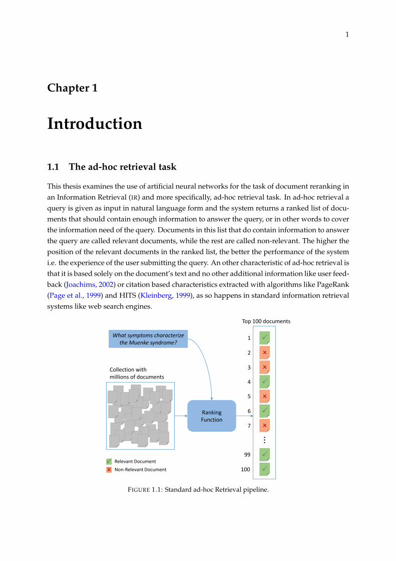
This thesis examines the use of artificial neural networks for the task of document reranking inan Information Retrieval (IR) and more specifically, ad-hoc retrieval task. In ad-hoc retrieval aquery is given as input in natural language form and the system returns a ranked list of docu-ments that should contain enough information to answer the query, or in other words to coverthe information need of the query. Documents in this list that do contain information to answerthe query are called relevant documents, while the rest are called non-relevant. The higher theposition of the relevant documents in the ranked list, the better the performance of the systemi.e. the experience of the user submitting the query. An other characteristic of ad-hoc retrieval isthat it is based solely on the document’s text and no other additional information like user feed-back (Joachims, 2002) or citation based characteristics extracted with algorithms like PageRank(Page et al., 1999) and HITS (Kleinberg, 1999), as so happens in standard information retrievalsystems like web search engines.
What symptoms characterize the Muenke syndrome?
Ranking Function
...
Top 100 documents
1
2
3
4
5
6
7
99
100
Collection with millions of documents
Relevant Document
Non-Relevant Document
FIGURE 1.1: Standard ad-hoc Retrieval pipeline.
Chapter 1. Introduction 2
Figure 1.1 shows the standard pipeline of an ad-hoc retrieval system. A large collection isavailable, usually containing millions of documents. The most important component of thesystem is the ranking function. Given a query from a user, the ranking function calculatesa relevance score between the query and each one of the documents in the collection. Then,documents are sorted by decreasing relevance score and the top N in the list are shown tothe user. A typical example of a ranking function is Query Likelihood (QL) which builds alanguage model for each document in the collection and then scores each document by theprobability assigned to the query by the document’s language model (Ponte and Croft, 1998).Ranking functions based on Term Frequency (TF) and Inverse Document Frequency (IDF) arealso widely used in information retrieval. A TF-IDF based ranking function that has gainedpopularity in traditional information retrieval is BM (Robertson et al., 1995). Among otherimprovements, it differs from a common TF-IDF model in the fact that it takes into accountthe document length in order to avoid being affected by highly varied document lengths in acollection.
1.2 The goal of the thesis
The main limitation of traditional information retrieval models like QL and BM is that theyare based on exact word matching (i.e., common words between a query and a document).Techniques like stemming are used to match words based on the word root, in order to increaseword matching, however problems like synonymity are not tackled. Also polysemy can not bedetected since these models are not context aware.
In the last few years, multi-dimensional dense word representations (word embeddings)produced by shallow neural networks (Mikolov et al., 2013; Pennington et al., 2014) havegained much popularity and are widely used in various Natural Language Processing (NLP)tasks. Their basic characteristic is that the representations of syntactically or semantically sim-ilar words are close to each other in this multi-dimensional space. For example the words painand ache have similar dense representations in this model, where these two words would betotally different in a conventional IR system relying on exact term matching. In a previouswork we have examined the use of word embeddings for information retrieval in order to uti-lize their benefits, by using centroids of word embeddings to represent queries and documentsand then applying a simple similarity metric on these representations as well as a rerankingfilter that operates directly on word embeddings (Brokos, Malakasiotis, and Androutsopoulos,2016). However, traditional IR systems like BM seemed to outperform this approach.
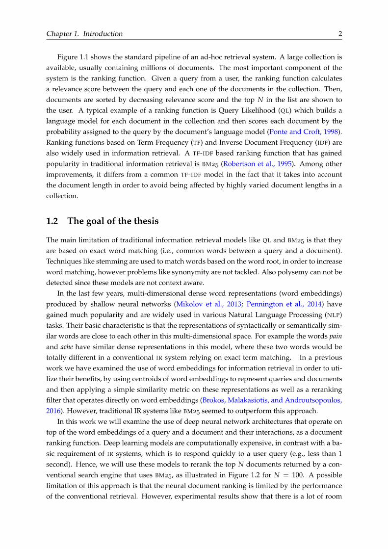
In this work we will examine the use of deep neural network architectures that operate ontop of the word embeddings of a query and a document and their interactions, as a documentranking function. Deep learning models are computationally expensive, in contrast with a ba-sic requirement of IR systems, which is to respond quickly to a user query (e.g., less than 1second). Hence, we will use these models to rerank the top N documents returned by a con-ventional search engine that uses BM, as illustrated in Figure 1.2 for N = 100. A possiblelimitation of this approach is that the neural document ranking is limited by the performanceof the conventional retrieval. However, experimental results show that there is a lot of room
Chapter 1. Introduction 3
What symptoms characterize the Muenke syndrome?
InitialBM25 Retrieval
Deep relevance reranking
...
...Top 100 documents Top 100 documents
1
2
3
4
5
6
7
99
100
1
2
3
4
5
6
7
Relevant Document
Non-Relevant Document
99
100
Collection with millions of documents
FIGURE 1.2: Ad-hoc retrieval with deep relevance document reranking.
for improvement in the ranking of the list returned by BM, i.e., there are many relevant doc-uments but in low (bad) positions.
More specifically, we will use and improve two recently proposed document relevanceranking models, the Deep Relevance Matching Model of Guo et al., 2016 and the Position-Aware Convolutional-Recurrent Relevance matching model of Hui et al., 2017 using also im-provements proposed by the aforementioned authors (Hui et al., 2018). We test the models ondata from the BIOASQ challenge (Tsatsaronis et al., 2015) and the TREC ROBUST 2004 ad-hocretrieval dataset (Voorhees, 2005). Experimental results show that the proposed models, com-bined with a set of additional exact term matching features, outperform traditional BM basedbaselines.1
Moreover, we report the results of our participation in the document retrieval task of the6th year of the BIOASQ challenge, using the model that performed best on development data,showing that it achieves competitive results, usually outperformed only by other deep learn-ing methods based or inspired by the presented models, submitted by our team as AthensUniversity of Economics and Business (AUEB).
1The code and data used for the experiments of this thesis are available at: https://github.com/gbrokos/document-reranking-with-deep-learning-in-ir
Chapter 1. Introduction 4
1.3 Outline
The rest of the thesis is organized as follows:
• Chapter 2 - Description of the BM retrieval model and the deep learning rerankingmodels.
• Chapter 3 - Description of the datasets used and the experimental setup, along with pre-sentation of the experimental results.
• Chapter 4 - Discussion about recent work related to document ranking.
• Chapter 5 - Discussion about the findings and contributions of the thesis, as well as ideasfor future work.
5
Chapter 2
Methods
This chapter describes methods that can be used to produce a relevance score rel(Q, D) for adocument D given a query Q. Starting with the BM baseline we move to the deep learningmodels that will be used to rerank the list of documents retrieved by BM. Finally, additionalfeatures capturing strong exact term matching signals are presented and integrated into thedeep learning models.
2.1 The BM25 scoring function
As already mentioned, we will utilize efficient retrieval frameworks (search engines) to reducethe number of documents for the neural network reranking models. BM (Robertson et al.,1995) is a scoring function that is widely used in many traditional search engines. Given aquery Q containing n terms q1, q2, . . . , qn and a document D, BM calculates a relevance scorebased on exact matching of word uni-grams between the query and the document as follows:
rel(Q, D) =n
∑i=1
IDF(qi) ·TF(qi, D) · (k1 + 1)
TF(qi, D) + k1 · (1− b + b · |D|avgDocLen )
(2.1)
where TF(qi) is the Term Frequency of the i-th query term in document D and IDF(qi) is theInverse Document Frequency of term qi (Eq. 2.2), |D| is the length of document D in tokensand avgDocLen is the average length of the documents in the corpus. Finally k1 and b areparameters to be tuned.
IDF is computed as follows:
IDF(qi) = log|D|
d f (qi) + 0.5(2.2)
where d f (qi) is the document frequency of the word qi, |D| is the total number of documents inthe corpus and 0.5 is a smoothing factor. As other TF-IDF based methods, BM relies on exactterm matching between the query and the document. However, BM is usually superior toother simpler TF-IDF methods, possibly due to its document length normalization factor.
Chapter 2. Methods 6
2.2 Neural network architectures for document relevance ranking
Neural networks for document relevance ranking often belong to one of the following cate-gories: representation-focused and interaction-focused models (Guo et al., 2016; Zhang et al.,2016).
...
...
...
...
...
...
Relevance Score
Query Document
Seperate representations for Query and Document
Inputs
...
...
...
Relevance Score
Query
Joint Query-Document representation
Inputs
Document
Joint representation
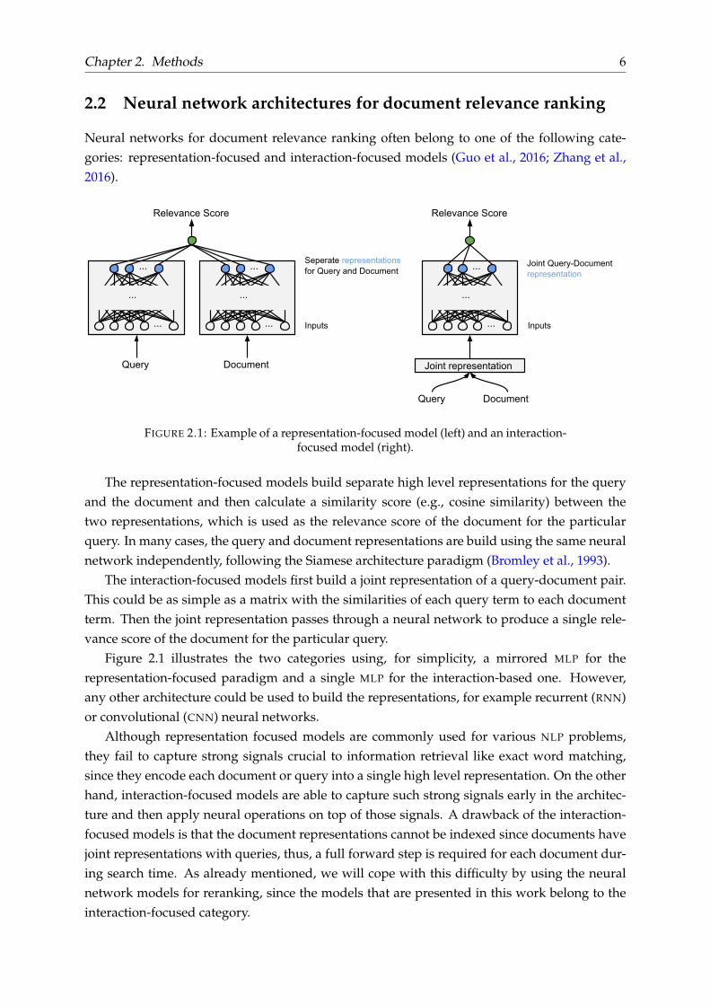
FIGURE 2.1: Example of a representation-focused model (left) and an interaction-focused model (right).
The representation-focused models build separate high level representations for the queryand the document and then calculate a similarity score (e.g., cosine similarity) between thetwo representations, which is used as the relevance score of the document for the particularquery. In many cases, the query and document representations are build using the same neuralnetwork independently, following the Siamese architecture paradigm (Bromley et al., 1993).
The interaction-focused models first build a joint representation of a query-document pair.This could be as simple as a matrix with the similarities of each query term to each documentterm. Then the joint representation passes through a neural network to produce a single rele-vance score of the document for the particular query.
Figure 2.1 illustrates the two categories using, for simplicity, a mirrored MLP for therepresentation-focused paradigm and a single MLP for the interaction-based one. However,any other architecture could be used to build the representations, for example recurrent (RNN)or convolutional (CNN) neural networks.
Although representation focused models are commonly used for various NLP problems,they fail to capture strong signals crucial to information retrieval like exact word matching,since they encode each document or query into a single high level representation. On the otherhand, interaction-focused models are able to capture such strong signals early in the architec-ture and then apply neural operations on top of those signals. A drawback of the interaction-focused models is that the document representations cannot be indexed since documents havejoint representations with queries, thus, a full forward step is required for each document dur-ing search time. As already mentioned, we will cope with this difficulty by using the neuralnetwork models for reranking, since the models that are presented in this work belong to theinteraction-focused category.
Chapter 2. Methods 7
Training Neural Networks for Information Retrieval
Training neural networks for document relevance ranking usually requires two forward prop-agations; one given as input a query q and a document d+ where d+ is relevant to the queryq and one given as input the same query q and a document d− not relevant to q. The neuralnetwork produces a relevance score rel(q, d+) for the first query-document pair (containing therelevant document) and a score rel(q, d−) for the second query-document pair (containing thenon-relevant document). Two kinds of loss functions can then be used:
Hinge loss: Minimizing hinge loss aims to separate by a margin the scores assigned tothe relevant and the non-relevant document given the same query, with the relevant documenthaving the highest score among the two. In Eq. 2.3, the margin is set to 1, which is common.
L(q, d+, d−; Θ) = max{0, 1− rel(q, d+) + rel(q, d−)} (2.3)
Negative log-loss: Minimizing negative log-loss aims to maximize the probability givento the relevant document that is obtained after applying a softmax function to rel(q, d+) andrel(q, d−).
L(q, d+, d−; Θ) = −log(
exp(rel(q, d+))exp(rel(q, d+)) + exp(rel(q, d−))
)(2.4)
The network parameters are then updated via a single backpropagation step, based on theselected loss.
2.3 The DRMM model
The Deep Relevance Matching Model (DRMM) of Guo et al., 2016, belongs to the interaction-focused category of document ranking neural networks, since it first calculates matching sig-nals between query-document term pairs which are then passed to neural operations that pro-duce a relevance score. DRMM takes as input a query q:
q = {w(q)1 , w(q)
2 , . . . , w(q)m } (2.5)
and a document d:
d = {w(d)1 , w(d)
2 , . . . , w(d)n } (2.6)
where w(q)i denotes the pre-trained word embedding of the i-th query term of a query with
length m and w(d)i is the pre-trained word embedding of the i-th query term of a query with
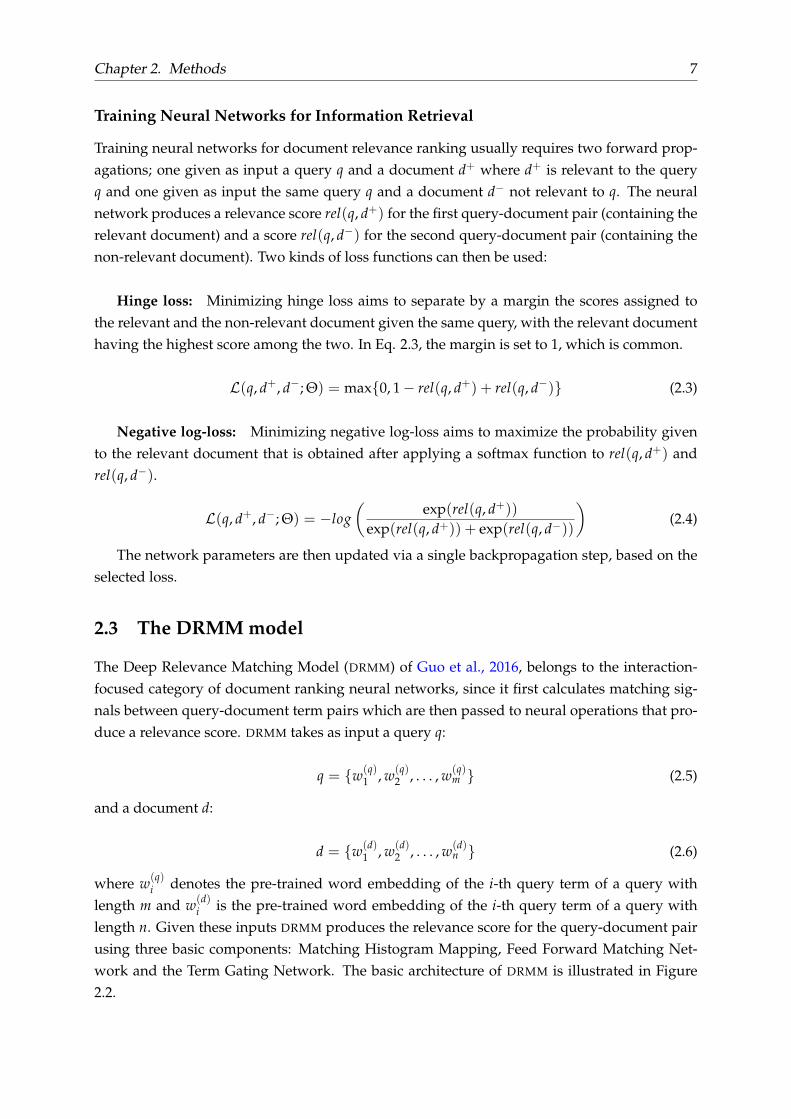
length n. Given these inputs DRMM produces the relevance score for the query-document pairusing three basic components: Matching Histogram Mapping, Feed Forward Matching Net-work and the Term Gating Network. The basic architecture of DRMM is illustrated in Figure2.2.
Chapter 2. Methods 8
Term Gating
q1 q2 q3
IDF(q1) IDF(q2) IDF(q3)
Revelance Score
Query Terms
Document Terms
...d1 d2 d3 dn
Matching Histograms
Feed Forward Matching
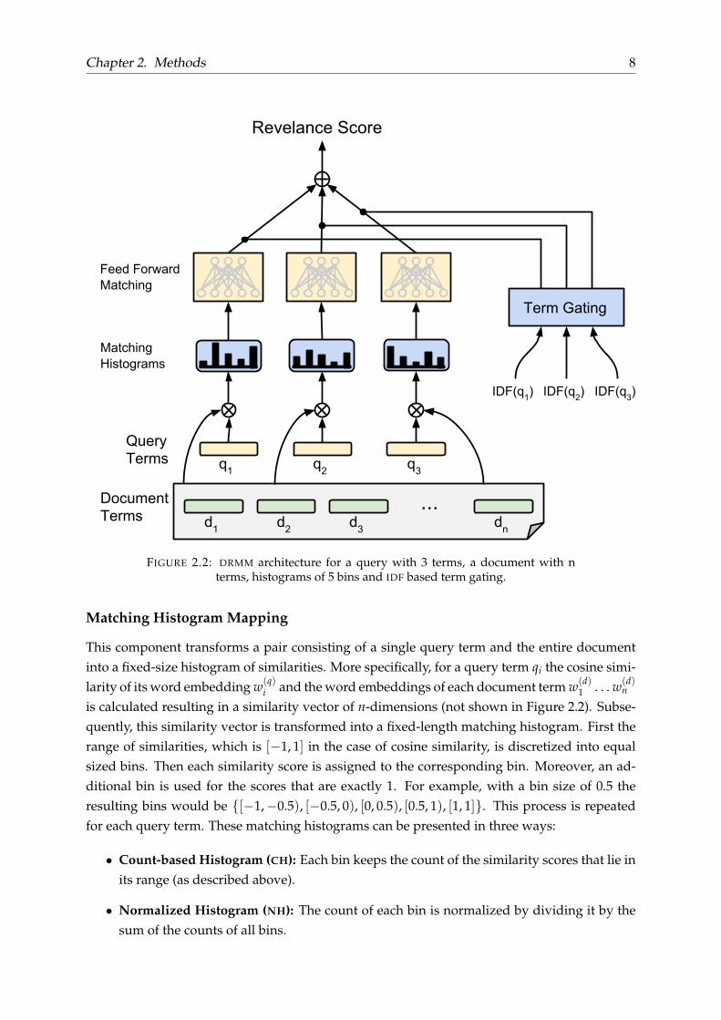
FIGURE 2.2: DRMM architecture for a query with 3 terms, a document with nterms, histograms of 5 bins and IDF based term gating.
Matching Histogram Mapping
This component transforms a pair consisting of a single query term and the entire documentinto a fixed-size histogram of similarities. More specifically, for a query term qi the cosine simi-larity of its word embedding w(q)
i and the word embeddings of each document term w(d)1 . . . w(d)
n
is calculated resulting in a similarity vector of n-dimensions (not shown in Figure 2.2). Subse-quently, this similarity vector is transformed into a fixed-length matching histogram. First therange of similarities, which is [−1, 1] in the case of cosine similarity, is discretized into equalsized bins. Then each similarity score is assigned to the corresponding bin. Moreover, an ad-ditional bin is used for the scores that are exactly 1. For example, with a bin size of 0.5 theresulting bins would be {[−1,−0.5), [−0.5, 0), [0, 0.5), [0.5, 1), [1, 1]}. This process is repeatedfor each query term. These matching histograms can be presented in three ways:
• Count-based Histogram (CH): Each bin keeps the count of the similarity scores that lie inits range (as described above).
• Normalized Histogram (NH): The count of each bin is normalized by dividing it by thesum of the counts of all bins.
Chapter 2. Methods 9
• LogCount-based Histogram (LCH): A logarithm is applied to the CH count of each bin.
Feed Forward Matching Network
Each query term matching histogram, then passes through a Multi-Layer Perceptron (the samefor all histograms), in order to produce a matching score for each query term.
Term Gating Network
At this point a simple summation of the query term matching scores could be used to pro-duce the query-document relevance score. However, DRMM deploys a term gating networkto weight each term matching score based on query term importance. There are two ways toproduce these gating weights gi, both using linear self-attention:
gi =exp (wT
g x(q)i )
∑Mj=1 exp (wT
g x(q)j )(2.7)
• Inverse Document Frequency (IDF): In the simplest case, x(q)i is the IDF of the i-th queryterm and wg is a single parameter (scalar weight).
• Term Vector (TV): In this case, x(q)i is the word embedding of the i-th query term and wg
is a weight vector of the same dimensionality.
Since experimental results of Guo et al., 2016 suggest that DRMM performs best using LogCount-based Histograms (LCH) and Inverse Document Frequency (IDF) term gating, only this setupof the model will be used (DRMMLCH×IDF) which for simplicity will be called DRMM.
Training
Having the relevance scores rel(q, d+), rel(q, d−) produced by the forward propagations for aquery q, a relevant document d+ and a non-relevant document d−, hinge-loss (Eq. 2.3) is thenapplied to these scores and the model’s parameters are updated via backpropagation using theAdam optimizer (Kingma and Ba, 2014).
Chapter 2. Methods 10
2.4 The PACRR model
Hui et al. (2017) proposed the Position-Aware Convolutional-Recurrent Relevance matchingmodel (PACRR), an interaction-focused neural network model which aims to capture position-dependent interactions between a query and a document.
Architecture
Similarly to DRMM, PACRR takes as input a query
q = {w(q)1 , w(q)
2 , . . . , w(q)|q| } (2.8)
and a documentd = {w(d)
1 , w(d)2 , . . . , w(d)
|d| } (2.9)
where w(q)i denotes the pre-trained word embedding of the i-th query term of a query q with
length |q| and w(d)i the pre-trained word embedding of the i-th query term of a document d
with length |d|.First, the query is zero padded to fit a fixed maximum length lq. Similarly, the document is
zero padded if it is shorter than a fixed maximum length ld. If it is longer, the first ld documentterms are kept (this strategy is called PACRR-firstk by Hui et al., 2017).
Then, PACRR converts the query-document pair into a similarity matrix simlq×ld , where simi,j
represents the cosine similarity between the i-th query term’s word embedding and the j-thdocument term’s word embedding:
simi,j =w(q)T
i w(d)j
||wi|| · ||wj||(2.10)
Convolution relevance matching over local text snippets
After the construction of simlq×ld, PACRR applies two-dimensional convolutional filters of vari-
ous kernel sizes (n × n), n = 2, . . . lg to this similarity matrix, where lg is the maximum sizeof the convolutional filters (lg ≤ lq) and is treated as a hyperparameter. The purpose ofthese filters is to capture similarity matching beyond uni-grams. Intuitively, each filter size(2× 2), (3× 3), . . . , (lg × lg) captures bi-gram, tri-gram, . . . , lg-gram similarities respectively.For each filter size multiple filters are applied. The number of filters per filter size is denoted asn f and is common for all filter sizes. The outputs of these (wide) convolutions are the matrices
C2lq×ld×n f
, . . . , Clglq×ld×n f
where the exponent 2, . . . , lg corresponds to the size of the filter result-ing to this matrix. The uni-gram similarities are captured by the original matrix simi,j which foruniformity is now denoted as C1
lq×ld×1, although it is not the result of a convolution.
Chapter 2. Methods 11
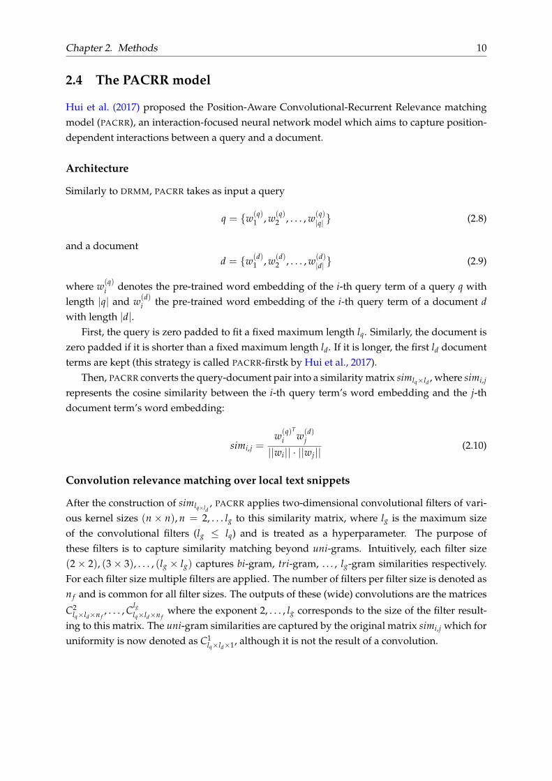
Pooling Layers
Subsequently, max pooling is applied to the n f dimension of each matrix
C2lq×ld×n f
. . . Clglq×ld×n f
to keep the strongest signal among those produced by the multiple (n f ) fil-
ters of a certain size. This process results to the matrices C2lq×ld×1 . . . Clg
lq×ld×1. At this point, each
row i of each matrix C1lq×ld×1, C2
lq×ld×1 . . . Clglq×ld×1 represents the relevance of the corresponding
(i-th) query term with the document at uni-gram, bi-gram, . . . , lg-gram level respectively. Asa second pooling strategy, k-max pooling is applied to each row of each matrix, keeping thestrongest k signals, resulting to the matrices P1
lq×k, . . . , Plglq×k. Finally, these matrices are concate-
nated on the k dimension to create the matrix Plq×(lg·k).
convolution row-wise k-max pooling
max pooling
DocumentQuery
...
...
concatenation
softmax
Query Terms’ IDF
...
...
Relevance Score
...
Concatenated Doc-Aware Query Term Encodings
DenseLayers
......
FIGURE 2.3: PACRR architecture.
IDF weighed representations
Now, each row i of matrix P1lq×(lg·k) is a document aware representation of the i-th query term.
The IDF scores of the query terms are also appended in the corresponding rows, after normal-izing them through softmax, in order to indicate the importance of each query term.
Document Scoring Layer
Since now every query term has a document aware representation vector, what is left is a layerto combine these representations into a single relevance score. This can be achieved by usingone of the following components:
Recurrent Layer: Each query term vector representation is passed through a Long-ShortTerm Memory (LSTM) recurrent layer (Hochreiter and Schmidhuber, 1997) with output dimen-sionality of one, in order to produce the final relevance score of the query-document pair. Thiswas the original version of PACRR proposed by Hui et al., 2017. We will refer to this variationof the model as PACRR-RNN.
Chapter 2. Methods 12
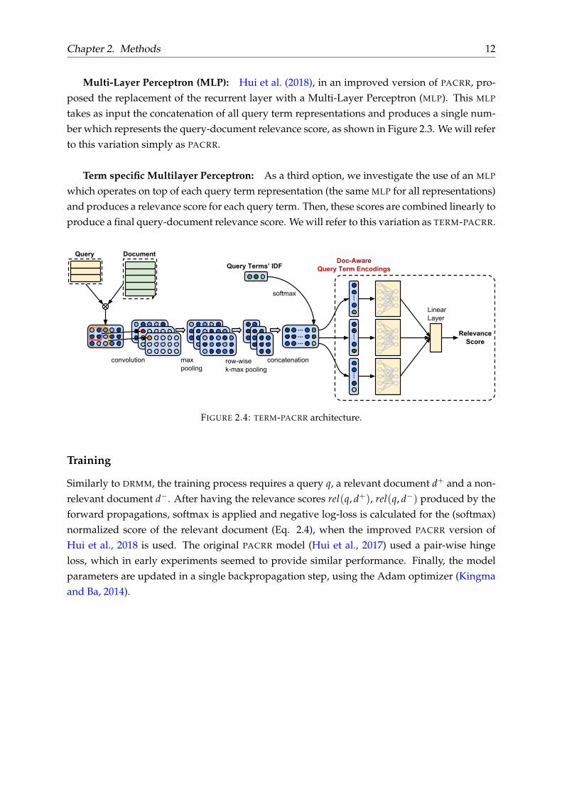
Multi-Layer Perceptron (MLP): Hui et al. (2018), in an improved version of PACRR, pro-posed the replacement of the recurrent layer with a Multi-Layer Perceptron (MLP). This MLP
takes as input the concatenation of all query term representations and produces a single num-ber which represents the query-document relevance score, as shown in Figure 2.3. We will referto this variation simply as PACRR.
Term specific Multilayer Perceptron: As a third option, we investigate the use of an MLP
which operates on top of each query term representation (the same MLP for all representations)and produces a relevance score for each query term. Then, these scores are combined linearly toproduce a final query-document relevance score. We will refer to this variation as TERM-PACRR.
convolution row-wise k-max pooling
max pooling
DocumentQuery
...
...
concatenation
softmax
Query Terms’ IDF
Relevance Score
LinearLayer
......
...
Doc-Aware Query Term Encodings
...
FIGURE 2.4: TERM-PACRR architecture.
Training
Similarly to DRMM, the training process requires a query q, a relevant document d+ and a non-relevant document d−. After having the relevance scores rel(q, d+), rel(q, d−) produced by theforward propagations, softmax is applied and negative log-loss is calculated for the (softmax)normalized score of the relevant document (Eq. 2.4), when the improved PACRR version ofHui et al., 2018 is used. The original PACRR model (Hui et al., 2017) used a pair-wise hingeloss, which in early experiments seemed to provide similar performance. Finally, the modelparameters are updated in a single backpropagation step, using the Adam optimizer (Kingmaand Ba, 2014).
Chapter 2. Methods 13
2.5 Extra features for exact match capturing
As an attempt to improve the reranking performance we will include the BM score of thedocument as an extra input to the deep relevance ranking models. Having a query q and a listof top N retrieved documents to be reranked, we normalize the BM scores of these documentsusing z-normalization as shown in Eq. 2.11, where µ, σ are the mean and standard deviation ofthe BM scores of the documents in the list respectively, si is the BM score of the i-th retrieveddocument and zi is the normalized score of this document which will be used as input to themodels.
zi =si − µ
σ(2.11)
Moreover, we will add three additional features that aim to provide strong signals of exactuni-gram or bi-gram matching between a query-document pair. Specifically, we will use threeoverlap features (Severyn and Moschitti, 2015; Mohan et al., 2017):
Uni-gram overlap (overlap1): Given the set of distinct tokens Uq for a query and the set ofdistinct tokens Ud for a document, uni-gram overlap is the number of common tokens betweenthe two sets, divided by the number of tokens in Uq (Eq. 2.12).
overlap1 =|Uq
⋂Ud|
|Uq|(2.12)
Bi-gram overlap (overlap2): Given the set of distinct bi-grams Bq for a query and the setof distinct bi-grams Bd for a document, bi-gram overlap is the number of common bi-gramsbetween the two sets, divided by the number of bi-grams in Bq (Eq. 2.13).
overlap2 =|Bq
⋂Bd|
|Bq|(2.13)
IDF weighted uni-gram overlap (overlap3): Given the set of distinct uni-grams Uq for aquery and the set of distinct bi-grams Ud for a document, IDF weighted uni-gram overlap is thesum of the IDF values of the common uni-grams between the two sets, divided by the sum ofthe IDF values of the uni-grams in Uq (Eq. 2.14).
overlap3 =∑t∈Uq
⋂Ud
IDF(t)
∑t∈UqIDF(t)
(2.14)
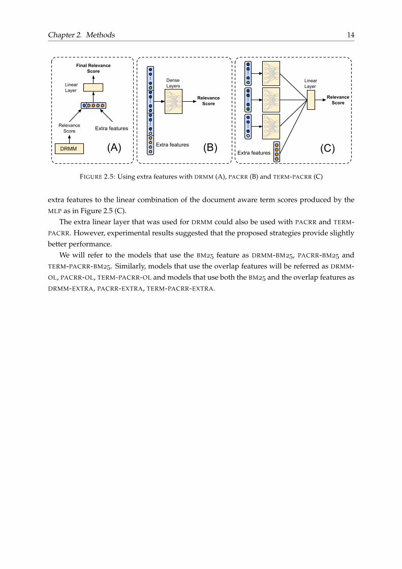
Using extra features with neural ranking models.
We will introduce the extra features to the DRMM model by linearly combining them with therelevance score produced by DRMM as visualized in Figure 2.5 (A).
For the PACRR model, we will append the extra features to the document aware concate-nated term representations as shown in Figure 2.5 (B). Then, extra features are passed to theMLP as part of this concatenated vector. Finally, for the TERM-PACRR model we will include the
Chapter 2. Methods 14
Relevance Score
LinearLayer
......
...
...
Relevance Score
... DenseLayers
......
Extra featuresExtra features
Relevance Score Extra features
Final Relevance Score
DRMM
LinearLayer
(A) (B) (C)
FIGURE 2.5: Using extra features with DRMM (A), PACRR (B) and TERM-PACRR (C)
extra features to the linear combination of the document aware term scores produced by theMLP as in Figure 2.5 (C).
The extra linear layer that was used for DRMM could also be used with PACRR and TERM-PACRR. However, experimental results suggested that the proposed strategies provide slightlybetter performance.
We will refer to the models that use the BM feature as DRMM-BM, PACRR-BM andTERM-PACRR-BM. Similarly, models that use the overlap features will be referred as DRMM-OL, PACRR-OL, TERM-PACRR-OL and models that use both the BM and the overlap features asDRMM-EXTRA, PACRR-EXTRA, TERM-PACRR-EXTRA.
15
Chapter 3
Experiments
3.1 Data
The main evaluation of the methods described in this work utilize data provided by the BIOASQ
challenge (Tsatsaronis et al., 2015). Methods are also evaluated on the TREC ROBUST 2004dataset (Voorhees, 2005) to confirm the consistency of the experimental results.
3.1.1 BioASQ dataset
The BioASQ challenge
BIOASQ is a biomedical semantic indexing and question answering (QA) challenge, which startedas a project funded by the European Union (2012-14)1, and is now supported by the U.S. Na-tional Library of Medicine of the National Institutes of Health2. The annual challenges, cur-rently in the 6th year (2018), include hierarchical text classification, information retrieval, QA
from texts and structured data as well as text summarization and other tasks.
The challenge is structured in two independent tasks3:
• Task A: Large-Scale Online Biomedical Semantic IndexingParticipants are asked to classify new PubMed abstracts into classes from the MeSH hier-archy4.
• Task B: Biomedical Semantic QA:This task includes IR, QA and summarization. Participants are given a training datasetcontaining biomedical questions with annotated answers and relevant information andare asked to respond to new test questions in two phases:
– phase A: Participants respond with relevant documents, snippets, concepts and RDFtriples from designated sources. In particular, at most 10 relevant documents shouldbe returned for each question, in decreasing order of relevance. At most 10 rele-vant snippets should be extracted from the 10 predicted relevant documents, also indecreasing order of relevance. This information is available during training.
1https://cordis.europa.eu/project/rcn/105774_en.html2https://www.nlm.nih.gov/3For more information on the tasks, see: http://bioasq.org/participate/challenges4See https://www.nlm.nih.gov/mesh/
Chapter 3. Experiments 16
– phase B: After the completion of phase A, gold relevant documents of the test queriesare made available for phase B and participants are asked to respond with exactanswers (e.g. named entities in the case of factoid questions) and ideal answers(paragrapsh-sized summaries).
A first evaluation of the participating systems is based of these gold documents. A sec-ond stage of manual evaluation (by biomedical experts) produces the final ranking of thesystems. During the manual evaluation, the experts add to the gold documents, snippets,answers etc. any system responses that were correct and were not originally included inthe gold ones.
Dateset description
For training and development of the models we will use the Task6b-phase A training data fromthe 6th BIOASQ challenge which contain 2251 English questions of biomedical interest and a listof documents for each question which are marked as relevant by biomedical experts, amongother annotated information (e.g. snippets) that are not directly relevant to this work.
The methods will then be used to predict relevant documents for the 500 queries (fivebatches of 100 queries) of the test data of the 6th year of BIOASQ. For their evaluation, the golddocuments of phase B will be used. We will refer to the BIOASQ test dataset as BIOASQ-TEST
and to a test batch B in particular as BIOASQTEST-BATCH-B.For the purposes of our experiments we further split the 2251 queries of the ’training’
dataset of the 6th year of BIOASQ into train and development sets so that the training set(BIOASQ-TRAIN) contains the 1751 queries corresponding to training queries created up tothe 5th year of BIOASQ and the development set (BIOASQ-DEV) contains the 500 queries addedto the ’training’ set for the 6th year, which were the test set of the 5th year (Figure 3.1). Table 3.1shows examples of BIOASQ queries.
BIOASQ queries1 In what proportion of children with heart failure has Enalapril been shown to be safe and effective?2 Which polyQ tract protein is linked to Spinocerebellar Ataxia type 2?3 What is the effect of amitriptyline in the mdx mouse model of Duchenne muscular dystrophy?4 What is the outcome of TAF10 interacting with the GATA1 transcription factor?5 Is there any association of the chromosomal region harboring the gene ITIH3 with schizophrenia?
TABLE 3.1: Examples of BIOASQ queries.
Dataset statistics
An important statistic for the document ranking task is the number of annotated (gold) relevantdocuments per query during training and development of the models for two reasons. First,the number of annotated relevant documents is proportional to the number of the extractedtraining examples, so more annotated relevant documents will most probably result to moretraining examples. An other reason is that a small number of annotated documents could lead
Chapter 3. Experiments 17
bioasq-train
77.8%
bioasq-dev
22.2%
FIGURE 3.1: Percentage of BIOASQ-TRAIN and BIOASQ-DEV sets over the whole’training’ dataset provided by the BIOASQ phase A challenge.
to low performance scores on the development set due to retrieving (or ranking high) relevantdocuments that were not annotated by humans.
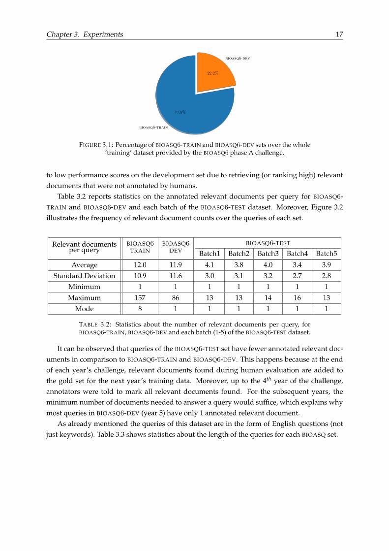
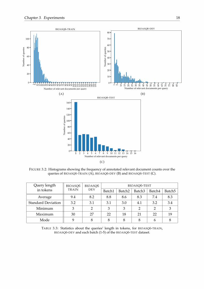
Table 3.2 reports statistics on the annotated relevant documents per query for BIOASQ-TRAIN and BIOASQ-DEV and each batch of the BIOASQ-TEST dataset. Moreover, Figure 3.2illustrates the frequency of relevant document counts over the queries of each set.
Relevant documentsper query
BIOASQTRAIN
BIOASQDEV
BIOASQ-TEST
Batch1 Batch2 Batch3 Batch4 Batch5
Average 12.0 11.9 4.1 3.8 4.0 3.4 3.9
Standard Deviation 10.9 11.6 3.0 3.1 3.2 2.7 2.8
Minimum 1 1 1 1 1 1 1
Maximum 157 86 13 13 14 16 13
Mode 8 1 1 1 1 1 1
TABLE 3.2: Statistics about the number of relevant documents per query, forBIOASQ-TRAIN, BIOASQ-DEV and each batch (1-5) of the BIOASQ-TEST dataset.
It can be observed that queries of the BIOASQ-TEST set have fewer annotated relevant doc-uments in comparison to BIOASQ-TRAIN and BIOASQ-DEV. This happens because at the endof each year’s challenge, relevant documents found during human evaluation are added tothe gold set for the next year’s training data. Moreover, up to the 4th year of the challenge,annotators were told to mark all relevant documents found. For the subsequent years, theminimum number of documents needed to answer a query would suffice, which explains whymost queries in BIOASQ-DEV (year 5) have only 1 annotated relevant document.
As already mentioned the queries of this dataset are in the form of English questions (notjust keywords). Table 3.3 shows statistics about the length of the queries for each BIOASQ set.
Chapter 3. Experiments 18
1 5 10 15 20 25 30 35 40 45 50 55 60 65 70 75 80 85 90 95 100
105
110
115
120
125
130
135
140
145
150
155
Number of relevant documents per query
0
20
40
60
80
100
Num
ber
ofqu
erie
s
BIOASQ6-TRAIN
(A)
1 5 10 15 20 25 30 35 40 45 50 55 60 65 70 75 80 85
Number of relevant documents per query
0
10
20
30
40
50
60
70
80
Num
ber
ofqu
erie
s
BIOASQ6-DEV
(B)
11 2 3 4 5 6 7 8 9 10 11 12 13 14 15 16Number of relevant documents per query
0
20
40
60
80
100
120
140
160
Num
ber
ofqu
erie
s
BIOASQ6-TEST
(C)
FIGURE 3.2: Histograms showing the frequency of annotated relevant document counts over thequeries of BIOASQ-TRAIN (A), BIOASQ-DEV (B) and BIOASQ-TEST (C).
Query lengthin tokens
BIOASQTRAIN
BIOASQDEV
BIOASQ-TEST
Batch1 Batch2 Batch3 Batch4 Batch5
Average 9.4 8.2 8.8 8.6 8.3 7.4 8.3
Standard Deviation 3.2 3.1 3.1 3.0 4.1 3.2 3.4
Minimum 3 2 3 3 2 2 3
Maximum 30 27 22 18 21 22 19
Mode 9 8 8 8 8 6 8
TABLE 3.3: Statistics about the queries’ length in tokens, for BIOASQ-TRAIN,BIOASQ-DEV and each batch (1-5) of the BIOASQ-TEST dataset.
Chapter 3. Experiments 19
Document Collection
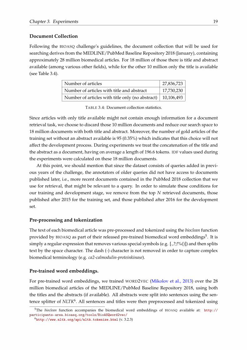
Following the BIOASQ challenge’s guidelines, the document collection that will be used forsearching derives from the MEDLINE/PubMed Baseline Repository 2018 (January), containingapproximately 28 million biomedical articles. For 18 million of those there is title and abstractavailable (among various other fields), while for the other 10 million only the title is available(see Table 3.4).
Number of articles 27,836,723
Number of articles with title and abstract 17,730,230
Number of articles with title only (no abstract) 10,106,493
TABLE 3.4: Document collection statistics.
Since articles with only title available might not contain enough information for a documentretrieval task, we choose to discard those 10 million documents and reduce our search space to18 million documents with both title and abstract. Moreover, the number of gold articles of thetraining set without an abstract available is 95 (0.35%) which indicates that this choice will notaffect the development process. During experiments we treat the concatenation of the title andthe abstract as a document, having on average a length of 196.6 tokens. IDF values used duringthe experiments were calculated on these 18 million documents.
At this point, we should mention that since the dataset consists of queries added in previ-ous years of the challenge, the annotators of older queries did not have access to documentspublished later, i.e., more recent documents contained in the PubMed 2018 collection that weuse for retrieval, that might be relevant to a query. In order to simulate these conditions forour training and development stage, we remove from the top N retrieved documents, thosepublished after 2015 for the training set, and those published after 2016 for the developmentset.
Pre-processing and tokenization
The text of each biomedical article was pre-processed and tokenized using the bioclean functionprovided by BIOASQ as part of their released pre-trained biomedical word embeddings5. It issimply a regular expression that removes various special symbols (e.g. [.,?;!%()]) and then splitstext by the space character. The dash (-) character is not removed in order to capture complexbiomedical terminology (e.g. ca2-calmodulin-proteinkinase).
Pre-trained word embeddings.
For pre-trained word embeddings, we trained WORD2VEC (Mikolov et al., 2013) over the 28million biomedical articles of the MEDLINE/PubMed Baseline Repository 2018, using boththe titles and the abstracts (if available). All abstracts were split into sentences using the sen-tence splitter of NLTK6. All sentences and titles were then preprocessed and tokenized using
5The bioclean function accompanies the biomedical word embeddings of BIOASQ available at: http://participants-area.bioasq.org/tools/BioASQword2vec/
6http://www.nltk.org/api/nltk.tokenize.html (v. 3.2.3)
Chapter 3. Experiments 20
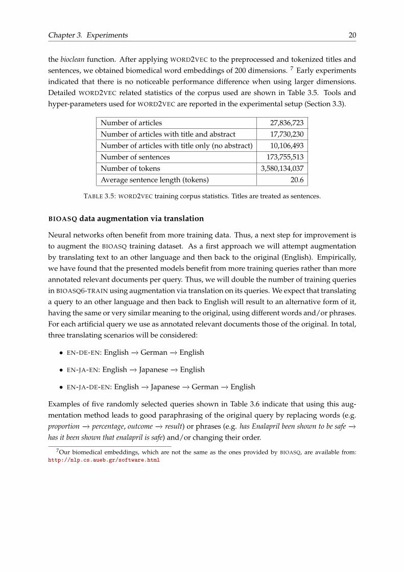
the bioclean function. After applying WORD2VEC to the preprocessed and tokenized titles andsentences, we obtained biomedical word embeddings of 200 dimensions. 7 Early experimentsindicated that there is no noticeable performance difference when using larger dimensions.Detailed WORD2VEC related statistics of the corpus used are shown in Table 3.5. Tools andhyper-parameters used for WORD2VEC are reported in the experimental setup (Section 3.3).
Number of articles 27,836,723
Number of articles with title and abstract 17,730,230
Number of articles with title only (no abstract) 10,106,493
Number of sentences 173,755,513
Number of tokens 3,580,134,037
Average sentence length (tokens) 20.6
TABLE 3.5: WORD2VEC training corpus statistics. Titles are treated as sentences.
BIOASQ data augmentation via translation
Neural networks often benefit from more training data. Thus, a next step for improvement isto augment the BIOASQ training dataset. As a first approach we will attempt augmentationby translating text to an other language and then back to the original (English). Empirically,we have found that the presented models benefit from more training queries rather than moreannotated relevant documents per query. Thus, we will double the number of training queriesin BIOASQ-TRAIN using augmentation via translation on its queries. We expect that translatinga query to an other language and then back to English will result to an alternative form of it,having the same or very similar meaning to the original, using different words and/or phrases.For each artificial query we use as annotated relevant documents those of the original. In total,three translating scenarios will be considered:
• EN-DE-EN: English −→ German −→ English
• EN-JA-EN: English −→ Japanese −→ English
• EN-JA-DE-EN: English −→ Japanese −→ German −→ English
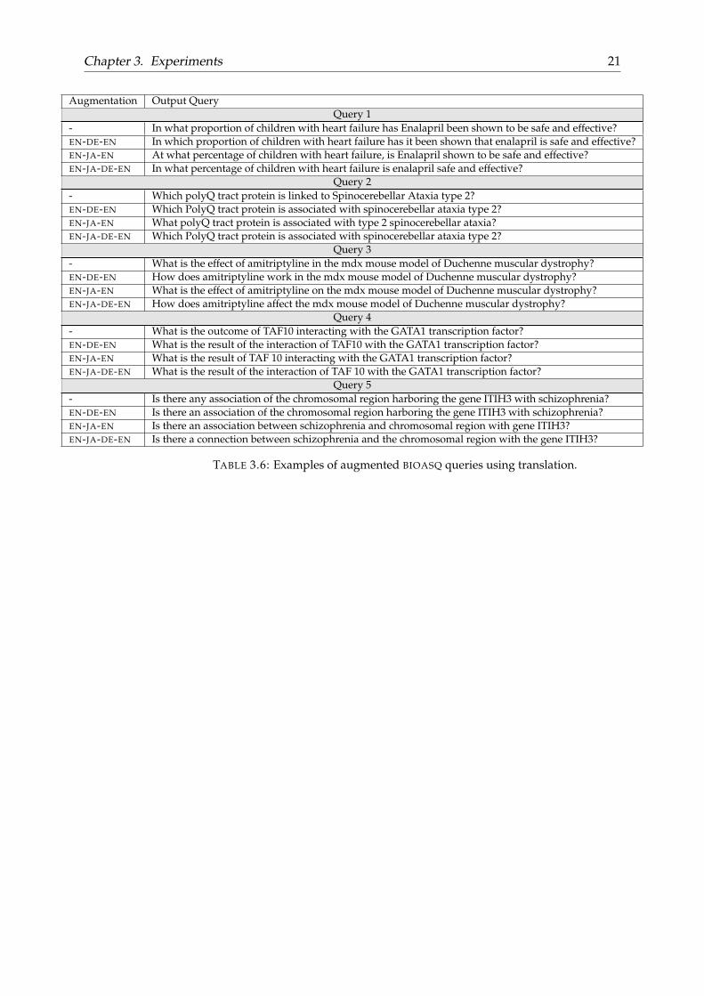
Examples of five randomly selected queries shown in Table 3.6 indicate that using this aug-mentation method leads to good paraphrasing of the original query by replacing words (e.g.proportion −→ percentage, outcome −→ result) or phrases (e.g. has Enalapril been shown to be safe −→has it been shown that enalapril is safe) and/or changing their order.
7Our biomedical embeddings, which are not the same as the ones provided by BIOASQ, are available from:http://nlp.cs.aueb.gr/software.html
Chapter 3. Experiments 21
Augmentation Output QueryQuery 1
- In what proportion of children with heart failure has Enalapril been shown to be safe and effective?EN-DE-EN In which proportion of children with heart failure has it been shown that enalapril is safe and effective?EN-JA-EN At what percentage of children with heart failure, is Enalapril shown to be safe and effective?EN-JA-DE-EN In what percentage of children with heart failure is enalapril safe and effective?
Query 2- Which polyQ tract protein is linked to Spinocerebellar Ataxia type 2?EN-DE-EN Which PolyQ tract protein is associated with spinocerebellar ataxia type 2?EN-JA-EN What polyQ tract protein is associated with type 2 spinocerebellar ataxia?EN-JA-DE-EN Which PolyQ tract protein is associated with spinocerebellar ataxia type 2?
Query 3- What is the effect of amitriptyline in the mdx mouse model of Duchenne muscular dystrophy?EN-DE-EN How does amitriptyline work in the mdx mouse model of Duchenne muscular dystrophy?EN-JA-EN What is the effect of amitriptyline on the mdx mouse model of Duchenne muscular dystrophy?EN-JA-DE-EN How does amitriptyline affect the mdx mouse model of Duchenne muscular dystrophy?
Query 4- What is the outcome of TAF10 interacting with the GATA1 transcription factor?EN-DE-EN What is the result of the interaction of TAF10 with the GATA1 transcription factor?EN-JA-EN What is the result of TAF 10 interacting with the GATA1 transcription factor?EN-JA-DE-EN What is the result of the interaction of TAF 10 with the GATA1 transcription factor?
Query 5- Is there any association of the chromosomal region harboring the gene ITIH3 with schizophrenia?EN-DE-EN Is there an association of the chromosomal region harboring the gene ITIH3 with schizophrenia?EN-JA-EN Is there an association between schizophrenia and chromosomal region with gene ITIH3?EN-JA-DE-EN Is there a connection between schizophrenia and the chromosomal region with the gene ITIH3?
TABLE 3.6: Examples of augmented BIOASQ queries using translation.
Chapter 3. Experiments 22
3.1.2 TREC Robust2004 dataset
The second dataset that we will use is the TREC ROBUST 2004 dataset (Voorhees, 2005) whichis widely used to evaluate conventional ad-hoc retrieval systems and recent neural models likeDRMM (Guo et al., 2016).
Dataset description
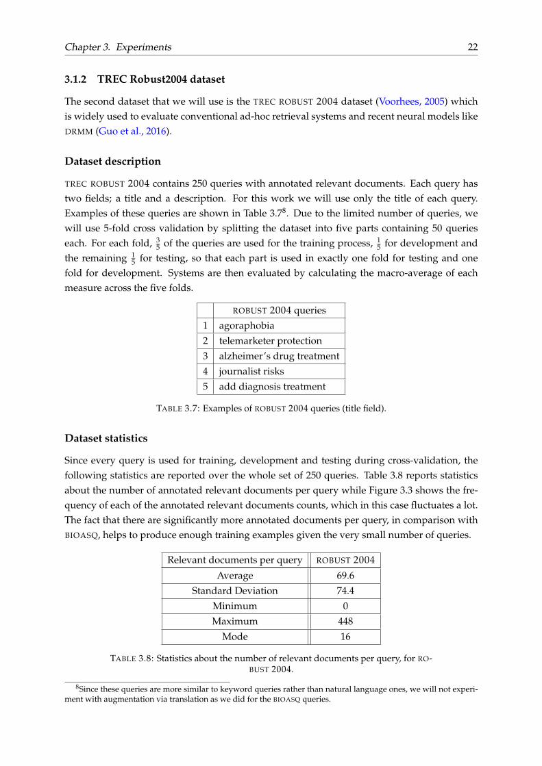
TREC ROBUST 2004 contains 250 queries with annotated relevant documents. Each query hastwo fields; a title and a description. For this work we will use only the title of each query.Examples of these queries are shown in Table 3.78. Due to the limited number of queries, wewill use 5-fold cross validation by splitting the dataset into five parts containing 50 querieseach. For each fold, 3
5 of the queries are used for the training process, 15 for development and
the remaining 15 for testing, so that each part is used in exactly one fold for testing and one
fold for development. Systems are then evaluated by calculating the macro-average of eachmeasure across the five folds.
ROBUST 2004 queries
1 agoraphobia
2 telemarketer protection
3 alzheimer’s drug treatment
4 journalist risks
5 add diagnosis treatment
TABLE 3.7: Examples of ROBUST 2004 queries (title field).
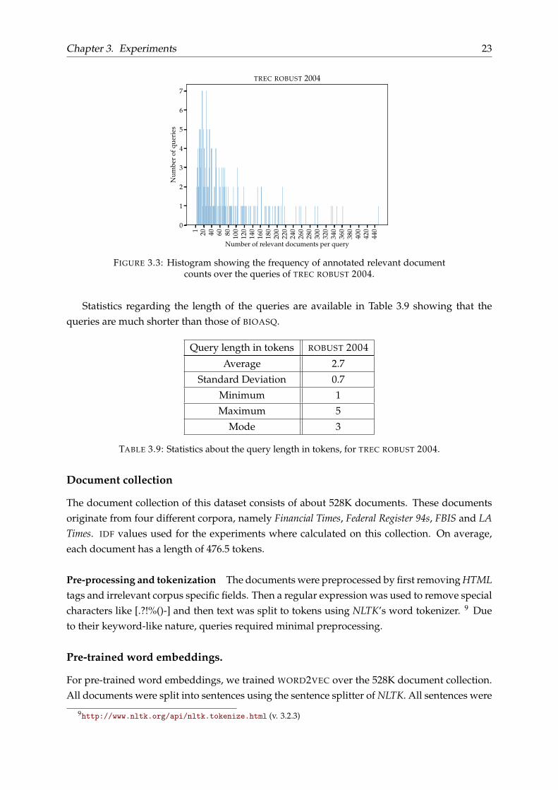
Dataset statistics
Since every query is used for training, development and testing during cross-validation, thefollowing statistics are reported over the whole set of 250 queries. Table 3.8 reports statisticsabout the number of annotated relevant documents per query while Figure 3.3 shows the fre-quency of each of the annotated relevant documents counts, which in this case fluctuates a lot.The fact that there are significantly more annotated documents per query, in comparison withBIOASQ, helps to produce enough training examples given the very small number of queries.
Relevant documents per query ROBUST 2004
Average 69.6
Standard Deviation 74.4
Minimum 0
Maximum 448
Mode 16
TABLE 3.8: Statistics about the number of relevant documents per query, for RO-BUST 2004.
8Since these queries are more similar to keyword queries rather than natural language ones, we will not experi-ment with augmentation via translation as we did for the BIOASQ queries.
Chapter 3. Experiments 23
1 20 40 60 80 100
120
140
160
180
200
220
240
260
280
300
320
340
360
380
400
420
440
Number of relevant documents per query
0
1
2
3
4
5
6
7
Num
ber
ofqu
erie
s
TREC ROBUST 2004
FIGURE 3.3: Histogram showing the frequency of annotated relevant documentcounts over the queries of TREC ROBUST 2004.
Statistics regarding the length of the queries are available in Table 3.9 showing that thequeries are much shorter than those of BIOASQ.
Query length in tokens ROBUST 2004
Average 2.7
Standard Deviation 0.7
Minimum 1
Maximum 5
Mode 3
TABLE 3.9: Statistics about the query length in tokens, for TREC ROBUST 2004.
Document collection
The document collection of this dataset consists of about 528K documents. These documentsoriginate from four different corpora, namely Financial Times, Federal Register 94s, FBIS and LATimes. IDF values used for the experiments where calculated on this collection. On average,each document has a length of 476.5 tokens.
Pre-processing and tokenization The documents were preprocessed by first removing HTMLtags and irrelevant corpus specific fields. Then a regular expression was used to remove specialcharacters like [.?!%()-] and then text was split to tokens using NLTK’s word tokenizer. 9 Dueto their keyword-like nature, queries required minimal preprocessing.
Pre-trained word embeddings.
For pre-trained word embeddings, we trained WORD2VEC over the 528K document collection.All documents were split into sentences using the sentence splitter of NLTK. All sentences were
9http://www.nltk.org/api/nltk.tokenize.html (v. 3.2.3)
Chapter 3. Experiments 24
then preprocessed and tokenized. After applying WORD2VEC to the preprocessed and tok-enized sentences, we obtained word embeddings of 200 dimensions (see Section 3.3).
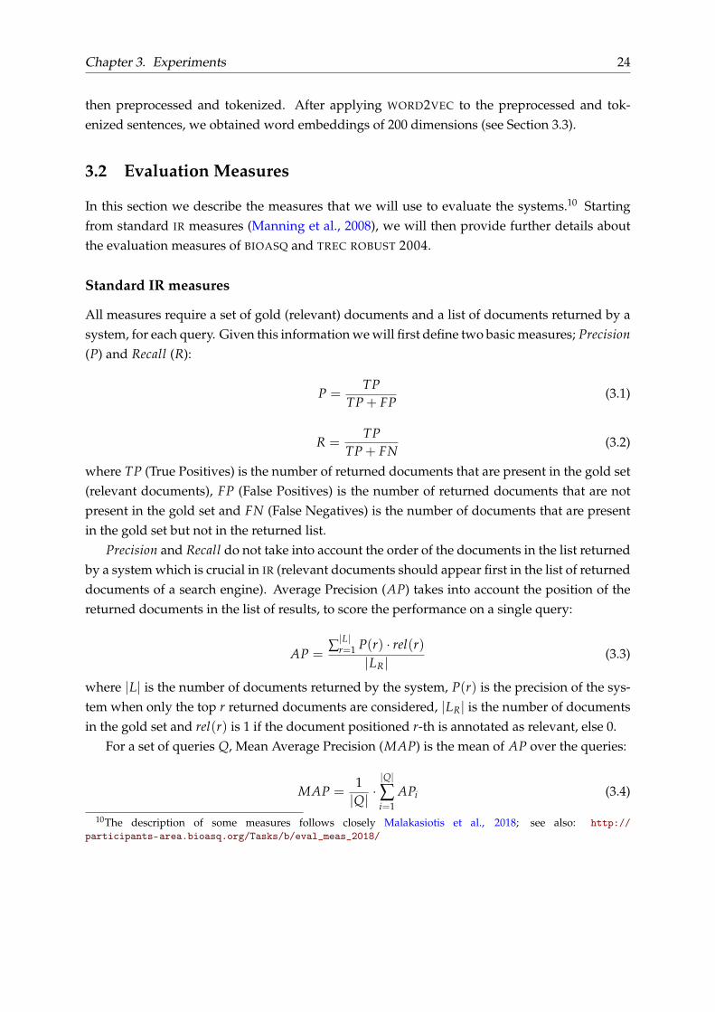
3.2 Evaluation Measures
In this section we describe the measures that we will use to evaluate the systems.10 Startingfrom standard IR measures (Manning et al., 2008), we will then provide further details aboutthe evaluation measures of BIOASQ and TREC ROBUST 2004.
Standard IR measures
All measures require a set of gold (relevant) documents and a list of documents returned by asystem, for each query. Given this information we will first define two basic measures; Precision(P) and Recall (R):
P =TP
TP + FP(3.1)
R =TP
TP + FN(3.2)
where TP (True Positives) is the number of returned documents that are present in the gold set(relevant documents), FP (False Positives) is the number of returned documents that are notpresent in the gold set and FN (False Negatives) is the number of documents that are presentin the gold set but not in the returned list.
Precision and Recall do not take into account the order of the documents in the list returnedby a system which is crucial in IR (relevant documents should appear first in the list of returneddocuments of a search engine). Average Precision (AP) takes into account the position of thereturned documents in the list of results, to score the performance on a single query:
AP =∑|L|r=1 P(r) · rel(r)
|LR|(3.3)
where |L| is the number of documents returned by the system, P(r) is the precision of the sys-tem when only the top r returned documents are considered, |LR| is the number of documentsin the gold set and rel(r) is 1 if the document positioned r-th is annotated as relevant, else 0.
For a set of queries Q, Mean Average Precision (MAP) is the mean of AP over the queries:
MAP =1|Q| ·
|Q|
∑i=1
APi (3.4)
10The description of some measures follows closely Malakasiotis et al., 2018; see also: http://participants-area.bioasq.org/Tasks/b/eval_meas_2018/
Chapter 3. Experiments 25
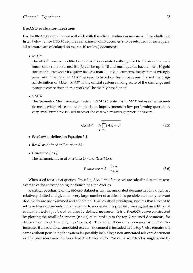
BioASQ evaluation measures
For the BIOASQ evaluation we will stick with the official evaluation measures of the challenge,listed below. Since BIOASQ requires a maximum of 10 documents to be returned for each query,all measures are calculated on the top 10 (or less) documents:
• MAP?
The MAP measure modified so that AP is calculated with LR fixed to 10, since the max-imum size of the returned list |L| can be up to 10 and most queries have at least 10 golddocuments. However if a query has less than 10 gold documents, the system is wronglypenalized. The notation MAP? is used to avoid confusion between this and the origi-nal definition of MAP. MAP? is the official system ranking score of the challenge andsystems’ comparison in this work will be mainly based on it.
• GMAPThe Geometric Mean Average Precision (GMAP) is similar to MAP but uses the geomet-ric mean which places more emphasis on improvements in low performing queries. Avery small number ε is used to cover the case where average precision is zero.
GMAP = n
√n
∏i=1
(APi + ε) (3.5)
• Precision as defined in Equation 3.1.
• Recall as defined in Equation 3.2.
• F-measure (or F1)The harmonic mean of Precision (P) and Recall (R):
F-measure = 2 · P · RP + R
(3.6)
When used for a set of queries, Precision, Recall and F-measure are calculated as the macro-average of the corresponding measure along the queries.
A critical peculiarity of the BIOASQ dataset is that the annotated documents for a query arerelatively limited and given the very large number of articles, it is possible that many relevantdocuments are not examined and annotated. This results to penalizing systems that succeed toretrieve these documents. In an attempt to moderate this problem, we suggest an additionalevaluation technique based on already defined measures. It is a Recall@k curve constructedby plotting the recall of a system (y-axis) calculated up to the top k returned documents, fordifferent values of k = 1, 2, . . . , N (x-axis). This way, whenever k increases by 1, Recall@kincreases if an additional annotated relevant document is included in the top k, else remains thesame without penalizing the system for possibly including a non-annotated relevant documentas any precision based measure like MAP would do. We can also extract a single score by
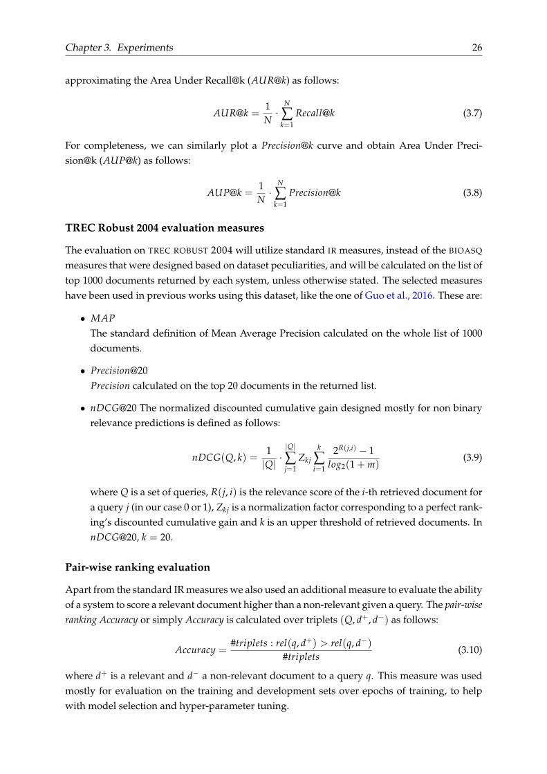
Chapter 3. Experiments 26
approximating the Area Under Recall@k (AUR@k) as follows:
AUR@k =1N·
N
∑k=1
Recall@k (3.7)
For completeness, we can similarly plot a Precision@k curve and obtain Area Under Preci-sion@k (AUP@k) as follows:
AUP@k =1N·
N
∑k=1
Precision@k (3.8)
TREC Robust 2004 evaluation measures
The evaluation on TREC ROBUST 2004 will utilize standard IR measures, instead of the BIOASQ
measures that were designed based on dataset peculiarities, and will be calculated on the list oftop 1000 documents returned by each system, unless otherwise stated. The selected measureshave been used in previous works using this dataset, like the one of Guo et al., 2016. These are:
• MAPThe standard definition of Mean Average Precision calculated on the whole list of 1000documents.
• Precision@20Precision calculated on the top 20 documents in the returned list.
• nDCG@20 The normalized discounted cumulative gain designed mostly for non binaryrelevance predictions is defined as follows:
nDCG(Q, k) =1|Q| ·
|Q|
∑j=1
Zkj
k
∑i=1
2R(j,i) − 1log2(1 + m)
(3.9)
where Q is a set of queries, R(j, i) is the relevance score of the i-th retrieved document fora query j (in our case 0 or 1), Zkj is a normalization factor corresponding to a perfect rank-ing’s discounted cumulative gain and k is an upper threshold of retrieved documents. InnDCG@20, k = 20.
Pair-wise ranking evaluation
Apart from the standard IR measures we also used an additional measure to evaluate the abilityof a system to score a relevant document higher than a non-relevant given a query. The pair-wiseranking Accuracy or simply Accuracy is calculated over triplets (Q, d+, d−) as follows:
Accuracy =#triplets : rel(q, d+) > rel(q, d−)
#triplets(3.10)
where d+ is a relevant and d− a non-relevant document to a query q. This measure was usedmostly for evaluation on the training and development sets over epochs of training, to helpwith model selection and hyper-parameter tuning.
Chapter 3. Experiments 27
3.3 Experimental Setup
3.3.1 Initial document retrieval
The first step of the experimental pipeline is to retrieve N documents for each query. For thispurpose, we used the Galago11 search engine with its scoring function set to BM, a relativelysimple but powerful method described in Chapter 2.
During indexing, stemming was applied to the documents and queries respectively, usingthe Krovetz stemmer (Krovetz, 1993). All documents were preprocessed using the dedicatedpreprocessing of each dataset. Specifically for BIOASQ the bioclean function was modified sothat text is also split on dashes (-) which proved useful at least for the BM retrieval mostlybecause it provided higher recall, a measure essential to reranking. During searching, querieswere preprocessed and stop-words were removed based on a dedicated list of stop-words foreach dataset. This retrieval setup will be referred as BM-SE.
3.3.2 Document reranking with neural networks
Training examples In order to use a dataset to train a neural network model, we will generatetraining pairs of a relevant and a non-relevant document for a query. For a query q let Drel bethe set of documents marked as relevant by humans. First, we retrieve the top N documentsusing BM-SE which constitute a set of documents Dret. Let DrelRet be the set of retrieveddocuments that are annotated as relevant:
DrelRet = Drel ∩ Dret (3.11)
Similarly, let DnonRelRet be the set of retrieved documents that are not marked as relevant:
DnonRelRet = Dret − Drel (3.12)
For each document d+ in DrelRet we randomly sample a document d− from DnonrelRet andthen produce a training example (q, d+, d−), i.e. a query, a relevant document and a non-relevant document. The number of training examples produced by this query q will be equal tothe size of DrelRet set. After repeating this process for every query in the training set, we obtainall the examples that we will use for the training of the neural networks. Early experimentsindicated that using relevant documents not returned in the top N documents as positive doc-uments to produce more training examples, leads to worse results. Moreover, using only theretrieved relevant documents makes it straightforward to use the BM score already calculatedby BM-SE, as input to the deep relevance matching models.
The number of documents retrieved with BM-SE and used for training and re-ranking wasset to N = 100 for the BIOASQ dataset and N = 1000 for the ROBUST 2004 dataset, numbers thatprovided a lot of room for reranking improvement (see Section 3.4) while keeping the numberof documents to score low. Table 3.10 shows the number of training examples produced afterthe process described above, using the top N documents, as defined above for each dataset.
11The Galago search engine: https://www.lemurproject.org/galago.php (v. 3.10)
Chapter 3. Experiments 28
Dataset #Training examples
BIOASQ 11, 590
+EN-DE-EN 22, 282
+EN-JA-EN 20, 554
+EN-JA-DE-EN 20, 148
ROBUST 2004 5, 934± 201
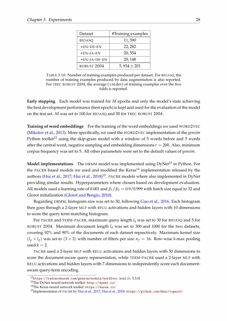
TABLE 3.10: Number of training examples produced per dataset. For BIOASQ, thenumber of training examples produced by data augmentation is also reported.For TREC ROBUST 2004, the average (±st.dev) of training examples over the five
folds is reported.
Early stopping Each model was trained for M epochs and only the model’s state achievingthe best development performance (best epoch) is kept and used for the evaluation of the modelon the test set. M was set to 100 for BIOASQ and 50 for TREC ROBUST 2004.
Training of word embeddings For the training of the word embeddings we used WORD2VEC
(Mikolov et al., 2013). More specifically, we used the WORD2VEC implementation of the gensimPython toolkit12 using the skip-gram model with a window of 5 words before and 5 wordsafter the central word, negative sampling and embedding dimensions r = 200. Also, minimumcorpus frequency was set to 5. All other parameters were set to the default values of gensim.
Model implementations The DRMM model was implemented using DyNet13 in Python. Forthe PACRR based models we used and modified the Keras14 implementation released by theauthors (Hui et al., 2017; Hui et al., 2018)15. PACRR models where also implemented in DyNetproviding similar results. Hyperparameters where chosen based on development evaluation.All models used a learning rate of 0.001 and β1/β2 = 0.9/0.999 with batch size equal to 32 andGlorot initialization (Glorot and Bengio, 2010).
Regarding DRMM, histogram size was set to 30, following Guo et al., 2016. Each histogramthen goes through a 2-layer MLP with RELU activations and hidden layers with 10 dimensionsto score the query term matching histogram.
For PACRR and TERM-PACRR, maximum query length lq was set to 30 for BIOASQ and 5 forROBUST 2004. Maximum document length ld was set to 300 and 1000 for the two datasets,covering 92% and 90% of the documents of each dataset repsectively. Maximum kernel size(lg × lg) was set to (3× 3) with number of filters per size n f = 16. Row-wise k-max poolingused k = 2.
PACRR used a 2-layer MLP with RELU activations and hidden layers with 50 dimensions toscore the document-aware query representation, while TERM-PACRR used a 2-layer MLP withRELU activations and hidden layers with 7 dimensions to independently score each document-aware query-term encoding.
12https://radimrehurek.com/gensim/models/word2vec.html (v. 3.3.0)13The DyNet neural network toolkit: http://dynet.io/14The Keras neural network toolkit: https://keras.io/15Implementation of PACRR by Hui et al., 2017; Hui et al., 2018: https://github.com/khui/copacrr

Chapter 3. Experiments 29
Evaluation The BIOASQ measures were calculated using BIOASQ’s official evaluation script16
and the TREC ROBUST 2004 measures using the trec_eval tool17.
3.4 Ideal reranking
As oracle we will refer to a reranking system that can always place the relevant documentson the top positions of the retrieved list of documents by having access to the relevance judg-ments of each query. Similarly to the neural re-ranking methods, we will apply oracle to thelist of documents retrieved by BM-SE, in order to find out the best possible performance thata reranking system can achieve (ideal reranking). It is easily perceived that the oracle’s perfor-mance is strongly associated with the number of relevant documents found in the retrieved list,that is the recall of BM-SE.
3.5 Experimental results
This section presents the experimental results of the systems described, on BIOASQ and TREC
ROBUST 2004 datasets. All reported results are the average of five different runs (five randominitializations) with standard deviation shown for each model (unless otherwise stated).
3.5.1 BioASQ experiments
First we are going to evaluate the methods on BIOASQ-DEV and then on BIOASQ-TEST toexamine the consistency of each system’s performance. Finally, we present the results of ourparticipation in the document retrieval task of the 6th year of BIOASQ (Task6b-phase A) thattook place during March to May 2018.
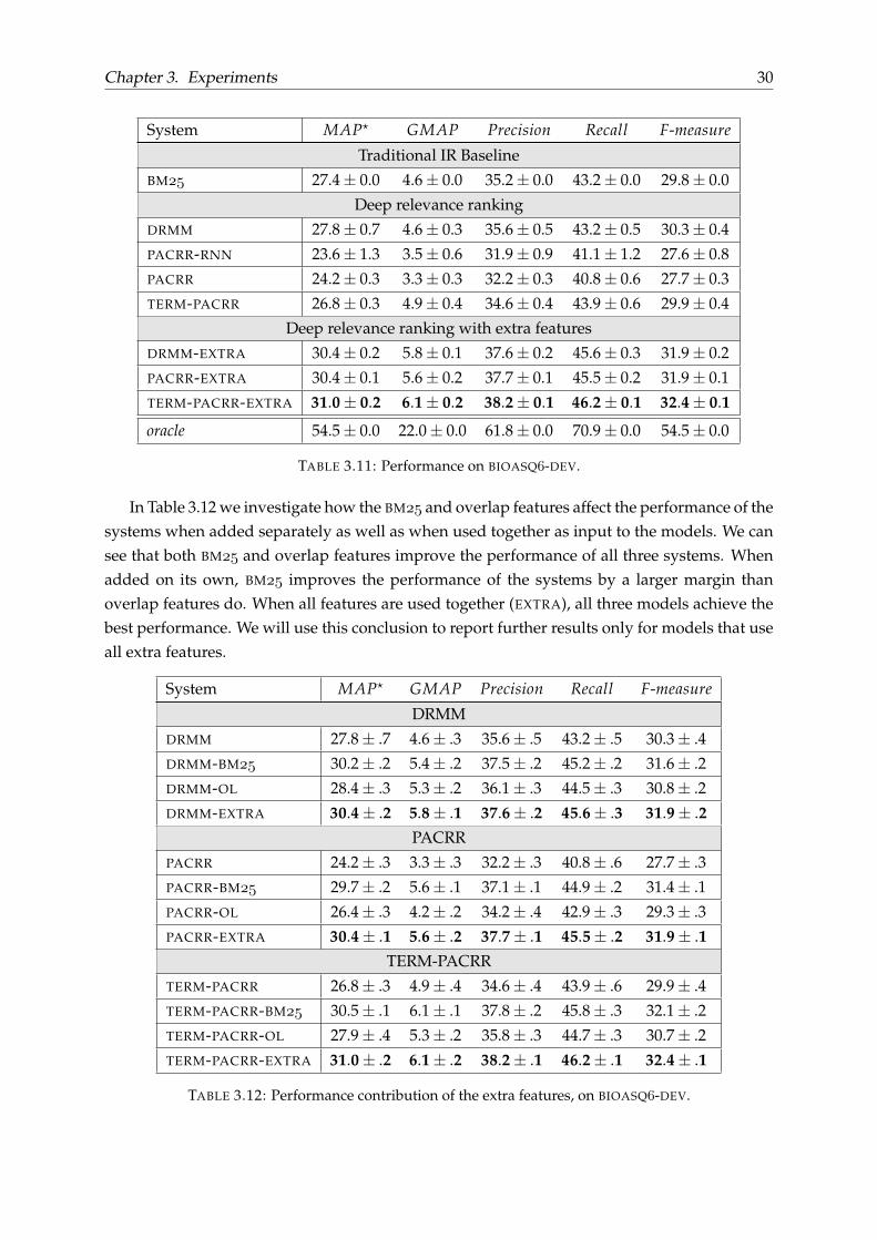
Table 3.11 reports the performance of the methods in the BIOASQ-DEV set. System rankingis based on MAP?. We can see that BM outperforms both PACRR and TERM-PACRR modelswith the latter performing significantly better than the former. Also, PACRR-RNN performsworse and is less consistent than its revised model, PACRR. DRMM performs slightly better thanBM and outperforms the other PACRR based methods, when external features are not used.After the addition of the BM and overlap features to the deep relevance ranking models, allthree models are significantly improved and outperform BM by a larger margin. Among thethree models using the extra features, TERM-PACRR-EXTRA is the best performing model onBIOASQ-DEV data. Finally, we can observe that the oracle’s performance is quite high whichindicates the reranking performance is not capped and can be improved further.
16The oficcial evaluation script of BIOASQ: https://github.com/BioASQ/Evaluation-Measures17The trec_eval tool for ad-hoc IR evaluation: https://trec.nist.gov/trec_eval/ (v. 9.0)
Chapter 3. Experiments 30
System MAP? GMAP Precision Recall F-measure
Traditional IR Baseline
BM 27.4± 0.0 4.6± 0.0 35.2± 0.0 43.2± 0.0 29.8± 0.0
Deep relevance ranking
DRMM 27.8± 0.7 4.6± 0.3 35.6± 0.5 43.2± 0.5 30.3± 0.4
PACRR-RNN 23.6± 1.3 3.5± 0.6 31.9± 0.9 41.1± 1.2 27.6± 0.8
PACRR 24.2± 0.3 3.3± 0.3 32.2± 0.3 40.8± 0.6 27.7± 0.3
TERM-PACRR 26.8± 0.3 4.9± 0.4 34.6± 0.4 43.9± 0.6 29.9± 0.4
Deep relevance ranking with extra features
DRMM-EXTRA 30.4± 0.2 5.8± 0.1 37.6± 0.2 45.6± 0.3 31.9± 0.2
PACRR-EXTRA 30.4± 0.1 5.6± 0.2 37.7± 0.1 45.5± 0.2 31.9± 0.1
TERM-PACRR-EXTRA 31.0± 0.2 6.1± 0.2 38.2± 0.1 46.2± 0.1 32.4± 0.1
oracle 54.5± 0.0 22.0± 0.0 61.8± 0.0 70.9± 0.0 54.5± 0.0
TABLE 3.11: Performance on BIOASQ-DEV.
In Table 3.12 we investigate how the BM and overlap features affect the performance of thesystems when added separately as well as when used together as input to the models. We cansee that both BM and overlap features improve the performance of all three systems. Whenadded on its own, BM improves the performance of the systems by a larger margin thanoverlap features do. When all features are used together (EXTRA), all three models achieve thebest performance. We will use this conclusion to report further results only for models that useall extra features.
System MAP? GMAP Precision Recall F-measure
DRMM
DRMM 27.8± .7 4.6± .3 35.6± .5 43.2± .5 30.3± .4
DRMM-BM 30.2± .2 5.4± .2 37.5± .2 45.2± .2 31.6± .2
DRMM-OL 28.4± .3 5.3± .2 36.1± .3 44.5± .3 30.8± .2
DRMM-EXTRA 30.4± .2 5.8± .1 37.6± .2 45.6± .3 31.9± .2PACRR
PACRR 24.2± .3 3.3± .3 32.2± .3 40.8± .6 27.7± .3
PACRR-BM 29.7± .2 5.6± .1 37.1± .1 44.9± .2 31.4± .1
PACRR-OL 26.4± .3 4.2± .2 34.2± .4 42.9± .3 29.3± .3
PACRR-EXTRA 30.4± .1 5.6± .2 37.7± .1 45.5± .2 31.9± .1TERM-PACRR
TERM-PACRR 26.8± .3 4.9± .4 34.6± .4 43.9± .6 29.9± .4
TERM-PACRR-BM 30.5± .1 6.1± .1 37.8± .2 45.8± .3 32.1± .2
TERM-PACRR-OL 27.9± .4 5.3± .2 35.8± .3 44.7± .3 30.7± .2
TERM-PACRR-EXTRA 31.0± .2 6.1± .2 38.2± .1 46.2± .1 32.4± .1
TABLE 3.12: Performance contribution of the extra features, on BIOASQ-DEV.
Chapter 3. Experiments 31
2 4 6 8 10top-k documents
0.2
0.3
0.4
0.5
0.6
Rec
all
Recall@k
BM25TERM-PACRR-EXTRA
oracle
(A) Recall@k for top 10 documents
0 20 40 60 80 100top-k documents
0.2
0.3
0.4
0.5
0.6
0.7
Rec
all
Recall@k
BM25TERM-PACRR-EXTRA
oracle
(B) Recall@k for top 100 documents
2 4 6 8 10top-k documents
0.4
0.5
0.6
0.7
0.8
0.9
Prec
isio
n
Precision@k
BM25TERM-PACRR-EXTRA
oracle
(C) Precision@k for top 10 documents
0 20 40 60 80 100top-k documents
0.2
0.4
0.6
0.8
Prec
isio
nPrecision@k
BM25TERM-PACRR-EXTRA
oracle
(D) Precision@k for top 100 documents
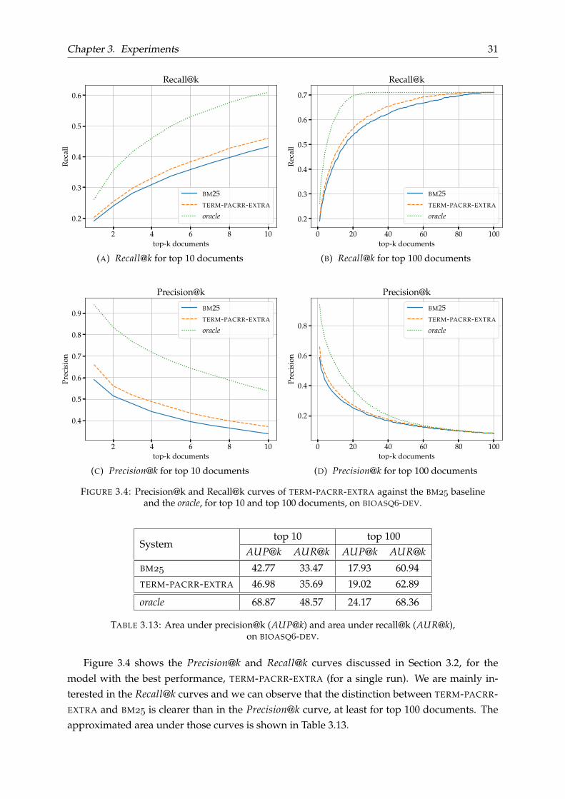
FIGURE 3.4: Precision@k and Recall@k curves of TERM-PACRR-EXTRA against the BM baselineand the oracle, for top 10 and top 100 documents, on BIOASQ-DEV.
Systemtop 10 top 100
AUP@k AUR@k AUP@k AUR@k
BM 42.77 33.47 17.93 60.94
TERM-PACRR-EXTRA 46.98 35.69 19.02 62.89
oracle 68.87 48.57 24.17 68.36
TABLE 3.13: Area under precision@k (AUP@k) and area under recall@k (AUR@k),on BIOASQ-DEV.
Figure 3.4 shows the Precision@k and Recall@k curves discussed in Section 3.2, for themodel with the best performance, TERM-PACRR-EXTRA (for a single run). We are mainly in-terested in the Recall@k curves and we can observe that the distinction between TERM-PACRR-EXTRA and BM is clearer than in the Precision@k curve, at least for top 100 documents. Theapproximated area under those curves is shown in Table 3.13.
Chapter 3. Experiments 32
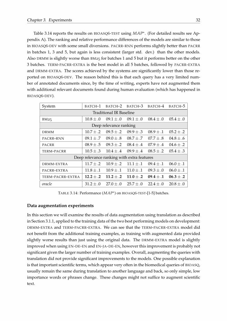
Table 3.14 reports the results on BIOASQ-TEST using MAP?. (For detailed results see Ap-pendix A). The ranking and relative performance differences of the models are similar to thosein BIOASQ-DEV with some small diversions. PACRR-RNN performs slightly better than PACRR
in batches 1, 3 and 5, but again is less consistent (larger std. dev.) than the other models.Also DRMM is slightly worse than BM for batches 1 and 5 but it performs better on the other3 batches. TERM-PACRR-EXTRA is the best model in all 5 batches, followed by PACRR-EXTRA
and DRMM-EXTRA. The scores achieved by the systems are significantly lower than those re-ported on BIOASQ-DEV. The reason behind this is that each query has a very limited num-ber of annotated documents since, by the time of writing, experts have not augmented themwith additional relevant documents found during human evaluation (which has happened inBIOASQ-DEV).
System BATCH-1 BATCH-2 BATCH-3 BATCH-4 BATCH-5
Traditional IR Baseline
BM 10.8± .0 09.1± .0 09.1± .0 08.4± .0 05.4± .0
Deep relevance ranking
DRMM 10.7± .2 09.5± .2 09.9± .3 08.9± .1 05.2± .2
PACRR-RNN 09.1± .7 09.0± .8 08.7± .7 07.7± .8 04.8± .6
PACRR 08.9± .5 09.3± .2 08.4± .4 07.9± .4 04.6± .2
TERM-PACRR 10.5± .3 10.4± .4 09.9± .4 08.5± .2 05.4± .3
Deep relevance ranking with extra features
DRMM-EXTRA 11.7± .2 10.9± .2 11.1± .1 09.4± .1 06.0± .1
PACRR-EXTRA 11.8± .1 10.9± .1 11.0± .1 09.3± .0 06.0± .1
TERM-PACRR-EXTRA 12.2± .2 11.2± .2 11.0± .2 09.4± .1 06.3± .2
oracle 31.2± .0 27.0± .0 25.7± .0 22.4± .0 20.8± .0
TABLE 3.14: Performance (MAP?) on BIOASQ-TEST-[1-5] batches.
Data augmentation experiments
In this section we will examine the results of data augmentation using translation as describedin Section 3.1.1, applied to the training data of the two best performing models on development:DRMM-EXTRA and TERM-PACRR-EXTRA. We can see that the TERM-PACRR-EXTRA model didnot benefit from the additional training examples, as training with augmented data providedslightly worse results than just using the original data. The DRMM-EXTRA model is slightlyimproved when using EN-DE-EN and EN-JA-DE-EN, however this improvement is probably notsignificant given the larger number of training examples. Overall, augmenting the queries withtranslation did not provide significant improvements to the models. One possible explanationis that important scientific terms, which appear very often in the biomedical queries of BIOASQ,usually remain the same during translation to another language and back, so only simple, lowimportance words or phrases change. These changes might not suffice to augment scientifictext.
Chapter 3. Experiments 33
System MAP? GMAP Precision Recall F-measure
DRMM-EXTRA 30.4± .2 5.8± .1 37.6± .2 45.6± .3 31.9± .2
+EN-DE-EN 30.6± .3 5.7± .2 37.8± .2 45.7± .2 32.0± .1
+EN-JA-EN 30.4± .2 5.8± .2 37.7± .2 45.5± .2 31.9± .2
+EN-JA-DE-EN 30.5± .1 5.7± .3 37.8± .2 45.6± .3 32.0± .2
TERM-PACRR-EXTRA 31.0± .2 6.1± .2 38.2± .1 46.2± .1 32.4± .1
+EN-DE-EN 30.6± .3 6.0± .2 37.9± .3 46.0± .1 32.2± .2
+EN-JA-EN 30.7± .3 6.0± .1 38.1± .2 46.2± .1 32.3± .1
+EN-JA-DE-EN 30.7± .2 6.0± .1 38.1± .2 46.2± .2 32.3± .2
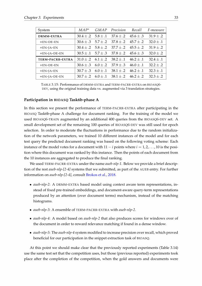
TABLE 3.15: Performance of DRMM-EXTRA and TERM-PACRR-EXTRA on BIOASQ-DEV, using the original training data vs. augmented via 3 translation strategies.
Participation in BIOASQ Task6b-phase A
In this section we present the performance of TERM-PACRR-EXTRA after participating in theBIOASQ Task6b-phase A challenge for document ranking. For the training of the model weused BIOASQ-TRAIN augmented by an additional 400 queries from the BIOASQ-DEV set. Asmall development set of the remaining 100 queries of BIOASQ-DEV was still used for epochselection. In order to moderate the fluctuations in performance due to the random initializa-tion of the network parameters, we trained 10 different instances of the model and for eachtest query the predicted document ranking was based on the following voting scheme: Eachinstance of the model votes for a document with 11− i points where i = 1, 2, . . . , 10 is the posi-tion where this document was ranked by this instance. Then the points of each document fromthe 10 instances are aggregated to produce the final ranking.
We used TERM-PACRR-EXTRA under the name aueb-nlp-1. Below we provide a brief descrip-tion of the rest aueb-nlp-[2-4] systems that we submitted, as part of the AUEB entry. For furtherinformation on aueb-nlp-[2-4], consult Brokos et al., 2018.
• aueb-nlp-2: A DRMM-EXTRA based model using context aware term representations, in-stead of fixed pre-trained embeddings, and document-aware query-term representationsproduced by an attention (over document terms) mechanism, instead of the matchinghistograms.
• aueb-nlp-3: A ensemble of TERM-PACRR-EXTRA with aueb-nlp-2.
• aueb-nlp-4: A model based on aueb-nlp-2 that also produces scores for windows over ofthe document in order to reward relevance matching if found in a dense window.
• aueb-nlp-5: The aueb-nlp-4 system modified to increase precision over recall, which provedbeneficial for our participation in the snippet extraction task of BIOASQ.
At this point we should make clear that the previously reported experiments (Table 3.14)use the same test set that the competition uses, but those (previous reported) experiments tookplace after the completion of the competition, when the gold answers and documents were
Chapter 3. Experiments 34
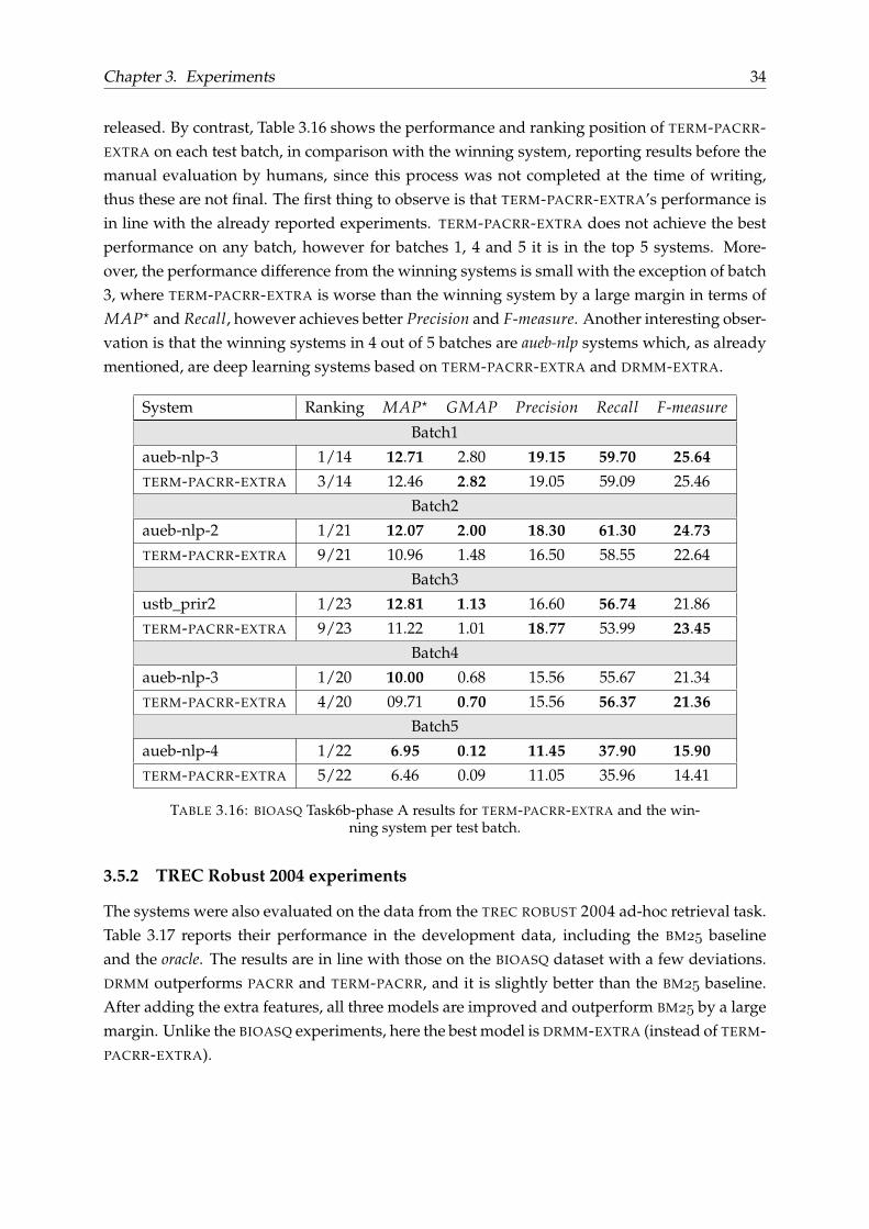
released. By contrast, Table 3.16 shows the performance and ranking position of TERM-PACRR-EXTRA on each test batch, in comparison with the winning system, reporting results before themanual evaluation by humans, since this process was not completed at the time of writing,thus these are not final. The first thing to observe is that TERM-PACRR-EXTRA’s performance isin line with the already reported experiments. TERM-PACRR-EXTRA does not achieve the bestperformance on any batch, however for batches 1, 4 and 5 it is in the top 5 systems. More-over, the performance difference from the winning systems is small with the exception of batch3, where TERM-PACRR-EXTRA is worse than the winning system by a large margin in terms ofMAP? and Recall, however achieves better Precision and F-measure. Another interesting obser-vation is that the winning systems in 4 out of 5 batches are aueb-nlp systems which, as alreadymentioned, are deep learning systems based on TERM-PACRR-EXTRA and DRMM-EXTRA.
System Ranking MAP? GMAP Precision Recall F-measure
Batch1
aueb-nlp-3 1/14 12.71 2.80 19.15 59.70 25.64TERM-PACRR-EXTRA 3/14 12.46 2.82 19.05 59.09 25.46
Batch2
aueb-nlp-2 1/21 12.07 2.00 18.30 61.30 24.73TERM-PACRR-EXTRA 9/21 10.96 1.48 16.50 58.55 22.64
Batch3
ustb_prir2 1/23 12.81 1.13 16.60 56.74 21.86
TERM-PACRR-EXTRA 9/23 11.22 1.01 18.77 53.99 23.45Batch4
aueb-nlp-3 1/20 10.00 0.68 15.56 55.67 21.34
TERM-PACRR-EXTRA 4/20 09.71 0.70 15.56 56.37 21.36Batch5
aueb-nlp-4 1/22 6.95 0.12 11.45 37.90 15.90TERM-PACRR-EXTRA 5/22 6.46 0.09 11.05 35.96 14.41
TABLE 3.16: BIOASQ Task6b-phase A results for TERM-PACRR-EXTRA and the win-ning system per test batch.
3.5.2 TREC Robust 2004 experiments
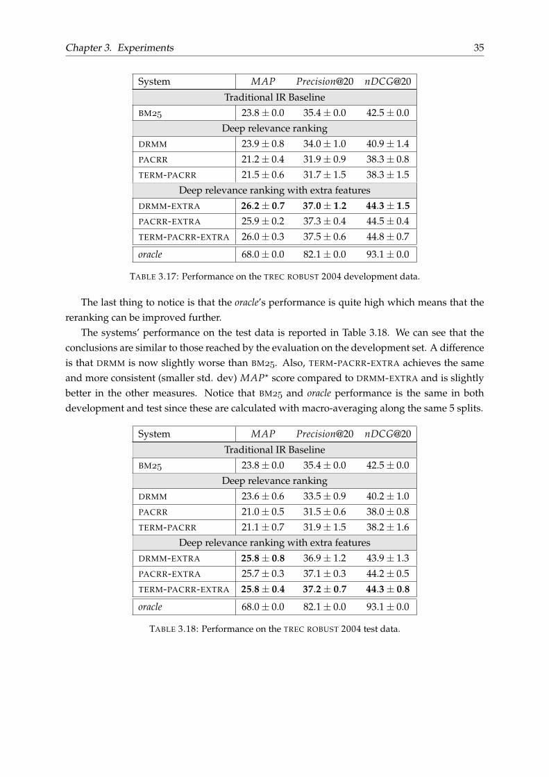
The systems were also evaluated on the data from the TREC ROBUST 2004 ad-hoc retrieval task.Table 3.17 reports their performance in the development data, including the BM baselineand the oracle. The results are in line with those on the BIOASQ dataset with a few deviations.DRMM outperforms PACRR and TERM-PACRR, and it is slightly better than the BM baseline.After adding the extra features, all three models are improved and outperform BM by a largemargin. Unlike the BIOASQ experiments, here the best model is DRMM-EXTRA (instead of TERM-PACRR-EXTRA).
Chapter 3. Experiments 35
System MAP Precision@20 nDCG@20
Traditional IR Baseline
BM 23.8± 0.0 35.4± 0.0 42.5± 0.0
Deep relevance ranking
DRMM 23.9± 0.8 34.0± 1.0 40.9± 1.4
PACRR 21.2± 0.4 31.9± 0.9 38.3± 0.8
TERM-PACRR 21.5± 0.6 31.7± 1.5 38.3± 1.5
Deep relevance ranking with extra features
DRMM-EXTRA 26.2± 0.7 37.0± 1.2 44.3± 1.5PACRR-EXTRA 25.9± 0.2 37.3± 0.4 44.5± 0.4
TERM-PACRR-EXTRA 26.0± 0.3 37.5± 0.6 44.8± 0.7
oracle 68.0± 0.0 82.1± 0.0 93.1± 0.0
TABLE 3.17: Performance on the TREC ROBUST 2004 development data.
The last thing to notice is that the oracle’s performance is quite high which means that thereranking can be improved further.
The systems’ performance on the test data is reported in Table 3.18. We can see that theconclusions are similar to those reached by the evaluation on the development set. A differenceis that DRMM is now slightly worse than BM. Also, TERM-PACRR-EXTRA achieves the sameand more consistent (smaller std. dev) MAP? score compared to DRMM-EXTRA and is slightlybetter in the other measures. Notice that BM and oracle performance is the same in bothdevelopment and test since these are calculated with macro-averaging along the same 5 splits.
System MAP Precision@20 nDCG@20
Traditional IR Baseline
BM 23.8± 0.0 35.4± 0.0 42.5± 0.0
Deep relevance ranking
DRMM 23.6± 0.6 33.5± 0.9 40.2± 1.0
PACRR 21.0± 0.5 31.5± 0.6 38.0± 0.8
TERM-PACRR 21.1± 0.7 31.9± 1.5 38.2± 1.6
Deep relevance ranking with extra features
DRMM-EXTRA 25.8± 0.8 36.9± 1.2 43.9± 1.3
PACRR-EXTRA 25.7± 0.3 37.1± 0.3 44.2± 0.5
TERM-PACRR-EXTRA 25.8± 0.4 37.2± 0.7 44.3± 0.8
oracle 68.0± 0.0 82.1± 0.0 93.1± 0.0
TABLE 3.18: Performance on the TREC ROBUST 2004 test data.
36
Chapter 4
Related Work
Document relevance ranking is a standard problem in information retrieval, widely studiedover the years. Traditional approaches consist of term weighting schemes (Robertson andJones, 1988), and methods based on statistical NLP like the query likelihood model (Ponte andCroft, 1998) that scores each document by the probability assigned to a query by the statisti-cal language model of the document. Another method, extensively used and described in thisthesis, that is derived from probabilistic methods of relevance ranking is BM (Robertson andZaragoza, 2009).
The recent outbreak of deep learning has lead to state-of-the-art results in various NLP tasks,influencing the research in deep learning for document relevance ranking (Zhang et al., 2016;Onal et al., 2017; Craswell et al., 2018). One of the first successful works is the DSSM model ofHuang et al., 2013. DSSM first hashes a query or a document, in sparse vectors that indicatethe n-grams contained in its text, similarly to term level sparse vectors that are widely usedin conventional IR to represent documents, but using significantly fewer dimensions. Thesehashed query and document representations are then passed through multiple non-linear lay-ers to produce high level, low dimensional representations for a query and each candidatedocument. Then, cosine similarity between the query and each document representation isused as the documents’ relevance scores. The model is trained using click-through data, bymaximizing the likelihood (relevance score) of the clicked documents given the query.
An extension of this model is CLSM (or CDSSM) of Shen et al., 2014, which applies convolu-tion to the hashed term representations to obtain contextual information and then applies maxpooling to aggregate the output of each convolution into a vector that represents a query ordocument. This vector is then passed though a single non-linear layer to produce the final highlevel representation.
The advent of large-scale word embeddings (Mikolov et al., 2013; Pennington et al., 2014),opened the way for new relevance ranking models that utilize these rich term representationsinstead of the conventional sparse vectors. Two of these models is the DRMM model of Guoet al., 2016 and the PACRR model of Hui et al., 2017 that were analyzed and used in this thesis.Another model is K-NRM of Xiong et al., 2017 which first calculates a translation matrix contain-ing word to word similarities or word embeddings (similar to PACRR’s similarity matrix) andthen applies multiple (k) kernels to each row, to produce a document dependent representation(k-dimensional) for each query term. Then the representations of all query terms are aggre-gated through logarithm of their summation and the resulting query-document representation
Chapter 4. Related Work 37
passes through a non-linear layer to produce the relevance score. The model is trained usinghinge loss on pairs of relevant and non-relevant documents, given a query.
A different approach to the widely used query-document interaction matrix is that of Jaechet al., 2017. First, the word embeddings of a query q and a document d pass through separatebidirectional LSTMs. A linear projection matrix is applied to the hidden states of both BI-LSTMs,to obtain term representations with the same dimensionality k. In contrast to PACRR, K-NRM
and other works, Jaech et al., 2017 use element-wise (Hadamard) product between each queryand each document term vector resulting in a (|q| × |d| × k) 3-D Match-Tensor. An extra di-mension is added (k + 1) containing binary exact matching signals. Subsequently, multiple 3-Dconvolutions are applied to the matching tensor and the outputs of max pooling for each ofthose are aggregated into a final query-document representation vector that is passed througha fully-connected layer to produce a relevance score.
The main evaluation in this thesis utilized data of the biomedical domain. A related workon biomedical IR using deep learning is this of Mohan et al., 2017. As a first stage, the proposedmodel computes simple interactions between each document term and its closest, in terms ofEuclidean distance, query term. After applying convolution to these interactions and max pool-ing, the resulting document-query representation is combined with overlap features similar tothose used in this thesis. The combined vector then passes through an MLP to produce a rele-vance score. An important distinction of this work with ours is that it utilizes click-though datafrom PubMed, instead of a relatively small training dataset like the one we used from BIOASQ.
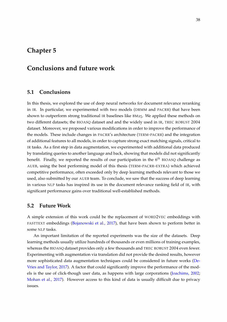
38
Chapter 5
Conclusions and future work
5.1 Conclusions
In this thesis, we explored the use of deep neural networks for document relevance rerankingin IR. In particular, we experimented with two models (DRMM and PACRR) that have beenshown to outperform strong traditional IR baselines like BM. We applied these methods ontwo different datasets; the BIOASQ dataset and and the widely used in IR, TREC ROBUST 2004dataset. Moreover, we proposed various modifications in order to improve the performance ofthe models. These include changes in PACRR’s architecture (TERM-PACRR) and the integrationof additional features to all models, in order to capture strong exact matching signals, critical toIR tasks. As a first step in data augmentation, we experimented with additional data producedby translating queries to another language and back, showing that models did not significantlybenefit. Finally, we reported the results of our participation in the 6th BIOASQ challenge asAUEB, using the best performing model of this thesis (TERM-PACRR-EXTRA) which achievedcompetitive performance, often exceeded only by deep learning methods relevant to those weused, also submitted by our AUEB team. To conclude, we saw that the success of deep learningin various NLP tasks has inspired its use in the document relevance ranking field of IR, withsignificant performance gains over traditional well-established methods.
5.2 Future Work
A simple extension of this work could be the replacement of WORD2VEC embeddings withFASTTEXT embeddings (Bojanowski et al., 2017), that have been shown to perform better insome NLP tasks.
An important limitation of the reported experiments was the size of the datasets. Deeplearning methods usually utilize hundreds of thousands or even millions of training examples,whereas the BIOASQ dataset provides only a few thousands and TREC ROBUST 2004 even fewer.Experimenting with augmentation via translation did not provide the desired results, howevermore sophisticated data augmentation techniques could be considered in future works (De-Vries and Taylor, 2017). A factor that could significantly improve the performance of the mod-els is the use of click-though user data, as happens with large corporations (Joachims, 2002;Mohan et al., 2017). However access to this kind of data is usually difficult due to privacyissues.

Chapter 5. Conclusions and future work 39
Finally, the models used in this thesis belong to the interaction-focused category, whichmakes it difficult to index documents and perform full document retrieval. Representation-focused models that use attention mechanisms (Bahdanau et al., 2015) could be considered inorder to both capture strong exact or near matching signals and make it possible to producequery independent document representations that can be indexed and retrieved during searchtime, without having to use a reranking strategy.
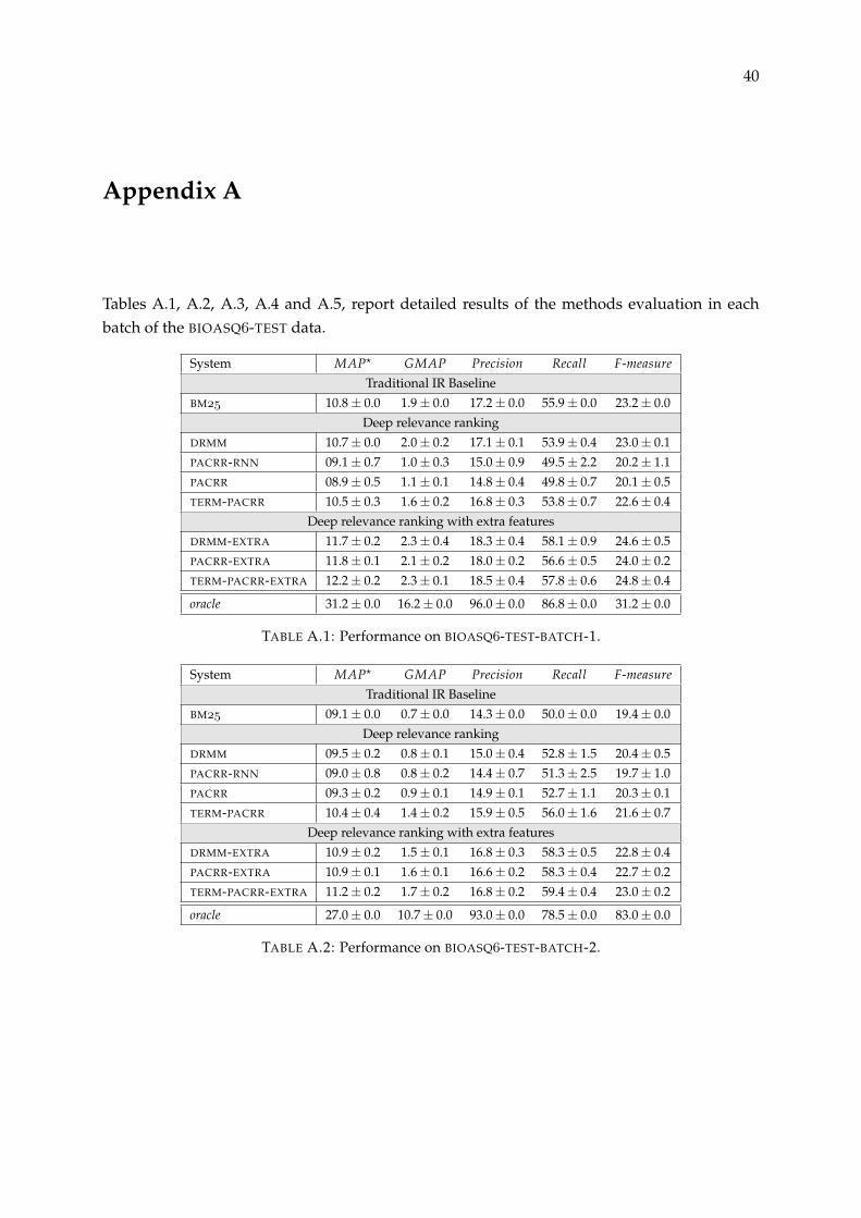
40
Appendix A
Tables A.1, A.2, A.3, A.4 and A.5, report detailed results of the methods evaluation in eachbatch of the BIOASQ-TEST data.
System MAP? GMAP Precision Recall F-measureTraditional IR Baseline
BM 10.8± 0.0 1.9± 0.0 17.2± 0.0 55.9± 0.0 23.2± 0.0Deep relevance ranking
DRMM 10.7± 0.0 2.0± 0.2 17.1± 0.1 53.9± 0.4 23.0± 0.1PACRR-RNN 09.1± 0.7 1.0± 0.3 15.0± 0.9 49.5± 2.2 20.2± 1.1PACRR 08.9± 0.5 1.1± 0.1 14.8± 0.4 49.8± 0.7 20.1± 0.5TERM-PACRR 10.5± 0.3 1.6± 0.2 16.8± 0.3 53.8± 0.7 22.6± 0.4
Deep relevance ranking with extra featuresDRMM-EXTRA 11.7± 0.2 2.3± 0.4 18.3± 0.4 58.1± 0.9 24.6± 0.5PACRR-EXTRA 11.8± 0.1 2.1± 0.2 18.0± 0.2 56.6± 0.5 24.0± 0.2TERM-PACRR-EXTRA 12.2± 0.2 2.3± 0.1 18.5± 0.4 57.8± 0.6 24.8± 0.4
oracle 31.2± 0.0 16.2± 0.0 96.0± 0.0 86.8± 0.0 31.2± 0.0
TABLE A.1: Performance on BIOASQ-TEST-BATCH-1.
System MAP? GMAP Precision Recall F-measureTraditional IR Baseline
BM 09.1± 0.0 0.7± 0.0 14.3± 0.0 50.0± 0.0 19.4± 0.0Deep relevance ranking
DRMM 09.5± 0.2 0.8± 0.1 15.0± 0.4 52.8± 1.5 20.4± 0.5PACRR-RNN 09.0± 0.8 0.8± 0.2 14.4± 0.7 51.3± 2.5 19.7± 1.0PACRR 09.3± 0.2 0.9± 0.1 14.9± 0.1 52.7± 1.1 20.3± 0.1TERM-PACRR 10.4± 0.4 1.4± 0.2 15.9± 0.5 56.0± 1.6 21.6± 0.7
Deep relevance ranking with extra featuresDRMM-EXTRA 10.9± 0.2 1.5± 0.1 16.8± 0.3 58.3± 0.5 22.8± 0.4PACRR-EXTRA 10.9± 0.1 1.6± 0.1 16.6± 0.2 58.3± 0.4 22.7± 0.2TERM-PACRR-EXTRA 11.2± 0.2 1.7± 0.2 16.8± 0.2 59.4± 0.4 23.0± 0.2
oracle 27.0± 0.0 10.7± 0.0 93.0± 0.0 78.5± 0.0 83.0± 0.0
TABLE A.2: Performance on BIOASQ-TEST-BATCH-2.
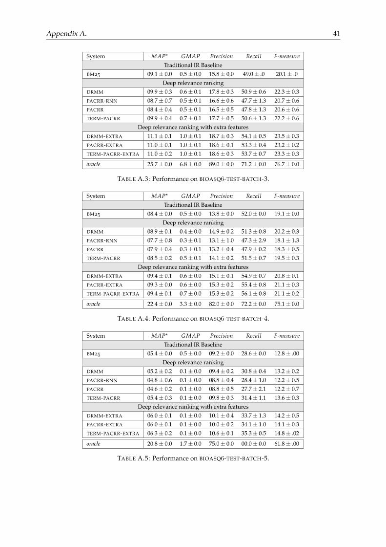
Appendix A. 41
System MAP? GMAP Precision Recall F-measureTraditional IR Baseline
BM 09.1± 0.0 0.5± 0.0 15.8± 0.0 49.0± .0 20.1± .0Deep relevance ranking
DRMM 09.9± 0.3 0.6± 0.1 17.8± 0.3 50.9± 0.6 22.3± 0.3PACRR-RNN 08.7± 0.7 0.5± 0.1 16.6± 0.6 47.7± 1.3 20.7± 0.6PACRR 08.4± 0.4 0.5± 0.1 16.5± 0.5 47.8± 1.3 20.6± 0.6TERM-PACRR 09.9± 0.4 0.7± 0.1 17.7± 0.5 50.6± 1.3 22.2± 0.6
Deep relevance ranking with extra featuresDRMM-EXTRA 11.1± 0.1 1.0± 0.1 18.7± 0.3 54.1± 0.5 23.5± 0.3PACRR-EXTRA 11.0± 0.1 1.0± 0.1 18.6± 0.1 53.3± 0.4 23.2± 0.2TERM-PACRR-EXTRA 11.0± 0.2 1.0± 0.1 18.6± 0.3 53.7± 0.7 23.3± 0.3
oracle 25.7± 0.0 6.8± 0.0 89.0± 0.0 71.2± 0.0 76.7± 0.0
TABLE A.3: Performance on BIOASQ-TEST-BATCH-3.
System MAP? GMAP Precision Recall F-measureTraditional IR Baseline
BM 08.4± 0.0 0.5± 0.0 13.8± 0.0 52.0± 0.0 19.1± 0.0Deep relevance ranking
DRMM 08.9± 0.1 0.4± 0.0 14.9± 0.2 51.3± 0.8 20.2± 0.3PACRR-RNN 07.7± 0.8 0.3± 0.1 13.1± 1.0 47.3± 2.9 18.1± 1.3PACRR 07.9± 0.4 0.3± 0.1 13.2± 0.4 47.9± 0.2 18.3± 0.5TERM-PACRR 08.5± 0.2 0.5± 0.1 14.1± 0.2 51.5± 0.7 19.5± 0.3
Deep relevance ranking with extra featuresDRMM-EXTRA 09.4± 0.1 0.6± 0.0 15.1± 0.1 54.9± 0.7 20.8± 0.1PACRR-EXTRA 09.3± 0.0 0.6± 0.0 15.3± 0.2 55.4± 0.8 21.1± 0.3TERM-PACRR-EXTRA 09.4± 0.1 0.7± 0.0 15.3± 0.2 56.1± 0.8 21.1± 0.2
oracle 22.4± 0.0 3.3± 0.0 82.0± 0.0 72.2± 0.0 75.1± 0.0
TABLE A.4: Performance on BIOASQ-TEST-BATCH-4.
System MAP? GMAP Precision Recall F-measureTraditional IR Baseline
BM 05.4± 0.0 0.5± 0.0 09.2± 0.0 28.6± 0.0 12.8± .00Deep relevance ranking
DRMM 05.2± 0.2 0.1± 0.0 09.4± 0.2 30.8± 0.4 13.2± 0.2PACRR-RNN 04.8± 0.6 0.1± 0.0 08.8± 0.4 28.4± 1.0 12.2± 0.5PACRR 04.6± 0.2 0.1± 0.0 08.8± 0.5 27.7± 2.1 12.2± 0.7TERM-PACRR 05.4± 0.3 0.1± 0.0 09.8± 0.3 31.4± 1.1 13.6± 0.3
Deep relevance ranking with extra featuresDRMM-EXTRA 06.0± 0.1 0.1± 0.0 10.1± 0.4 33.7± 1.3 14.2± 0.5PACRR-EXTRA 06.0± 0.1 0.1± 0.0 10.0± 0.2 34.1± 1.0 14.1± 0.3TERM-PACRR-EXTRA 06.3± 0.2 0.1± 0.0 10.6± 0.1 35.3± 0.5 14.8± .02
oracle 20.8± 0.0 1.7± 0.0 75.0± 0.0 00.0± 0.0 61.8± .00
TABLE A.5: Performance on BIOASQ-TEST-BATCH-5.
42
Bibliography
D. Bahdanau, K. Cho, and Y. Bengio (2015). “Neural Machine Translation by Jointly Learningto Align and Translate”. In: In Proceedings of the 3rd International Conference on Learning Rep-resentations (ICLR). San Diego, CA.
P. Bojanowski, E. Grave, A. Joulin, and T. Mikolov (2017). “Enriching Word Vectors with Sub-word Information”. In: Transactions of the Association for Computational Linguistics (TACL) 5,pp. 135–146.
G. Brokos, P. Malakasiotis, and I. Androutsopoulos (2016). “Using Centroids of Word Embed-dings and Word Mover’s Distance for Biomedical Document Retrieval in Question Answer-ing”. In: Proceedings of the 15th Workshop on Biomedical Natural Language Processing (BioNLP),at the 54th Annual Meeting of the Association for Computational Linguistics (ACL). Berlin, Ger-many, pp. 114–118.
G. Brokos, P. Liosis, R. McDonald, D. Pappas, and I. Androutsopoulos (2018). “AUEB at BioASQ6: Document and Snippet Retrieval”. Under review.
J. Bromley, I. Guyon, Y. LeCun, E. Säckinger, and R. Shah (1993). “Signature Verification Usinga "Siamese" Time Delay Neural Network”. In: Proceedings of the 6th International Conferenceon Neural Information Processing Systems. San Francisco, CA, pp. 737–744.
N. Craswell, W. B. Croft, M. de Rijke, J. Guo, and B. Mitra (2018). “Neural information retrieval:introduction to the special issue”. In: Information Retrieval Journal 21.2, pp. 107–110.
T. DeVries and G. W. Taylor (2017). “Dataset Augmentation in Feature Space”. In: ArXiv e-prints.arXiv: 1702.05538 [stat.ML].
X. Glorot and Y. Bengio (2010). “Understanding the difficulty of training deep feedforward neu-ral networks”. In: Proceedings of the Thirteenth International Conference on Artificial Intelligenceand Statistics. Sardinia, Italy, pp. 249–256.
J. Guo, Y. Fan, Q. Ai, and W. B. Croft (2016). “A Deep Relevance Matching Model for Ad-hoc Retrieval”. In: Proceedings of the 25th ACM International Conference on Information andKnowledge Management (CIKM). Indianapolis, IN, pp. 55–64.
S. Hochreiter and J. Schmidhuber (1997). “Long Short-Term Memory”. In: Neural Computation9.8, pp. 1735–1780.
P. Huang, X. He, J. Gao, L. Deng, A. Acero, and L. Heck (2013). “Learning Deep StructuredSemantic Models for Web Search Using Clickthrough Data”. In: Proceedings of the 22nd ACMInternational Conference on Information & Knowledge Management (CIKM). San Francisco, CA,pp. 2333–2338.
K. Hui, A. Yates, K. Berberich, and G. de Melo (2017). “PACRR: A Position-Aware Neural IRModel for Relevance Matching”. In: Proceedings of the 2017 Conference on Empirical Methodsin Natural Language Processing (EMNLP). Copenhagen, Denmark, pp. 1060–1069.
BIBLIOGRAPHY 43
K. Hui, A. Yates, K. Berberich, and G. de Melo (2018). “Co-PACRR: A Context-Aware NeuralIR Model for Ad-hoc Retrieval”. In: Proceedings of the Eleventh ACM International Conferenceon Web Search and Data Mining. Marina Del Rey, CA, pp. 279–287.
A. Jaech, H. Kamisetty, E. K. Ringger, and C. Clarke (2017). “Match-Tensor: a Deep RelevanceModel for Search”. In: ArXiv e-prints. arXiv: 1701.07795 [cs.IR].
T. Joachims (2002). “Optimizing search engines using clickthrough data”. In: Proceedings of the8th ACM SIGKDD International Conference on Knowledge Discovery and Data Mining. Edmon-ton, Canada, pp. 133–142.
D. P. Kingma and J. Ba (2014). “Adam: A Method for Stochastic Optimization”. In: ArXiv e-prints. arXiv: 1412.6980 [cs.LG].
J. M. Kleinberg (1999). “Authoritative sources in a hyperlinked environment”. In: Journal of theACM (JACM) 46.5, pp. 604–632.
R. Krovetz (1993). “Viewing Morphology As an Inference Process”. In: Proceedings of the 16thAnnual International ACM SIGIR Conference on Research and Development in Information Re-trieval. Pittsburgh, PA, pp. 191–202.
P. Malakasiotis, I. Pavlopoulos, I. Androutsopoulos, and A. Nentidis (2018). Evaluation Measuresfor Task B. Tech. rep. BioASQ.
C. D. Manning, P. Raghavan, and H. Schütze (2008). Introduction to Information Retrieval. Cam-bridge University Press.
T. Mikolov, I. Sutskever, K. Chen, G. Corrado, and J. Dean (2013). “Distributed Representationsof Words and Phrases and their Compositionality”. In: Proceedings of the 26th InternationalConference on Neural Information Processing Systems. Vol. 2. Lake Tahoe, NV, pp. 3111–3119.
S. Mohan, N. Fiorini, S. Kim, and Z.Lu (2017). “Deep Learning for Biomedical InformationRetrieval: Learning Textual Relevance from Click Logs”. In: Proceedings of the 16th BioNLPWorkshop. Vancouver, Canada, pp. 222–231.
K. D. Onal, Y. Zhang, I. S. Altingövde, M. Rahman, P. Senkul, A. Braylan, B. Dang, H.-L. Chang,H. Kim, Q. McNamara, A. Angert, E. Banner, V. Khetan, T. McDonnell, A. T. Nguyen, D. Xu,B. C. Wallace, M. de Rijke, and M. Lease (2017). “Neural information retrieval: at the end ofthe early years”. In: Information Retrieval Journal 21.2-3, pp. 111–182.
L. Page, S. Brin, R. Motwani, and T. Winograd (1999). The PageRank citation ranking: Bringingorder to the web. Tech. rep. Stanford InfoLab.
J. Pennington, R. Socher, and C. D. Manning (2014). “Glove: Global Vectors for Word Repre-sentation”. In: Proceedings of the 2014 Conference on Empirical Methods in Natural LanguageProcessing (EMNLP). Doha, Qatar, pp. 1532–1543.
J. M. Ponte and W. B. Croft (1998). “A Language Modeling Approach to Information Retrieval”.In: Proceedings of the 21st Annual International ACM SIGIR Conference on Research and Devel-opment in Information Retrieval. Melbourne, Australia, pp. 275–281.
S. Robertson and K. Sparck Jones (1988). “Document Retrieval Systems”. In: ed. by Peter Willett.London, UK: Taylor Graham Publishing. Chap. "Relevance Weighting of Search Terms",pp. 143–160.
S. Robertson and H. Zaragoza (2009). “The probabilistic relevance framework: BM25 and be-yond”. In: Foundations and Trends in Information Retrieval 3.4, pp. 333–389.
BIBLIOGRAPHY 44
S. Robertson, S. Walker, S. Jones, M. M. Hancock-Beaulieu, and M. Gatford (1995). “Okapi atTREC–3”. In: Overview of the Third Text REtrieval Conference (TREC–3), pp. 109–126.
A. Severyn and A. Moschitti (2015). “Learning to Rank Short Text Pairs with ConvolutionalDeep Neural Networks”. In: Proceedings of the 38th International ACM SIGIR Conference onResearch and Development in Information Retrieval. Santiago, Chile, pp. 373–382.
Y. Shen, X. He, J. Gao, L. Deng, and G. Mesnil (2014). “A Latent Semantic Model withConvolutional-Pooling Structure for Information Retrieval”. In: Proceedings of the 23rd ACMInternational Conference on Conference on Information and Knowledge Management (CIKM). Shang-hai, China, pp. 101–110.
G. Tsatsaronis, G. Balikas, P. Malakasiotis, I. Partalas, M. Zschunke, M. R. Alvers, D. Weis-senborn, A. Krithara, S. Petridis, D. Polychronopoulos, Y. Almirantis, J. Pavlopoulos, N.Baskiotis, P. Gallinari, T. Artiéres, A.-C. N. Ngomo, N. Heino, E. Gaussier, L. Barrio-Alvers,M. Schroeder, I. Androutsopoulos, and G. Paliouras (2015). “An overview of the BIOASQlarge-scale biomedical semantic indexing and question answering competition”. In: BMCBioinformatics 16.1, p. 138.
E. M. Voorhees (2005). “The TREC robust retrieval track”. In: ACM SIGIR Forum 39.1, pp. 11–20.C. Xiong, Z. Dai, J. Callan, Z. Liu, and R. Power (2017). “End-to-End Neural Ad-hoc Rank-
ing with Kernel Pooling”. In: Proceedings of the 40th International ACM SIGIR Conference onResearch and Development in Information Retrieval. Shinjuku, Tokyo, Japan, pp. 55–64.
Y. Zhang, M. Mustafizur Rahman, A. Braylan, B. Dang, H.-L. Chang, H. Kim, Q. McNamara,A. Angert, E. Banner, V. Khetan, T. McDonnell, A. Thanh Nguyen, D. Xu, B. C. Wallace, andM. Lease (2016). “Neural Information Retrieval: A Literature Review”. In: ArXiv e-prints.arXiv: 1611.06792 [cs.IR].