Density Functional Theory - Rutgers Physics & Astronomyhaule/681/DFT.pdf · 2017-11-29 · KH...
32
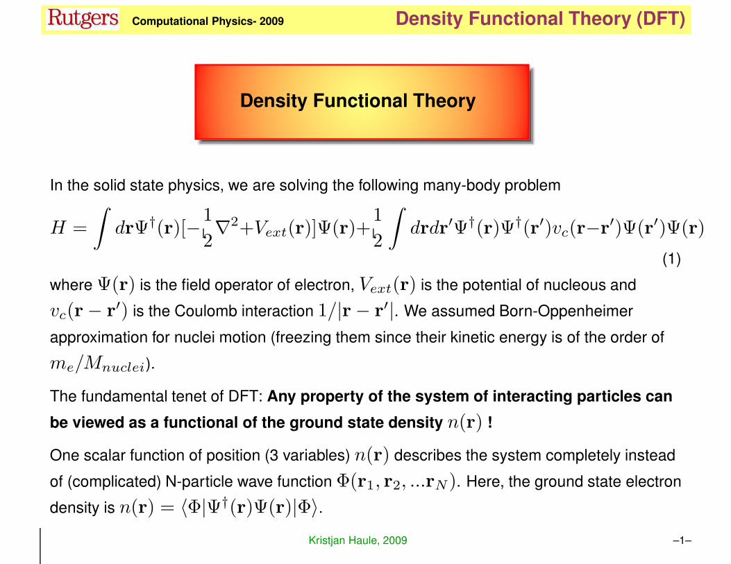
KH Computational Physics- 2009 Density Functional Theory (DFT) Density Functional Theory In the solid state physics, we are solving the following many-body problem H = drΨ † (r)[− 1 2 ∇ 2 +V ext (r)]Ψ(r)+ 1 2 drdr ′ Ψ † (r)Ψ † (r ′ )v c (r−r ′ )Ψ(r ′ )Ψ(r) (1) where Ψ(r) is the field operator of electron, V ext (r) is the potential of nucleous and v c (r − r ′ ) is the Coulomb interaction 1/|r − r ′ |. We assumed Born-Oppenheimer approximation for nuclei motion (freezing them since their kinetic energy is of the order of m e /M nuclei ). The fundamental tenet of DFT: Any property of the system of interacting particles can be viewed as a functional of the ground state density n(r) ! One scalar function of position (3 variables) n(r) describes the system completely instead of (complicated) N-particle wave function Φ(r 1 , r 2 ,...r N ). Here, the ground state electron density is n(r)= 〈Φ|Ψ † (r)Ψ(r)|Φ〉. Kristjan Haule, 2009 –1–
Transcript of Density Functional Theory - Rutgers Physics & Astronomyhaule/681/DFT.pdf · 2017-11-29 · KH...
KH Computational Physics- 2009 Density Functional Theory (DFT)
Density Functional Theory
In the solid state physics, we are solving the following many-body problem
H =
∫
drΨ†(r)[−1
2∇2+Vext(r)]Ψ(r)+
1
2
∫
drdr′Ψ†(r)Ψ†(r′)vc(r−r′)Ψ(r′)Ψ(r)
(1)
where Ψ(r) is the field operator of electron, Vext(r) is the potential of nucleous and
vc(r− r′) is the Coulomb interaction 1/|r− r
′|. We assumed Born-Oppenheimer
approximation for nuclei motion (freezing them since their kinetic energy is of the order of
me/Mnuclei).
The fundamental tenet of DFT: Any property of the system of interacting particles can
be viewed as a functional of the ground state density n(r) !
One scalar function of position (3 variables) n(r) describes the system completely instead
of (complicated) N-particle wave function Φ(r1, r2, ...rN). Here, the ground state electron
density is n(r) = 〈Φ|Ψ†(r)Ψ(r)|Φ〉.Kristjan Haule, 2009 –1–
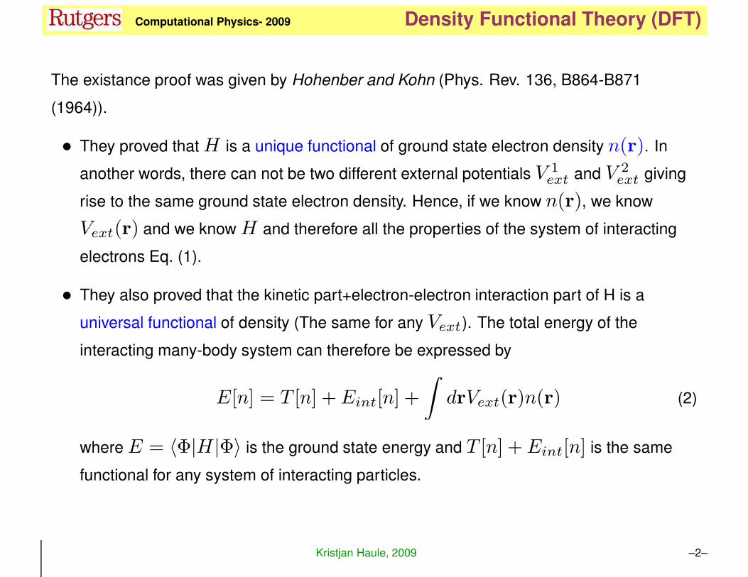
KH Computational Physics- 2009 Density Functional Theory (DFT)
The existance proof was given by Hohenber and Kohn (Phys. Rev. 136, B864-B871
(1964)).
• They proved thatH is a unique functional of ground state electron density n(r). In
another words, there can not be two different external potentials V 1ext and V 2
ext giving
rise to the same ground state electron density. Hence, if we know n(r), we know
Vext(r) and we know H and therefore all the properties of the system of interacting
electrons Eq. (1).
• They also proved that the kinetic part+electron-electron interaction part of H is a
universal functional of density (The same for any Vext). The total energy of the
interacting many-body system can therefore be expressed by
E[n] = T [n] + Eint[n] +
∫
drVext(r)n(r) (2)
where E = 〈Φ|H|Φ〉 is the ground state energy and T [n] + Eint[n] is the same
functional for any system of interacting particles.
Kristjan Haule, 2009 –2–
KH Computational Physics- 2009 Density Functional Theory (DFT)
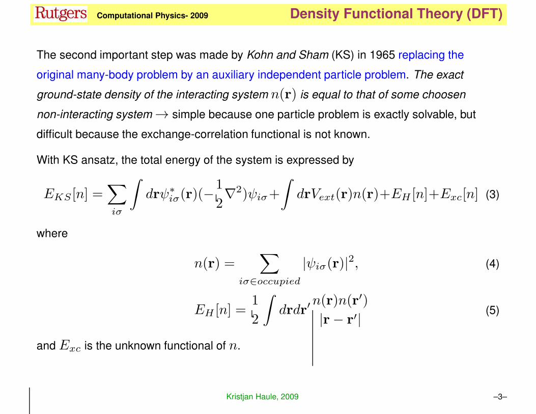
The second important step was made by Kohn and Sham (KS) in 1965 replacing the
original many-body problem by an auxiliary independent particle problem. The exact
ground-state density of the interacting system n(r) is equal to that of some choosen
non-interacting system → simple because one particle problem is exactly solvable, but
difficult because the exchange-correlation functional is not known.
With KS ansatz, the total energy of the system is expressed by
EKS [n] =∑
iσ
∫
drψ∗iσ(r)(−
1
2∇2)ψiσ+
∫
drVext(r)n(r)+EH [n]+Exc[n] (3)
where
n(r) =∑
iσ∈occupied
|ψiσ(r)|2, (4)
EH [n] =1
2
∫
drdr′n(r)n(r′)
|r− r′| (5)
and Exc is the unknown functional of n.
Kristjan Haule, 2009 –3–
KH Computational Physics- 2009 Density Functional Theory (DFT)
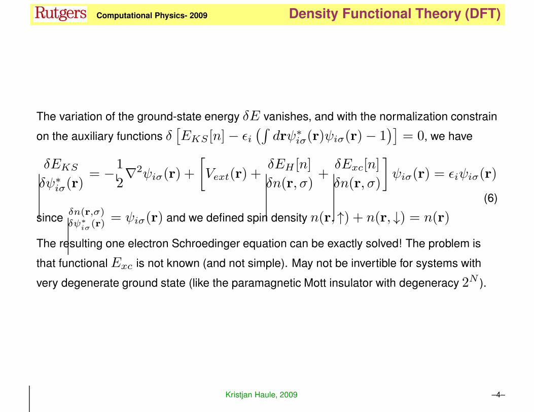
The variation of the ground-state energy δE vanishes, and with the normalization constrain
on the auxiliary functions δ[
EKS [n]− ǫi(∫
drψ∗iσ(r)ψiσ(r)− 1
)]
= 0, we have
δEKSδψ∗
iσ(r)= −1
2∇2ψiσ(r) +
[
Vext(r) +δEH [n]
δn(r, σ)+δExc[n]
δn(r, σ)
]
ψiσ(r) = ǫiψiσ(r)
(6)
sinceδn(r,σ)δψ∗
iσ(r) = ψiσ(r) and we defined spin density n(r, ↑) + n(r, ↓) = n(r)
The resulting one electron Schroedinger equation can be exactly solved! The problem is
that functionalExc is not known (and not simple). May not be invertible for systems with
very degenerate ground state (like the paramagnetic Mott insulator with degeneracy 2N ).
Kristjan Haule, 2009 –4–
KH Computational Physics- 2009 Density Functional Theory (DFT)
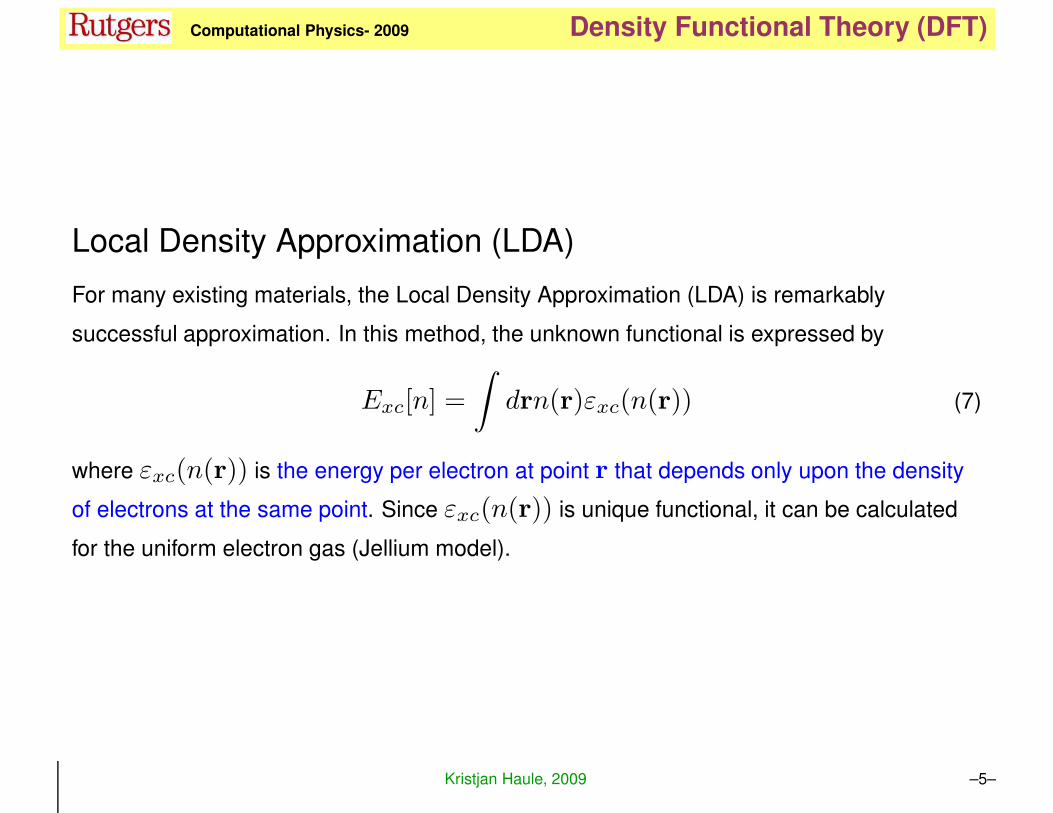
Local Density Approximation (LDA)
For many existing materials, the Local Density Approximation (LDA) is remarkably
successful approximation. In this method, the unknown functional is expressed by
Exc[n] =
∫
drn(r)εxc(n(r)) (7)
where εxc(n(r)) is the energy per electron at point r that depends only upon the density
of electrons at the same point. Since εxc(n(r)) is unique functional, it can be calculated
for the uniform electron gas (Jellium model).
Kristjan Haule, 2009 –5–
KH Computational Physics- 2009 Density Functional Theory (DFT)
The question arises
For any ground state density of an interacting electron system, is it possible to reproduce
the density exactly as the ground state density of the non-interacting electron system?
It turns out that this is not necessary the case ! There are counterexamples. However, it
works reasonably well for many systems. Counterexample: Mott insulator with 2n
degeneracy per site.
The Local Density Approximation is very successful for ”wide-band” systems with open s
and p orbitals and sometimes also for d systems. It works also for band insulators but tends
to fails in strongly correlated systems (with active d and f orbitals). The reason is that the
DFT functional becomes almost degenerate and non-invertible. With the available
approximate functionals (LDA,GGA) the ill-post problem of invertability becomes hard to
overcome.
In this case it might not be a good idea to look at the functional of the density only, but of
the energy dependent density, i.e., the Green’s function. The Luttinger-Ward functional is
one such generalization of the functional to the functional of the Green’s function (rather
than density).
One such method that can improve on LDA locality is the Dynamical Mean Field Theory
Kristjan Haule, 2009 –6–
KH Computational Physics- 2009 Density Functional Theory (DFT)
(DMFT) and its combination with LDA, dubbed LDA+DMFT method. The idea is that the
free energy functional of the system can be expressed by the local Green’s function Gω(r)
rather by the density n(r) being the static analog n(r) = Triω[Giω(r)]. The local ansatz
in this case includes important retardation effects and can be used also for the systems
with strong correlations.
The problem is that the auxiliary system remains a many-body problem (although simplified
in a form of a quantum impurity) and is much more involved than the non-interacting
Kohn-Sham problem. For more information see Rev. Mod. Phys., Kotliar et.al. 2006.
Kristjan Haule, 2009 –7–
KH Computational Physics- 2009 Density Functional Theory (DFT)
Which properties can be exactly calculated in KS formulation provided the XC functional is
known?
ground state propertis among others
• ground state energy
• ground state density
• ground state spin density
• static charge and spin susceptibility
The properties which can not be exactly calculated within KS formulation even if the XC
functional is known
• the Fermi surface and therefore Mott insulator
• excitation energies and density of states
• the size of the gaps (of insulators and semiconductors)
Surprisingly, many times even these properties are in reasonable agreement with
experiments.
Kristjan Haule, 2009 –8–
KH Computational Physics- 2009 Density Functional Theory (DFT)
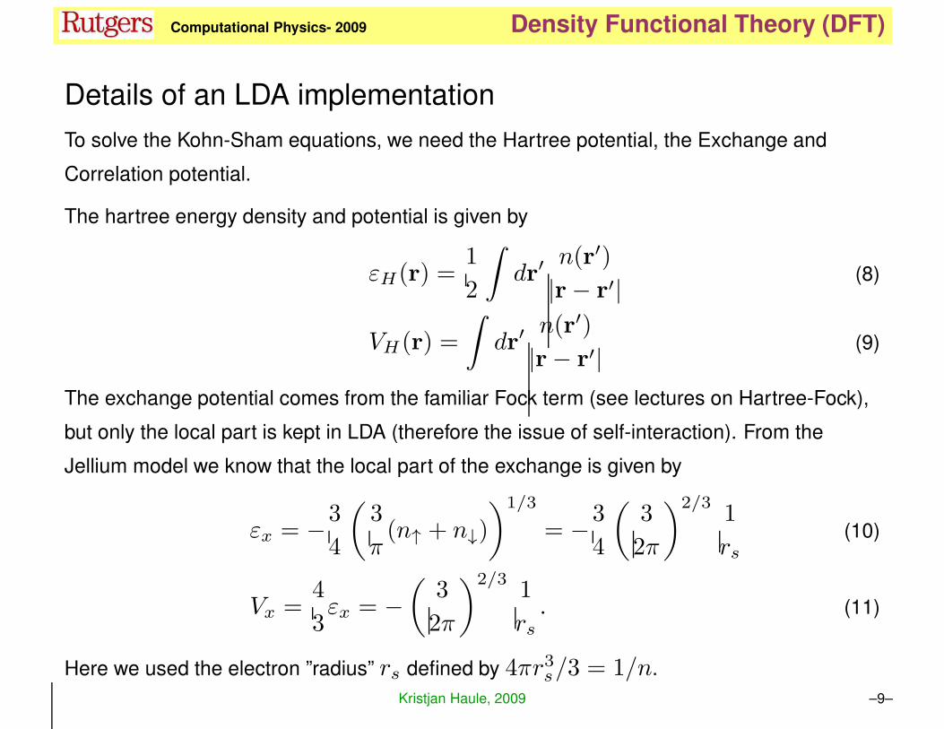
Details of an LDA implementation
To solve the Kohn-Sham equations, we need the Hartree potential, the Exchange and
Correlation potential.
The hartree energy density and potential is given by
εH(r) =1
2
∫
dr′n(r′)
|r− r′| (8)
VH(r) =
∫
dr′n(r′)
|r− r′| (9)
The exchange potential comes from the familiar Fock term (see lectures on Hartree-Fock),
but only the local part is kept in LDA (therefore the issue of self-interaction). From the
Jellium model we know that the local part of the exchange is given by
εx = −3
4
(
3
π(n↑ + n↓)
)1/3
= −3
4
(
3
2π
)2/31
rs(10)
Vx =4
3εx = −
(
3
2π
)2/31
rs. (11)
Here we used the electron ”radius” rs defined by 4πr3s/3 = 1/n.
Kristjan Haule, 2009 –9–
KH Computational Physics- 2009 Density Functional Theory (DFT)
The correlation potential can be expressed by the energy density. From Eq. (7) we see
Vc(r, σ) =δEc[n]
δn(r, σ)= εc[n(r)] + n(r)
δεc[n(r)]
δn(r, σ)(12)
The most accurate formulae for the exchange-corelation functional were obtained by fittingthe QMC results for the Jellium model. Various parametrizations are available. We will useone of the most popular choices due to Vosko-Wilk (PRB 22, 3812 (1980))
εc =A
2
{
log
(
x2
X(x)
)
+ 2b
Qarctan
(
Q
2x + b
)
−
bx0
X(x0)
[
log
(
(x − x0)2
X(x)
)
+2(b + 2x0)
Qarctan
(
Q
2x + b
)]}
(13)
with x =√rs, X(x) = x2 + bx+ c, and Q =
√4c− b2. Parameters are
A = 0.0621814, x0 = −0.10498, b = 3.72744 and c = 12.9352. Finally, the
potential is given by
Vc = εc −1
6A
c(x− x0)− bxx0(x− x0)(x2 + bx+ c)
. (14)
Kristjan Haule, 2009 –10–
KH Computational Physics- 2009 Density Functional Theory (DFT)
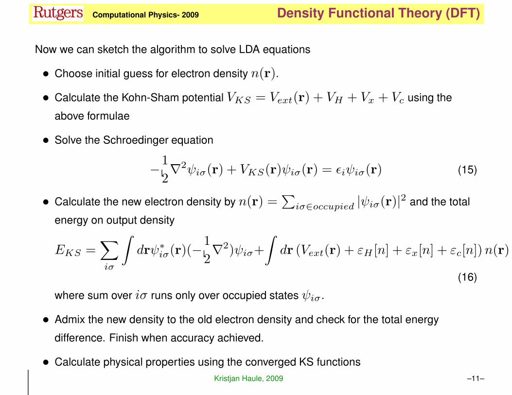
Now we can sketch the algorithm to solve LDA equations
• Choose initial guess for electron density n(r).
• Calculate the Kohn-Sham potential VKS = Vext(r) + VH + Vx + Vc using the
above formulae
• Solve the Schroedinger equation
−1
2∇2ψiσ(r) + VKS(r)ψiσ(r) = ǫiψiσ(r) (15)
• Calculate the new electron density by n(r) =∑
iσ∈occupied |ψiσ(r)|2 and the total
energy on output density
EKS =∑
iσ
∫
drψ∗iσ(r)(−
1
2∇2)ψiσ+
∫
dr (Vext(r) + εH [n] + εx[n] + εc[n])n(r)
(16)
where sum over iσ runs only over occupied states ψiσ .
• Admix the new density to the old electron density and check for the total energy
difference. Finish when accuracy achieved.
• Calculate physical properties using the converged KS functions
Kristjan Haule, 2009 –11–
KH Computational Physics- 2009 Density Functional Theory (DFT)
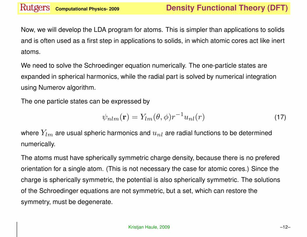
Now, we will develop the LDA program for atoms. This is simpler than applications to solids
and is often used as a first step in applications to solids, in which atomic cores act like inert
atoms.
We need to solve the Schroedinger equation numerically. The one-particle states are
expanded in spherical harmonics, while the radial part is solved by numerical integration
using Numerov algorithm.
The one particle states can be expressed by
ψnlm(r) = Ylm(θ, φ)r−1unl(r) (17)
where Ylm are usual spheric harmonics and unl are radial functions to be determined
numerically.
The atoms must have spherically symmetric charge density, because there is no prefered
orientation for a single atom. (This is not necessary the case for atomic cores.) Since the
charge is spherically symmetric, the potential is also spherically symmetric. The solutions
of the Schroedinger equations are not symmetric, but a set, which can restore the
symmetry, must be degenerate.
Kristjan Haule, 2009 –12–
KH Computational Physics- 2009 Density Functional Theory (DFT)
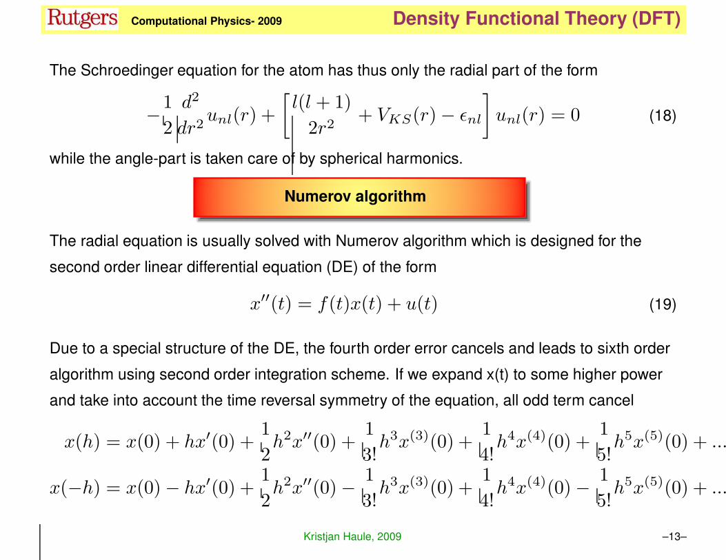
The Schroedinger equation for the atom has thus only the radial part of the form
−1
2
d2
dr2unl(r) +
[
l(l + 1)
2r2+ VKS(r)− ǫnl
]
unl(r) = 0 (18)
while the angle-part is taken care of by spherical harmonics.
Numerov algorithm
The radial equation is usually solved with Numerov algorithm which is designed for the
second order linear differential equation (DE) of the form
x′′(t) = f(t)x(t) + u(t) (19)
Due to a special structure of the DE, the fourth order error cancels and leads to sixth order
algorithm using second order integration scheme. If we expand x(t) to some higher power
and take into account the time reversal symmetry of the equation, all odd term cancel
x(h) = x(0) + hx′(0) +1
2h2x′′(0) +
1
3!h3x(3)(0) +
1
4!h4x(4)(0) +
1
5!h5x(5)(0) + ...
x(−h) = x(0)− hx′(0) +1
2h2x′′(0)− 1
3!h3x(3)(0) +
1
4!h4x(4)(0)− 1
5!h5x(5)(0) + ...
Kristjan Haule, 2009 –13–
KH Computational Physics- 2009 Density Functional Theory (DFT)
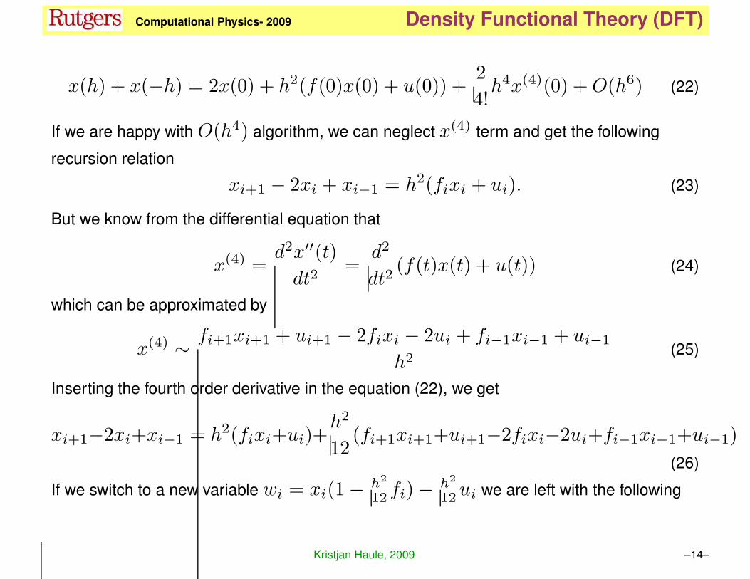
x(h) + x(−h) = 2x(0) + h2(f(0)x(0) + u(0)) +2
4!h4x(4)(0) +O(h6) (22)
If we are happy with O(h4) algorithm, we can neglect x(4) term and get the following
recursion relation
xi+1 − 2xi + xi−1 = h2(fixi + ui). (23)
But we know from the differential equation that
x(4) =d2x′′(t)
dt2=
d2
dt2(f(t)x(t) + u(t)) (24)
which can be approximated by
x(4) ∼ fi+1xi+1 + ui+1 − 2fixi − 2ui + fi−1xi−1 + ui−1
h2(25)
Inserting the fourth order derivative in the equation (22), we get
xi+1−2xi+xi−1 = h2(fixi+ui)+h2
12(fi+1xi+1+ui+1−2fixi−2ui+fi−1xi−1+ui−1)
(26)
If we switch to a new variable wi = xi(1− h2
12 fi)− h2
12ui we are left with the following
Kristjan Haule, 2009 –14–
KH Computational Physics- 2009 Density Functional Theory (DFT)
equation
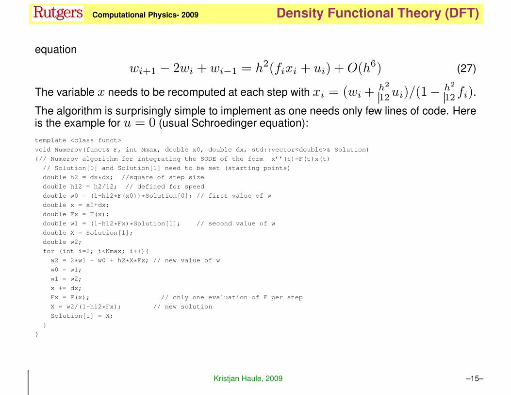
wi+1 − 2wi + wi−1 = h2(fixi + ui) +O(h6) (27)
The variable x needs to be recomputed at each step with xi = (wi+h2
12ui)/(1− h2
12 fi).
The algorithm is surprisingly simple to implement as one needs only few lines of code. Hereis the example for u = 0 (usual Schroedinger equation):
template <class funct>
void Numerov(funct& F, int Nmax, double x0, double dx, std::vector<double>& Solution)
{// Numerov algorithm for integrating the SODE of the form x’’(t)=F(t)x(t)
// Solution[0] and Solution[1] need to be set (starting points)
double h2 = dx*dx; //square of step size
double h12 = h2/12; // defined for speed
double w0 = (1-h12*F(x0))*Solution[0]; // first value of w
double x = x0+dx;
double Fx = F(x);
double w1 = (1-h12*Fx)*Solution[1]; // second value of w
double X = Solution[1];
double w2;
for (int i=2; i<Nmax; i++){
w2 = 2*w1 - w0 + h2*X*Fx; // new value of w
w0 = w1;
w1 = w2;
x += dx;
Fx = F(x); // only one evaluation of F per step
X = w2/(1-h12*Fx); // new solution
Solution[i] = X;
}
}
Kristjan Haule, 2009 –15–
KH Computational Physics- 2009 Density Functional Theory (DFT)
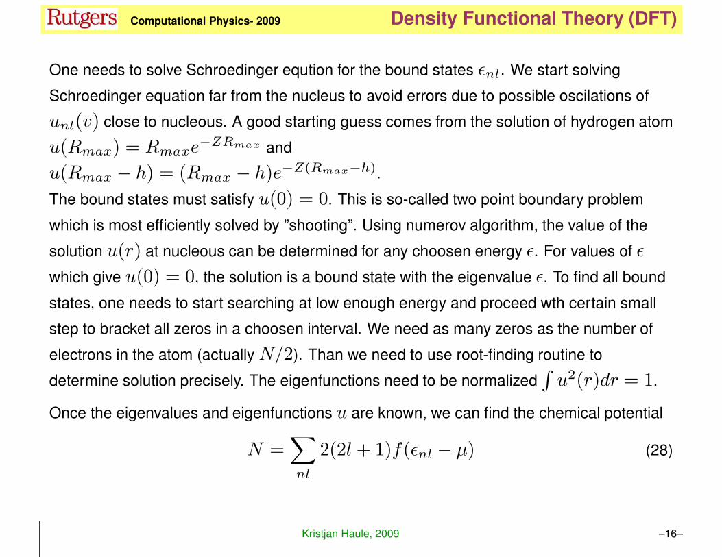
One needs to solve Schroedinger eqution for the bound states ǫnl. We start solving
Schroedinger equation far from the nucleus to avoid errors due to possible oscilations of
unl(v) close to nucleous. A good starting guess comes from the solution of hydrogen atom
u(Rmax) = Rmaxe−ZRmax and
u(Rmax − h) = (Rmax − h)e−Z(Rmax−h).
The bound states must satisfy u(0) = 0. This is so-called two point boundary problem
which is most efficiently solved by ”shooting”. Using numerov algorithm, the value of the
solution u(r) at nucleous can be determined for any choosen energy ǫ. For values of ǫ
which give u(0) = 0, the solution is a bound state with the eigenvalue ǫ. To find all bound
states, one needs to start searching at low enough energy and proceed wth certain small
step to bracket all zeros in a choosen interval. We need as many zeros as the number of
electrons in the atom (actually N/2). Than we need to use root-finding routine to
determine solution precisely. The eigenfunctions need to be normalized∫
u2(r)dr = 1.
Once the eigenvalues and eigenfunctions u are known, we can find the chemical potential
N =∑
nl
2(2l + 1)f(ǫnl − µ) (28)
Kristjan Haule, 2009 –16–
KH Computational Physics- 2009 Density Functional Theory (DFT)
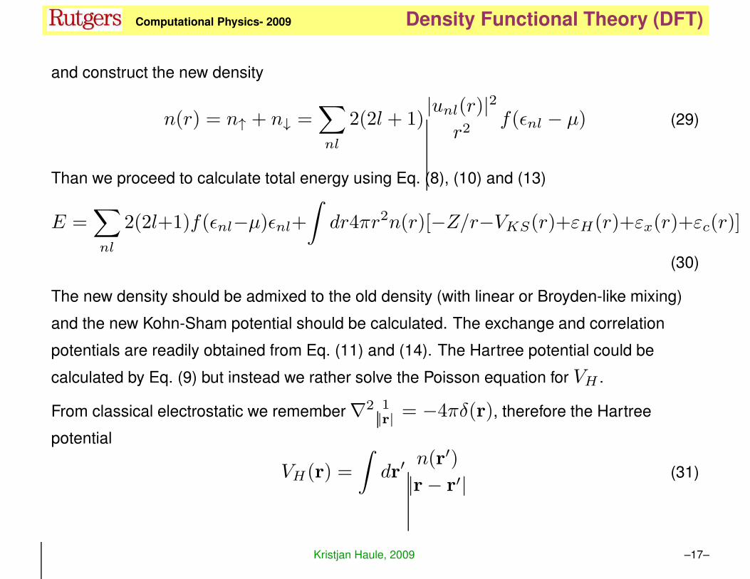
and construct the new density
n(r) = n↑ + n↓ =∑
nl
2(2l + 1)|unl(r)|2
r2f(ǫnl − µ) (29)
Than we proceed to calculate total energy using Eq. (8), (10) and (13)
E =∑
nl
2(2l+1)f(ǫnl−µ)ǫnl+∫
dr4πr2n(r)[−Z/r−VKS(r)+εH(r)+εx(r)+εc(r)]
(30)
The new density should be admixed to the old density (with linear or Broyden-like mixing)
and the new Kohn-Sham potential should be calculated. The exchange and correlation
potentials are readily obtained from Eq. (11) and (14). The Hartree potential could be
calculated by Eq. (9) but instead we rather solve the Poisson equation for VH .
From classical electrostatic we remember ∇2 1|r| = −4πδ(r), therefore the Hartree
potential
VH(r) =
∫
dr′n(r′)
|r− r′| (31)
Kristjan Haule, 2009 –17–
KH Computational Physics- 2009 Density Functional Theory (DFT)
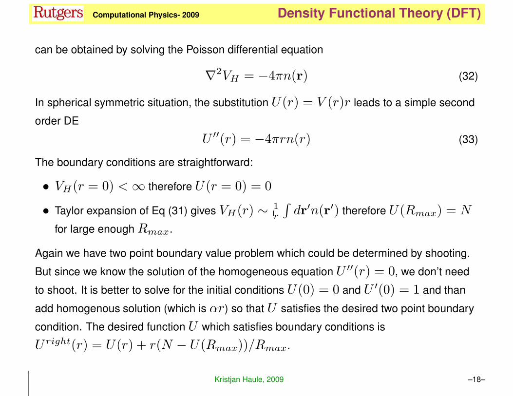
can be obtained by solving the Poisson differential equation
∇2VH = −4πn(r) (32)
In spherical symmetric situation, the substitution U(r) = V (r)r leads to a simple second
order DE
U ′′(r) = −4πrn(r) (33)
The boundary conditions are straightforward:
• VH(r = 0) <∞ therefore U(r = 0) = 0
• Taylor expansion of Eq (31) gives VH(r) ∼ 1r
∫
dr′n(r′) therefore U(Rmax) = N
for large enoughRmax.
Again we have two point boundary value problem which could be determined by shooting.
But since we know the solution of the homogeneous equation U ′′(r) = 0, we don’t need
to shoot. It is better to solve for the initial conditions U(0) = 0 and U ′(0) = 1 and than
add homogenous solution (which is αr) so that U satisfies the desired two point boundary
condition. The desired function U which satisfies boundary conditions is
U right(r) = U(r) + r(N − U(Rmax))/Rmax.
Kristjan Haule, 2009 –18–
KH Computational Physics- 2009 Density Functional Theory (DFT)
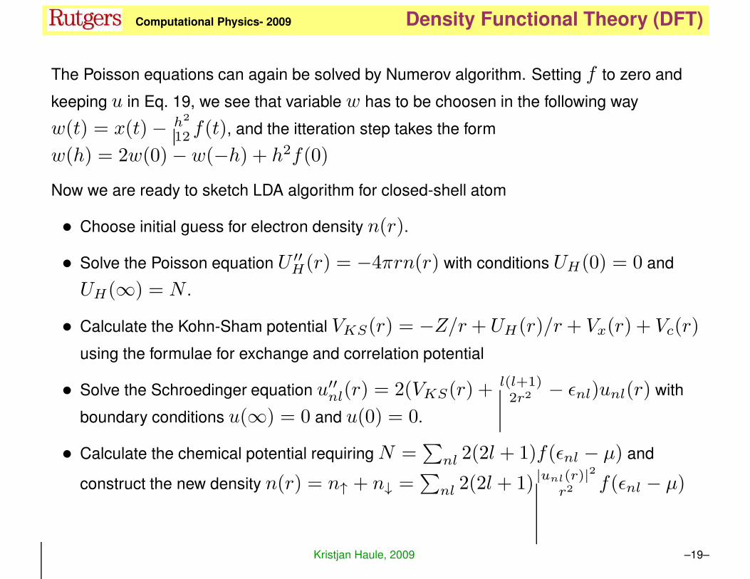
The Poisson equations can again be solved by Numerov algorithm. Setting f to zero and
keeping u in Eq. 19, we see that variable w has to be choosen in the following way
w(t) = x(t)− h2
12 f(t), and the itteration step takes the form
w(h) = 2w(0)− w(−h) + h2f(0)
Now we are ready to sketch LDA algorithm for closed-shell atom
• Choose initial guess for electron density n(r).
• Solve the Poisson equation U ′′H(r) = −4πrn(r) with conditions UH(0) = 0 and
UH(∞) = N .
• Calculate the Kohn-Sham potential VKS(r) = −Z/r +UH(r)/r+ Vx(r) + Vc(r)
using the formulae for exchange and correlation potential
• Solve the Schroedinger equation u′′nl(r) = 2(VKS(r) +l(l+1)2r2 − ǫnl)unl(r) with
boundary conditions u(∞) = 0 and u(0) = 0.
• Calculate the chemical potential requiringN =∑
nl 2(2l + 1)f(ǫnl − µ) and
construct the new density n(r) = n↑ + n↓ =∑
nl 2(2l + 1) |unl(r)|2
r2 f(ǫnl − µ)
Kristjan Haule, 2009 –19–
KH Computational Physics- 2009 Density Functional Theory (DFT)
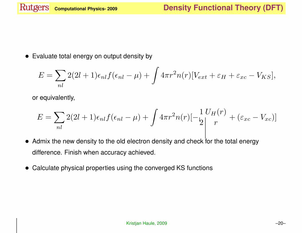
• Evaluate total energy on output density by
E =∑
nl
2(2l + 1)ǫnlf(ǫnl − µ) +
∫
4πr2n(r)[Vext + εH + εxc − VKS ],
or equivalently,
E =∑
nl
2(2l + 1)ǫnlf(ǫnl − µ) +
∫
4πr2n(r)[−1
2
UH(r)
r+ (εxc − Vxc)]
• Admix the new density to the old electron density and check for the total energy
difference. Finish when accuracy achieved.
• Calculate physical properties using the converged KS functions
Kristjan Haule, 2009 –20–
KH Computational Physics- 2009 Density Functional Theory (DFT)
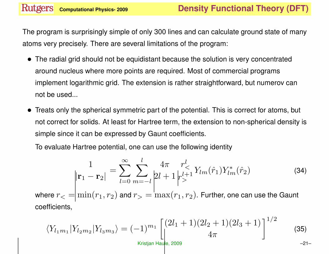
The program is surprisingly simple of only 300 lines and can calculate ground state of many
atoms very precisely. There are several limitations of the program:
• The radial grid should not be equidistant because the solution is very concentrated
around nucleus where more points are required. Most of commercial programs
implement logarithmic grid. The extension is rather straightforward, but numerov can
not be used...
• Treats only the spherical symmetric part of the potential. This is correct for atoms, but
not correct for solids. At least for Hartree term, the extension to non-spherical density is
simple since it can be expressed by Gaunt coefficients.
To evaluate Hartree potential, one can use the following identity
1
|r1 − r2|=
∞∑
l=0
l∑
m=−l
4π
2l + 1
rl<rl+1>
Ylm(r1)Y∗lm(r2) (34)
where r< = min(r1, r2) and r> = max(r1, r2). Further, one can use the Gaunt
coefficients,
〈Yl1m1 |Yl2m2 |Yl3m3〉 = (−1)m1
[
(2l1 + 1)(2l2 + 1)(2l3 + 1)
4π
]1/2
(35)
Kristjan Haule, 2009 –21–
KH Computational Physics- 2009 Density Functional Theory (DFT)
×
l1 l2 l3
0 0 0
l1 l2 l3
−m1 m2 m3
(36)
They can be evaluated using 3j symbols which are given standard textbooks on angular
momentum (Racah formulas).
The precision of the results are however suprisingly good. We will compare them to
published results at
http://physics.nist.gov/PhysRefData/DFTdata/Tables/ptable.html
Using 10000 radial points with maximum radius 10 and dr=0.001 (which needs few second
on PC for any atom), we get for He total energy E=-2.834836 Hartree which is the same as
the published results. The kinetic energy is also the same 2.767922 Hartree.
The more complicated example is Krypton with 36 electrons and therefore filled shell. We
get E=-2750.1453 while the published results is E=-2750.147940. The results can be
improved by taking more dense mesh or implement logarithmic mesh.
Finally, we can test how good this approximatio is for open shell atoms (with partially filled
shells). Lets take C as an example. Its electronic configuration is C : [He]2s22p2. The
two outer p electrons should fill the Hund’s coupling and should align in the same directionKristjan Haule, 2009 –22–
KH Computational Physics- 2009 Density Functional Theory (DFT)
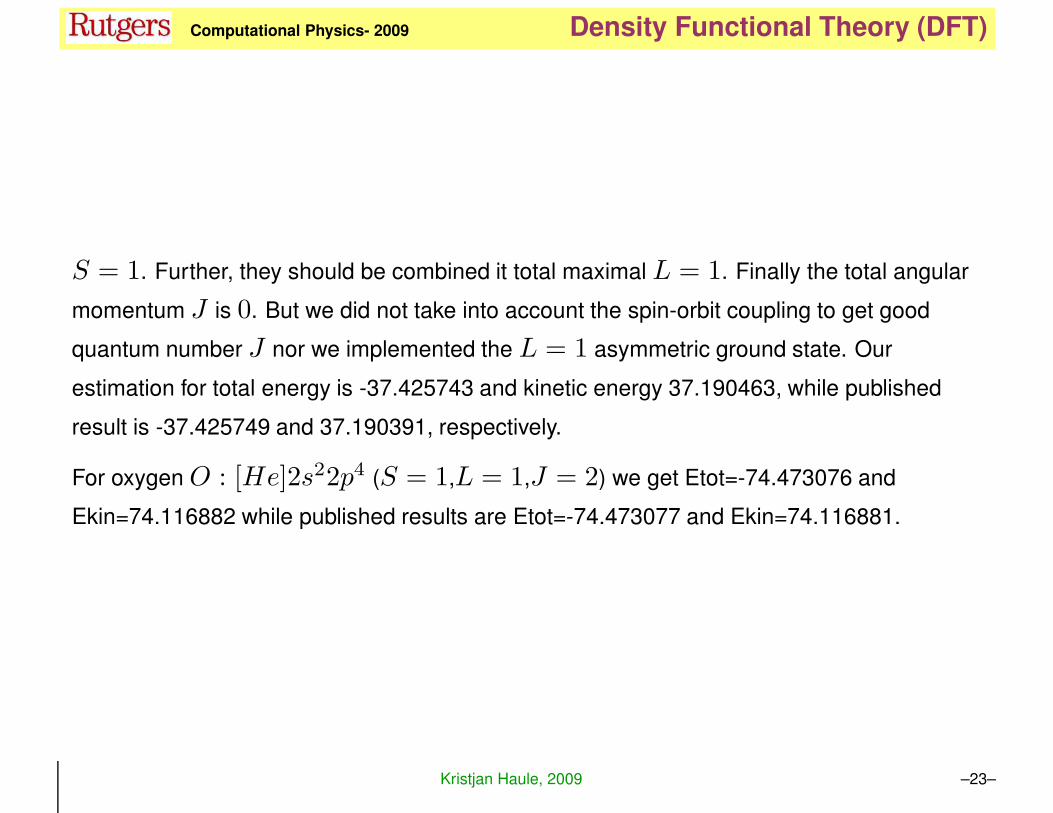
S = 1. Further, they should be combined it total maximal L = 1. Finally the total angular
momentum J is 0. But we did not take into account the spin-orbit coupling to get good
quantum number J nor we implemented the L = 1 asymmetric ground state. Our
estimation for total energy is -37.425743 and kinetic energy 37.190463, while published
result is -37.425749 and 37.190391, respectively.
For oxygenO : [He]2s22p4 (S = 1,L = 1,J = 2) we get Etot=-74.473076 and
Ekin=74.116882 while published results are Etot=-74.473077 and Ekin=74.116881.
Kristjan Haule, 2009 –23–
KH Computational Physics- 2009 Density Functional Theory (DFT)
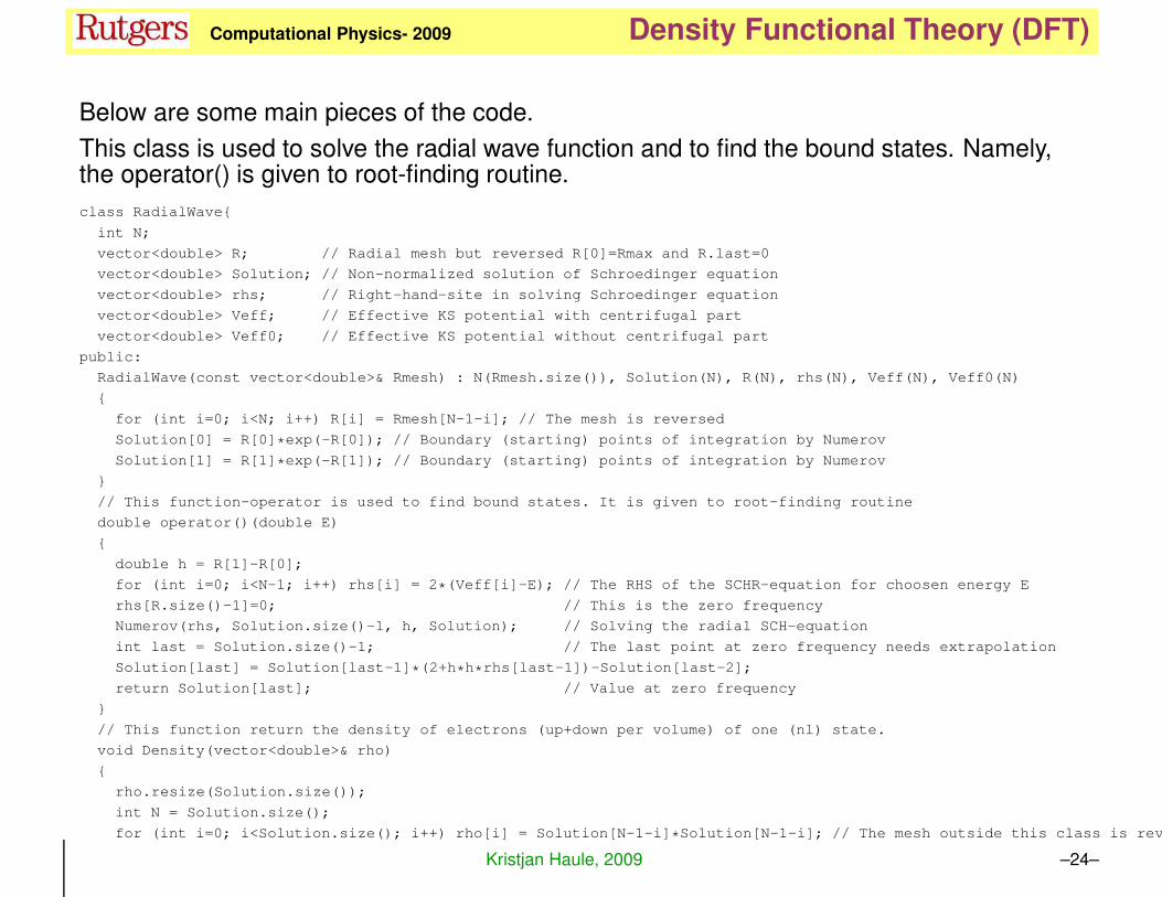
Below are some main pieces of the code.
This class is used to solve the radial wave function and to find the bound states. Namely,the operator() is given to root-finding routine.
class RadialWave{
int N;
vector<double> R; // Radial mesh but reversed R[0]=Rmax and R.last=0
vector<double> Solution; // Non-normalized solution of Schroedinger equation
vector<double> rhs; // Right-hand-site in solving Schroedinger equation
vector<double> Veff; // Effective KS potential with centrifugal part
vector<double> Veff0; // Effective KS potential without centrifugal part
public:
RadialWave(const vector<double>& Rmesh) : N(Rmesh.size()), Solution(N), R(N), rhs(N), Veff(N), Veff0(N)
{
for (int i=0; i<N; i++) R[i] = Rmesh[N-1-i]; // The mesh is reversed
Solution[0] = R[0]*exp(-R[0]); // Boundary (starting) points of integration by Numerov
Solution[1] = R[1]*exp(-R[1]); // Boundary (starting) points of integration by Numerov
}
// This function-operator is used to find bound states. It is given to root-finding routine
double operator()(double E)
{
double h = R[1]-R[0];
for (int i=0; i<N-1; i++) rhs[i] = 2*(Veff[i]-E); // The RHS of the SCHR-equation for choosen energy E
rhs[R.size()-1]=0; // This is the zero frequency
Numerov(rhs, Solution.size()-1, h, Solution); // Solving the radial SCH-equation
int last = Solution.size()-1; // The last point at zero frequency needs extrapolation
Solution[last] = Solution[last-1]*(2+h*h*rhs[last-1])-Solution[last-2];
return Solution[last]; // Value at zero frequency
}
// This function return the density of electrons (up+down per volume) of one (nl) state.
void Density(vector<double>& rho)
{
rho.resize(Solution.size());
int N = Solution.size();
for (int i=0; i<Solution.size(); i++) rho[i] = Solution[N-1-i]*Solution[N-1-i]; // The mesh outside this class is reversed!
Kristjan Haule, 2009 –24–
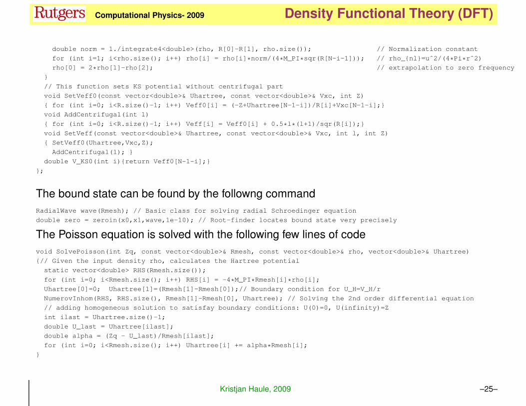
KH Computational Physics- 2009 Density Functional Theory (DFT)
double norm = 1./integrate4<double>(rho, R[0]-R[1], rho.size()); // Normalization constant
for (int i=1; i<rho.size(); i++) rho[i] = rho[i]*norm/(4*M_PI*sqr(R[N-i-1])); // rho_{nl}=uˆ2/(4*Pi*rˆ2)
rho[0] = 2*rho[1]-rho[2]; // extrapolation to zero frequency
}
// This function sets KS potential without centrifugal part
void SetVeff0(const vector<double>& Uhartree, const vector<double>& Vxc, int Z)
{ for (int i=0; i<R.size()-1; i++) Veff0[i] = (-Z+Uhartree[N-1-i])/R[i]+Vxc[N-1-i];}
void AddCentrifugal(int l)
{ for (int i=0; i<R.size()-1; i++) Veff[i] = Veff0[i] + 0.5*l*(l+1)/sqr(R[i]);}
void SetVeff(const vector<double>& Uhartree, const vector<double>& Vxc, int l, int Z)
{ SetVeff0(Uhartree,Vxc,Z);
AddCentrifugal(l); }
double V_KS0(int i){return Veff0[N-1-i];}
};
The bound state can be found by the followng command
RadialWave wave(Rmesh); // Basic class for solving radial Schroedinger equation
double zero = zeroin(x0,x1,wave,1e-10); // Root-finder locates bound state very precisely
The Poisson equation is solved with the following few lines of code
void SolvePoisson(int Zq, const vector<double>& Rmesh, const vector<double>& rho, vector<double>& Uhartree)
{// Given the input density rho, calculates the Hartree potential
static vector<double> RHS(Rmesh.size());
for (int i=0; i<Rmesh.size(); i++) RHS[i] = -4*M_PI*Rmesh[i]*rho[i];
Uhartree[0]=0; Uhartree[1]=(Rmesh[1]-Rmesh[0]);// Boundary condition for U_H=V_H/r
NumerovInhom(RHS, RHS.size(), Rmesh[1]-Rmesh[0], Uhartree); // Solving the 2nd order differential equation
// adding homogeneous solution to satisfay boundary conditions: U(0)=0, U(infinity)=Z
int ilast = Uhartree.size()-1;
double U_last = Uhartree[ilast];
double alpha = (Zq - U_last)/Rmesh[ilast];
for (int i=0; i<Rmesh.size(); i++) Uhartree[i] += alpha*Rmesh[i];
}
Kristjan Haule, 2009 –25–
KH Computational Physics- 2009 Density Functional Theory (DFT)
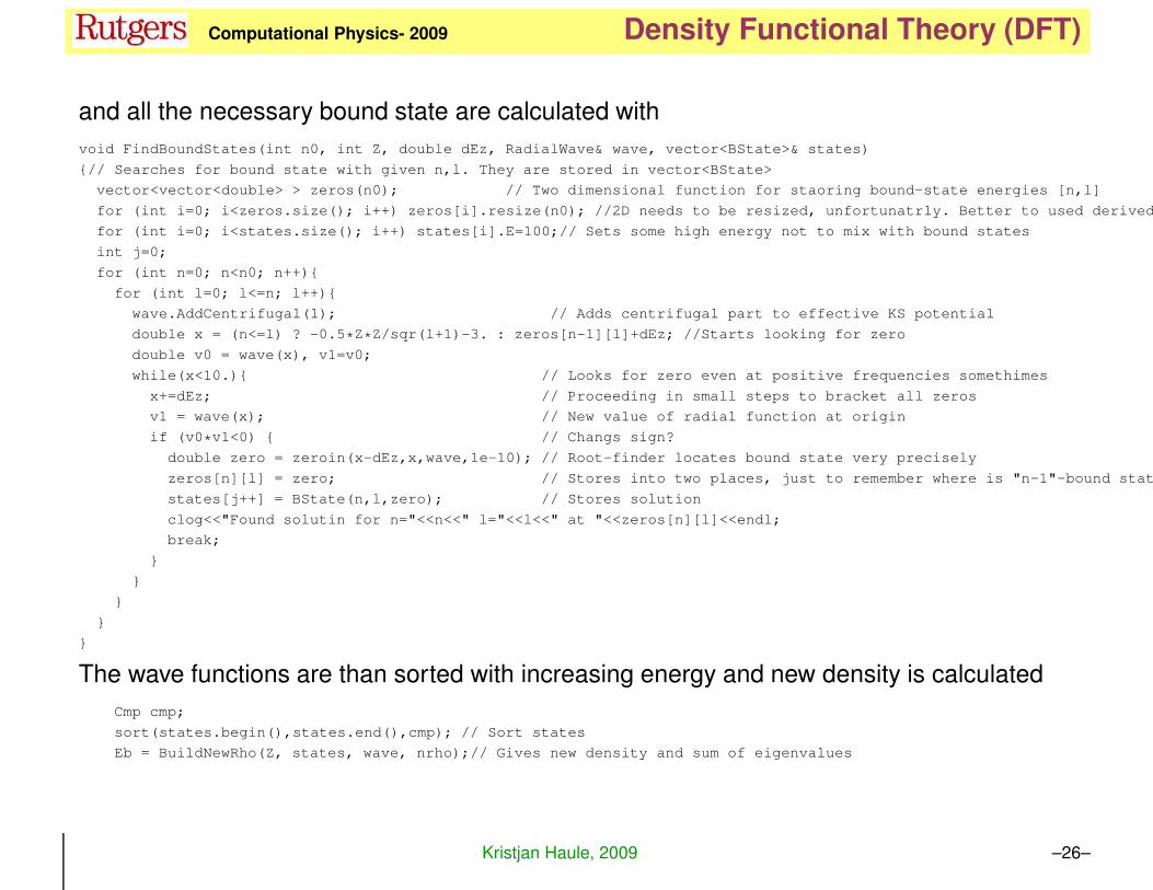
and all the necessary bound state are calculated with
void FindBoundStates(int n0, int Z, double dEz, RadialWave& wave, vector<BState>& states)
{// Searches for bound state with given n,l. They are stored in vector<BState>
vector<vector<double> > zeros(n0); // Two dimensional function for staoring bound-state energies [n,l]
for (int i=0; i<zeros.size(); i++) zeros[i].resize(n0); //2D needs to be resized, unfortunatrly. Better to used derived
for (int i=0; i<states.size(); i++) states[i].E=100;// Sets some high energy not to mix with bound states
int j=0;
for (int n=0; n<n0; n++){
for (int l=0; l<=n; l++){
wave.AddCentrifugal(l); // Adds centrifugal part to effective KS potential
double x = (n<=l) ? -0.5*Z*Z/sqr(l+1)-3. : zeros[n-1][l]+dEz; //Starts looking for zero
double v0 = wave(x), v1=v0;
while(x<10.){ // Looks for zero even at positive frequencies somethimes
x+=dEz; // Proceeding in small steps to bracket all zeros
v1 = wave(x); // New value of radial function at origin
if (v0*v1<0) { // Changs sign?
double zero = zeroin(x-dEz,x,wave,1e-10); // Root-finder locates bound state very precisely
zeros[n][l] = zero; // Stores into two places, just to remember where is "n-1"-bound state
states[j++] = BState(n,l,zero); // Stores solution
clog<<"Found solutin for n="<<n<<" l="<<l<<" at "<<zeros[n][l]<<endl;
break;
}
}
}
}
}
The wave functions are than sorted with increasing energy and new density is calculated
Cmp cmp;
sort(states.begin(),states.end(),cmp); // Sort states
Eb = BuildNewRho(Z, states, wave, nrho);// Gives new density and sum of eigenvalues
Kristjan Haule, 2009 –26–
KH Computational Physics- 2009 Density Functional Theory (DFT)
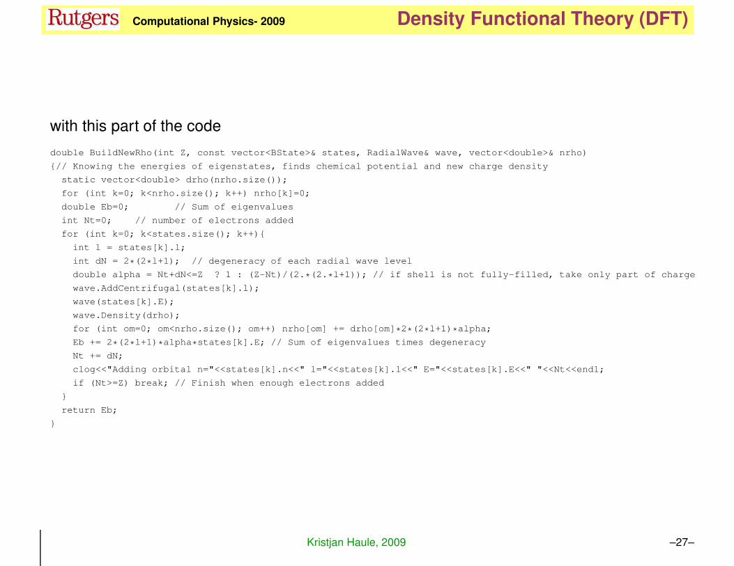
with this part of the code
double BuildNewRho(int Z, const vector<BState>& states, RadialWave& wave, vector<double>& nrho)
{// Knowing the energies of eigenstates, finds chemical potential and new charge density
static vector<double> drho(nrho.size());
for (int k=0; k<nrho.size(); k++) nrho[k]=0;
double Eb=0; // Sum of eigenvalues
int Nt=0; // number of electrons added
for (int k=0; k<states.size(); k++){
int l = states[k].l;
int dN = 2*(2*l+1); // degeneracy of each radial wave level
double alpha = Nt+dN<=Z ? 1 : (Z-Nt)/(2.*(2.*l+1)); // if shell is not fully-filled, take only part of charge
wave.AddCentrifugal(states[k].l);
wave(states[k].E);
wave.Density(drho);
for (int om=0; om<nrho.size(); om++) nrho[om] += drho[om]*2*(2*l+1)*alpha;
Eb += 2*(2*l+1)*alpha*states[k].E; // Sum of eigenvalues times degeneracy
Nt += dN;
clog<<"Adding orbital n="<<states[k].n<<" l="<<states[k].l<<" E="<<states[k].E<<" "<<Nt<<endl;
if (Nt>=Z) break; // Finish when enough electrons added
}
return Eb;
}
Kristjan Haule, 2009 –27–
KH Computational Physics- 2009 Density Functional Theory (DFT)
Results of LDA calculation
• LDA was intended for systems with slowly varying electronic density. Should fail for real
materials.
• But: LDA is applied to all kind of systems and in general, LDA calculations lead to very
good agreement with experiment, except for strongly correlated materials (with open f
and sometimes d shells).
• Geometries
– The accuracy of geometry is better than 0.1A
– Lattice constants are obtained within 4% or better.
• Energies
– Accuracy for energies usually better than 0.2eV/atom in special cases even better
than 0.01 eV/atom. (Factor of 2 worse than best quantum chemical calculations).
– Atomization energies in simple molecules: up to 4kcal/mol (≈ 0.2eV/atom)
Kristjan Haule, 2009 –28–
KH Computational Physics- 2009 Density Functional Theory (DFT)
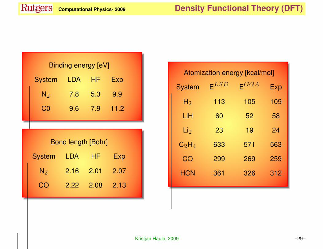
Binding energy [eV]
System LDA HF Exp
N2 7.8 5.3 9.9
C0 9.6 7.9 11.2
Bond length [Bohr]
System LDA HF Exp
N2 2.16 2.01 2.07
CO 2.22 2.08 2.13
Atomization energy [kcal/mol]
System ELSD EGGA Exp
H2 113 105 109
LiH 60 52 58
Li2 23 19 24
C2H4 633 571 563
CO 299 269 259
HCN 361 326 312
Kristjan Haule, 2009 –29–
KH Computational Physics- 2009 Density Functional Theory (DFT)
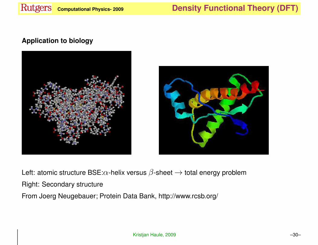
Application to biology
Left: atomic structure BSE:α-helix versus β-sheet → total energy problem
Right: Secondary structure
From Joerg Neugebauer; Protein Data Bank, http://www.rcsb.org/
Kristjan Haule, 2009 –30–
KH Computational Physics- 2009 Density Functional Theory (DFT)
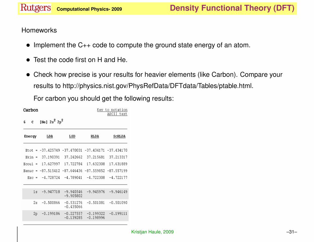
Homeworks
• Implement the C++ code to compute the ground state energy of an atom.
• Test the code first on H and He.
• Check how precise is your results for heavier elements (like Carbon). Compare your
results to http://physics.nist.gov/PhysRefData/DFTdata/Tables/ptable.html.
For carbon you should get the following results:
Kristjan Haule, 2009 –31–
KH Computational Physics- 2009 Density Functional Theory (DFT)
• (optional) : Implement one of the above mentioned extensions
– logarithmic radial grid (see details in Richard M. Martin’s book and at
http://physics.nist.gov/PhysRefData/DFTdata/radialgrids.html).
– breaking the spin symmetry (check the original articles how correlation energy and
potential change)
– breaking of spheric symmetry (only for Hartree term but not for XC term. The
implementation should be through gaunt coefficients- see again Richard M. Martin
or any web page on gaunt coefficients).
Kristjan Haule, 2009 –32–