Deep Mixtures of Factor Analysers

Yichuan Tang, Ruslan Salakhutdinov, Geoffrey Hinton

Presenter: Jianbo Yang

Duke University

September 6, 2012

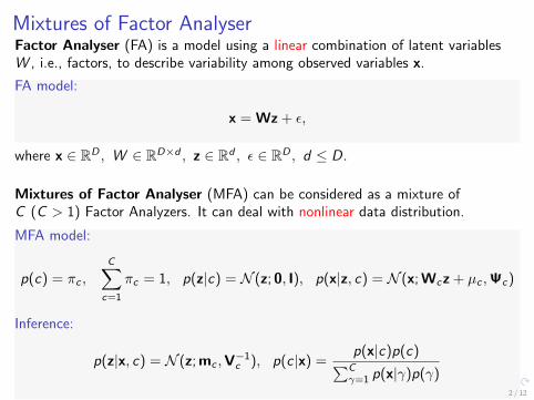
Mixtures of Factor AnalyserFactor Analyser (FA) is a model using a linear combination of latent variablesW , i.e., factors, to describe variability among observed variables x.

FA model:

x = Wz + ε,

where x ∈ RD , W ∈ RD×d , z ∈ Rd , ε ∈ RD , d ≤ D.

Mixtures of Factor Analyser (MFA) can be considered as a mixture ofC (C > 1) Factor Analyzers. It can deal with nonlinear data distribution.

MFA model:

p(c) = πc ,

C∑c=1

πc = 1, p(z|c) = N (z; 0, I), p(x|z, c) = N (x; Wcz + µc ,Ψc)

Inference:

p(z|x, c) = N (z; mc ,V−1c ), p(c |x) =

p(x|c)p(c)∑Cγ=1 p(x|γ)p(γ)

2 / 12

Improvements on MFA

Naive Way.Increase the mixture components or the factors dimension of per component.

Comments:1. Overfitting results in, particularly when modeling high-dimensional data.2. Chen et al (2010) have used Dirichlet process and Beta-Bernoulli processto infer these two variables respectively.

Sophisticated Way.Change p(z|c) = N (z; 0, I) to be p(z |c) = MFA(θc) , where θc is the MFAparameters for component c .

WHY? Ideally, aggregated posterior 1N

∑Nn=1 p(zn, cn = c |xn) is isotropic

Gaussian, but, in practice, it is not Gaussian.

3 / 12

Deep Mixtures of Factor Analysers

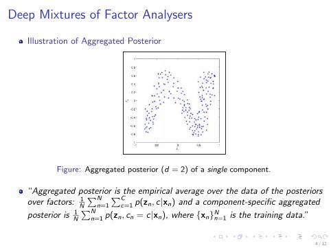
Illustration of Aggregated Posterior

Figure: Aggregated posterior (d = 2) of a single component.

“Aggregated posterior is the empirical average over the data of the posteriorsover factors: 1

N

∑Nn=1

∑Cc=1 p(zn, c |xn) and a component-specific aggregated

posterior is 1N

∑Nn=1 p(zn, cn = c |xn), where {xn}Nn=1 is the training data.”

4 / 12

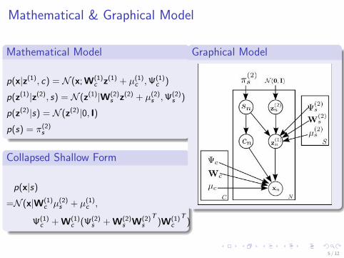
Mathematical & Graphical Model

Mathematical Model

p(x|z(1), c) = N (x; W(1)c z(1) + µ(1)

c ,Ψ(1)c )

p(z(1)|z(2), s) = N (z(1)|W(2)s z(2) + µ(2)

s ,Ψ(2)s )

p(z(2)|s) = N (z(2)|0, I)p(s) = π(2)

s

Collapsed Shallow Form

p(x|s)

=N (x|W(1)c µ(2)

s + µ(1)c ,

Ψ(1)c + W(1)

c (Ψ(2)s + W(2)

s W(2)s

T)W(1)

c

T)

Graphical Model

5 / 12

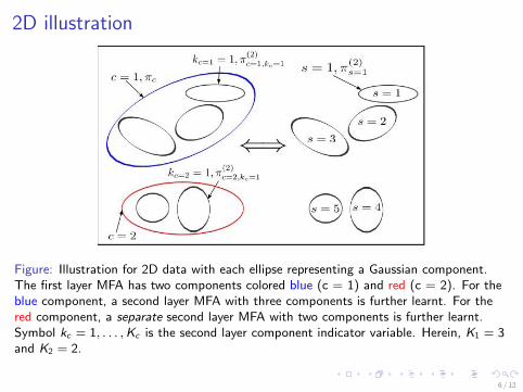
2D illustration

Figure: Illustration for 2D data with each ellipse representing a Gaussian component.The first layer MFA has two components colored blue (c = 1) and red (c = 2). For theblue component, a second layer MFA with three components is further learnt. For thered component, a separate second layer MFA with two components is further learnt.Symbol kc = 1, . . . ,Kc is the second layer component indicator variable. Herein, K1 = 3and K2 = 2.

6 / 12

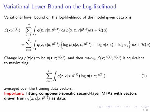
Variational Lower Bound on the Log-likelihood

Variational lower bound on the log-likelihood of the model given data x is

L(x; θ(1)) =C∑

c=1

∫z

q(z, c |x, θ(1)) log p(x, z, c |θ(1))dz +H(q)

=C∑

c=1

∫z

q(z, c |x; θ(1)){

log p(x|z, c ; θ(1)) + log p(z|c) + log πc}

dz +H(q)

Change log p(z|c) to be p(z|c ; θ(2)), and then maxθ(2) L(x; θ(1), θ(2)) is equivalentto maximizing

C∑c=1

∫z

q(z, c |x, θ(1)) log p(z|c ; θ(2)) (1)

averaged over the training data vectors.Important: fitting component-specific second-layer MFAs with vectorsdrawn from q(z, c |x, θ(1)) as data.

7 / 12

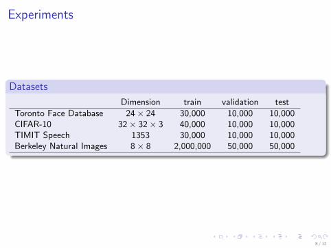
Experiments

Datasets

Dimension train validation testToronto Face Database 24× 24 30,000 10,000 10,000CIFAR-10 32× 32× 3 40,000 10,000 10,000TIMIT Speech 1353 30,000 10,000 10,000Berkeley Natural Images 8× 8 2,000,000 50,000 50,000

8 / 12

Overfitting for shallow MFA

Setting

1-layer MFA with 20 components (Iter 1 — 33)

2-layer MFA with 5 components for each of the first layer component (Iter 34— 53)

2-layer MFA is collapsed into a shallow MFA (Iter 34 — 53)

9 / 12

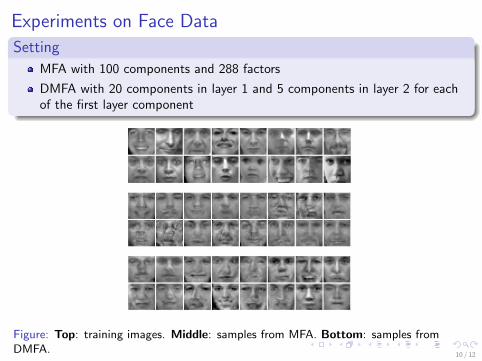
Experiments on Face Data

Setting

MFA with 100 components and 288 factors

DMFA with 20 components in layer 1 and 5 components in layer 2 for eachof the first layer component

Figure: Top: training images. Middle: samples from MFA. Bottom: samples fromDMFA.

10 / 12

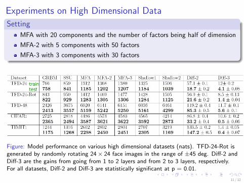
Experiments on High Dimensional Data

Setting

MFA with 20 components and the number of factors being half of dimension

MFA-2 with 5 components with 50 factors

MFA-3 with 3 components with 30 factors

Figure: Model performance on various high dimensional datasets (nats). TFD-24-Rot isgenerated by randomly rotating 24 × 24 face images in the range of ±45 deg. Diff-2 andDiff-3 are the gains from going from 1 to 2 layers and from 2 to 3 layers, respectively.For all datasets, Diff-2 and Diff-3 are statistically significant at p = 0.01.

11 / 12

Conclusions

An efficient way to learn deep density models is to greedily learn one layer ata time using one layer latent variable models.

Mixtures of Factor Analysers can be stacked to form Deep Mixtures of FactorAnalysers.

For each MFA component, the often non-Gaussian aggregated posterior isreplaced with a better prior, improving a variational lower bound on thetraining data.

DMFAs share lower-level factor loadings among higher-level MFAs, reducingoverfitting.

12 / 12