Decision Trees - Donald Bren School of Information and ...xhx/courses/CS273P/08-dectree-273p.pdf ·...
30
Decision Trees PROF XIAOHUI XIE SPRING 2019 CS 273P Machine Learning and Data Mining Slides courtesy of Alex Ihler
Transcript of Decision Trees - Donald Bren School of Information and ...xhx/courses/CS273P/08-dectree-273p.pdf ·...
Decision Trees
PROF XIAOHUI XIESPRING 2019
CS 273P Machine Learning and Data Mining
Slides courtesy of Alex Ihler

Decision trees• Functional form f(x;θ): nested “if-then-else” statements
– Discrete features: fully expressive (any function)
• Structure:– Internal nodes: check feature, branch on value
– Leaf nodes: output prediction
x1 x2 y0 0 1
0 1 -1
1 0 -1
1 1 1
“XOR” X1?
X2? X2?
if X1: # branch on feature at root if X2: return +1 # if true, branch on right child feature else: return -1 # & return leaf valueelse: # left branch: if X2: return -1 # branch on left child feature else: return +1 # & return leaf value
Parameters? Tree structure, features, and leaf outputs
0 0.1
0.2
0.3
0.4
0.5
0.6
0.7
0.8
0.9
10
0.1
0.2
0.3
0.4
0.5
0.6
0.7
0.8
0.9
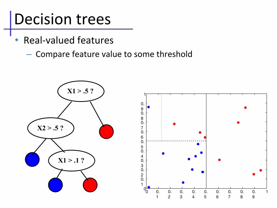
1X1 > .5 ?
X2 > .5 ?
X1 > .1 ?
Decision trees• Real-valued features
– Compare feature value to some threshold
X1 = ?
AB C D
X1 = ?
{A}{B,C,D}
X1 = ?
{A,D}{B,C}
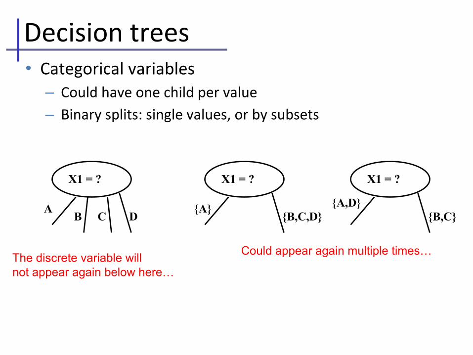
The discrete variable will not appear again below here…
Could appear again multiple times…
Decision trees• Categorical variables
– Could have one child per value
– Binary splits: single values, or by subsets
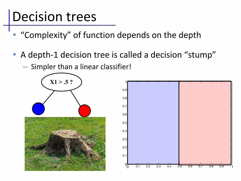
• “Complexity” of function depends on the depth
• A depth-1 decision tree is called a decision “stump”– Simpler than a linear classifier!
0 0.1 0.2 0.3 0.4 0.5 0.6 0.7 0.8 0.9 10
0.1
0.2
0.3
0.4
0.5
0.6
0.7
0.8
0.9
1X1 > .5 ?
Decision trees
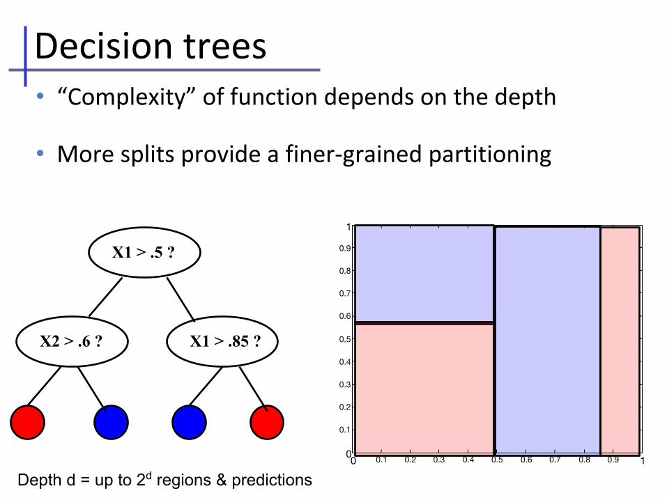
• “Complexity” of function depends on the depth
• More splits provide a finer-grained partitioning
0 0.1 0.2 0.3 0.4 0.5 0.6 0.7 0.8 0.9 10
0.1
0.2
0.3
0.4
0.5
0.6
0.7
0.8
0.9
1
X1 > .5 ?
X2 > .6 ? X1 > .85 ?
Depth d = up to 2d regions & predictions
Decision trees
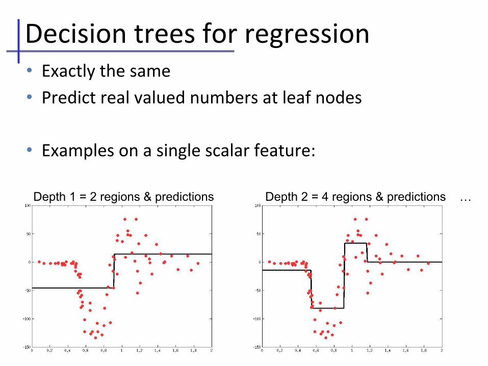
• Exactly the same
• Predict real valued numbers at leaf nodes
• Examples on a single scalar feature:
Depth 1 = 2 regions & predictions Depth 2 = 4 regions & predictions …
Decision trees for regression
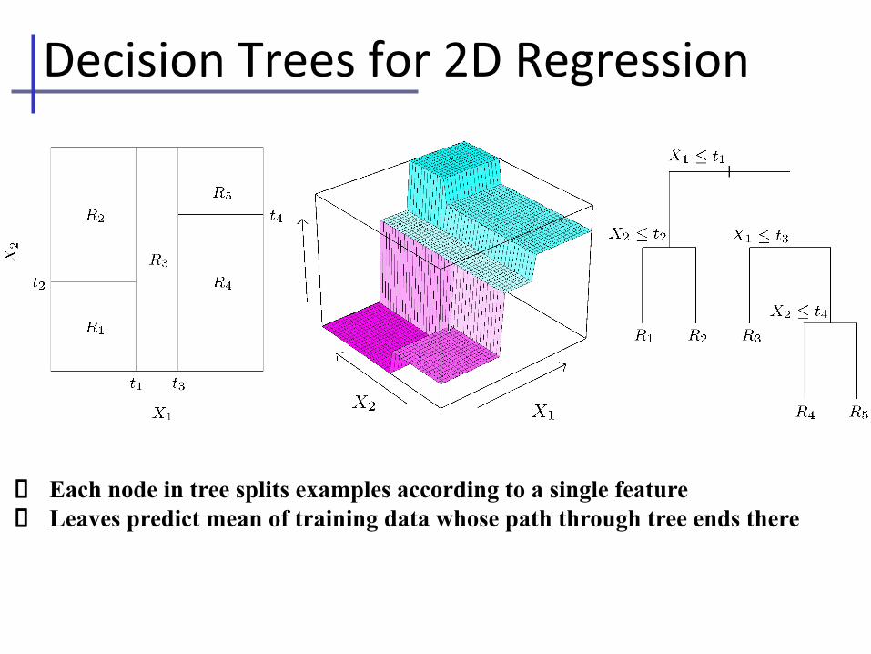
Decision Trees for 2D Regression
Each node in tree splits examples according to a single featureLeaves predict mean of training data whose path through tree ends there
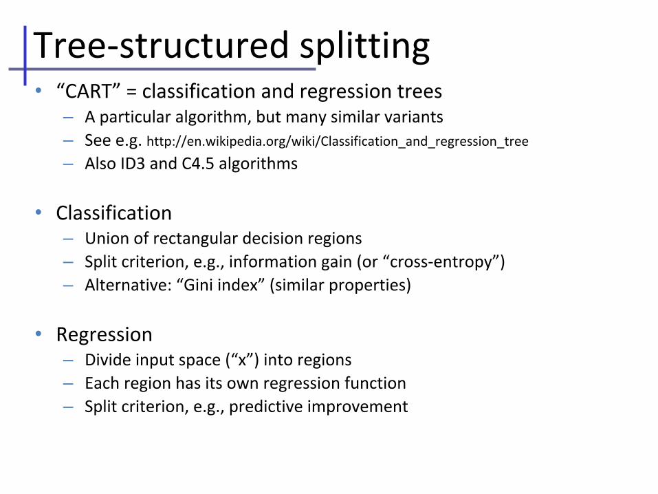
Tree-structured splitting• “CART” = classification and regression trees
– A particular algorithm, but many similar variants– See e.g. http://en.wikipedia.org/wiki/Classification_and_regression_tree
– Also ID3 and C4.5 algorithms
• Classification– Union of rectangular decision regions– Split criterion, e.g., information gain (or “cross-entropy”)– Alternative: “Gini index” (similar properties)
• Regression– Divide input space (“x”) into regions– Each region has its own regression function– Split criterion, e.g., predictive improvement
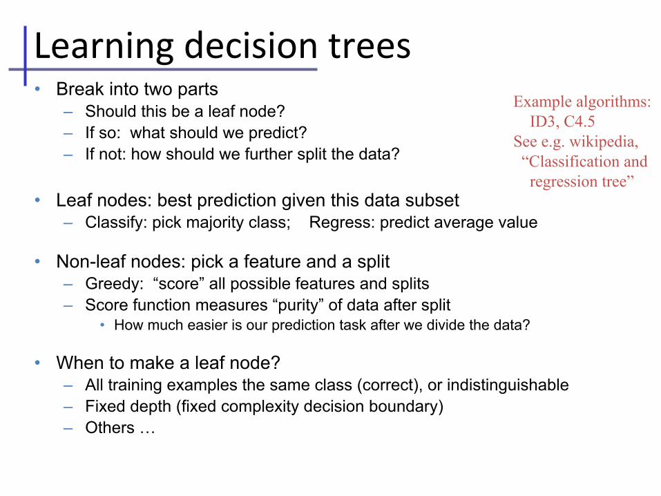
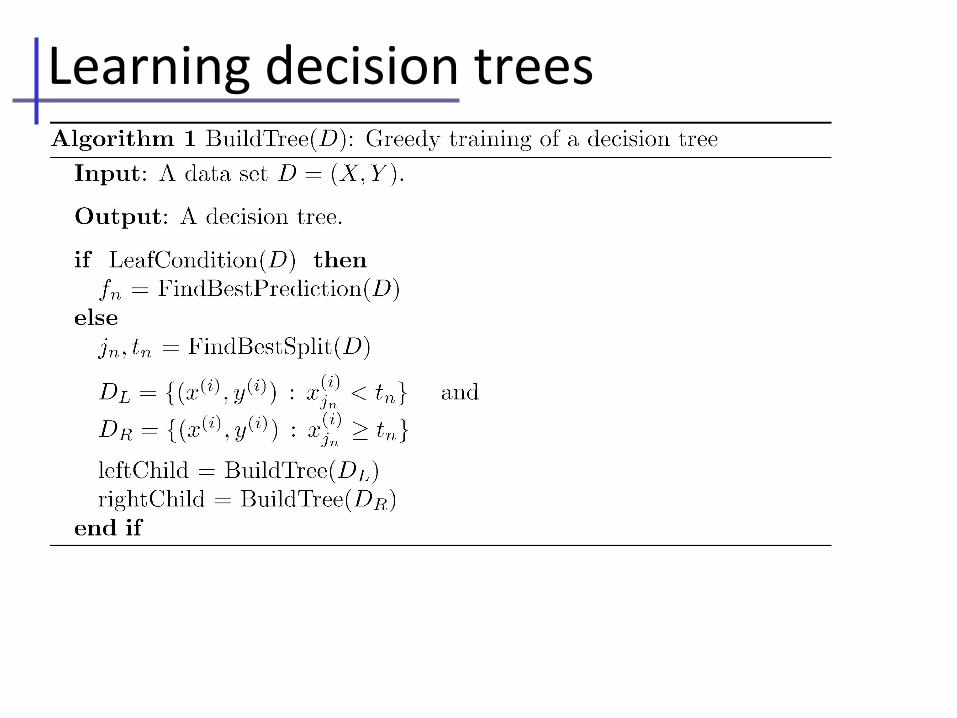
Learning decision trees• Break into two parts
– Should this be a leaf node?– If so: what should we predict?– If not: how should we further split the data?
• Leaf nodes: best prediction given this data subset– Classify: pick majority class; Regress: predict average value
• Non-leaf nodes: pick a feature and a split– Greedy: “score” all possible features and splits– Score function measures “purity” of data after split
• How much easier is our prediction task after we divide the data?
• When to make a leaf node?– All training examples the same class (correct), or indistinguishable– Fixed depth (fixed complexity decision boundary)– Others …
Example algorithms: ID3, C4.5See e.g. wikipedia, “Classification and regression tree”
Learning decision trees

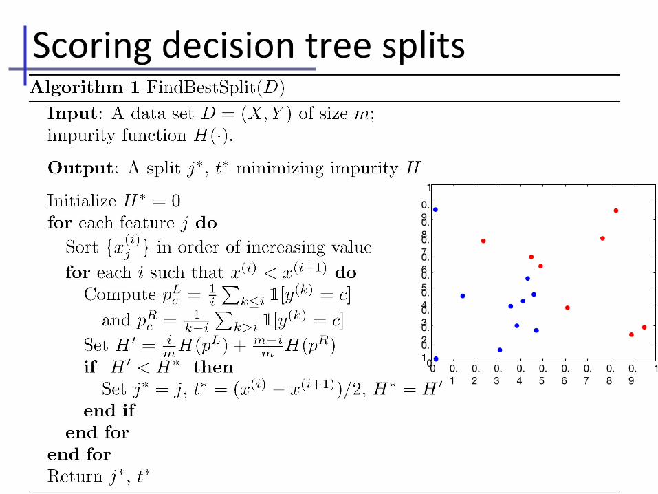
Scoring decision tree splits• How can we select which feature to split on?
– And, for real-valued features, what threshold?
[Russell & Norvig 2010]
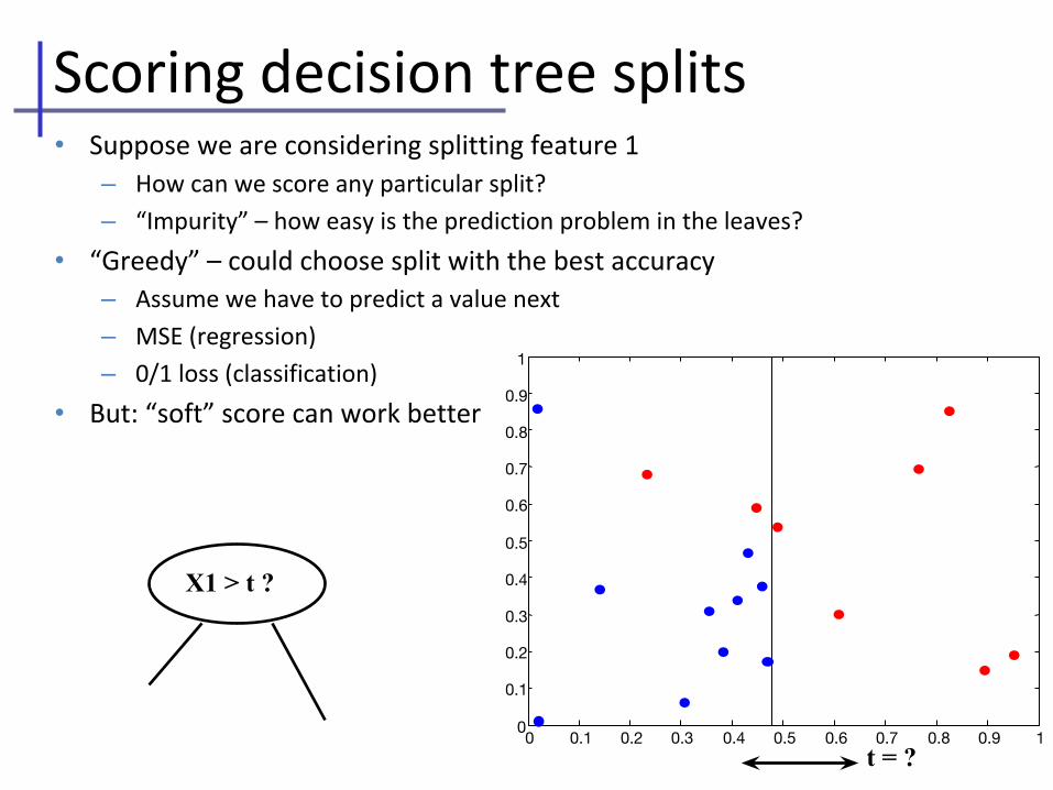
Scoring decision tree splits• Suppose we are considering splitting feature 1
– How can we score any particular split?
– “Impurity” – how easy is the prediction problem in the leaves?
• “Greedy” – could choose split with the best accuracy– Assume we have to predict a value next
– MSE (regression)
– 0/1 loss (classification)
• But: “soft” score can work better
0 0.1 0.2 0.3 0.4 0.5 0.6 0.7 0.8 0.9 10
0.1
0.2
0.3
0.4
0.5
0.6
0.7
0.8
0.9
1
X1 > t ?
t = ?
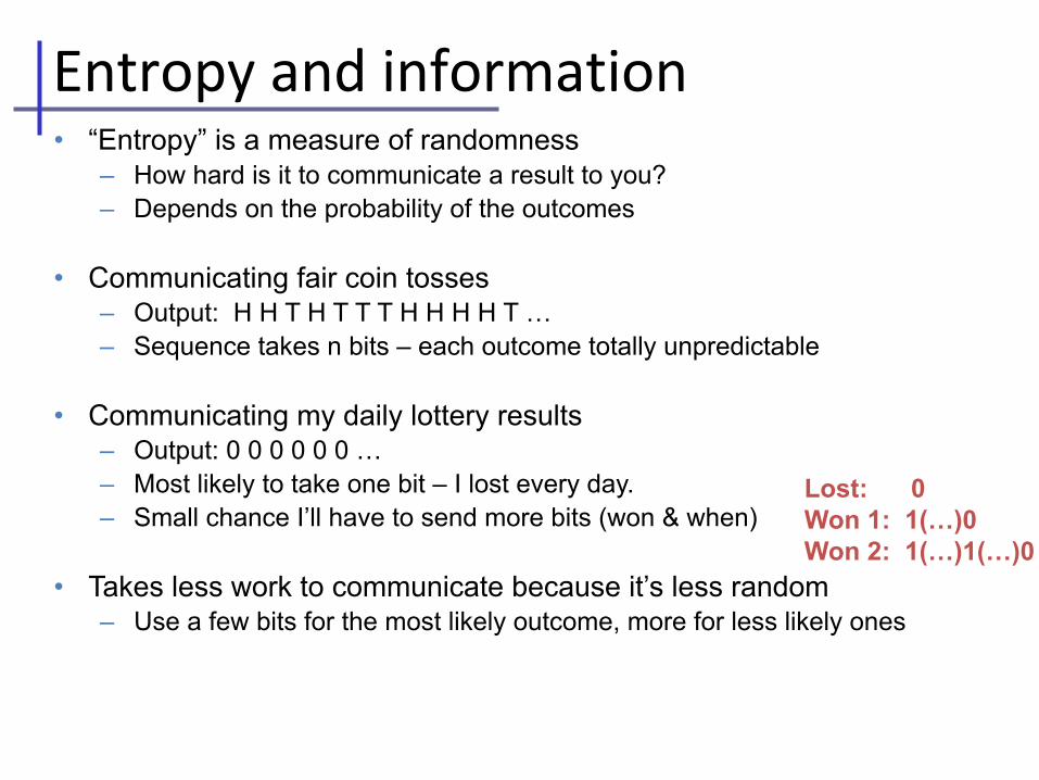
• “Entropy” is a measure of randomness– How hard is it to communicate a result to you?– Depends on the probability of the outcomes
• Communicating fair coin tosses– Output: H H T H T T T H H H H T …– Sequence takes n bits – each outcome totally unpredictable
• Communicating my daily lottery results– Output: 0 0 0 0 0 0 …– Most likely to take one bit – I lost every day.– Small chance I’ll have to send more bits (won & when)
• Takes less work to communicate because it’s less random– Use a few bits for the most likely outcome, more for less likely ones
Lost: 0Won 1: 1(…)0Won 2: 1(…)1(…)0
Entropy and information
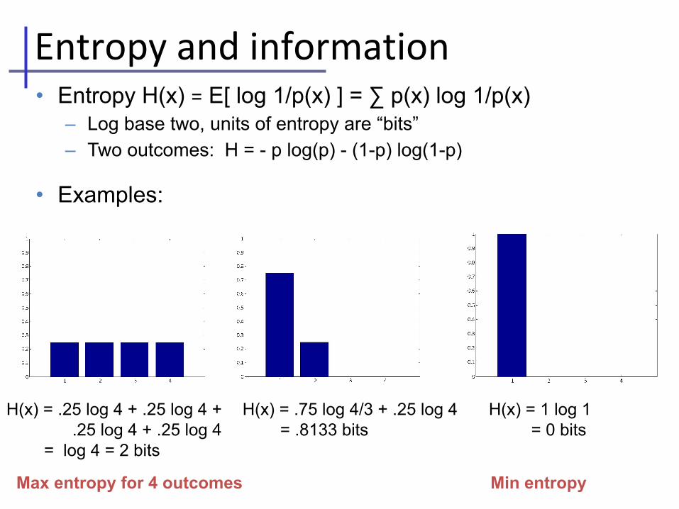
• Entropy H(x) = E[ log 1/p(x) ] = ∑ p(x) log 1/p(x)– Log base two, units of entropy are “bits”– Two outcomes: H = - p log(p) - (1-p) log(1-p)
• Examples:
H(x) = .25 log 4 + .25 log 4 + .25 log 4 + .25 log 4 = log 4 = 2 bits
H(x) = .75 log 4/3 + .25 log 4 = .8133 bits
H(x) = 1 log 1 = 0 bits
Max entropy for 4 outcomes Min entropy
Entropy and information
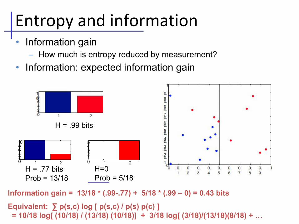
• Information gain– How much is entropy reduced by measurement?
• Information: expected information gain
1 2012345
1 20246810
H=0Prob = 5/18
H = .77 bitsProb = 13/18
H = .99 bits
Information gain = 13/18 * (.99-.77) + 5/18 * (.99 – 0) = 0.43 bits
Equivalent: ∑ p(s,c) log [ p(s,c) / p(s) p(c) ] = 10/18 log[ (10/18) / (13/18) (10/18)] + 3/18 log[ (3/18)/(13/18)(8/18) + …
Entropy and information
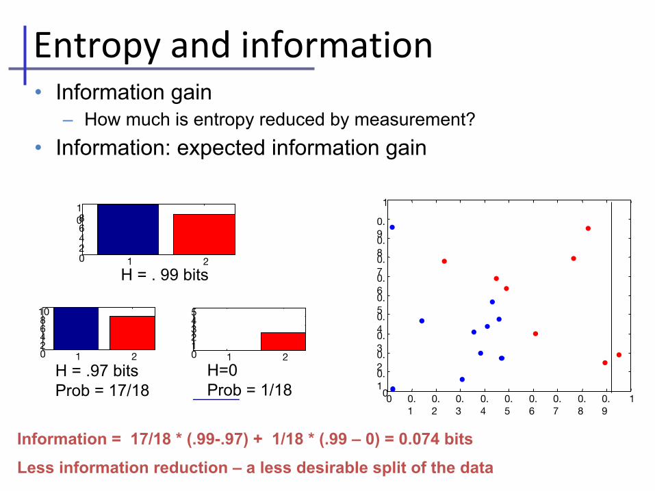
• Information gain– How much is entropy reduced by measurement?
• Information: expected information gain
0 0.1
0.2
0.3
0.4
0.5
0.6
0.7
0.8
0.9
10
0.1
0.2
0.3
0.4
0.5
0.6
0.7
0.8
0.9
1
1 20246810
1 2012345
1 20246810
H=0Prob = 1/18
H = .97 bitsProb = 17/18
H = . 99 bits
Entropy and information
Information = 17/18 * (.99-.97) + 1/18 * (.99 – 0) = 0.074 bits
Less information reduction – a less desirable split of the data
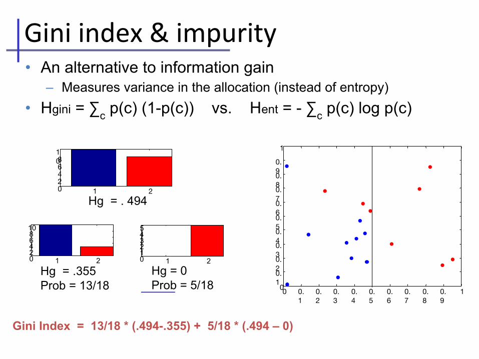
• An alternative to information gain– Measures variance in the allocation (instead of entropy)
• Hgini = ∑c p(c) (1-p(c)) vs. Hent = - ∑c p(c) log p(c)
0 0.1
0.2
0.3
0.4
0.5
0.6
0.7
0.8
0.9
10
0.1
0.2
0.3
0.4
0.5
0.6
0.7
0.8
0.9
1
1 20246810
1 2012345
1 20246810
Hg = 0Prob = 5/18
Hg = .355Prob = 13/18
Hg = . 494
Gini Index = 13/18 * (.494-.355) + 5/18 * (.494 – 0)
Gini index & impurity
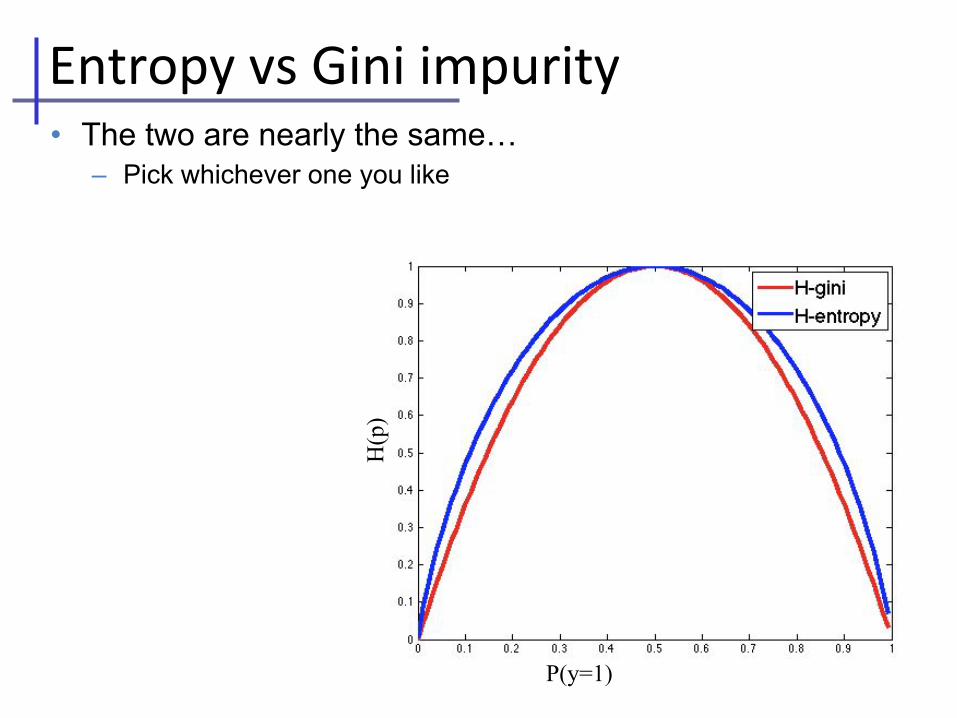
• The two are nearly the same…– Pick whichever one you like
P(y=1)
H(p
)
Entropy vs Gini impurity
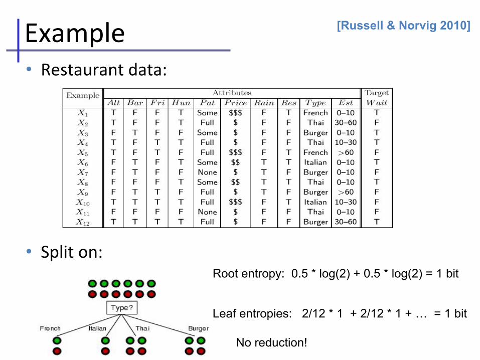
Example• Restaurant data:
• Split on:
[Russell & Norvig 2010]
Root entropy: 0.5 * log(2) + 0.5 * log(2) = 1 bit
Leaf entropies: 2/12 * 1 + 2/12 * 1 + … = 1 bit
No reduction!

Example• Restaurant data:
• Split on:Root entropy: 0.5 * log(2) + 0.5 * log(2) = 1 bit
Leaf entropies: 2/12 * 0 + 4/12 * 0 + 6/12 * 0.9
Lower entropy after split!
[Russell & Norvig 2010]

Hungry?
…
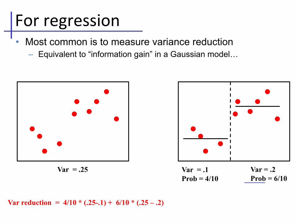
• Most common is to measure variance reduction– Equivalent to “information gain” in a Gaussian model…
Var = .2Prob = 6/10
Var = .1Prob = 4/10
Var = .25
Var reduction = 4/10 * (.25-.1) + 6/10 * (.25 – .2)
For regression
Scoring decision tree splits
0 0.1
0.2
0.3
0.4
0.5
0.6
0.7
0.8
0.9
10
0.1
0.2
0.3
0.4
0.5
0.6
0.7
0.8
0.9
1
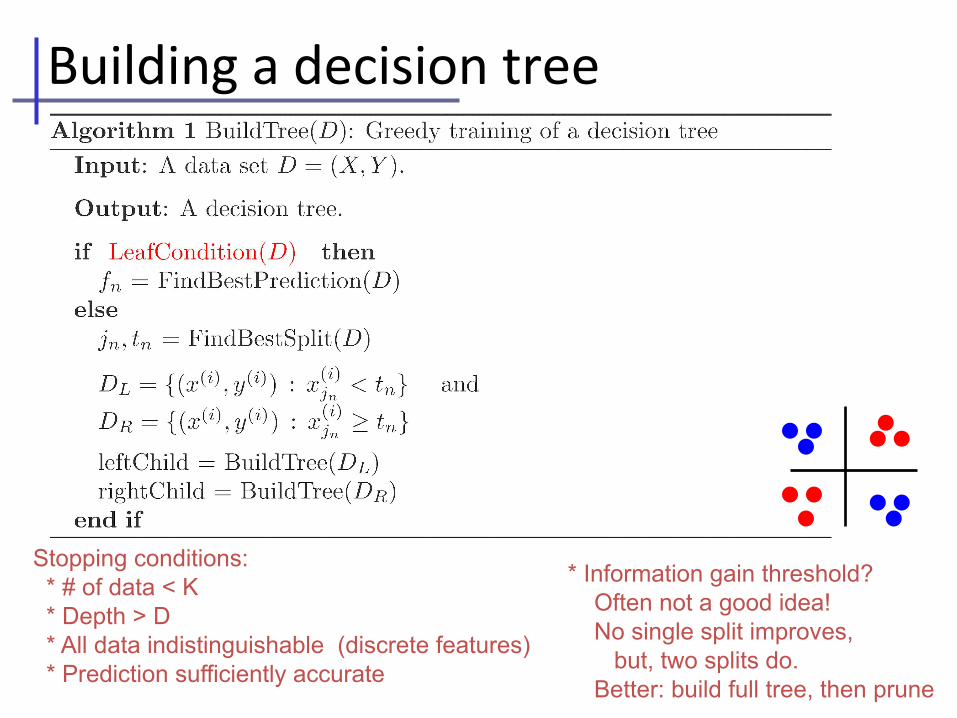
Building a decision tree
Stopping conditions: * # of data < K * Depth > D * All data indistinguishable (discrete features) * Prediction sufficiently accurate
* Information gain threshold? Often not a good idea! No single split improves, but, two splits do. Better: build full tree, then prune
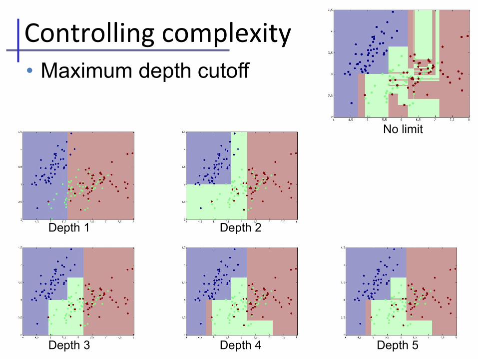
• Maximum depth cutoff
Depth 1 Depth 2
Depth 3 Depth 4 Depth 5
No limit
Controlling complexity
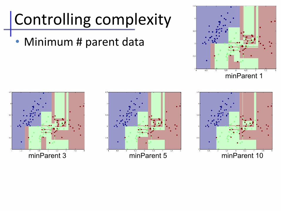
• Minimum # parent data
minParent 1
minParent 3 minParent 5 minParent 10
Controlling complexity
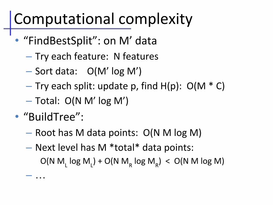
Computational complexity• “FindBestSplit”: on M’ data
– Try each feature: N features
– Sort data: O(M’ log M’)
– Try each split: update p, find H(p): O(M * C)
– Total: O(N M’ log M’)
• “BuildTree”:– Root has M data points: O(N M log M)
– Next level has M *total* data points: O(N M
L log M
L) + O(N M
R log M
R) < O(N M log M)
– …
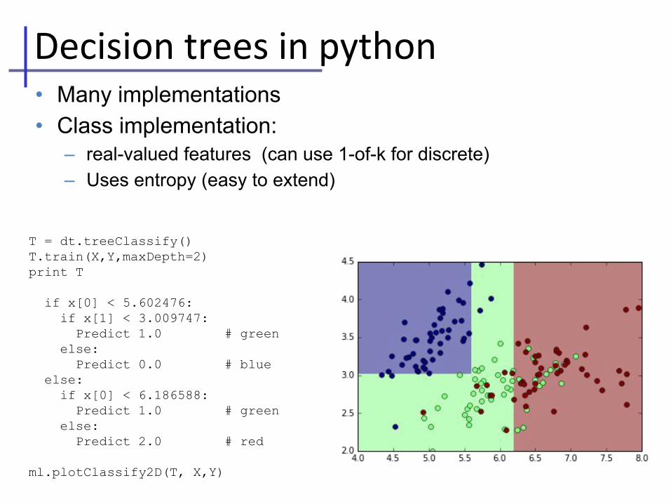
• Many implementations• Class implementation:
– real-valued features (can use 1-of-k for discrete)– Uses entropy (easy to extend)
T = dt.treeClassify()T.train(X,Y,maxDepth=2)print T
if x[0] < 5.602476: if x[1] < 3.009747: Predict 1.0 # green else: Predict 0.0 # blue else: if x[0] < 6.186588: Predict 1.0 # green else: Predict 2.0 # red ml.plotClassify2D(T, X,Y)
Decision trees in python
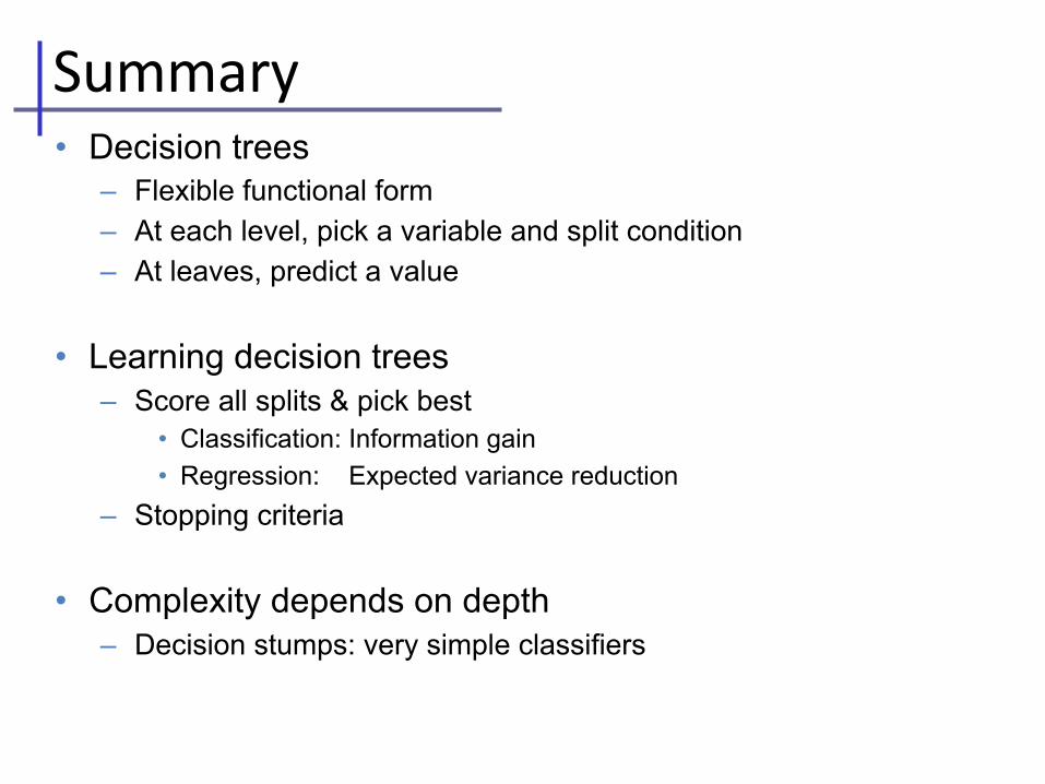
• Decision trees– Flexible functional form– At each level, pick a variable and split condition– At leaves, predict a value
• Learning decision trees– Score all splits & pick best
• Classification: Information gain• Regression: Expected variance reduction
– Stopping criteria
• Complexity depends on depth– Decision stumps: very simple classifiers
Summary


![Graph Edge Coloring: Tashkinov Trees and Goldberg’s … · Graph Edge Coloring: Tashkinov Trees and Goldberg’s Conjecture ... [13, 14] a simple but very ... tional edge coloring](https://static.fdocument.org/doc/165x107/5af8fa657f8b9aac248dd47f/graph-edge-coloring-tashkinov-trees-and-goldbergs-edge-coloring-tashkinov.jpg)


![Maroussi, 4-6-2013 Decision no. 693/9 DECISION Regulation ...Maroussi, 4-6-2013 Decision no. 693/9 DECISION «Regulation on Management and Assignment of [.gr] Domain Names» The Hellenic](https://static.fdocument.org/doc/165x107/5ff09edd49cda41bcc425ac3/maroussi-4-6-2013-decision-no-6939-decision-regulation-maroussi-4-6-2013.jpg)