Decimation filters for Σ∆ ADCs - University of California, …€“ A 30kHz LPF provides only...
40
EECS 247 Lecture 19: Decimation Filters © 2002 B. Boser 1 A/D DSP Decimation filters for Σ∆ ADCs • Digital decimation filters – Aliasing in the analog domain – Aliasing in the digital domain – Coefficient precision and gain scaling • Digital arithmetic throughput calculations – One-stage decimation – Linear phase implications – Multi-stage decimation Ref: R. E. Crochiere and L. R. Rabiner, “Interpolation and Decimation of Digital Signals – A Tutorial Review”, Proc. IEEE, 69 , pp. 300-331, March 1981. EECS 247 Lecture 19: Decimation Filters © 2002 B. Boser 2 A/D DSP Σ∆ Analog-to-Digital Converters •A Σ∆ Analog-to-Digital Converter (Σ∆ ADC) combines – An analog Σ∆ modulator which produces an oversampled output stream of 1-bit digital samples – A digital decimation filter which takes the 1-bit modulator output as its input and • Filters out out-of-band quantization noise • Filters out unwanted out-of-band signals present in the modulator’s analog input • Lowers the sampling frequency to a value closer to 2X the highest frequency of interest
Transcript of Decimation filters for Σ∆ ADCs - University of California, …€“ A 30kHz LPF provides only...
EECS 247 Lecture 19: Decimation Filters © 2002 B. Boser 1A/DDSP
Decimation filters for Σ∆ ADCs• Digital decimation filters
– Aliasing in the analog domain– Aliasing in the digital domain– Coefficient precision and gain scaling
• Digital arithmetic throughput calculations– One-stage decimation– Linear phase implications– Multi-stage decimation
Ref: R. E. Crochiere and L. R. Rabiner, “Interpolation and Decimation of Digital Signals – A Tutorial Review”, Proc. IEEE, 69, pp. 300-331, March 1981.
EECS 247 Lecture 19: Decimation Filters © 2002 B. Boser 2A/DDSP
Σ∆ Analog-to-Digital Converters• A Σ∆ Analog-to-Digital Converter (Σ∆ ADC)
combines– An analog Σ∆ modulator which produces an
oversampled output stream of 1-bit digital samples– A digital decimation filter which takes the 1-bit
modulator output as its input and• Filters out out-of-band quantization noise• Filters out unwanted out-of-band signals present in the
modulator’s analog input• Lowers the sampling frequency to a value closer to 2X
the highest frequency of interest
EECS 247 Lecture 19: Decimation Filters © 2002 B. Boser 3A/DDSP
Σ∆ ADCs• Commercial DSPs aren’t designed to handle 1-bit
input samples at oversampled data rates– A 400Mip DSP only executes 133 instructions per 3MHz
sample– In 2001, the 32X32b multiply-accumulate cost is 5¢/Mip*,
independent of the number of active bits/word• DSPs are designed to handle 16+ bit wide data
words at Nyquist-like sampling frequencies• Σ∆ decimation filters bridge the speed/resolution gap
*Ref: Texas Instruments, C2000 Series DSP datasheets, 2001.
EECS 247 Lecture 19: Decimation Filters © 2002 B. Boser 4A/DDSP
Aliasing in the Analog Domain• We’ll continue using the 3MHz, 1-bit Σ∆ modulator
and its audio application as the basis for decimation filter analysis
• Sampling action at the modulator input inherently results in aliasing– 2980 and 3020kHz alias to 20kHz– 2999 and 3001kHz alias to 1kHz
• No digital filter can separate frequency components that have aliased on top of one another
EECS 247 Lecture 19: Decimation Filters © 2002 B. Boser 5A/DDSP
Aliasing in the Analog Domain• 1st-order RC filters usually provide adequate
antialiasing protection for Σ∆ ADCs– A 30kHz LPF provides only 40dB of attenuation at 3MHz,– But microphones and other audio transducers produce
negligible outputs at 3MHz
• “Transducer loss” is an important factor in all real-world antialiasing filter specifications– Talk to veterans about the level of transducer loss you can
count on in your application– Or measure it
EECS 247 Lecture 19: Decimation Filters © 2002 B. Boser 6A/DDSP
Aliasing in the Analog Domain• Protecting high-order modulators from instability-
provoking square wave inputs provides additional justification for an RC antialiasing filter
• Remember that any RC antialiasing filter adds kT/C noise– Almost all of this noise is in the band of interest– Let’s review a 600Ω, 10nF LPF …
EECS 247 Lecture 19: Decimation Filters © 2002 B. Boser 7A/DDSP
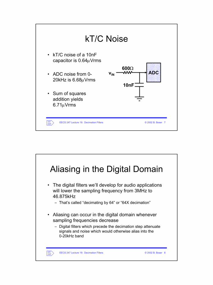
kT/C Noise• kT/C noise of a 10nF
capacitor is 0.64µVrms
• ADC noise from 0-20kHz is 6.68µVrms
• Sum of squares addition yields 6.71µVrms
600Ω
10nF
vIN ADC
EECS 247 Lecture 19: Decimation Filters © 2002 B. Boser 8A/DDSP
Aliasing in the Digital Domain• The digital filters we’ll develop for audio applications
will lower the sampling frequency from 3MHz to 46.875kHz– That’s called “decimating by 64” or “64X decimation”
• Aliasing can occur in the digital domain whenever sampling frequencies decrease– Digital filters which precede the decimation step attenuate
signals and noise which would otherwise alias into the 0-20kHz band
EECS 247 Lecture 19: Decimation Filters © 2002 B. Boser 9A/DDSP
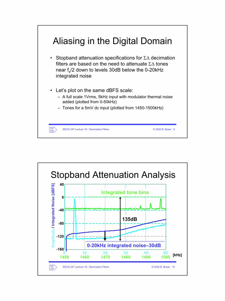
Aliasing in the Digital Domain• Stopband attenuation specifications for Σ∆ decimation
filters are based on the need to attenuate Σ∆ tones near fs/2 down to levels 30dB below the 0-20kHz integrated noise
• Let’s plot on the same dBFS scale:– A full scale 1Vrms, 5kHz input with modulator thermal noise
added (plotted from 0-50kHz)– Tones for a 5mV dc input (plotted from 1450-1500kHz)
EECS 247 Lecture 19: Decimation Filters © 2002 B. Boser 10A/DDSP
Stopband Attenuation Analysis
[kHz]
0
-40
-120
-160
40
-80
0 40302010 50
integrated tone bins
0-20kHz integrated noise–30dBAm
plitu
de /
Inte
grat
ed N
oise
[dB
FS]
1450 1490148014701460 1500
135dB
EECS 247 Lecture 19: Decimation Filters © 2002 B. Boser 11A/DDSP
Stopband Attenuation Analysis• 135dB of stopband attenuation is required for aliased
tone suppression– Digital filter coefficient precision rule-of-thumb: 6dB/bit– 135 / 6 = 22.5 … round to 24b FIR filter coefficients
• 135dB of stopband attenuation results in negligible aliased non-tonal quantization noise
• Where should the stopband begin?– Given our decimation filter output word rate of 46.875kHz,
23kHz seems a safe choice
EECS 247 Lecture 19: Decimation Filters © 2002 B. Boser 12A/DDSP
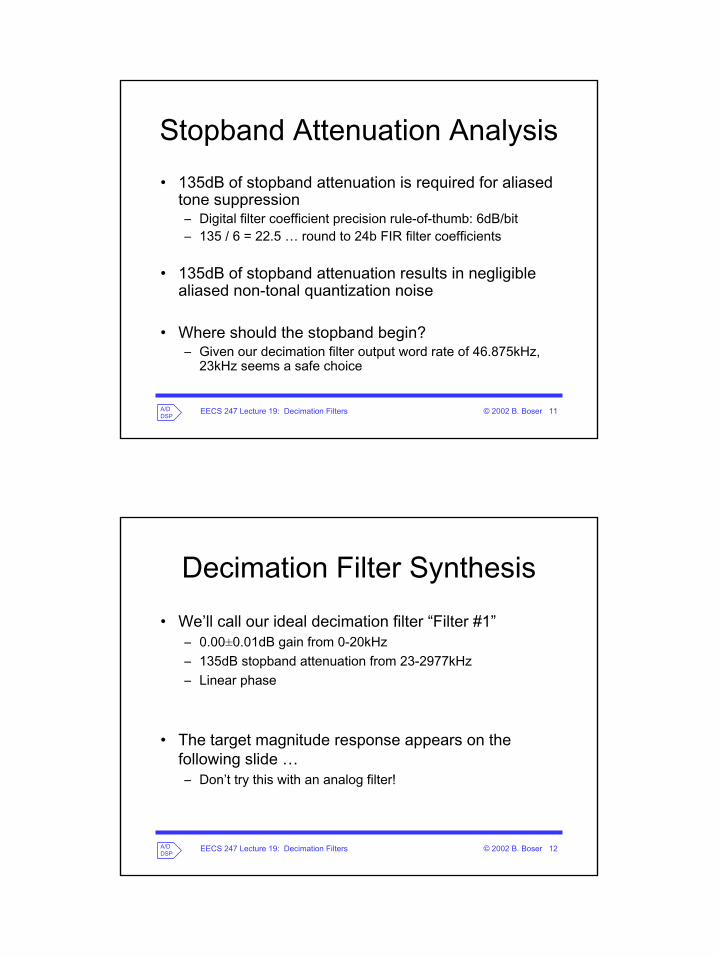
Decimation Filter Synthesis• We’ll call our ideal decimation filter “Filter #1”
– 0.00±0.01dB gain from 0-20kHz– 135dB stopband attenuation from 23-2977kHz– Linear phase
• The target magnitude response appears on the following slide …– Don’t try this with an analog filter!
EECS 247 Lecture 19: Decimation Filters © 2002 B. Boser 13A/DDSP
Filter #1 Target Response
[kHz]
Dec
imat
ion
Filte
r Gai
n (d
B)
0
-40
-120
-160
40
-80
0 40302010 50
5mV dc inputnoise shape
EECS 247 Lecture 19: Decimation Filters © 2002 B. Boser 14A/DDSP
Decimation Filter Synthesis
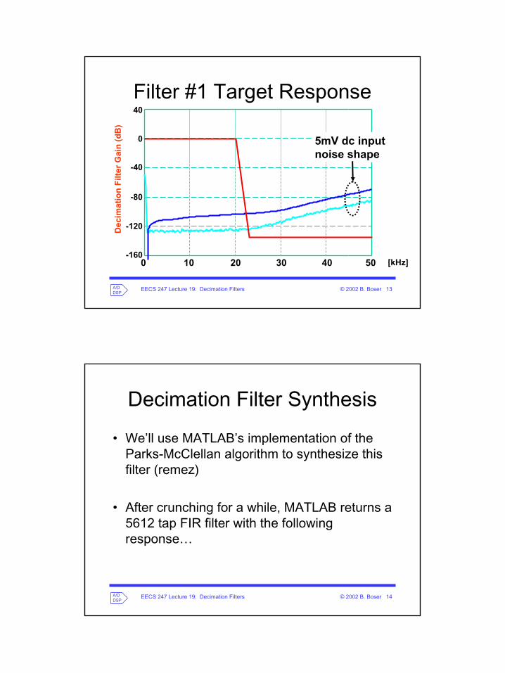
• We’ll use MATLAB’s implementation of the Parks-McClellan algorithm to synthesize this filter (remez)
• After crunching for a while, MATLAB returns a 5612 tap FIR filter with the following response…
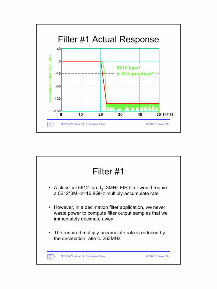
EECS 247 Lecture 19: Decimation Filters © 2002 B. Boser 15A/DDSP
Filter #1 Actual ResponseD
ecim
atio
n Fi
lter G
ain
(dB
)
0
-40
-120
-160
40
-80
0 40302010 50
5612 taps!Is this practical?
[kHz]
EECS 247 Lecture 19: Decimation Filters © 2002 B. Boser 16A/DDSP
Filter #1• A classical 5612-tap, fS=3MHz FIR filter would require
a 5612*3MHz=16.8GHz multiply-accumulate rate
• However, in a decimation filter application, we never waste power to compute filter output samples that we immediately decimate away
• The required multiply-accumulate rate is reduced by the decimation ratio to 263MHz
EECS 247 Lecture 19: Decimation Filters © 2002 B. Boser 17A/DDSP
Filter #1
• The second key factor that makes this FIR filter unusual is that it needs no hardware multiplier at all– Input data is only 1-bit wide– The “multiplier” merely adds or subtracts coefficients from
the accumulator
• 263MHz begins to seem reasonable, but we can use another simple trick to reduce power further …
EECS 247 Lecture 19: Decimation Filters © 2002 B. Boser 18A/DDSP
Coefficient Symmetry• Linear phase filter coefficients are symmetric around
the middle of the impulse response
• We’d never waste ROM to store all 5612 coefficients when only 2806 are unique
• A 5612x1b data memory allows us to exploit coefficient symmetry to reduce “multiply”-accumulate rates by another 2X …
EECS 247 Lecture 19: Decimation Filters © 2002 B. Boser 19A/DDSP
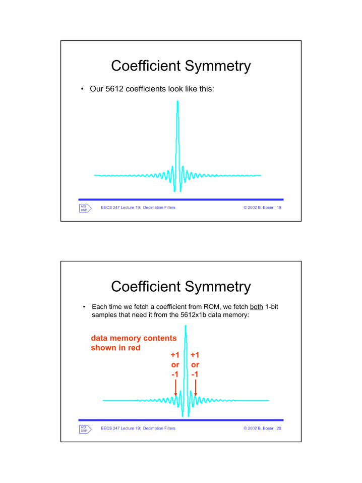
Coefficient Symmetry• Our 5612 coefficients look like this:
EECS 247 Lecture 19: Decimation Filters © 2002 B. Boser 20A/DDSP
Coefficient Symmetry• Each time we fetch a coefficient from ROM, we fetch both 1-bit
samples that need it from the 5612x1b data memory:
+1or-1
+1or-1
data memory contentsshown in red
EECS 247 Lecture 19: Decimation Filters © 2002 B. Boser 21A/DDSP
Coefficient Symmetry• We only have two data states, +1 and –1
• If we add the data before “multiplying”, only 3 results are possible:– +2 if both 1b samples are +1– -2 if both 1b samples are –1– 0 if 1b samples are –1,+1 or +1,-1– Our “multiplier-accumulator” adds, subtracts, or does nothing
• “Multiply-accumulate” in this application requires only an accumulator operating at 132MHz!
EECS 247 Lecture 19: Decimation Filters © 2002 B. Boser 22A/DDSP
Filter #2• While the throughput requirements of Filter #1 are not
outrageous, audio applications economize further
• Modulator input signals that alias into frequencies above 20kHz are inaudible– Most people can’t hear 20kHz full-scale sinewaves– Who would ever record that anyway?
• So, unless you’re interested in marketing your audio ADC to dogs (dogs can hear up to 30kHz, supposedly), consider Filter #2 …
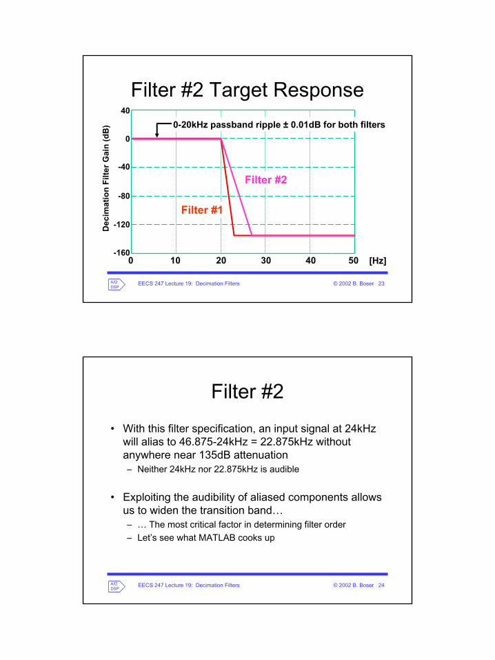
EECS 247 Lecture 19: Decimation Filters © 2002 B. Boser 23A/DDSP
Filter #2 Target Response
[Hz]
Dec
imat
ion
Filte
r Gai
n (d
B)
0
-40
-120
-160
40
-80
0 40302010 50
Filter #1
Filter #2
0-20kHz passband ripple ± 0.01dB for both filters
EECS 247 Lecture 19: Decimation Filters © 2002 B. Boser 24A/DDSP
Filter #2• With this filter specification, an input signal at 24kHz
will alias to 46.875-24kHz = 22.875kHz without anywhere near 135dB attenuation– Neither 24kHz nor 22.875kHz is audible
• Exploiting the audibility of aliased components allows us to widen the transition band…– … The most critical factor in determining filter order– Let’s see what MATLAB cooks up
EECS 247 Lecture 19: Decimation Filters © 2002 B. Boser 25A/DDSP
Filter #2 Actual Response
[kHz]
Dec
imat
ion
Filte
r Gai
n (d
B)
0
-40
-120
-160
40
-80
0 40302010 50
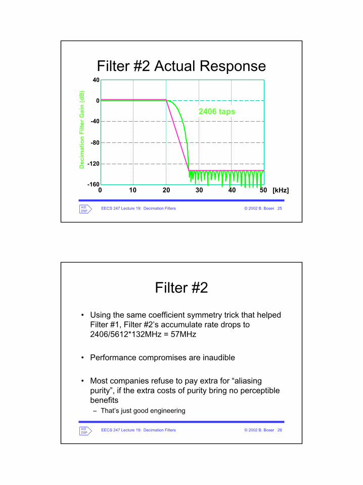
2406 taps
EECS 247 Lecture 19: Decimation Filters © 2002 B. Boser 26A/DDSP
Filter #2• Using the same coefficient symmetry trick that helped
Filter #1, Filter #2’s accumulate rate drops to 2406/5612*132MHz = 57MHz
• Performance compromises are inaudible
• Most companies refuse to pay extra for “aliasing purity”, if the extra costs of purity bring no perceptible benefits– That’s just good engineering
EECS 247 Lecture 19: Decimation Filters © 2002 B. Boser 27A/DDSP
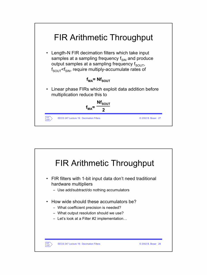
FIR Arithmetic Throughput• Length-N FIR decimation filters which take input
samples at a sampling frequency fSIN and produce output samples at a sampling frequency fSOUT, fSOUT<fSIN, require multiply-accumulate rates of
• Linear phase FIRs which exploit data addition before multiplication reduce this to
fMA= NfSOUT
fMA= NfSOUT
2
EECS 247 Lecture 19: Decimation Filters © 2002 B. Boser 28A/DDSP
FIR Arithmetic Throughput• FIR filters with 1-bit input data don’t need traditional
hardware multipliers– Use add/subtract/do nothing accumulators
• How wide should these accumulators be?– What coefficient precision is needed?– What output resolution should we use?– Let’s look at a Filter #2 implementation…
EECS 247 Lecture 19: Decimation Filters © 2002 B. Boser 29A/DDSP
FIR Implementation• Digital filters usually come with bit-width’ that are
multiples of 4• 16-bits results in unwanted digital quantization noise• So let’s try a 20-bit filter for our 16-bit ADC
– 220=1048576– Each LSB is 1ppm of the ADC input range
• Let’s look at the mapping of our 1Vrms full scale sinewave into digital output values– Before we set filter gain levels, we need to review modulator
outputs
EECS 247 Lecture 19: Decimation Filters © 2002 B. Boser 30A/DDSP
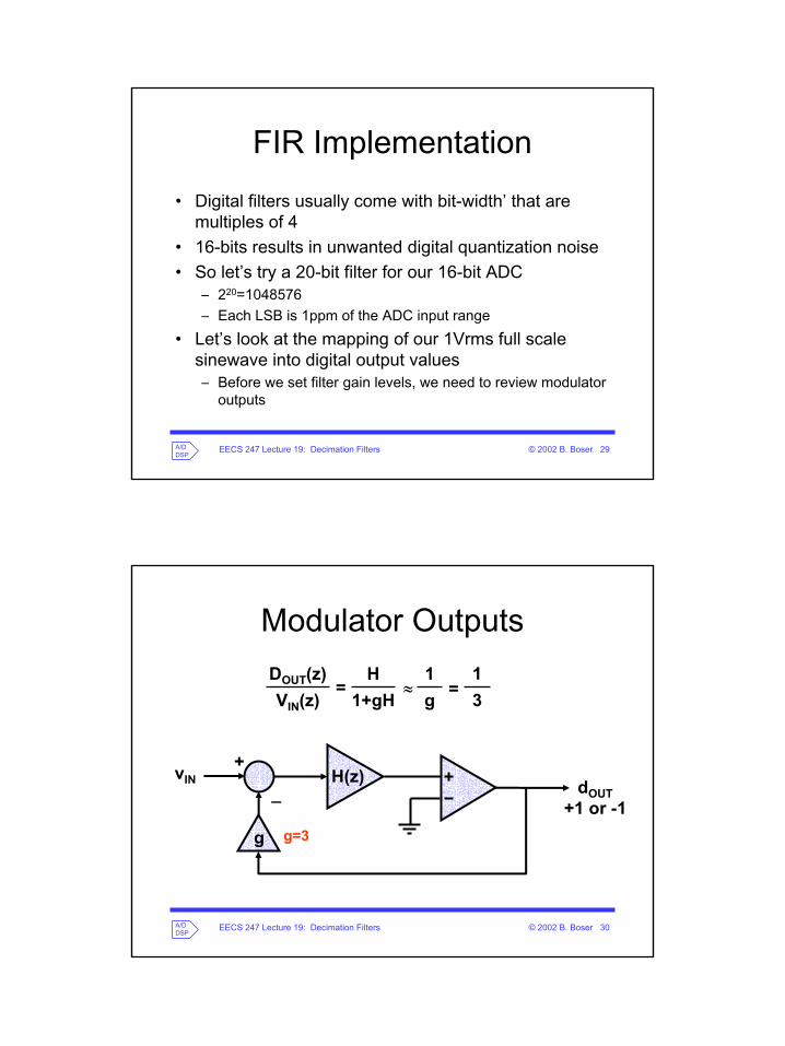
Modulator Outputs
H(z)+
_vIN dOUT
+1 or -1g
DOUT(z)VIN(z)
≈1g
g=3
=H
1+gH13=
EECS 247 Lecture 19: Decimation Filters © 2002 B. Boser 31A/DDSP
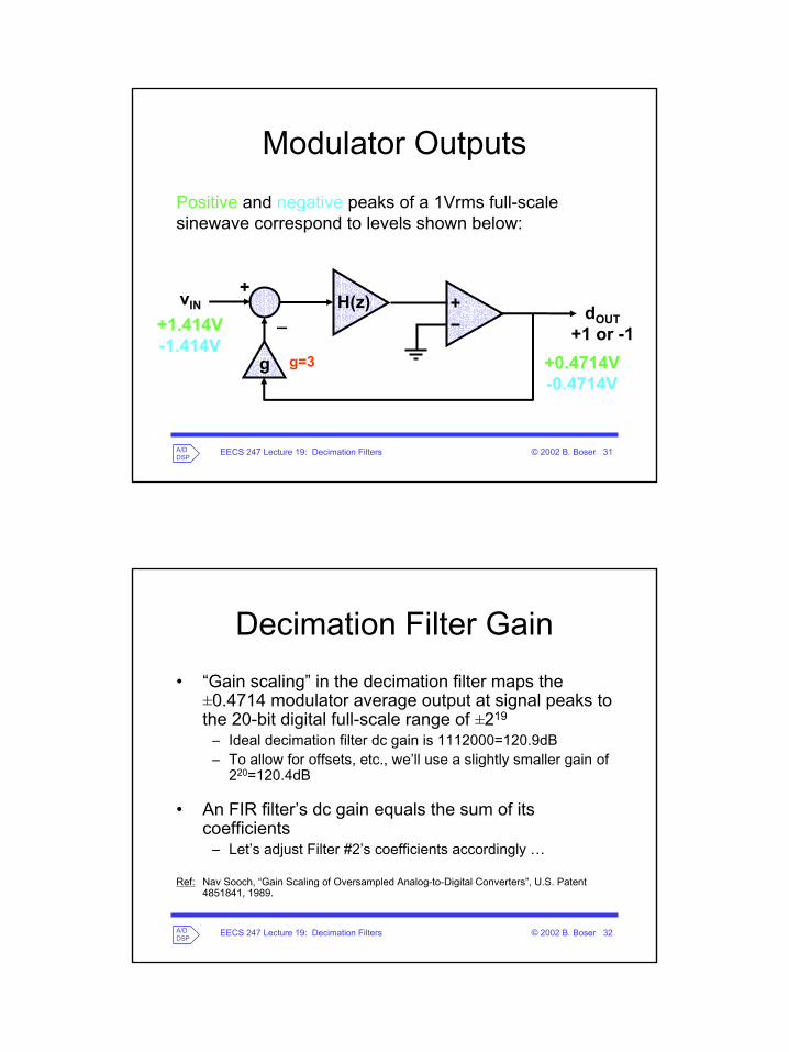
Modulator OutputsPositive and negative peaks of a 1Vrms full-scale sinewave correspond to levels shown below:
H(z)+
_vIN dOUT
+1 or -1g g=3
+1.414V-1.414V
+0.4714V-0.4714V
EECS 247 Lecture 19: Decimation Filters © 2002 B. Boser 32A/DDSP
Decimation Filter Gain• “Gain scaling” in the decimation filter maps the ±0.4714 modulator average output at signal peaks to the 20-bit digital full-scale range of ±219
– Ideal decimation filter dc gain is 1112000=120.9dB– To allow for offsets, etc., we’ll use a slightly smaller gain of
220=120.4dB
• An FIR filter’s dc gain equals the sum of its coefficients
– Let’s adjust Filter #2’s coefficients accordingly …
Ref: Nav Sooch, “Gain Scaling of Oversampled Analog-to-Digital Converters”, U.S. Patent 4851841, 1989.
EECS 247 Lecture 19: Decimation Filters © 2002 B. Boser 33A/DDSP
Filter #2 Response
[kHz]
Dec
imat
ion
Filte
r Gai
n (d
B)
120
80
0
-40
160
40
0 40302010 50
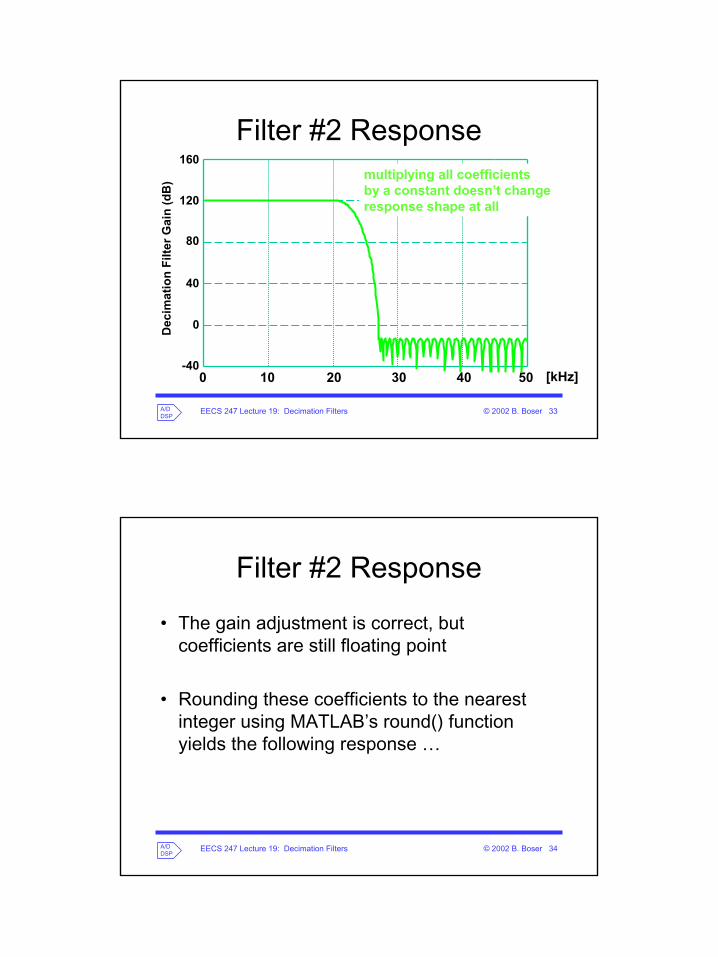
multiplying all coefficientsby a constant doesn’t changeresponse shape at all
EECS 247 Lecture 19: Decimation Filters © 2002 B. Boser 34A/DDSP
Filter #2 Response
• The gain adjustment is correct, but coefficients are still floating point
• Rounding these coefficients to the nearest integer using MATLAB’s round() function yields the following response …
EECS 247 Lecture 19: Decimation Filters © 2002 B. Boser 35A/DDSP
Filter #2 Responses
[kHz]
Dec
imat
ion
Filte
r Gai
n (d
B)
120
80
0
-40
160
40
0 40302010 50
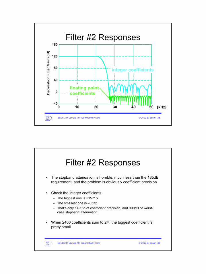
integer coefficients
floating point coefficients
EECS 247 Lecture 19: Decimation Filters © 2002 B. Boser 36A/DDSP
Filter #2 Responses• The stopband attenuation is horrible, much less than the 135dB
requirement, and the problem is obviously coefficient precision
• Check the integer coefficients– The biggest one is +15715– The smallest one is –3332– That’s only 14-15b of coefficient precision, and <90dB of worst-
case stopband attenuation
• When 2406 coefficients sum to 220, the biggest coefficient is pretty small
EECS 247 Lecture 19: Decimation Filters © 2002 B. Boser 37A/DDSP
Filter #2 Bit MapLet’s look at the digital scaling in our defective filter :
15 14 13 12 11 10 9 8 7 6 5 4 3 2 1 016171819
0
14 13 12 11 10 9 8 7 6 5 4 3 2 1 0
1b data
rounded coef.
accumulator
15 14 13 12 11 10 9 8 7 6 5 4 3 2 1 016171819 ADC output
EECS 247 Lecture 19: Decimation Filters © 2002 B. Boser 38A/DDSP
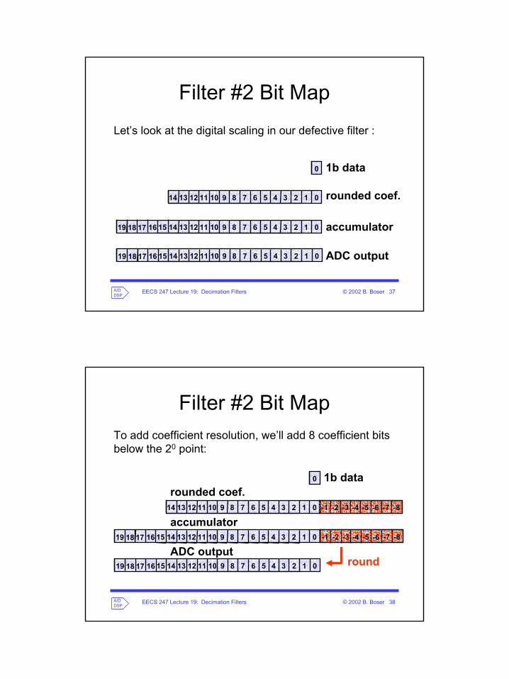
Filter #2 Bit MapTo add coefficient resolution, we’ll add 8 coefficient bits below the 20 point:
15 14 13 12 11 10 9 8 7 6 5 4 3 2 1 016171819
0
14 13 12 11 10 9 8 7 6 5 4 3 2 1 0
1b datarounded coef.
accumulator
15 14 13 12 11 10 9 8 7 6 5 4 3 2 1 016171819
ADC output
-1 -2 -3 -4 -5 -7 -8-6
-1 -2 -3 -4 -5 -7 -8-6
round
EECS 247 Lecture 19: Decimation Filters © 2002 B. Boser 39A/DDSP
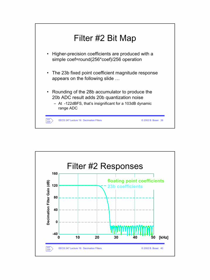
Filter #2 Bit Map• Higher-precision coefficients are produced with a
simple coef=round(256*coef)/256 operation
• The 23b fixed point coefficient magnitude response appears on the following slide …
• Rounding of the 28b accumulator to produce the 20b ADC result adds 20b quantization noise– At -122dBFS, that’s insignificant for a 103dB dynamic
range ADC
EECS 247 Lecture 19: Decimation Filters © 2002 B. Boser 40A/DDSP
Filter #2 Responses
[kHz]
Dec
imat
ion
Filte
r Gai
n (d
B)
120
80
0
-40
160
40
0 40302010 50
floating point coefficients23b coefficients
EECS 247 Lecture 19: Decimation Filters © 2002 B. Boser 41A/DDSP
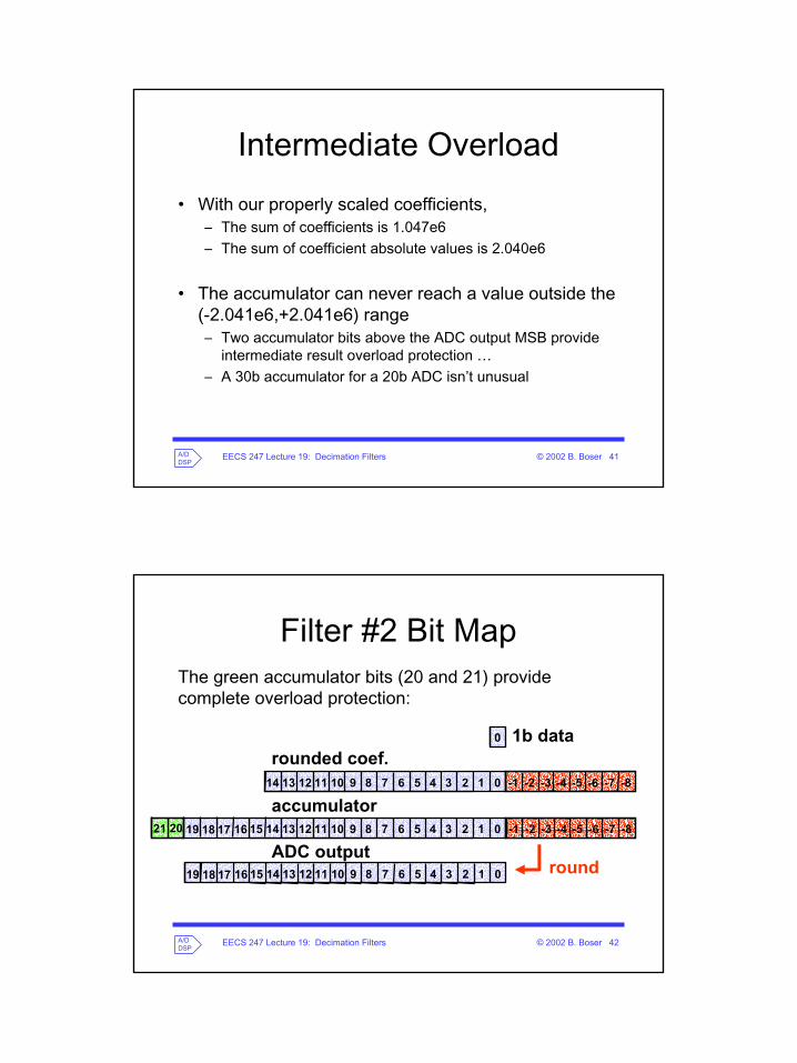
Intermediate Overload• With our properly scaled coefficients,
– The sum of coefficients is 1.047e6– The sum of coefficient absolute values is 2.040e6
• The accumulator can never reach a value outside the (-2.041e6,+2.041e6) range– Two accumulator bits above the ADC output MSB provide
intermediate result overload protection …– A 30b accumulator for a 20b ADC isn’t unusual
EECS 247 Lecture 19: Decimation Filters © 2002 B. Boser 42A/DDSP
Filter #2 Bit MapThe green accumulator bits (20 and 21) provide complete overload protection:
15 14 13 12 11 10 9 8 7 6 5 4 3 2 1 016171819
0
14 13 12 11 10 9 8 7 6 5 4 3 2 1 0
1b datarounded coef.
accumulator
15 14 13 12 11 10 9 8 7 6 5 4 3 2 1 016171819
ADC output
-1 -2 -3 -4 -5 -7 -8-6
-1 -2 -3 -4 -5 -7 -8-6
round
21 20
EECS 247 Lecture 19: Decimation Filters © 2002 B. Boser 43A/DDSP
Intermediate Overload
• Given the relatively low cost of this overload protection, it hardly pays to evaluate whether or not accumulator bit 21 can be reached by real-world ADC input signals
• Our first pass decimation filter design is complete– We’ll add this filter to our stage 2 modulator model next time
EECS 247 Lecture 19: Decimation Filters © 2002 B. Boser 44A/DDSP
Σ∆ ADC Output DFT
[kHz]
Am
plitu
de o
rInt
egra
ted
Noi
se [d
BFS
] 0
-40
-120
-160
-80
0 2015105 25
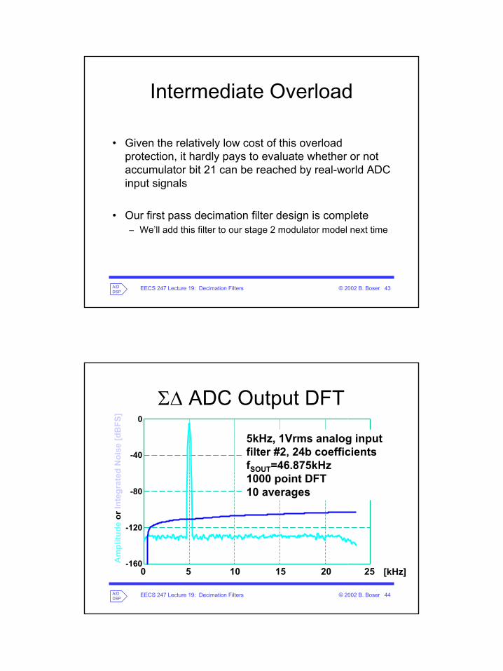
5kHz, 1Vrms analog inputfilter #2, 24b coefficients fSOUT=46.875kHz1000 point DFT10 averages
EECS 247 Lecture 19: Decimation Filters © 2002 B. Boser 45A/DDSP
Σ∆ ADC Output DFTA
mpl
itude
orIn
tegr
ated
Noi
se [d
BFS
] 0
-40
-120
-160
-80
0 2015105 25 [kHz]
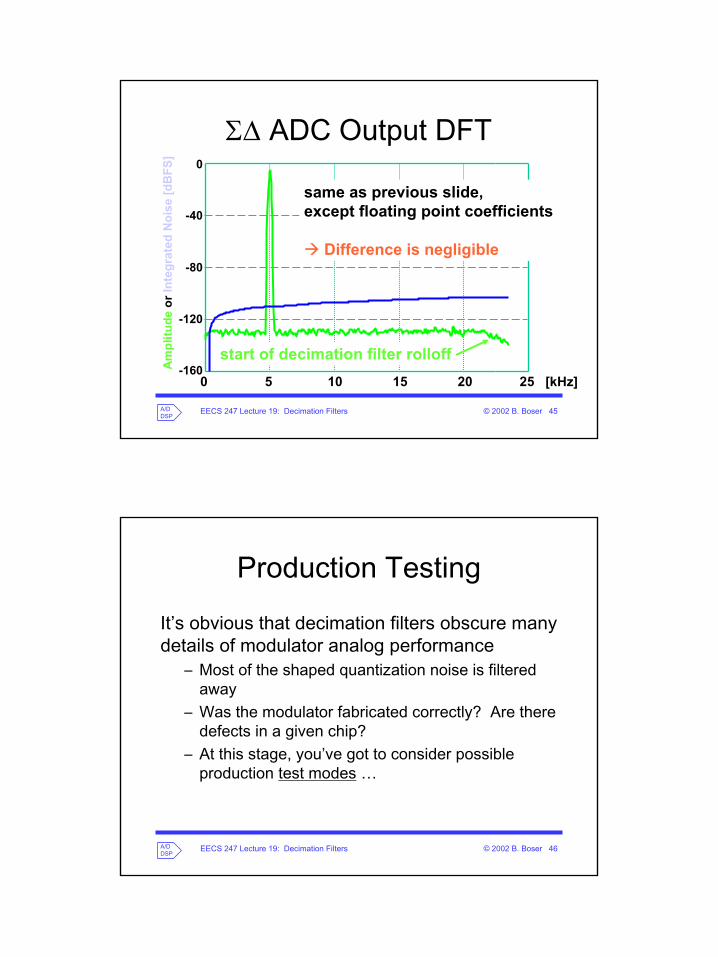
same as previous slide, except floating point coefficients
Difference is negligible
start of decimation filter rolloff
EECS 247 Lecture 19: Decimation Filters © 2002 B. Boser 46A/DDSP
Production Testing
It’s obvious that decimation filters obscure many details of modulator analog performance
– Most of the shaped quantization noise is filtered away
– Was the modulator fabricated correctly? Are there defects in a given chip?
– At this stage, you’ve got to consider possible production test modes …
EECS 247 Lecture 19: Decimation Filters © 2002 B. Boser 47A/DDSP
Test Modes• All Σ∆ ADC designs must provide at least the
following test modes:– Output unfiltered 1-bit modulator output samples– Insert test vectors at the decimation filter input
• Any mixed-signal IC which includes an ADC must provide for observability of unprocessed ADC output samples– Think of it as fault coverage in the analog domain
• Let’s see how our decimation filter obscures a typical modulator manufacturing defect …
EECS 247 Lecture 19: Decimation Filters © 2002 B. Boser 48A/DDSP
Test Modes• Suppose the modulator is built with an open fault in a
metal trace which connects up the switched capacitor implementing the b2 capacitor– b2 sets one of the quantization noise zeroes– If the b2 capacitor is missing, b2=0– In the real world, this defect will occur in 1-10ppm of
production units
• The next two slides highlight the loop filter defect, and show decimated DFTs with and without the defect
EECS 247 Lecture 19: Decimation Filters © 2002 B. Boser 49A/DDSP
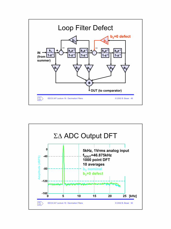
Loop Filter Defect
_k1
1-z-1++
_
+
b1
a2
b2
a1 a3 a4 a5
IN(fromsummer)
OUT (to comparator)
k2z-1
1-z-1
k3z-1
1-z-1
k4z-1
1-z-1
k5z-1
1-z-1
b2=0 defect
EECS 247 Lecture 19: Decimation Filters © 2002 B. Boser 50A/DDSP
Σ∆ ADC Output DFT
Am
plitu
de (d
BFS
)
0
-40
-120
-160
-80
0 2015105 25 [kHz]
5kHz, 1Vrms analog inputfSOUT=46.875kHz1000 point DFT10 averagesb2 nominalb2=0 defect
EECS 247 Lecture 19: Decimation Filters © 2002 B. Boser 51A/DDSP
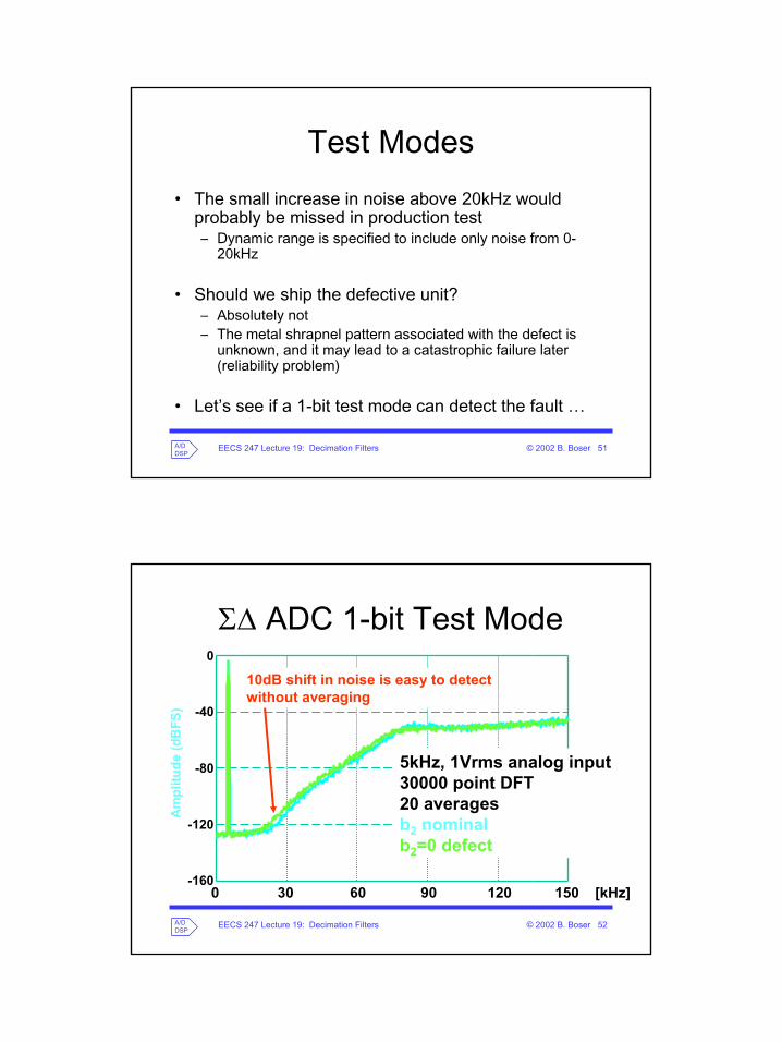
Test Modes• The small increase in noise above 20kHz would
probably be missed in production test– Dynamic range is specified to include only noise from 0-
20kHz
• Should we ship the defective unit?– Absolutely not– The metal shrapnel pattern associated with the defect is
unknown, and it may lead to a catastrophic failure later (reliability problem)
• Let’s see if a 1-bit test mode can detect the fault …
EECS 247 Lecture 19: Decimation Filters © 2002 B. Boser 52A/DDSP
Σ∆ ADC 1-bit Test Mode
Am
plitu
de (d
BFS
)
0
-40
-120
-160
-80
0 120906030 150 [kHz]
5kHz, 1Vrms analog input30000 point DFT20 averagesb2 nominalb2=0 defect
10dB shift in noise is easy to detectwithout averaging
EECS 247 Lecture 19: Decimation Filters © 2002 B. Boser 53A/DDSP
Σ∆ ADC 1-bit Test ModeA
mpl
itude
(dB
FS)
0
-40
-120
-160
-80
0 120906030 150 [kHz]
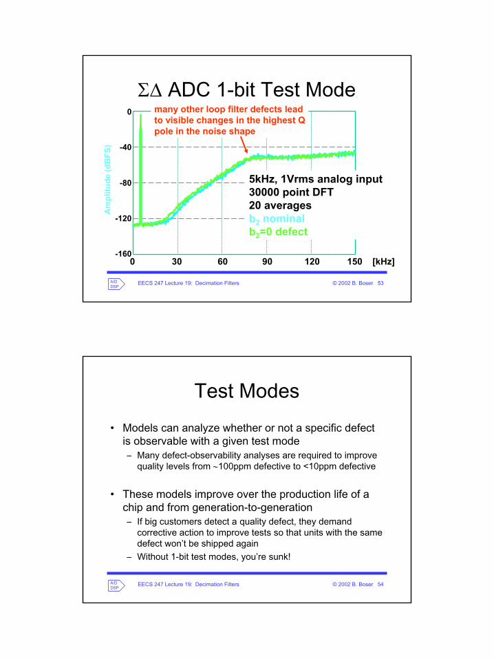
5kHz, 1Vrms analog input30000 point DFT20 averagesb2 nominalb2=0 defect
many other loop filter defects leadto visible changes in the highest Qpole in the noise shape
EECS 247 Lecture 19: Decimation Filters © 2002 B. Boser 54A/DDSP
Test Modes• Models can analyze whether or not a specific defect
is observable with a given test mode– Many defect-observability analyses are required to improve
quality levels from ∼100ppm defective to <10ppm defective
• These models improve over the production life of a chip and from generation-to-generation– If big customers detect a quality defect, they demand
corrective action to improve tests so that units with the same defect won’t be shipped again
– Without 1-bit test modes, you’re sunk!
EECS 247 Lecture 19: Decimation Filters © 2002 B. Boser 55A/DDSP
Multitone Tests
• As long as we’re on the subject of testing, let’s examine a fast, effective method to look at the frequency response of a filter or ADC
– This method is used extensively in production tests of both analog filters and ADCs
– It is not a substitute for classic, fault coverage testing of digital filters
EECS 247 Lecture 19: Decimation Filters © 2002 B. Boser 56A/DDSP
Multitone Tests• IC testers can add sinewaves at many different
frequencies in the digital domain– The digital sum is sent to a test system DAC which
generates the analog input for a device under test– Frequency response at many different input frequencies can
be determined with one test
• Let’s see how our Σ∆ ADC responds to an input which is a sum of 20, 21, 22, 23, 24.375, 25.375, 26.375, and 27.375kHz sinewaves
EECS 247 Lecture 19: Decimation Filters © 2002 B. Boser 57A/DDSP
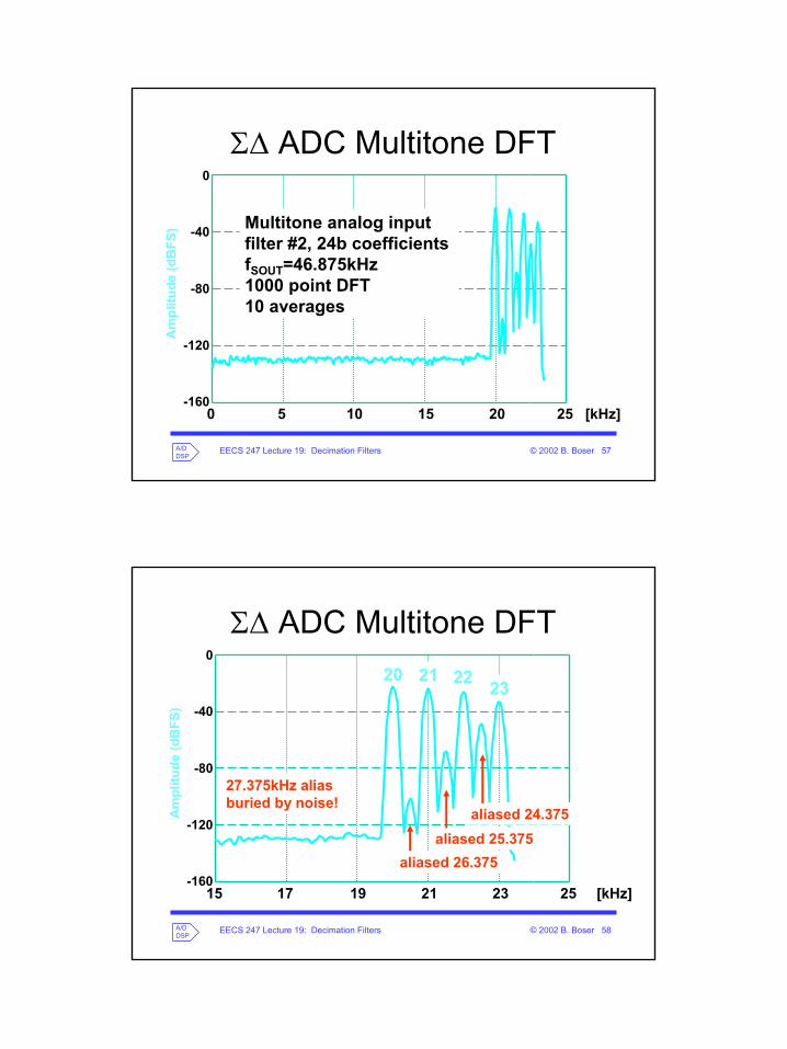
Σ∆ ADC Multitone DFTA
mpl
itude
(dB
FS)
0
-40
-120
-160
-80
0 2015105 25 [kHz]
Multitone analog inputfilter #2, 24b coefficients fSOUT=46.875kHz1000 point DFT10 averages
EECS 247 Lecture 19: Decimation Filters © 2002 B. Boser 58A/DDSP
Σ∆ ADC Multitone DFT
Am
plitu
de (d
BFS
)
0
-40
-120
-160
-80
15 23211917 25 [kHz]
20 21 22 23
aliased 26.375aliased 25.375
aliased 24.375
27.375kHz aliasburied by noise!
EECS 247 Lecture 19: Decimation Filters © 2002 B. Boser 59A/DDSP
Multitone Tests
• Note how elegantly the multitone output amplitudes trace the transition band of the decimation filter
• Total observation time (1000 ADC output samples) must be long enough to resolve each of the individual frequencies– Hz/bin is the reciprocal of the total observation
time
EECS 247 Lecture 19: Decimation Filters © 2002 B. Boser 60A/DDSP
Multistage Decimation Filters• Decimation filter #2 can be realized with a accumulator rate of
57MHz, shift register, and coefficient ROM– Absolutely practical in today’s CMOS processes– A multiplier is not needed
• Multi-rate decimators can achieve the same result with even lower processing cost
• We will:– Illustrate how multistage decimation requires substantially lower
multiply-accumulate rates than single stage decimation– Introduce very specific filter architectures that are specialized just
for decimation/interpolation and can further reduce hardware complexity
EECS 247 Lecture 19: Decimation Filters © 2002 B. Boser 61A/DDSP
Multistage Decimation Filters• In multistage decimation, implement the
sharpest transition bands at the lowest sampling frequency
• For our 3MHz audio modulator, we’ll decimate by 64 in 3 stages– 8X in the first stage– 4X in the second stage– 2X in the third stage
EECS 247 Lecture 19: Decimation Filters © 2002 B. Boser 62A/DDSP
Multistage Decimation Filters• Datapath precision is important here
– Stage 1 has 1-bit input data and doesn’t need a hardware multiplier
– Intermediate rounding operations between stages 1 and 2 and between stages 2 and 3 add quantization noise which must be modeled in a “bit true” fashion
– Final rounding to the 20-bit ADC output adds negligible noise
• Coefficient precision is also important– 24b precision for 135dB stopband attenuation
EECS 247 Lecture 19: Decimation Filters © 2002 B. Boser 63A/DDSP
Parks-McClellan Decimation• In the first pass with synthesize the three
stages with the Parks-McClellan algorithm and stick with floating point numbers– The results provide an estimate of aggregate
multiply accumulate rates
• Each stage will specify 0.0000±0.0033dB ripple from 0-20kHz– Passband ripple in the 3 stages may add– The goal is a “fair” comparison to filter #2
EECS 247 Lecture 19: Decimation Filters © 2002 B. Boser 64A/DDSP
Parks-McClellan Decimation• Stages 1 and 2 prevent decimation from aliasing noise
and tones into frequencies below 27kHz
• Stage 1 stopbands: – 375±27kHz, 750±27kHz, 1125±27kHz, 1473-1500kHz
• Stage 2 stopbands: – 93.75±27kHz, 160.5-187.5kHz
• Stage 3 stopband: 27-46.875kHz
• For each stage we specify 135dB stopband attenuation
EECS 247 Lecture 19: Decimation Filters © 2002 B. Boser 65A/DDSP
Parks-McClellan Decimation• MATLAB’s Parks-McClellan front end doesn’t
handle lowpass filters like stage 1 very easily– The low pass filter we want has a single
passband, multiple stopbands, and interspersed don’t care bands
• We’ll waste zeroes and implement stages 1 and 2 as single-stopband LPFs:– Stage 1 stopband 348-1500kHz– Stage 2 stopband 66.75-187.5kHz– Stage 3 stopband still 27-46.875kHz
EECS 247 Lecture 19: Decimation Filters © 2002 B. Boser 66A/DDSP
Parks-McClellan Decimation• These Parks-McClellan designs yield:
– Stage 1: Length 57 (21.375MHz)– Stage 2: Length 50 (4.688MHz)– Stage 3: Length 84 (3.938MHz)
• Multiply-accumulate rates are shown in redabove– Total multiply-accumulate frequency is 30MHz– Exploiting linear phase coefficient symmetry can
reduce this to 15MHz– The filter #2 design required 57MHz
EECS 247 Lecture 19: Decimation Filters © 2002 B. Boser 67A/DDSP
Parks-McClellan Decimation• Stage 1 uses the most MAC cycles, but it doesn’t
need a hardware multiplier
• DSP conventional wisdom says you should always decimate (or interpolate) in stages– Σ∆ ADC decimation filters with 1-bit inputs are hardly
conventional filters– Both single and multistage designs must be compared in
power and area
• MACs required by unrelated DSP functions may have “free” cycles available for decimation
EECS 247 Lecture 19: Decimation Filters © 2002 B. Boser 68A/DDSP
Manual Decimators• Simple and effective first stage decimators spread
unit circle zeroes evenly in areas where aliasing must be prevented– Start with about 5 zeroes per stopband– Add more if needed to reach –135dB in each band
• Our “manual decimator” requires only Length=38 to achieve specified performance– Zeroes at 350, 360, 370, 380, 390, 400, 726, 738, 750, 762,
764, 1101, 1113, 1125, 1137, 1149, 1476, 1488, and 1500kHz
EECS 247 Lecture 19: Decimation Filters © 2002 B. Boser 69A/DDSP
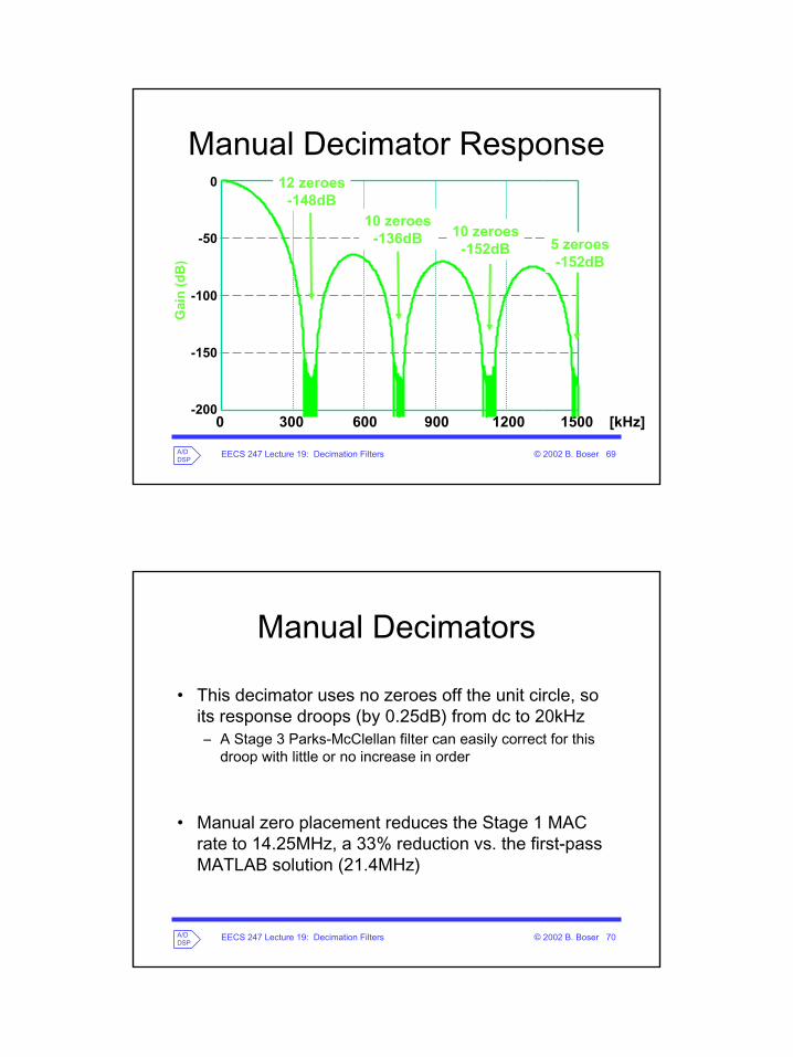
Manual Decimator ResponseG
ain
(dB
)0
-50
-150
-200
-100
0 1200900600300 1500 [kHz]
12 zeroes-148dB
10 zeroes-136dB 10 zeroes
-152dB 5 zeroes-152dB
EECS 247 Lecture 19: Decimation Filters © 2002 B. Boser 70A/DDSP
Manual Decimators
• This decimator uses no zeroes off the unit circle, so its response droops (by 0.25dB) from dc to 20kHz– A Stage 3 Parks-McClellan filter can easily correct for this
droop with little or no increase in order
• Manual zero placement reduces the Stage 1 MAC rate to 14.25MHz, a 33% reduction vs. the first-pass MATLAB solution (21.4MHz)
EECS 247 Lecture 19: Decimation Filters © 2002 B. Boser 71A/DDSP
Clever DecimatorsTwo very clever decimation filter approaches which are occasionally very useful are
• Comb filters– Implement (multiple) zeros on the unit circle very
efficiently
• Half-band filters– For very efficient 2X decimation/interpolation
EECS 247 Lecture 19: Decimation Filters © 2002 B. Boser 72A/DDSP
Comb Filters• Let’s look at the a “rectangular” transfer function,
• This filter has N-1 evenly spaced zeros on the unit circle, except at z=1 LPF
• A N=8 rectangular window is the simplest filter candidate for a decimate-by-8 stage 1 design– Of course, its performance is unimpressive relative to our
Length=38 manual decimator– At least the zeroes are in the right place …
1
7654321
1
0
111
)(
−
−
−−−−−−−
−
=
−
−−
=
++++++++=
= ∑
zz
zzzzzzz
zzH
N
N
i
i
K
EECS 247 Lecture 19: Decimation Filters © 2002 B. Boser 73A/DDSP
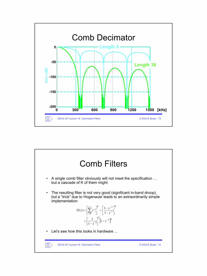
Comb DecimatorG
ain
(dB
)0
-50
-150
-200
-100
0 1200900600300 1500 [kHz]
Length 8
Length 38
EECS 247 Lecture 19: Decimation Filters © 2002 B. Boser 74A/DDSP
• A single comb filter obviously will not meet the specification …but a cascade of K of them might
• The resulting filter is not very good (significant in-band droop), but a “trick” due to Hogenauer leads to an extraordinarily simple implementation
• Let’s see how this looks in hardware …
Comb Filters
[ ]KNK
KNKN
i
i
zz
zzzzH
−−
−
−−
=
−
−
−
=
−−
=
= ∑
111
11)(
1
1
1
0
EECS 247 Lecture 19: Decimation Filters © 2002 B. Boser 75A/DDSP
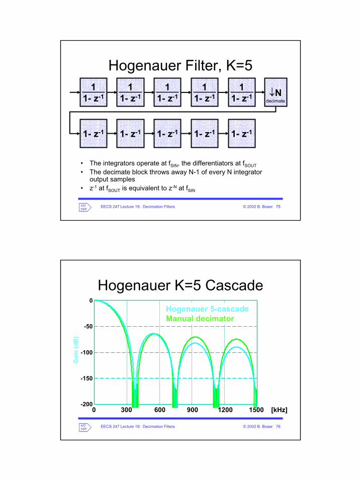
Hogenauer Filter, K=51
1- z-1 ↓Ndecimate
11- z-1
11- z-1
11- z-1
11- z-1
1- z-1 1- z-1 1- z-1 1- z-1 1- z-1
• The integrators operate at fSIN, the differentiators at fSOUT• The decimate block throws away N-1 of every N integrator
output samples• z-1 at fSOUT is equivalent to z-N at fSIN
EECS 247 Lecture 19: Decimation Filters © 2002 B. Boser 76A/DDSP
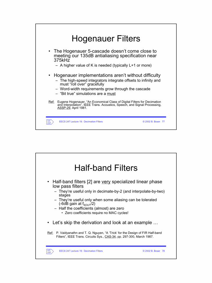
Hogenauer K=5 Cascade
Gai
n (d
B)
0
-50
-150
-200
-100
0 1200900600300 1500 [kHz]
Hogenauer 5-cascadeManual decimator
EECS 247 Lecture 19: Decimation Filters © 2002 B. Boser 77A/DDSP
Hogenauer Filters• The Hogenauer 5-cascade doesn’t come close to
meeting our 135dB antialiasing specification near 375kHz– A higher value of K is needed (typically L+1 or more)
• Hogenauer implementations aren’t without difficulty– The high-speed integrators integrate offsets to infinity and
must “roll over” gracefully– Word-width requirements grow through the cascade– “Bit true” simulations are a must
Ref: Eugene Hogenauer, “An Economical Class of Digital Filters for Decimationand Interpolation”, IEEE Trans. Acoustics, Speech, and Signal Processing, ASSP-29, April 1981.
EECS 247 Lecture 19: Decimation Filters © 2002 B. Boser 78A/DDSP
Half-band Filters• Half-band filters [2] are very specialized linear phase
low pass filters– They’re useful only in decimate-by-2 (and interpolate-by-two)
stages– They’re useful only when some aliasing can be tolerated
(-6dB gain at fSOUT/2)– Half the coefficients (almost) are zero
• Zero coefficients require no MAC cycles!
• Let’s skip the derivation and look at an example …
Ref: P. Vaidyanathn and T. Q. Nguyen, “A ‘Trick’ for the Design of FIR Half-bandFilters”, IEEE Trans. Circuits Sys., CAS-34, pp. 297-300, March 1987.
EECS 247 Lecture 19: Decimation Filters © 2002 B. Boser 79A/DDSP
Half-band Filters• The response of a half-band stage 3 filter F(z) is symmetric
(fSIN=93.75kHz):
– If F(z)’s gain is within 1±ε from 0-20kHz, its gain will be only ε from 26875-46875Hz
• A good audio decimate-by-2 filter
– The half-band filter inherently has –6dB gain at fs/4 = 23437.5Hz
• But how can we get the Park-McClellan algorithm to design a half-band filter? The answer is in ref [2].
• Let’s look at the response …
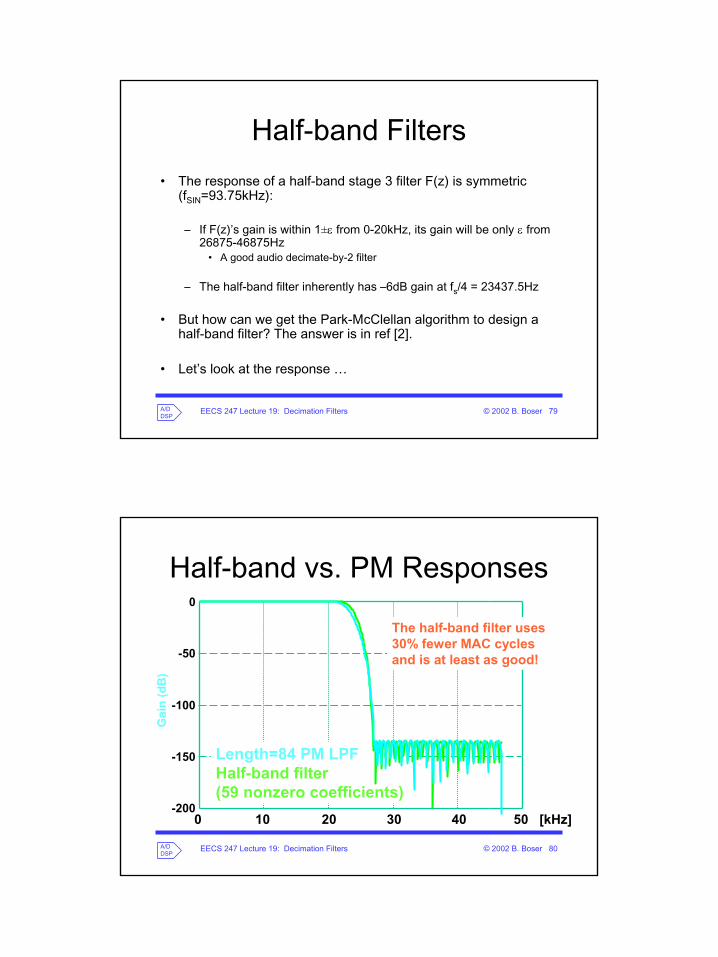
EECS 247 Lecture 19: Decimation Filters © 2002 B. Boser 80A/DDSP
Half-band vs. PM Responses
Gai
n (d
B)
0
-50
-150
-200
-100
0 40302010 50 [kHz]
Length=84 PM LPFHalf-band filter(59 nonzero coefficients)
The half-band filter uses 30% fewer MAC cycles and is at least as good!