Decentralisation and Social Cohesion in Religiously Heterogeneous
24
Convex Optimization — Boyd & Vandenberghe 2. Convex sets • affine and convex sets • some important examples • operations that preserve convexity • generalized inequalities • separating and supporting hyperplanes • dual cones and generalized inequalities 2–1
Transcript of Decentralisation and Social Cohesion in Religiously Heterogeneous
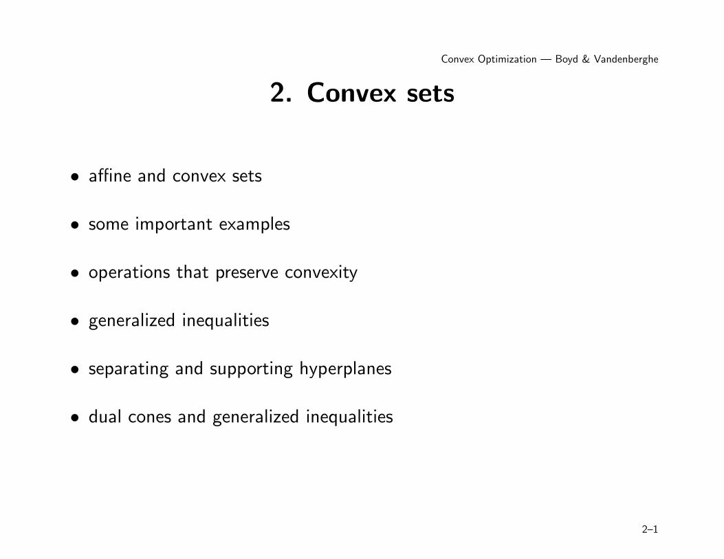
Convex Optimization — Boyd & Vandenberghe
2. Convex sets
• affine and convex sets
• some important examples
• operations that preserve convexity
• generalized inequalities
• separating and supporting hyperplanes
• dual cones and generalized inequalities
2–1
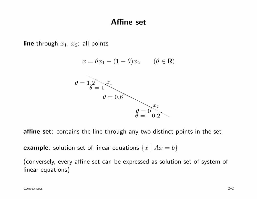
Affine set
line through x1, x2: all points
x = θx1 + (1 − θ)x2 (θ ∈ R)
θ = 1.2 x1θ = 1
θ = 0.6
x2 θ = 0 θ = −0.2
affine set: contains the line through any two distinct points in the set
example: solution set of linear equations {x | Ax = b}
(conversely, every affine set can be expressed as solution set of system oflinear equations)
Convex sets 2–2
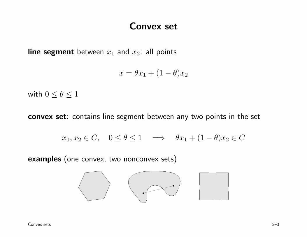
Convex set
line segment between x1 and x2: all points
x = θx1 + (1 − θ)x2
with 0 ≤ θ ≤ 1
convex set: contains line segment between any two points in the set
x1, x2 ∈ C, 0 ≤ θ ≤ 1 =⇒ θx1 + (1 − θ)x2 ∈ C
examples (one convex, two nonconvex sets)
Convex sets 2–3
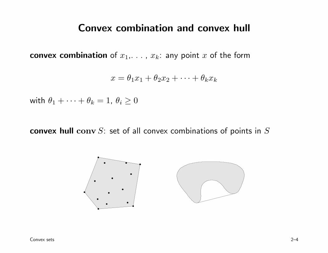
Convex combination and convex hull
convex combination of x1,. . . , xk: any point x of the form
x = θ1x1 + θ2x2 + · · · + θkxk
with θ1 + · · · + θk = 1, θi ≥ 0
convex hull conv S: set of all convex combinations of points in S
Convex sets 2–4
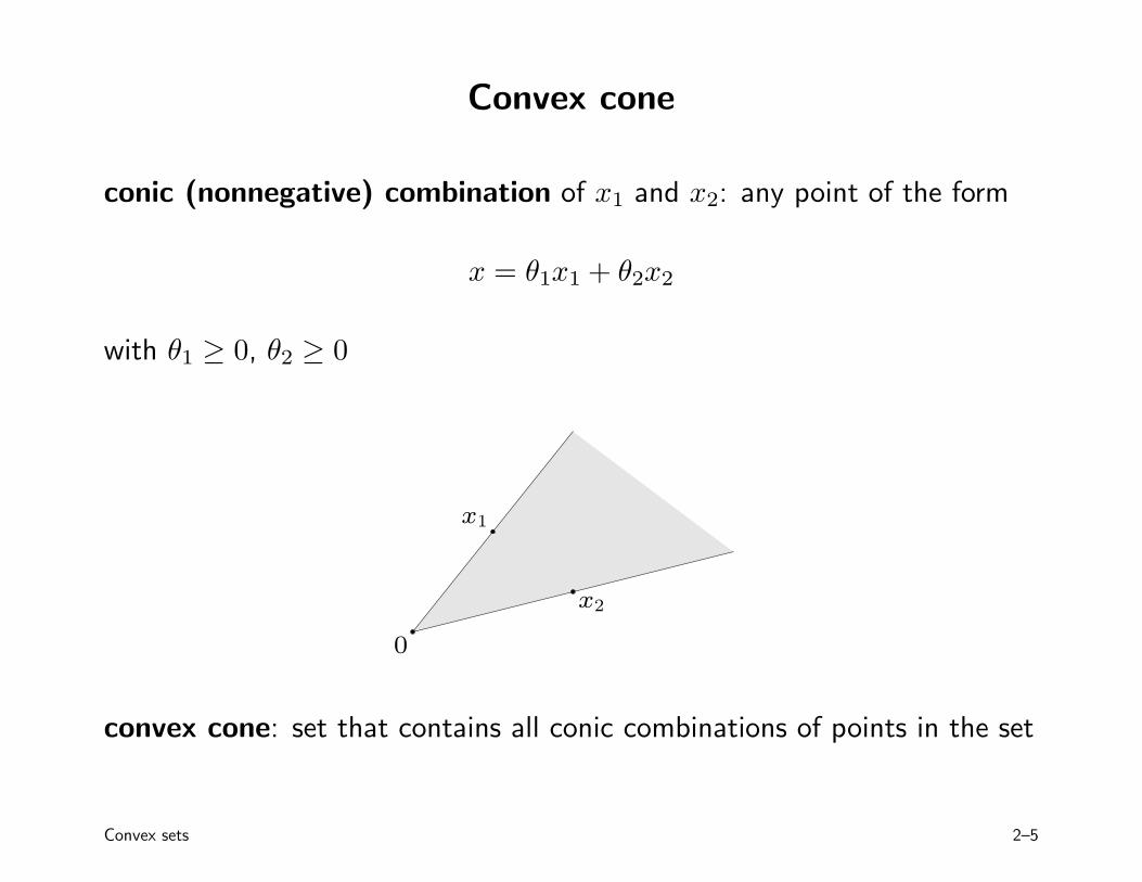
Convex cone
conic (nonnegative) combination of x1 and x2: any point of the form
x = θ1x1 + θ2x2
with θ1 ≥ 0, θ2 ≥ 0
0
x1
x2
convex cone: set that contains all conic combinations of points in the set
Convex sets 2–5
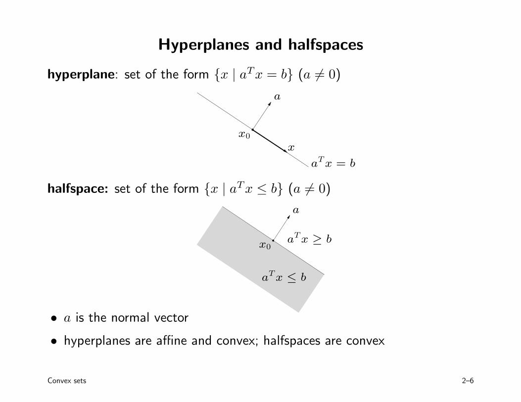
Hyperplanes and halfspaces
hyperplane: set of the form {x | aTx = b} (a = 0� )
a
x0
x
aTx = b
halfspace: set of the form {x | aT �x ≤ b} (a = 0)
a
a T x ≥ b
a T x ≤ b
x0
• a is the normal vector
• hyperplanes are affine and convex; halfspaces are convex
Convex sets 2–6
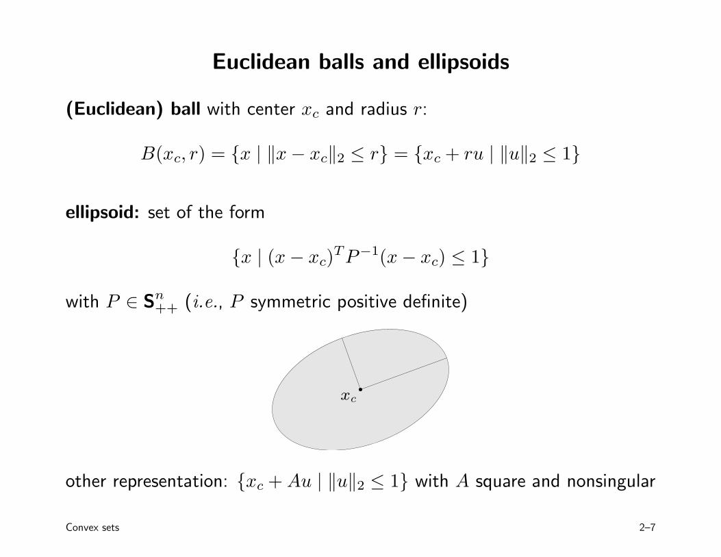
Euclidean balls and ellipsoids
(Euclidean) ball with center xc and radius r:
B(xc, r) = {x | �x − xc�2 ≤ r} = {xc + ru | �u�2 ≤ 1}
ellipsoid: set of the form
{x | (x − xc)TP−1(x − xc) ≤ 1}
with P ∈ Sn (i.e., P symmetric positive definite) ++
xc
other representation: {xc + Au | �u�2 ≤ 1} with A square and nonsingular
Convex sets 2–7
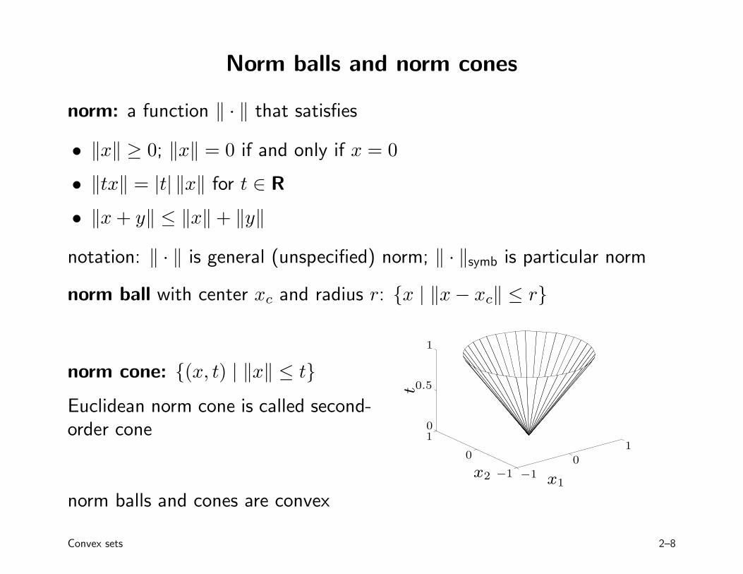
Norm balls and norm cones
norm: a function � · � that satisfies
• �x� ≥ 0; �x� = 0 if and only if x = 0
• �tx� = |t| �x� for t ∈ R
• �x + y� ≤ �x� + �y�
notation: � · � is general (unspecified) norm; � · �symb is particular norm
norm ball with center xc and radius r: {x | �x − xc� ≤ r}
1
norm cone: {(x, t) | �x� ≤ t} 0.5
Euclidean norm cone is called second-order cone 1
0
1 0 0 x2 −1 −1 x1
t
norm balls and cones are convex
Convex sets 2–8
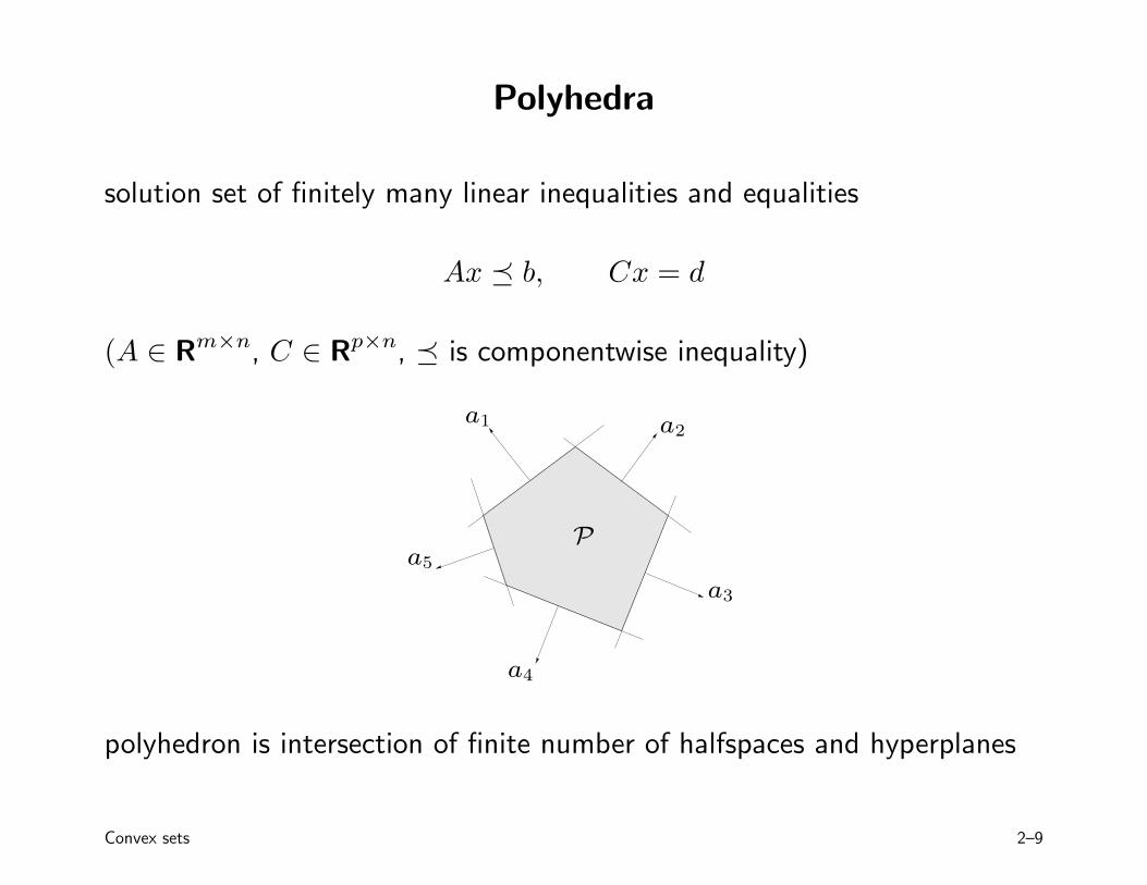
Polyhedra
solution set of finitely many linear inequalities and equalities
Ax � b, Cx = d
(A ∈ Rm×n , C ∈ Rp×n , � is componentwise inequality)
a1
a5
a2
a4
P
a3
polyhedron is intersection of finite number of halfspaces and hyperplanes
Convex sets 2–9
� �
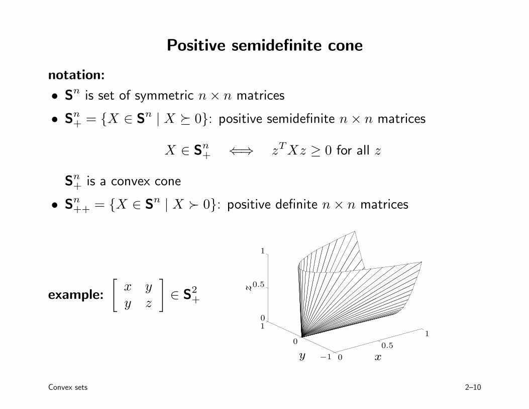
Positive semidefinite cone
notation:
• Sn is set of symmetric n × n matrices
• S+ n = {X ∈ Sn | X � 0}: positive semidefinite n × n matrices
X ∈ Sn ⇐⇒ z TXz ≥ 0 for all z+
Sn is a convex cone +
• S++ n = {X ∈ Sn | X ≻ 0}: positive definite n × n matrices
1
example: x y
∈ S20.5
+y z 0
z
1 1
0 0.5
y −1 0 x
Convex sets 2–10
Operations that preserve convexity
practical methods for establishing convexity of a set C
1. apply definition
x1, x2 ∈ C, 0 ≤ θ ≤ 1 =⇒ θx1 + (1 − θ)x2 ∈ C
2. show that C is obtained from simple convex sets (hyperplanes, halfspaces, norm balls, . . . ) by operations that preserve convexity
• intersection • affine functions • perspective function • linear-fractional functions
Convex sets 2–11
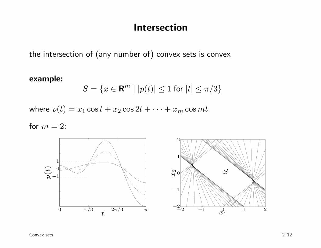
Intersection
the intersection of (any number of) convex sets is convex
example: S = {x ∈ Rm | |p(t)| ≤ 1 for |t| ≤ π/3}
where p(t) = x1 cos t + x2 cos 2t + · · · + xm cos mt
for m = 2:
2
1 1
S
−2 −1 0 1 2
0
0 π/3 2π/3 π
x2
p(t
)
−10
−1
−2
t x1
Convex sets 2–12
Affine function
suppose f : Rn → Rm is affine (f(x) = Ax + b with A ∈ Rm×n , b ∈ Rm)
• the image of a convex set under f is convex
S ⊆ Rn convex =⇒ f(S) = {f(x) | x ∈ S} convex
• the inverse image f−1(C) of a convex set under f is convex
C ⊆ Rm convex =⇒ f−1(C) = {x ∈ Rn | f(x) ∈ C} convex
examples
• scaling, translation, projection
• solution set of linear matrix inequality {x | x1A1 + · · · + xmAm � B} (with Ai, B ∈ Sp)
• hyperbolic cone {x | xTPx ≤ (cTx)2, cTx ≥ 0} (with P ∈ Sn )+
Convex sets 2–13
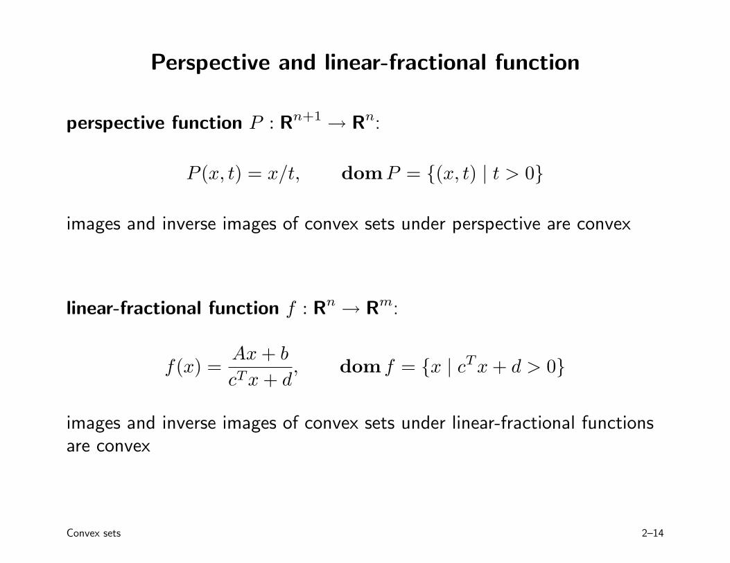
Perspective and linear-fractional function
perspective function P : Rn+1 → Rn:
P (x, t) = x/t, dom P = {(x, t) | t > 0}
images and inverse images of convex sets under perspective are convex
linear-fractional function f : Rn → Rm:
f(x) = Ax + b
, dom f = {x | c T x + d > 0} cTx + d
images and inverse images of convex sets under linear-fractional functions are convex
Convex sets 2–14
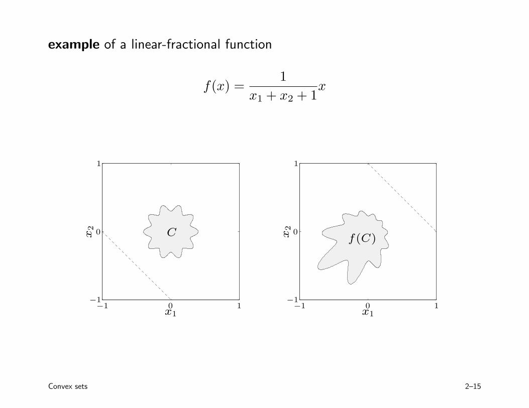
example of a linear-fractional function
1 f(x) = x
x1 + x2 + 1
1 1
f(C)Cx2
x2
0 0
−1 −1 −1 0 1 −1 0 1
x1 x1
Convex sets 2–15
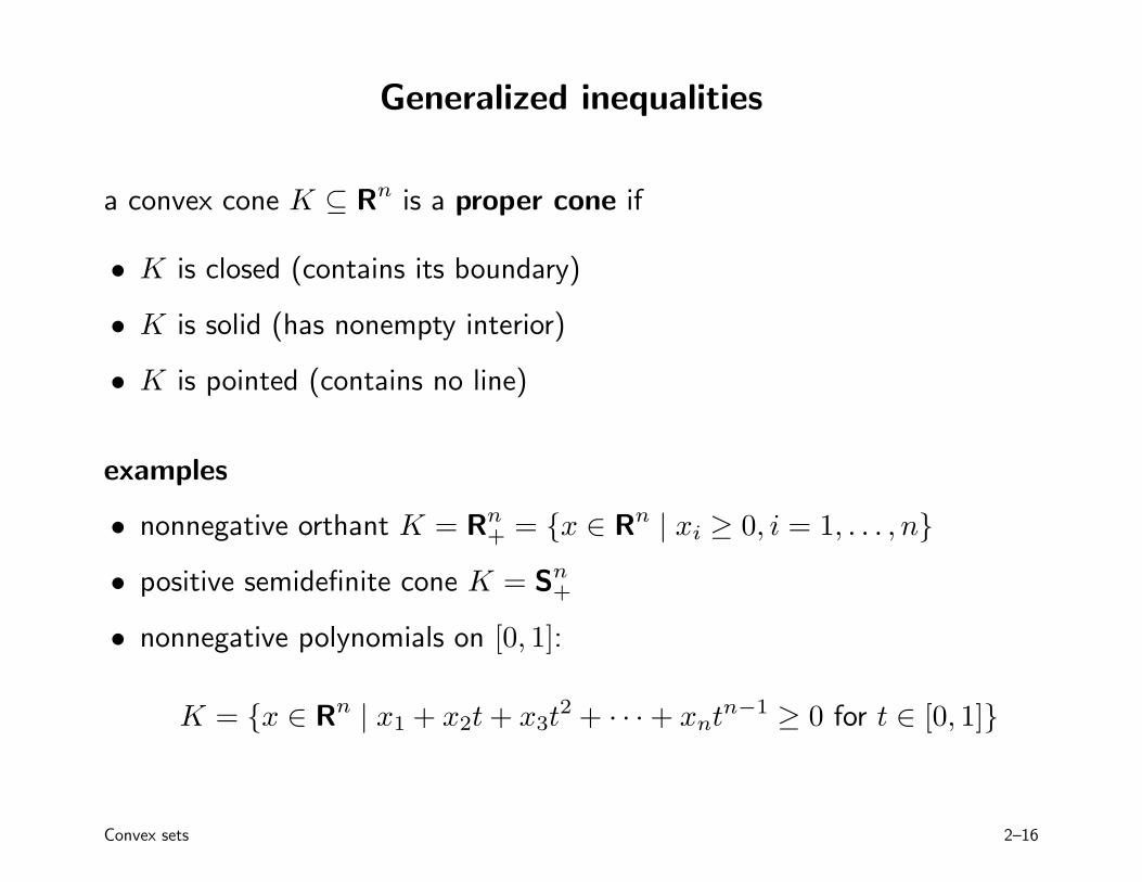
Generalized inequalities
a convex cone K ⊆ Rn is a proper cone if
• K is closed (contains its boundary)
• K is solid (has nonempty interior)
• K is pointed (contains no line)
examples
• nonnegative orthant K = Rn = {x ∈ Rn | xi ≥ 0, i = 1, . . . , n}+
• positive semidefinite cone K = Sn +
• nonnegative polynomials on [0, 1]:
K = {x ∈ Rn | x1 + x2t + x3t2 + · · · + xntn−1 ≥ 0 for t ∈ [0, 1]}
Convex sets 2–16
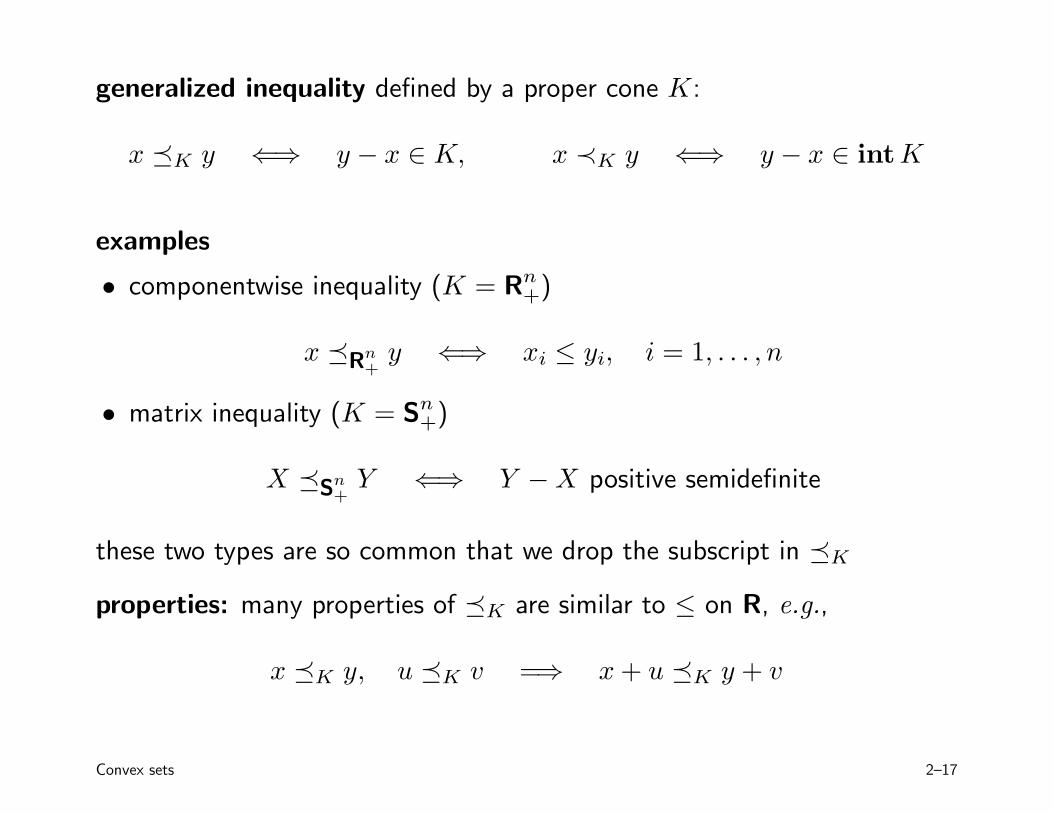
generalized inequality defined by a proper cone K:
x �K y ⇐⇒ y − x ∈ K, x ≺K y ⇐⇒ y − x ∈ int K
examples
= Rn +• componentwise inequality (K )
x �Rn
• matrix inequality (K = Sn +
+y ⇐⇒ xi ≤ yi, i = 1, . . . , n
)
X �Sn
these two types are so common that we drop the subscript in �K
properties: many properties of �K are similar to ≤ on R, e.g.,
x �K y, u �K v =⇒ x + u �K y + v
+ Y ⇐⇒ Y − X positive semidefinite
Convex sets 2–17
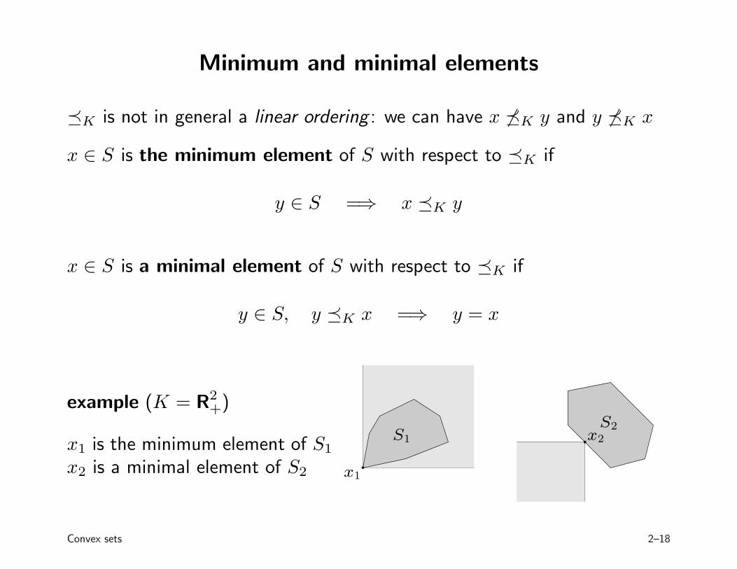
Minimum and minimal elements
�K is not in general a linear ordering : we can have x ��K y and y ��K x
x ∈ S is the minimum element of S with respect to �K if
y ∈ S =⇒ x �K y
x ∈ S is a minimal element of S with respect to �K if
y ∈ S, y �K x =⇒ y = x
example (K = R+2 )
x1 is the minimum element of S1
x2 is a minimal element of S2 x1
x2S1 S2
Convex sets 2–18
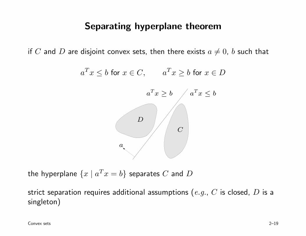
Separating hyperplane theorem
if C and D are disjoint convex sets, then there exists a �= 0, b such that
a T x ≤ b for x ∈ C, a T x ≥ b for x ∈ D
aTx ≥ b aTx ≤ b
a
D
C
the hyperplane {x | aTx = b} separates C and D
strict separation requires additional assumptions (e.g., C is closed, D is a singleton)
Convex sets 2–19
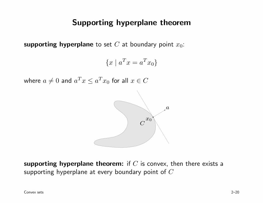
Supporting hyperplane theorem
supporting hyperplane to set C at boundary point x0:
{x | a T x = a T x0}
where a � Tx ≤ Tx0 for all x ∈ C= 0 and a a
C
a
x0
supporting hyperplane theorem: if C is convex, then there exists a supporting hyperplane at every boundary point of C
Convex sets 2–20
Dual cones and generalized inequalities
dual cone of a cone K:
K ∗ = {y | y T x ≥ 0 for all x ∈ K}
examples
• K = Rn : K∗ = Rn + +
• K = Sn : K∗ = Sn + +
• K = {(x, t) | �x�2 ≤ t}: K∗ = {(x, t) | �x�2 ≤ t}
• K = {(x, t) | �x�1 ≤ t}: K∗ = {(x, t) | �x�∞ ≤ t}
first three examples are self-dual cones
dual cones of proper cones are proper, hence define generalized inequalities:
y �K∗ 0 ⇐⇒ y T x ≥ 0 for all x �K 0
Convex sets 2–21
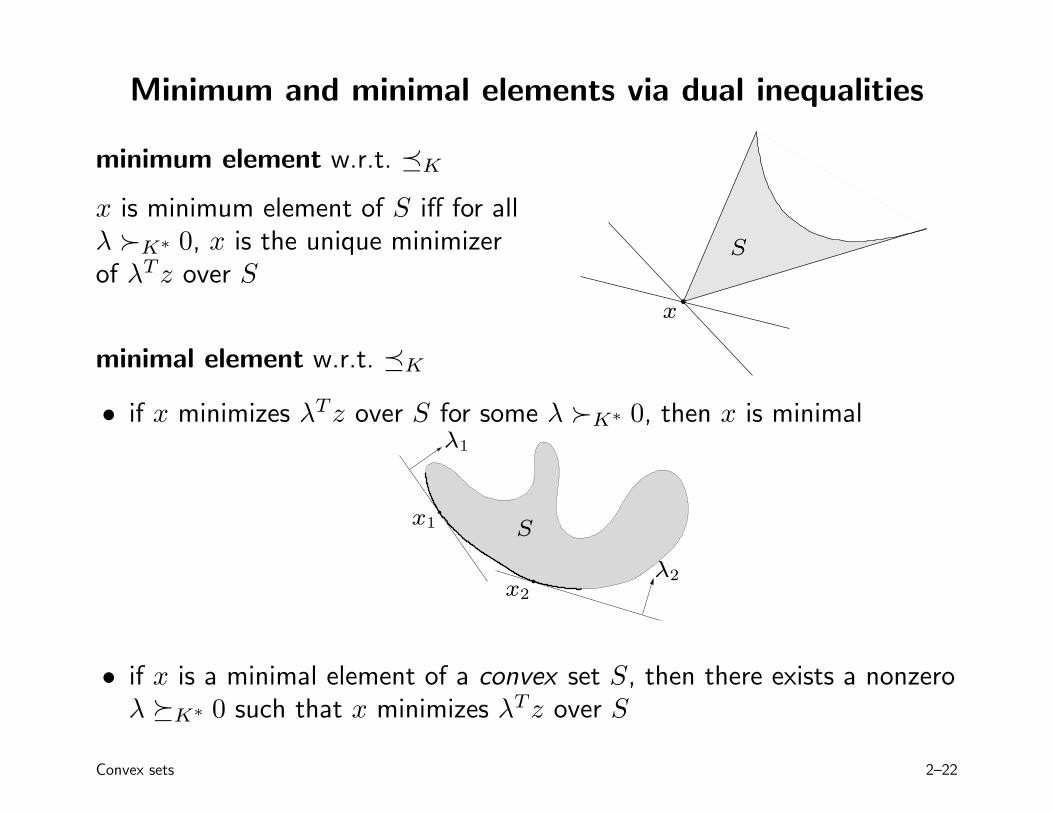
Minimum and minimal elements via dual inequalities
minimum element w.r.t. �K
x is minimum element of S iff for all λ ≻K∗ 0, x is the unique minimizer of λTz over S
minimal element w.r.t. �K
• if x minimizes λTz over S for some λ ≻K∗ 0, then x is minimal
x
S
Sx1
x2
λ1
λ2
• if x is a minimal element of a convex set S, then there exists a nonzero λ �K∗ 0 such that x minimizes λTz over S
Convex sets 2–22
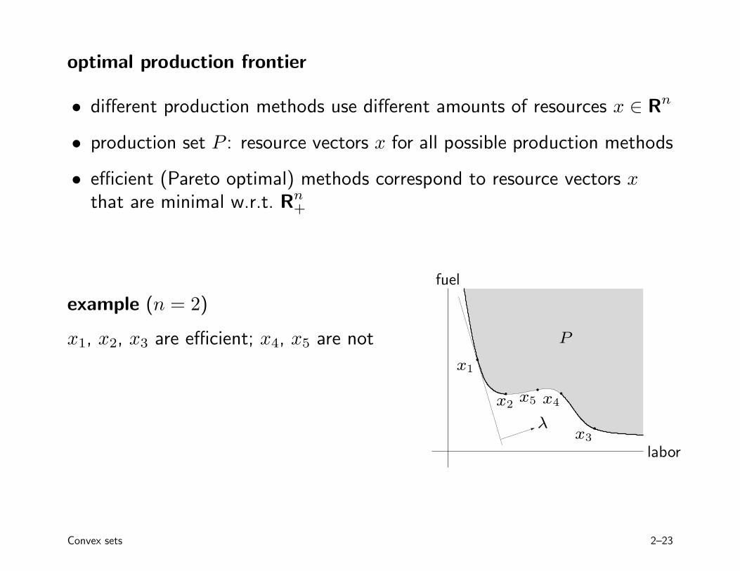
optimal production frontier
• different production methods use different amounts of resources x ∈ Rn
• production set P : resource vectors x for all possible production methods
• efficient (Pareto optimal) methods correspond to resource vectors x that are minimal w.r.t. Rn
+
fuel
example (n = 2)
x1, x2, x3 are efficient; x4, x5 are not
x3
x2 x5 x4
x1
λ
P
labor
Convex sets 2–23

MIT OpenCourseWare http://ocw.mit.edu
6.079 / 6.975 Introduction to Convex Optimization Fall 2009
For information about citing these materials or our Terms of Use, visit: http://ocw.mit.edu/terms.