Dataflow Analysis Frameworksaldrich/courses/654-sp07/slides/...1 Analysis of Software Artifacts -...
28
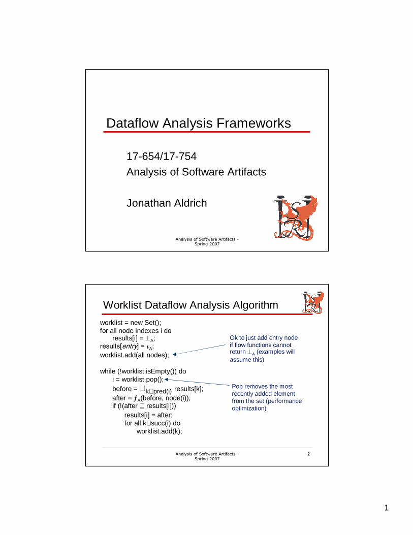
1 Analysis of Software Artifacts - Spring 2007 1 Dataflow Analysis Frameworks 17-654/17-754 Analysis of Software Artifacts Jonathan Aldrich Analysis of Software Artifacts - Spring 2007 2 Worklist Dataflow Analysis Algorithm worklist = new Set(); for all node indexes i do results[i] = ⊥ A ; results[entry] = ι A ; worklist.add(all nodes); while (!worklist.isEmpty()) do i = worklist.pop(); before = ⊔ k∈pred(i) results[k]; after = ƒ A (before, node(i)); if (!(after ⊑ results[i])) results[i] = after; for all k∈succ(i) do worklist.add(k); Ok to just add entry node if flow functions cannot return ⊥ A (examples will assume this) Pop removes the most recently added element from the set (performance optimization)
Transcript of Dataflow Analysis Frameworksaldrich/courses/654-sp07/slides/...1 Analysis of Software Artifacts -...
1
Analysis of Software Artifacts -Spring 2007
1
Dataflow Analysis Frameworks
17-654/17-754Analysis of Software Artifacts
Jonathan Aldrich
Analysis of Software Artifacts -Spring 2007
2
Worklist Dataflow Analysis Algorithm
worklist = new Set();for all node indexes i do
results[i] = ⊥A;results[entry] = ιA;worklist.add(all nodes);
while (!worklist.isEmpty()) doi = worklist.pop();before = ⊔k∈pred(i) results[k];after = ƒA(before, node(i));if (!(after ⊑ results[i]))
results[i] = after;for all k∈succ(i) do
worklist.add(k);
Ok to just add entry node if flow functions cannot return ⊥A (examples will assume this)
Pop removes the most recently added element from the set (performance optimization)
2
Analysis of Software Artifacts -Spring 2007
3
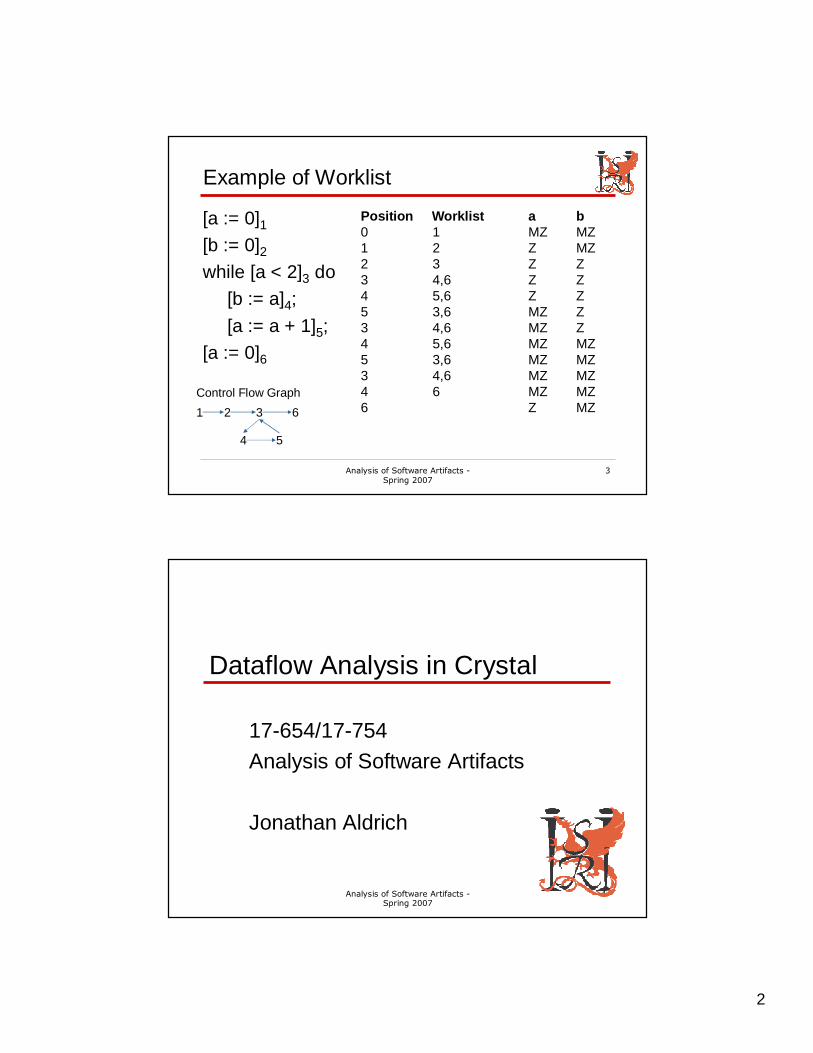
Example of Worklist
[a := 0]1[b := 0]2while [a < 2]3 do
[b := a]4;
[a := a + 1]5;
[a := 0]6
Position Worklist a b0 1 MZ MZ1 2 Z MZ2 3 Z Z3 4,6 Z Z4 5,6 Z Z5 3,6 MZ Z3 4,6 MZ Z4 5,6 MZ MZ5 3,6 MZ MZ3 4,6 MZ MZ4 6 MZ MZ6 Z MZ1 2 3
4 5
6
Control Flow Graph
Analysis of Software Artifacts -Spring 2007
4
Dataflow Analysis in Crystal
17-654/17-754Analysis of Software Artifacts
Jonathan Aldrich
3
Analysis of Software Artifacts -Spring 2007
5
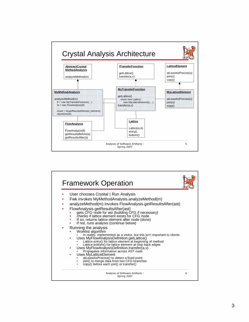
Crystal Analysis Architecture
ITransferFunction
getLattice()transfer(a,v)
FlowAnalysis
FlowAnalysis(tf)getResultsBefore(a)getResultsAfter(a)
AbstractCrystalMethodAnalysis
analyzeMethod(m)
MyMethodAnalysis
analyzeMethod(m)tf = new MyTransferFunction(…)fa = new FlowAnalysis(tf);…result = fa.getResultsAfter(ast_element);report(result);
Lattice
Lattice(e,b)entry()bottom()
MyTransferFunction
getLattice()return new Lattice(
new MyLatticeElement(),…)transfer(a,v)
….
LatticeElement
atLeastAsPrecise(o)join(o)copy()
MyLatticeElement
atLeastAsPrecise(o)join(o)copy()
Analysis of Software Artifacts -Spring 2007
6
Framework Operation• User chooses Crystal | Run Analysis• Fwk invokes MyMethodAnalysis.analyzeMethod(m)• analyzeMethod(m) invokes FlowAnalysis.getResultsAfter(ast)• FlowAnalysis.getResultsAfter(ast)
• gets CFG node for ast (building CFG if necessary)• checks if lattice element exists for CFG node• If so, returns lattice element after node (done)• If not, runs analysis (continue below)
• Running the analysis• Worklist algorithm
• In reality, implemented as a visitor, but this isn’t important to clients• Uses MyFlowAnalysisDefinition.getLattice()
• Lattice.entry() for lattice element at beginning of method• Lattice.bottom() for lattice element at loop back edges
• Uses MyFlowAnalysisDefinition.transfer(a,v)• Propagates information across AST node
• Uses MyLatticeElement• atLeastAsPrecise() to detect a fixed point• join() to merge data from two CFG branches• copy() before each join() or transfer()
4
Analysis of Software Artifacts -Spring 2007
7
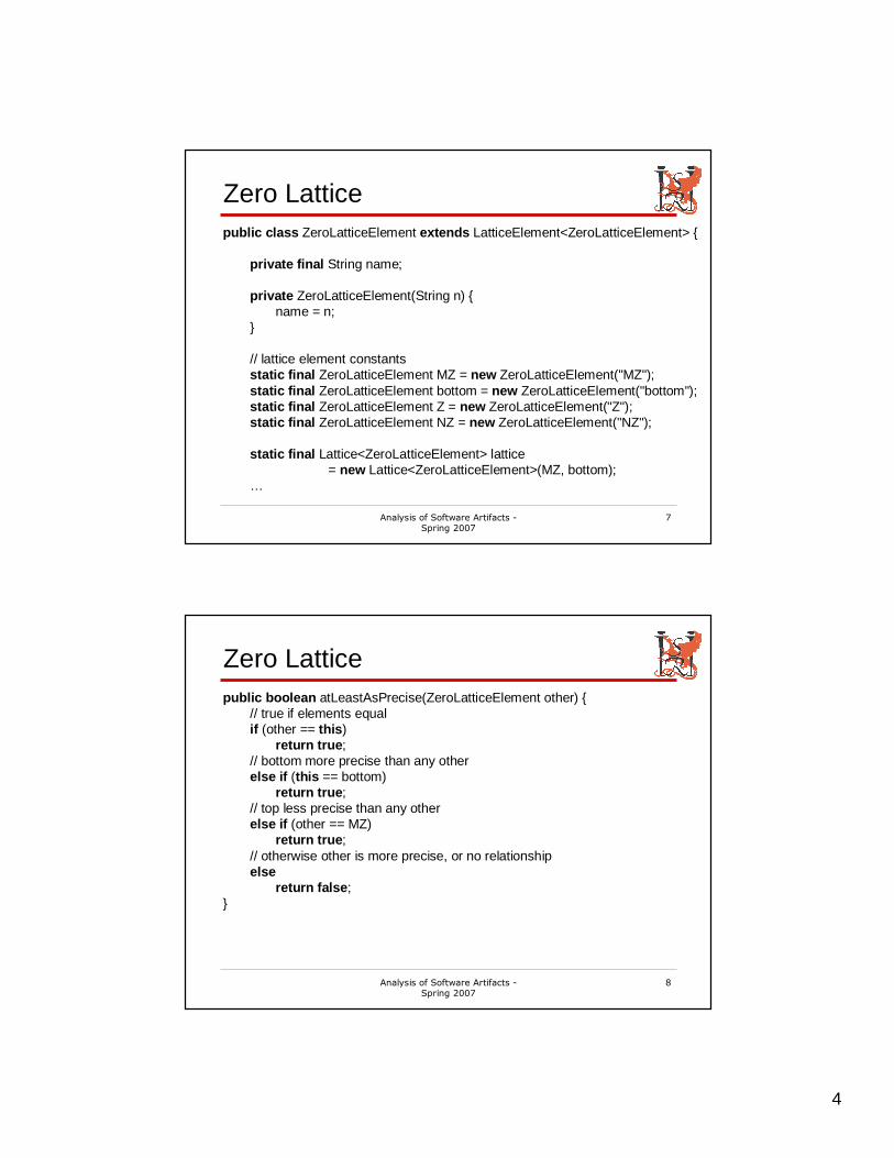
Zero Latticepublic class ZeroLatticeElement extends LatticeElement<ZeroLatticeElement> {
private final String name;
private ZeroLatticeElement(String n) {name = n;
}
// lattice element constantsstatic final ZeroLatticeElement MZ = new ZeroLatticeElement("MZ");static final ZeroLatticeElement bottom = new ZeroLatticeElement("bottom");static final ZeroLatticeElement Z = new ZeroLatticeElement("Z");static final ZeroLatticeElement NZ = new ZeroLatticeElement("NZ");
static final Lattice<ZeroLatticeElement> lattice= new Lattice<ZeroLatticeElement>(MZ, bottom);
…
Analysis of Software Artifacts -Spring 2007
8
Zero Latticepublic boolean atLeastAsPrecise(ZeroLatticeElement other) {
// true if elements equalif (other == this)
return true;// bottom more precise than any otherelse if (this == bottom)
return true;// top less precise than any otherelse if (other == MZ)
return true;// otherwise other is more precise, or no relationshipelse
return false;}
5
Analysis of Software Artifacts -Spring 2007
9
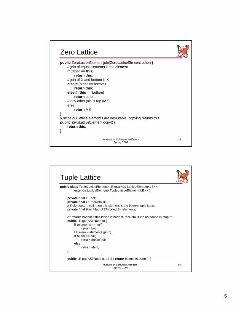
Zero Latticepublic ZeroLatticeElement join(ZeroLatticeElement other) {
// join of equal elements is the elementif (other == this)
return this;// join of X and bottom is Xelse if (other == bottom)
return this;else if (this == bottom)
return other;// any other join is top (MZ)else
return MZ;}// since our lattice elements are immutable, copying returns thispublic ZeroLatticeElement copy() {
return this;}
Analysis of Software Artifacts -Spring 2007
10
Tuple Latticepublic class TupleLatticeElement<LE extends LatticeElement<LE>>
extends LatticeElement<TupleLatticeElement<LE>> {
private final LE bot;private final LE theDefault;// if elements==null, then this element is the bottom tuple lattice private final HashMap<ASTNode,LE> elements;
/** returns bottom if this lattice is bottom, theDefault if n not found in map */public LE get(ASTNode n) {
if (elements == null)return bot;
LE elem = elements.get(n);if (elem == null)
return theDefault;else
return elem;}
public LE put(ASTNode n, LE l) { return elements.put(n,l); }
6
Analysis of Software Artifacts -Spring 2007
11
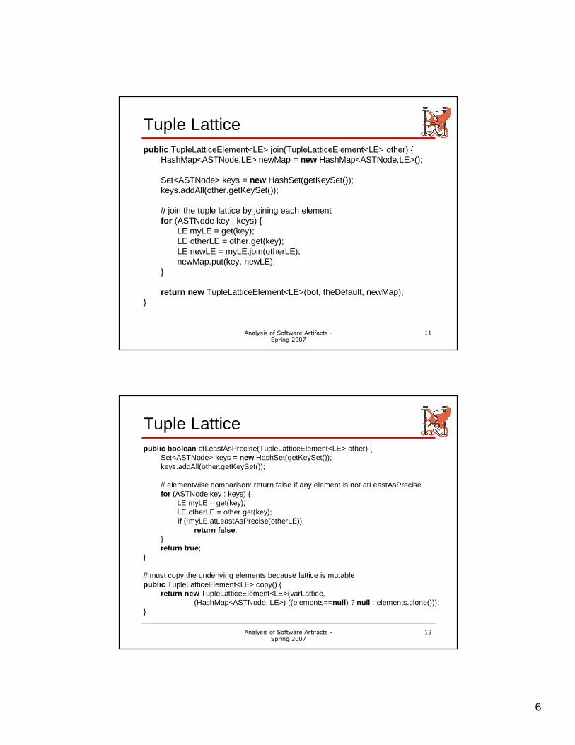
Tuple Latticepublic TupleLatticeElement<LE> join(TupleLatticeElement<LE> other) {
HashMap<ASTNode,LE> newMap = new HashMap<ASTNode,LE>();
Set<ASTNode> keys = new HashSet(getKeySet());keys.addAll(other.getKeySet());
// join the tuple lattice by joining each elementfor (ASTNode key : keys) {
LE myLE = get(key);LE otherLE = other.get(key);LE newLE = myLE.join(otherLE);newMap.put(key, newLE);
}
return new TupleLatticeElement<LE>(bot, theDefault, newMap);}
Analysis of Software Artifacts -Spring 2007
12
Tuple Latticepublic boolean atLeastAsPrecise(TupleLatticeElement<LE> other) {
Set<ASTNode> keys = new HashSet(getKeySet());keys.addAll(other.getKeySet());
// elementwise comparison: return false if any element is not atLeastAsPrecisefor (ASTNode key : keys) {
LE myLE = get(key);LE otherLE = other.get(key);if (!myLE.atLeastAsPrecise(otherLE))
return false;}return true;
}
// must copy the underlying elements because lattice is mutablepublic TupleLatticeElement<LE> copy() {
return new TupleLatticeElement<LE>(varLattice,(HashMap<ASTNode, LE>) ((elements==null) ? null : elements.clone()));
}
7
Analysis of Software Artifacts -Spring 2007
13
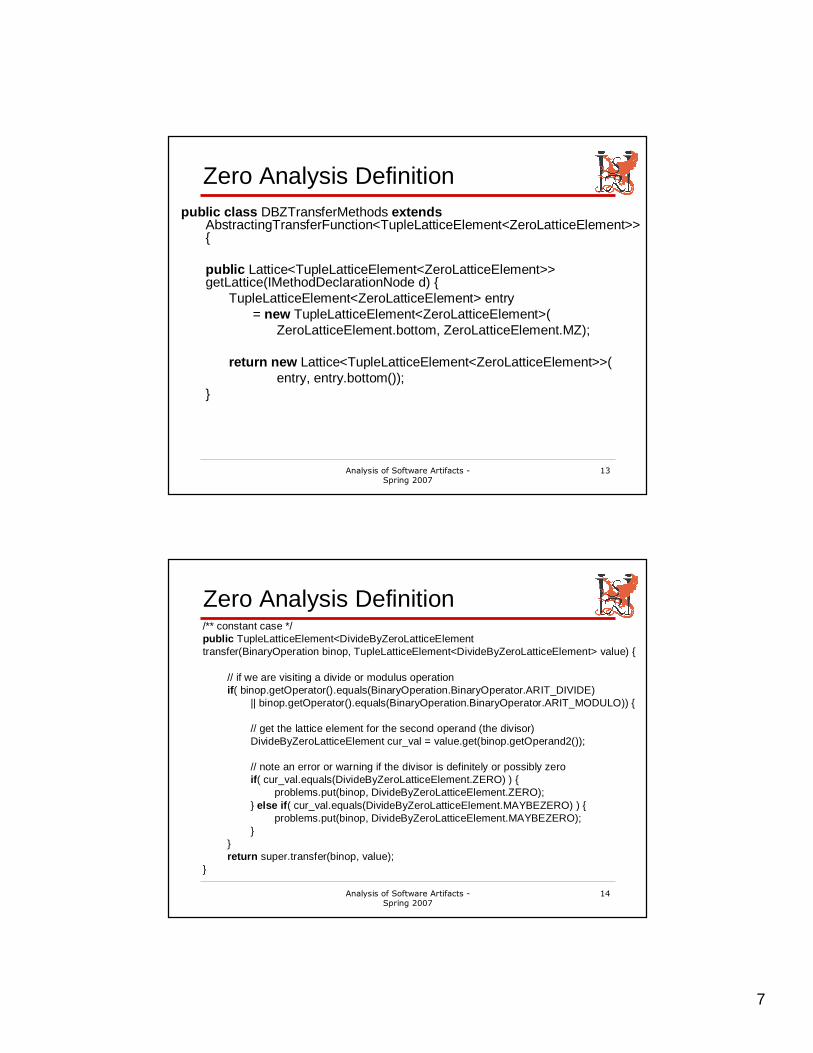
Zero Analysis Definitionpublic class DBZTransferMethods extends
AbstractingTransferFunction<TupleLatticeElement<ZeroLatticeElement>> {
public Lattice<TupleLatticeElement<ZeroLatticeElement>> getLattice(IMethodDeclarationNode d) {
TupleLatticeElement<ZeroLatticeElement> entry= new TupleLatticeElement<ZeroLatticeElement>(
ZeroLatticeElement.bottom, ZeroLatticeElement.MZ);
return new Lattice<TupleLatticeElement<ZeroLatticeElement>>(entry, entry.bottom());
}
Analysis of Software Artifacts -Spring 2007
14
Zero Analysis Definition/** constant case */public TupleLatticeElement<DivideByZeroLatticeElementtransfer(BinaryOperation binop, TupleLatticeElement<DivideByZeroLatticeElement> value) {
// if we are visiting a divide or modulus operationif( binop.getOperator().equals(BinaryOperation.BinaryOperator.ARIT_DIVIDE)
|| binop.getOperator().equals(BinaryOperation.BinaryOperator.ARIT_MODULO)) {
// get the lattice element for the second operand (the divisor)DivideByZeroLatticeElement cur_val = value.get(binop.getOperand2());
// note an error or warning if the divisor is definitely or possibly zeroif( cur_val.equals(DivideByZeroLatticeElement.ZERO) ) {
problems.put(binop, DivideByZeroLatticeElement.ZERO);} else if( cur_val.equals(DivideByZeroLatticeElement.MAYBEZERO) ) {
problems.put(binop, DivideByZeroLatticeElement.MAYBEZERO);}
}return super.transfer(binop, value);
}
8
Analysis of Software Artifacts -Spring 2007
15
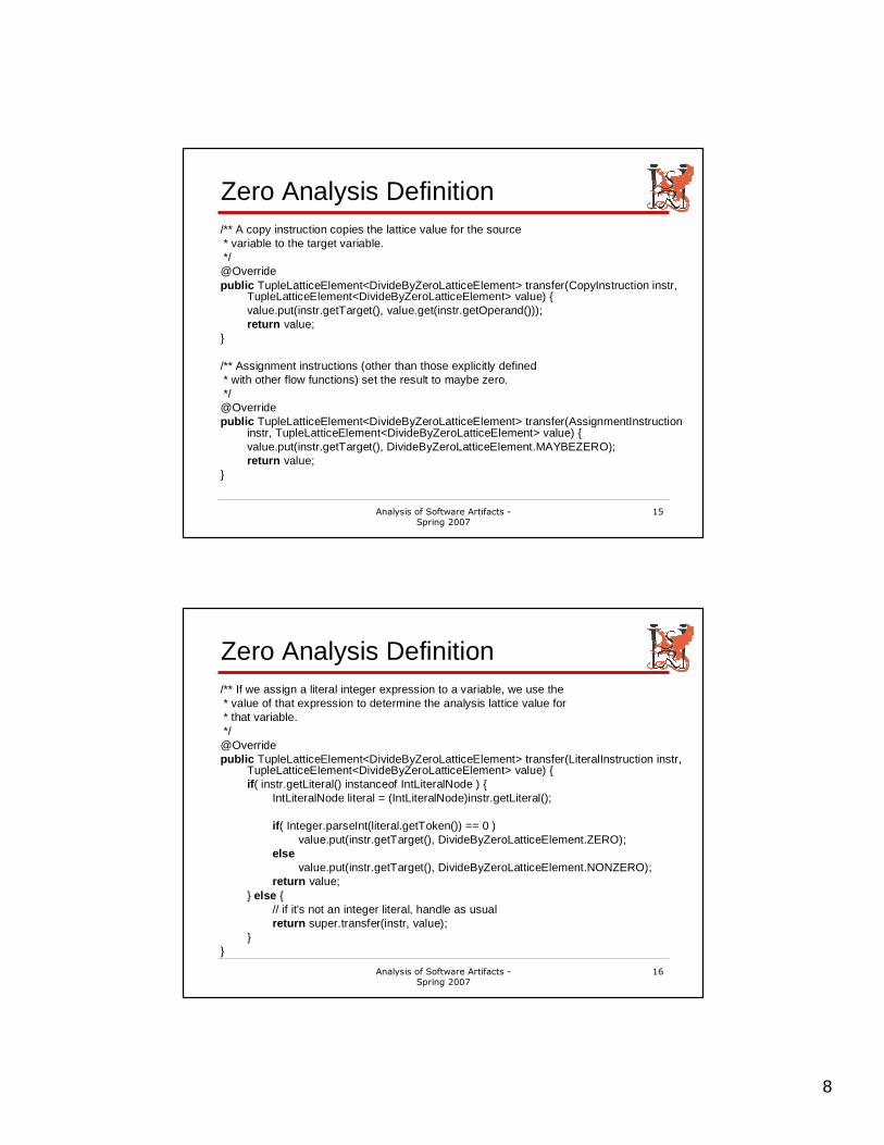
Zero Analysis Definition/** A copy instruction copies the lattice value for the source* variable to the target variable.*/@Overridepublic TupleLatticeElement<DivideByZeroLatticeElement> transfer(CopyInstruction instr,
TupleLatticeElement<DivideByZeroLatticeElement> value) {value.put(instr.getTarget(), value.get(instr.getOperand()));return value;
}
/** Assignment instructions (other than those explicitly defined* with other flow functions) set the result to maybe zero.*/@Overridepublic TupleLatticeElement<DivideByZeroLatticeElement> transfer(AssignmentInstruction
instr, TupleLatticeElement<DivideByZeroLatticeElement> value) {value.put(instr.getTarget(), DivideByZeroLatticeElement.MAYBEZERO);return value;
}
Analysis of Software Artifacts -Spring 2007
16
Zero Analysis Definition/** If we assign a literal integer expression to a variable, we use the* value of that expression to determine the analysis lattice value for* that variable.*/ @Overridepublic TupleLatticeElement<DivideByZeroLatticeElement> transfer(LiteralInstruction instr,
TupleLatticeElement<DivideByZeroLatticeElement> value) {if( instr.getLiteral() instanceof IntLiteralNode ) {
IntLiteralNode literal = (IntLiteralNode)instr.getLiteral();
if( Integer.parseInt(literal.getToken()) == 0 )value.put(instr.getTarget(), DivideByZeroLatticeElement.ZERO);
elsevalue.put(instr.getTarget(), DivideByZeroLatticeElement.NONZERO);
return value;} else {
// if it's not an integer literal, handle as usualreturn super.transfer(instr, value);
}}
9
Analysis of Software Artifacts -Spring 2007
17
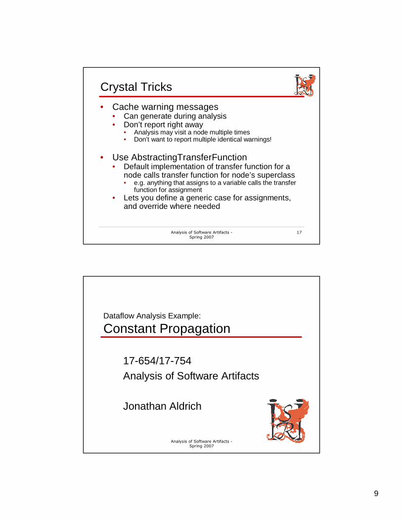
Crystal Tricks
• Cache warning messages• Can generate during analysis• Don’t report right away
• Analysis may visit a node multiple times• Don’t want to report multiple identical warnings!
• Use AbstractingTransferFunction• Default implementation of transfer function for a
node calls transfer function for node’s superclass• e.g. anything that assigns to a variable calls the transfer
function for assignment• Lets you define a generic case for assignments,
and override where needed
Analysis of Software Artifacts -Spring 2007
18
Dataflow Analysis Example:
Constant Propagation
17-654/17-754Analysis of Software Artifacts
Jonathan Aldrich
10
Analysis of Software Artifacts -Spring 2007
19
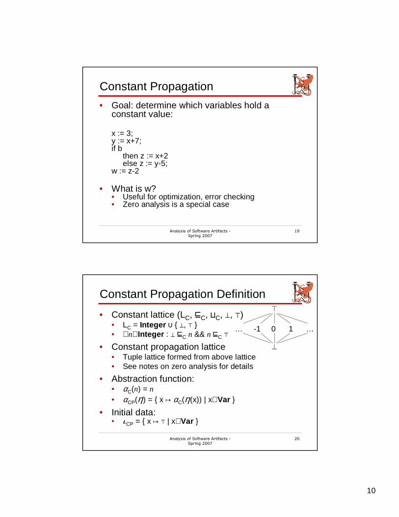
Constant Propagation
• Goal: determine which variables hold a constant value:
x := 3;y := x+7;if b
then z := x+2else z := y-5;
w := z-2
• What is w?• Useful for optimization, error checking• Zero analysis is a special case
Analysis of Software Artifacts -Spring 2007
20
Constant Propagation Definition
• Constant lattice (LC, ⊑C, ⊔C, ⊥, ⊤)• LC = Integer ⋃ { ⊥, ⊤ }• ∀n∈Integer : ⊥ ⊑C n && n ⊑C ⊤
• Constant propagation lattice• Tuple lattice formed from above lattice• See notes on zero analysis for details
• Abstraction function:• αC(n) = n• αCP(η) = { x ↦ αC(η(x)) | x∈Var }
• Initial data:• ιCP = { x ↦ ⊤ | x∈Var }
⊤
… -1 0 1 …
⊥
11
Analysis of Software Artifacts -Spring 2007
21
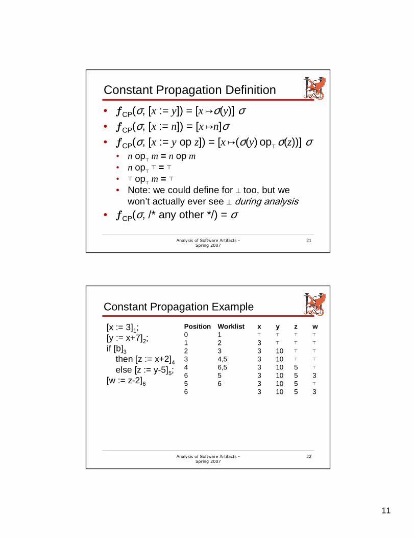
Constant Propagation Definition
• ƒCP(σ, [x := y]) = [x ↦σ(y)] σ• ƒCP(σ, [x := n]) = [x ↦n]σ• ƒCP(σ, [x := y op z]) = [x ↦(σ(y) op⊤ σ(z))] σ
• n op⊤ m = n op m• n op⊤ ⊤ = ⊤• ⊤ op⊤ m = ⊤• Note: we could define for ⊥ too, but we
won’t actually ever see ⊥ during analysis
• ƒCP(σ, /* any other */) = σ
Analysis of Software Artifacts -Spring 2007
22
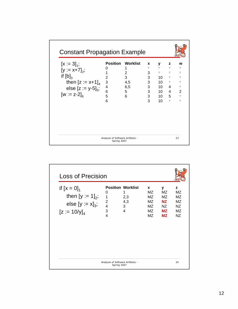
Constant Propagation Example
[x := 3]1;[y := x+7]2;if [b]3
then [z := x+2]4
else [z := y-5]5;[w := z-2]6
Position Worklist x y z w0 1 ⊤ ⊤ ⊤ ⊤
1 2 3 ⊤ ⊤ ⊤
2 3 3 10 ⊤ ⊤
3 4,5 3 10 ⊤ ⊤
4 6,5 3 10 5 ⊤
6 5 3 10 5 35 6 3 10 5 ⊤
6 3 10 5 3
12
Analysis of Software Artifacts -Spring 2007
23
Constant Propagation Example
[x := 3]1;[y := x+7]2;if [b]3
then [z := x+1]4
else [z := y-5]5;[w := z-2]6
Position Worklist x y z w0 1 ⊤ ⊤ ⊤ ⊤
1 2 3 ⊤ ⊤ ⊤
2 3 3 10 ⊤ ⊤
3 4,5 3 10 ⊤ ⊤
4 6,5 3 10 4 ⊤
6 5 3 10 4 25 6 3 10 5 ⊤
6 3 10 ⊤ ⊤
Analysis of Software Artifacts -Spring 2007
24
Loss of Precision
if [x = 0]1then [y := 1]2;
else [y := x]3;
[z := 10/y]4
Position Worklist x y z0 1 MZ MZ MZ1 2,3 MZ MZ MZ2 4,3 MZ NZ MZ4 3 MZ NZ NZ3 4 MZ MZ MZ4 MZ MZ NZ
13
Analysis of Software Artifacts -Spring 2007
25
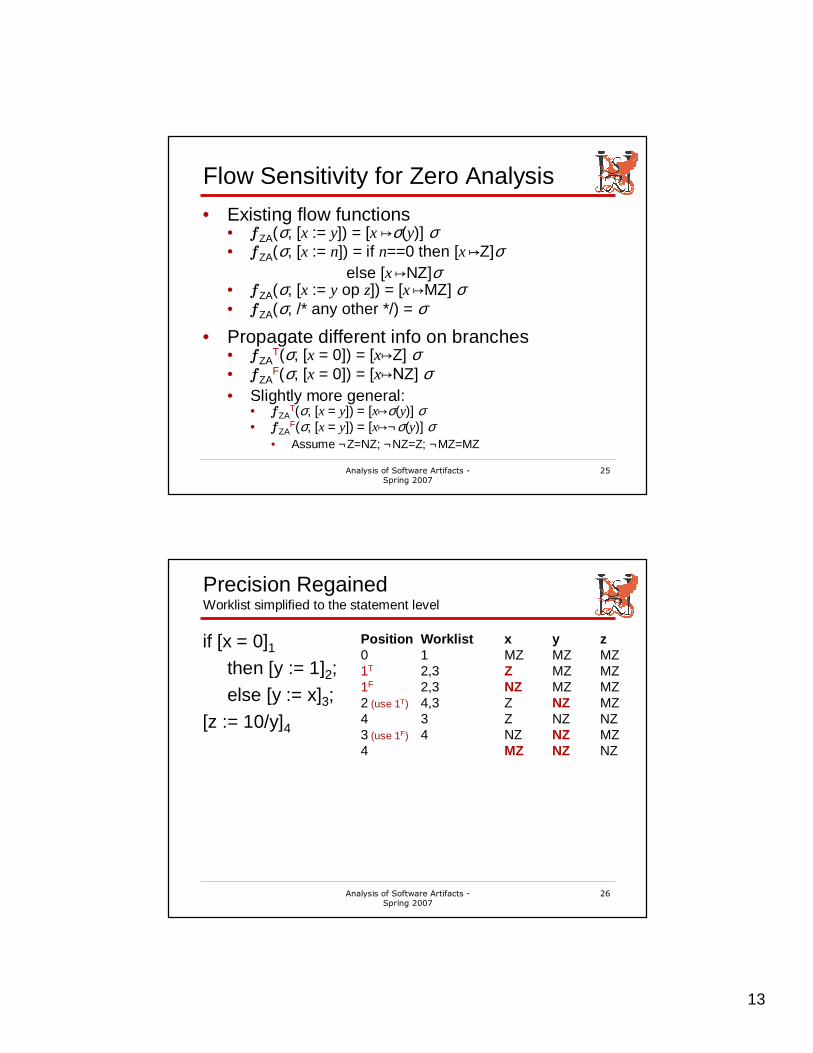
Flow Sensitivity for Zero Analysis
• Existing flow functions• ƒZA(σ, [x := y]) = [x ↦σ(y)] σ• ƒZA(σ, [x := n]) = if n==0 then [x ↦Z]σ
else [x ↦NZ]σ• ƒZA(σ, [x := y op z]) = [x ↦MZ] σ• ƒZA(σ, /* any other */) = σ
• Propagate different info on branches• ƒZA
T(σ, [x = 0]) = [x↦Z] σ• ƒZA
F(σ, [x = 0]) = [x↦NZ] σ• Slightly more general:
• ƒZAT(σ, [x = y]) = [x↦σ(y)] σ
• ƒZAF(σ, [x = y]) = [x↦¬σ(y)] σ
• Assume ¬Z=NZ; ¬NZ=Z; ¬MZ=MZ
Analysis of Software Artifacts -Spring 2007
26
Precision RegainedWorklist simplified to the statement level
if [x = 0]1then [y := 1]2;
else [y := x]3;
[z := 10/y]4
Position Worklist x y z0 1 MZ MZ MZ1T 2,3 Z MZ MZ1F 2,3 NZ MZ MZ2 (use 1T) 4,3 Z NZ MZ4 3 Z NZ NZ3 (use 1F) 4 NZ NZ MZ4 MZ NZ NZ
14
Analysis of Software Artifacts -Spring 2007
27
Dataflow Analysis Correctness
Software AnalysisLG Electronics Curriculum
Jonathan Aldrich
Analysis of Software Artifacts -Spring 2007
28
What does Correctness Mean?
• Intuition• Analysis will eventually terminate at a fixed
point• At a fixed point, analysis results are a sound
abstraction of program execution• program execution must be formally defined• abstraction function relates program
execution to data flow lattice elements• sound means truth ⊑ analysis results
• also called conservative or safe
15
Analysis of Software Artifacts -Spring 2007
29
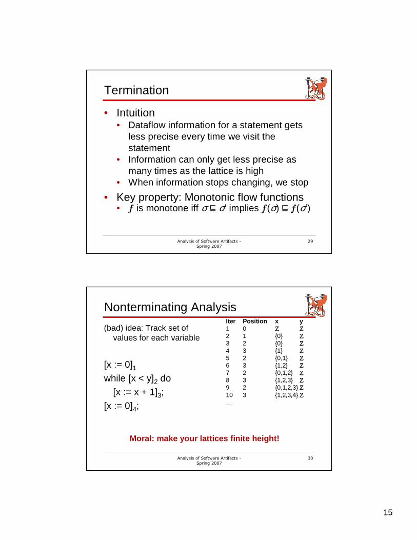
Termination
• Intuition• Dataflow information for a statement gets
less precise every time we visit the statement
• Information can only get less precise as many times as the lattice is high
• When information stops changing, we stop
• Key property: Monotonic flow functions• ƒ is monotone iff σ ⊑ σ′ implies ƒ(σ) ⊑ ƒ(σ′)
Analysis of Software Artifacts -Spring 2007
30
Nonterminating Analysis
(bad) idea: Track set of values for each variable
[x := 0]1while [x < y]2 do
[x := x + 1]3;
[x := 0]4;
Iter Position x y1 0 ℤℤℤℤ ℤℤℤℤ
2 1 {0} ℤℤℤℤ
3 2 {0} ℤℤℤℤ
4 3 {1} ℤℤℤℤ
5 2 {0,1} ℤℤℤℤ
6 3 {1,2} ℤℤℤℤ
7 2 {0,1,2} ℤℤℤℤ
8 3 {1,2,3} ℤℤℤℤ
9 2 {0,1,2,3} ℤℤℤℤ
10 3 {1,2,3,4} ℤℤℤℤ
…
Moral: make your lattices finite height!
16
Analysis of Software Artifacts -Spring 2007
31
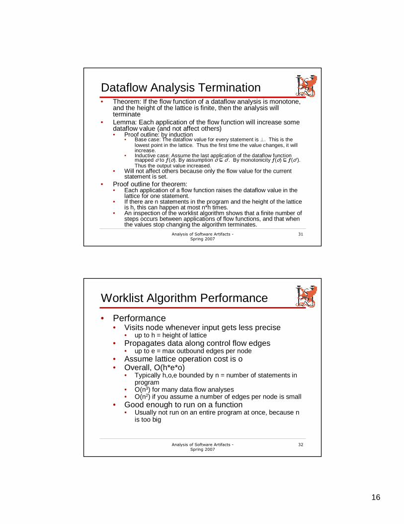
Dataflow Analysis Termination• Theorem: If the flow function of a dataflow analysis is monotone,
and the height of the lattice is finite, then the analysis will terminate
• Lemma: Each application of the flow function will increase some dataflow value (and not affect others)• Proof outline: by induction
• Base case: The dataflow value for every statement is ⊥. This is the lowest point in the lattice. Thus the first time the value changes, it will increase.
• Inductive case: Assume the last application of the dataflow function mapped σ to ƒ(σ). By assumption σ ⊑ σ′. By monotonicity ƒ(σ) ⊑ ƒ(σ′). Thus the output value increased.
• Will not affect others because only the flow value for the current statement is set.
• Proof outline for theorem:• Each application of a flow function raises the dataflow value in the
lattice for one statement.• If there are n statements in the program and the height of the lattice
is h, this can happen at most n*h times.• An inspection of the worklist algorithm shows that a finite number of
steps occurs between applications of flow functions, and that when the values stop changing the algorithm terminates.
Analysis of Software Artifacts -Spring 2007
32
Worklist Algorithm Performance
• Performance• Visits node whenever input gets less precise
• up to h = height of lattice• Propagates data along control flow edges
• up to e = max outbound edges per node• Assume lattice operation cost is o• Overall, O(h*e*o)
• Typically h,o,e bounded by n = number of statements in program
• O(n3) for many data flow analyses• O(n2) if you assume a number of edges per node is small
• Good enough to run on a function• Usually not run on an entire program at once, because n
is too big
17
Analysis of Software Artifacts -Spring 2007
33
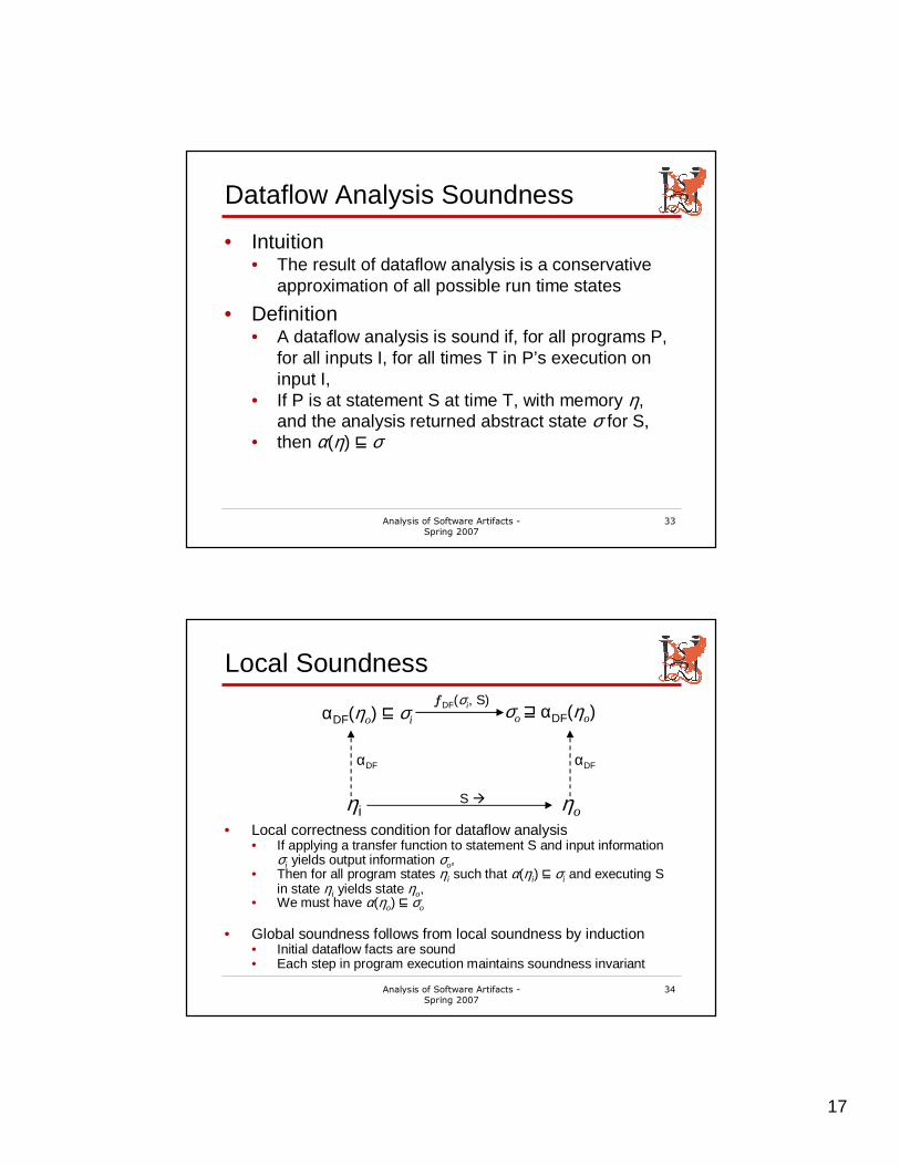
Dataflow Analysis Soundness
• Intuition• The result of dataflow analysis is a conservative
approximation of all possible run time states
• Definition• A dataflow analysis is sound if, for all programs P,
for all inputs I, for all times T in P’s execution on input I,
• If P is at statement S at time T, with memory η, and the analysis returned abstract state σ for S,
• then α(η) ⊑ σ
Analysis of Software Artifacts -Spring 2007
34
Local Soundness
• Local correctness condition for dataflow analysis• If applying a transfer function to statement S and input information
σi yields output information σo,• Then for all program states ηi such that α(ηi) ⊑ σi and executing S
in state ηi yields state ηo,• We must have α(ηo) ⊑ σo
• Global soundness follows from local soundness by induction• Initial dataflow facts are sound• Each step in program execution maintains soundness invariant
ηi ηo
αDF(ηo) ⊑ σi σo ⊒ αDF(ηo)ƒDF(σi, S)
S �
αDF αDF

18
Analysis of Software Artifacts -Spring 2007
35
Why care about Soundness?
• Analysis Producers• Writing analyses is hard
• People make mistakes all the time• Need to know how to think about correctness• When the analysis gets tricky, it’s useful to prove it correct
formally
• Analysis Consumers• Sound analysis provides guarantees
• Optimizations won’t break the program• Finds all defects of a certain sort
• Decision making• Knowledge of soundness techniques lets you ask the right
questions about a tool you are considering• Soundness affects where you invest QA resources
• Focus testing efforts on areas where you don’t have a sound analysis!
Analysis of Software Artifacts -Spring 2007
36
Additional Slides (for your reference)
19
Analysis of Software Artifacts -Spring 2007
37
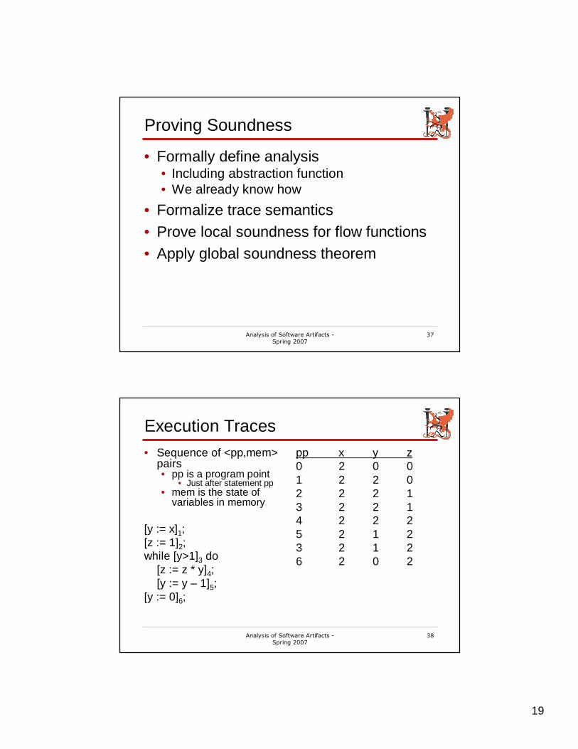
Proving Soundness
• Formally define analysis• Including abstraction function• We already know how
• Formalize trace semantics• Prove local soundness for flow functions• Apply global soundness theorem
Analysis of Software Artifacts -Spring 2007
38
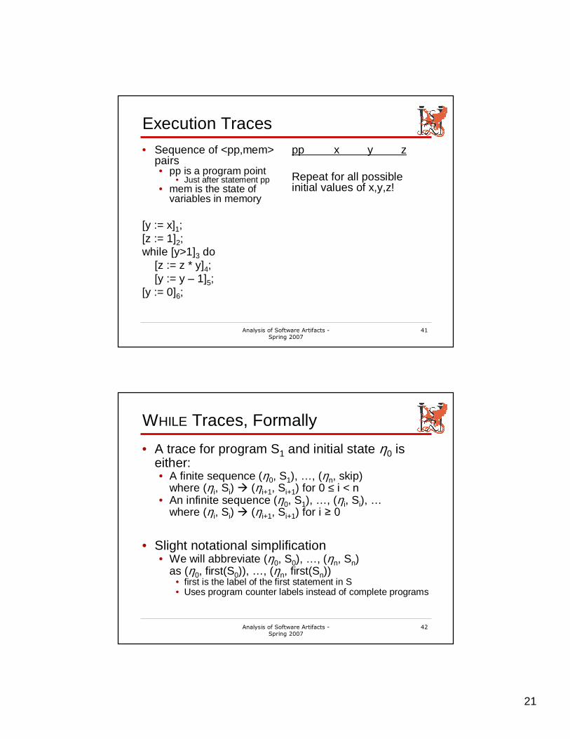
Execution Traces
• Sequence of <pp,mem> pairs• pp is a program point
• Just after statement pp• mem is the state of
variables in memory
[y := x]1;[z := 1]2;while [y>1]3 do
[z := z * y]4;[y := y – 1]5;
[y := 0]6;
pp x y z0 2 0 01 2 2 02 2 2 13 2 2 14 2 2 25 2 1 23 2 1 26 2 0 2
20
Analysis of Software Artifacts -Spring 2007
39
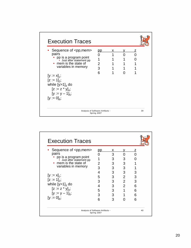
Execution Traces
• Sequence of <pp,mem> pairs• pp is a program point
• Just after statement pp• mem is the state of
variables in memory
[y := x]1;[z := 1]2;while [y>1]3 do
[z := z * y]4;[y := y – 1]5;
[y := 0]6;
pp x y z0 1 0 01 1 1 02 1 1 13 1 1 16 1 0 1
Analysis of Software Artifacts -Spring 2007
40
Execution Traces
• Sequence of <pp,mem> pairs• pp is a program point
• Just after statement pp• mem is the state of
variables in memory
[y := x]1;[z := 1]2;while [y>1]3 do
[z := z * y]4;[y := y – 1]5;
[y := 0]6;
pp x y z0 3 0 01 3 3 02 3 3 13 3 3 14 3 3 35 3 2 33 3 2 34 3 2 65 3 1 63 3 1 66 3 0 6
21
Analysis of Software Artifacts -Spring 2007
41
Execution Traces
• Sequence of <pp,mem> pairs• pp is a program point
• Just after statement pp• mem is the state of
variables in memory
[y := x]1;[z := 1]2;while [y>1]3 do
[z := z * y]4;[y := y – 1]5;
[y := 0]6;
pp x y z
Repeat for all possible initial values of x,y,z!
Analysis of Software Artifacts -Spring 2007
42
WHILE Traces, Formally
• A trace for program S1 and initial state η0 is either:• A finite sequence (η0, S1), …, (ηn, skip)
where (ηi, Si) � (ηi+1, Si+1) for 0 ≤ i < n• An infinite sequence (η0, S1), …, (ηi, Si), …
where (ηi, Si) � (ηi+1, Si+1) for i ≥ 0
• Slight notational simplification• We will abbreviate (η0, S0), …, (ηn, Sn)
as (η0, first(S0)), …, (ηn, first(Sn))• first is the label of the first statement in S• Uses program counter labels instead of complete programs
22
Analysis of Software Artifacts -Spring 2007
43
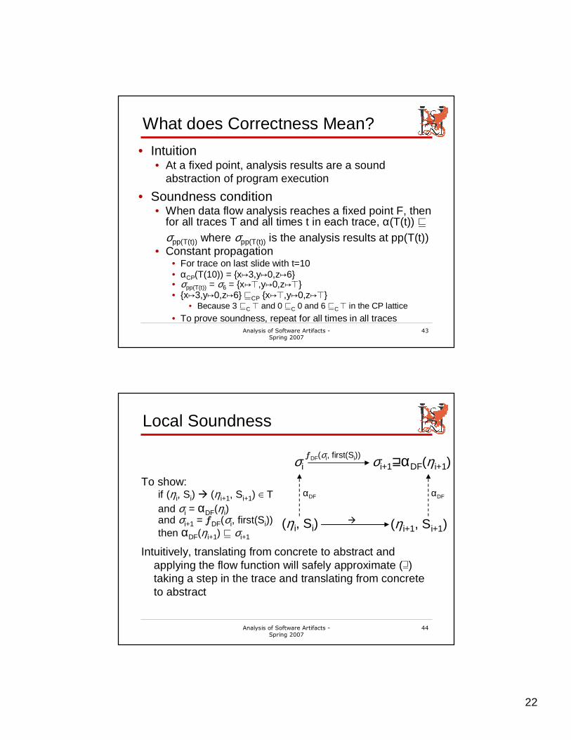
What does Correctness Mean?
• Intuition• At a fixed point, analysis results are a sound
abstraction of program execution
• Soundness condition• When data flow analysis reaches a fixed point F, then
for all traces T and all times t in each trace, α(T(t)) ⊑σpp(T(t)) where σpp(T(t)) is the analysis results at pp(T(t))
• Constant propagation• For trace on last slide with t=10• αCP(T(10)) = {x↦3,y↦0,z↦6}• σpp(T(t)) = σ6 = {x↦⊤,y↦0,z↦⊤}• {x↦3,y↦0,z↦6} ⊑CP {x↦⊤,y↦0,z↦⊤}
• Because 3 ⊑C ⊤ and 0 ⊑C 0 and 6 ⊑C ⊤ in the CP lattice
• To prove soundness, repeat for all times in all traces
Analysis of Software Artifacts -Spring 2007
44
Local Soundness
To show:if (ηi, Si) � (ηi+1, Si+1) ∈ Tand σi = αDF(ηi)and σi+1 = ƒDF(σi, first(Si))then αDF(ηi+1) ⊑ σi+1
Intuitively, translating from concrete to abstract and applying the flow function will safely approximate (⊒) taking a step in the trace and translating from concrete to abstract
(ηi, Si) (ηi+1, Si+1)
σi σi+1⊒αDF(ηi+1)ƒDF(σi, first(Si))
�
αDF αDF
23
Analysis of Software Artifacts -Spring 2007
45
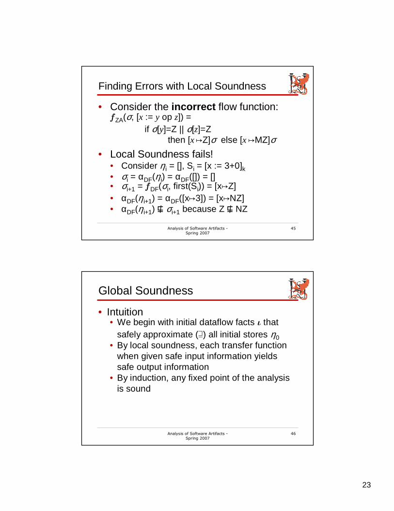
Finding Errors with Local Soundness
• Consider the incorrect flow function:ƒZA(σ, [x := y op z]) =
if σ[y]=Z || σ[z]=Zthen [x ↦Z]σ else [x ↦MZ]σ
• Local Soundness fails!• Consider ηi = [], Si = [x := 3+0]k• σi = αDF(ηi) = αDF([]) = []• σi+1 = ƒDF(σi, first(Si)) = [x↦Z]• αDF(ηi+1) = αDF([x↦3]) = [x↦NZ]• αDF(ηi+1) ⋢ σi+1 because Z ⋢ NZ
Analysis of Software Artifacts -Spring 2007
46
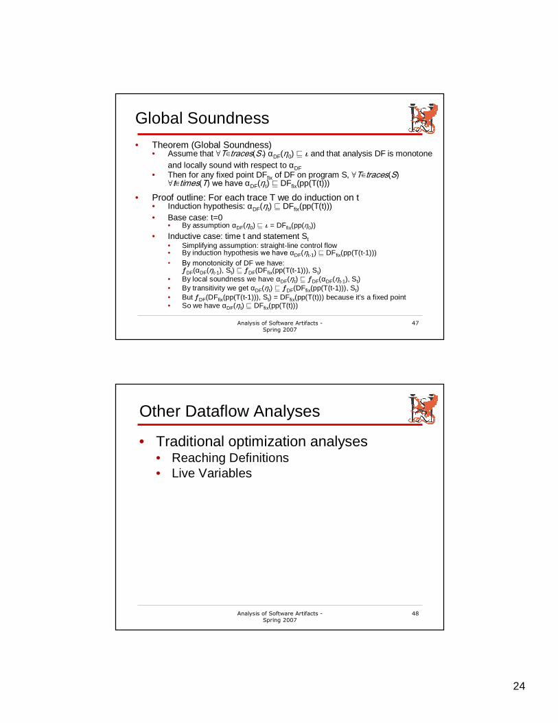
Global Soundness
• Intuition• We begin with initial dataflow facts ι that
safely approximate (⊒) all initial stores η0• By local soundness, each transfer function
when given safe input information yields safe output information
• By induction, any fixed point of the analysis is sound
24
Analysis of Software Artifacts -Spring 2007
47
Global Soundness
• Theorem (Global Soundness)• Assume that ∀T∈traces(S*) αDF(η0) ⊑ ι and that analysis DF is monotone
and locally sound with respect to αDF• Then for any fixed point DFfix of DF on program S, ∀T∈traces(S)
∀t∈times(T) we have αDF(ηt) ⊑ DFfix(pp(T(t)))
• Proof outline: For each trace T we do induction on t• Induction hypothesis: αDF(ηt) ⊑ DFfix(pp(T(t)))• Base case: t=0
• By assumption αDF(η0) ⊑ ι = DFfix(pp(η0))
• Inductive case: time t and statement St• Simplifying assumption: straight-line control flow• By induction hypothesis we have αDF(ηt-1) ⊑ DFfix(pp(T(t-1)))• By monotonicity of DF we have: ƒDF(αDF(ηt-1), St) ⊑ ƒDF(DFfix(pp(T(t-1))), St)
• By local soundness we have αDF(ηt) ⊑ ƒDF(αDF(ηt-1), St)• By transitivity we get αDF(ηt) ⊑ ƒDF(DFfix(pp(T(t-1))), St)• But ƒDF(DFfix(pp(T(t-1))), St) = DFfix(pp(T(t))) because it’s a fixed point• So we have αDF(ηt) ⊑ DFfix(pp(T(t)))
Analysis of Software Artifacts -Spring 2007
48
Other Dataflow Analyses
• Traditional optimization analyses• Reaching Definitions• Live Variables
25
Analysis of Software Artifacts -Spring 2007
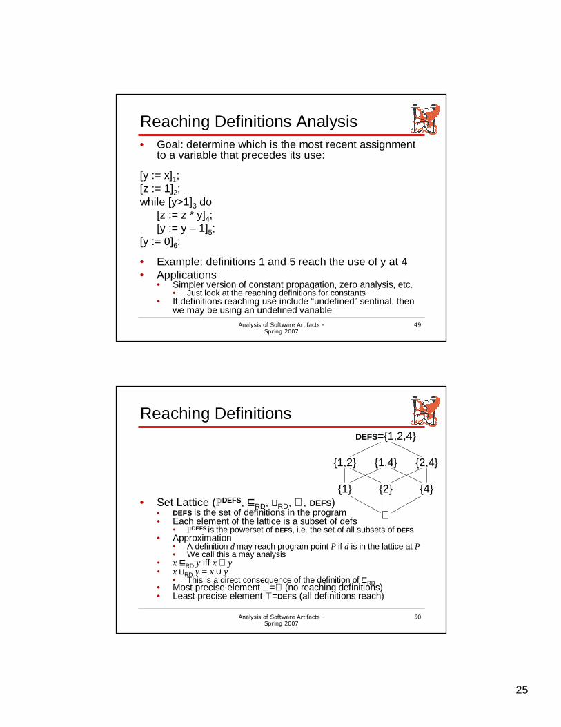
49
Reaching Definitions Analysis• Goal: determine which is the most recent assignment
to a variable that precedes its use:
[y := x]1;[z := 1]2;while [y>1]3 do
[z := z * y]4;[y := y – 1]5;
[y := 0]6;
• Example: definitions 1 and 5 reach the use of y at 4• Applications
• Simpler version of constant propagation, zero analysis, etc.• Just look at the reaching definitions for constants
• If definitions reaching use include “undefined” sentinal, then we may be using an undefined variable
Analysis of Software Artifacts -Spring 2007
50
Reaching Definitions
• Set Lattice (ℙDEFS, ⊑RD, ⊔RD, ∅, DEFS)• DEFS is the set of definitions in the program• Each element of the lattice is a subset of defs
• ℙDEFS is the powerset of DEFS, i.e. the set of all subsets of DEFS• Approximation
• A definition d may reach program point P if d is in the lattice at P• We call this a may analysis
• x ⊑RD y iff x ⊆ y• x ⊔RD y = x ⋃ y
• This is a direct consequence of the definition of ⊑RD• Most precise element ⊥=∅ (no reaching definitions)• Least precise element ⊤=DEFS (all definitions reach)
DEFS={1,2,4}
{1,2} {1,4} {2,4}
{1} {2} {4}
∅
26
Analysis of Software Artifacts -Spring 2007
51
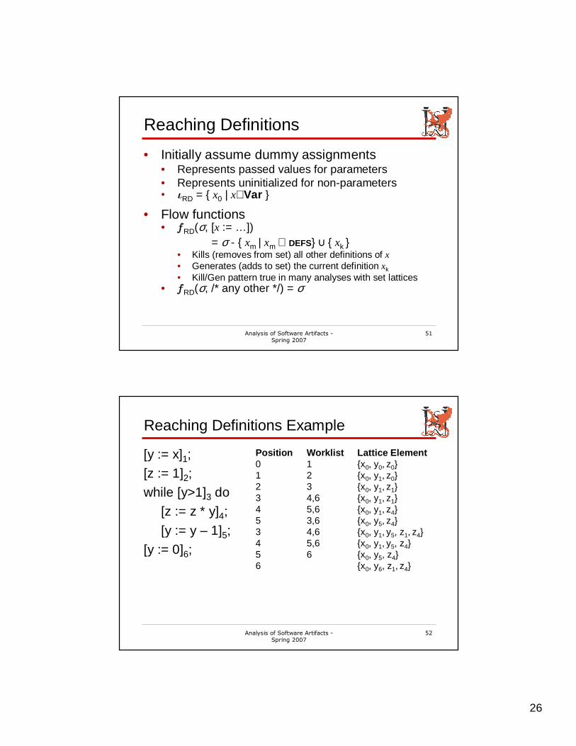
Reaching Definitions
• Initially assume dummy assignments• Represents passed values for parameters• Represents uninitialized for non-parameters• ιRD = { x0 | x∈Var }
• Flow functions• ƒRD(σ, [x := …])
= σ - { xm | xm ∈ DEFS} ⋃ { xk }• Kills (removes from set) all other definitions of x• Generates (adds to set) the current definition xk
• Kill/Gen pattern true in many analyses with set lattices• ƒRD(σ, /* any other */) = σ
Analysis of Software Artifacts -Spring 2007
52
Reaching Definitions Example
[y := x]1;
[z := 1]2;
while [y>1]3 do
[z := z * y]4;
[y := y – 1]5;
[y := 0]6;
Position Worklist Lattice Element0 1 {x0, y0, z0}1 2 {x0, y1, z0}2 3 {x0, y1, z1}3 4,6 {x0, y1, z1}4 5,6 {x0, y1, z4}5 3,6 {x0, y5, z4}3 4,6 {x0, y1, y5, z1, z4}4 5,6 {x0, y1, y5, z4}5 6 {x0, y5, z4}6 {x0, y6, z1, z4}
27
Analysis of Software Artifacts -Spring 2007
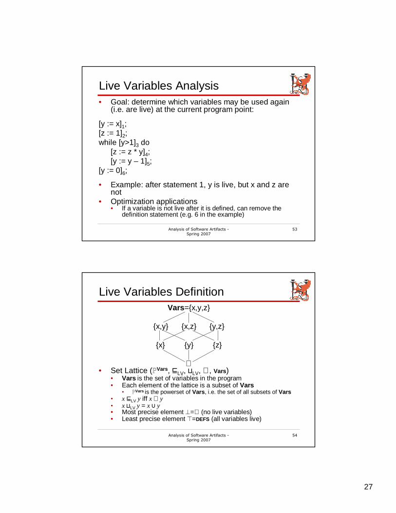
53
Live Variables Analysis• Goal: determine which variables may be used again
(i.e. are live) at the current program point:
[y := x]1;[z := 1]2;while [y>1]3 do
[z := z * y]4;[y := y – 1]5;
[y := 0]6;
• Example: after statement 1, y is live, but x and z are not
• Optimization applications• If a variable is not live after it is defined, can remove the
definition statement (e.g. 6 in the example)
Analysis of Software Artifacts -Spring 2007
54
Live Variables Definition
• Set Lattice (ℙVars, ⊑LV, ⊔LV, ∅, Vars)• Vars is the set of variables in the program• Each element of the lattice is a subset of Vars
• ℙVars is the powerset of Vars, i.e. the set of all subsets of Vars• x ⊑LV y iff x ⊆ y• x ⊔LV y = x ⋃ y• Most precise element ⊥=∅ (no live variables)• Least precise element ⊤=DEFS (all variables live)
Vars={x,y,z}
{x,y} {x,z} {y,z}
{x} {y} {z}
∅
28
Analysis of Software Artifacts -Spring 2007
55
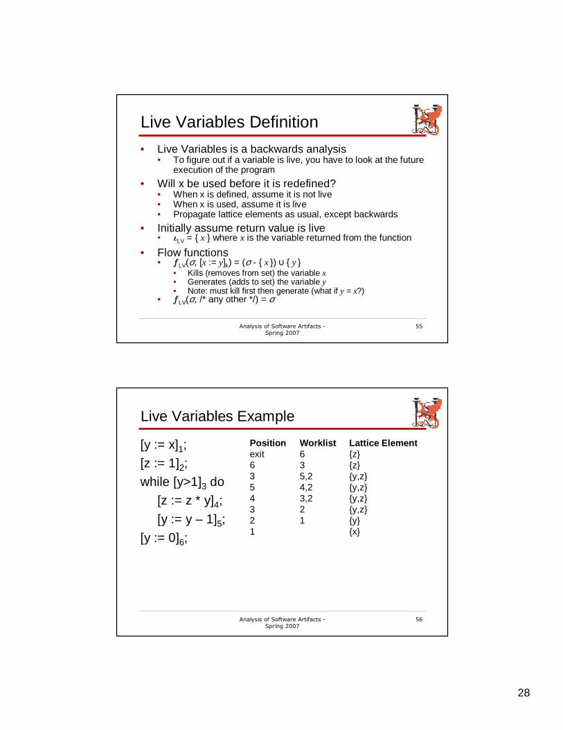
Live Variables Definition
• Live Variables is a backwards analysis• To figure out if a variable is live, you have to look at the future
execution of the program
• Will x be used before it is redefined?• When x is defined, assume it is not live• When x is used, assume it is live• Propagate lattice elements as usual, except backwards
• Initially assume return value is live• ιLV = { x } where x is the variable returned from the function
• Flow functions• ƒLV(σ, [x := y]k) = (σ - { x }) ⋃ { y }
• Kills (removes from set) the variable x• Generates (adds to set) the variable y• Note: must kill first then generate (what if y = x?)
• ƒLV(σ, /* any other */) = σ
Analysis of Software Artifacts -Spring 2007
56
Live Variables Example
[y := x]1;
[z := 1]2;
while [y>1]3 do
[z := z * y]4;
[y := y – 1]5;
[y := 0]6;
Position Worklist Lattice Elementexit 6 {z}6 3 {z}3 5,2 {y,z}5 4,2 {y,z}4 3,2 {y,z}3 2 {y,z}2 1 {y}1 {x}