Data Compression - Τμήμα Επιστήμης Υπολογιστών...

Data CompressionKhalid SayoodUniversity of Nebraska, Lincoln

Encyclopedia of Information Systems, Volume 1Copyright 2003, Elsevier Science (USA). All rights reserved. 423

I. INTRODUCTIONII. LOSSLESS COMPRESSION

III. LOSSY COMPRESSIONIV. FURTHER INFORMATION

I. INTRODUCTION

Data compression involves the development of a com-pact representation of information. Most representa-tions of information contain large amounts of redun-dancy. Redundancy can exist in various forms. It mayexist in the form of correlation: spatially close pixels inan image are generally also close in value. The redun-dancy might be due to context: the number of possi-bilities for a particular letter in a piece of English textis drastically reduced if the previous letter is a q. It canbe probabilistic in nature: the letter e is much morelikely to occur in a piece of English text than the letterq. It can be a result of how the information-bearing se-quence was generated: voiced speech has a periodicstructure. Or, the redundancy can be a function of theuser of the information: when looking at an image wecannot see above a certain spatial frequency; therefore,the high-frequency information is redundant for thisapplication. Redundancy is defined by the Merriam-Webster Dictionary as “the part of the message that canbe eliminated without the loss of essential informa-tion.” Therefore, one aspect of data compression is re-dundancy removal. Characterization of redundancy in-volves some form of modeling. Hence, this step in thecompression process is also known as modeling. Forhistorical reasons another name applied to this processis decorrelation.

After the redundancy removal process the infor-mation needs to be encoded into a binary represen-tation. At this stage we make use of the fact that if theinformation is represented using a particular alpha-bet some letters may occur with higher probabilitythan others. In the coding step we use shorter code

words to represent letters that occur more frequently,thus lowering the average number of bits required torepresent each letter.

Compression in all its forms exploits structure, orredundancy, in the data to achieve a compact repre-sentation. The design of a compression algorithm in-volves understanding the types of redundancy presentin the data and then developing strategies for ex-ploiting these redundancies to obtain a compact rep-resentation of the data. People have come up withmany ingenious ways of characterizing and using thedifferent types of redundancies present in differentkinds of technologies from the telegraph to the cellular phone and digital movies.

One way of classifying compression schemes is bythe model used to characterize the redundancy. How-ever, more popularly, compression schemes are di-vided into two main groups: lossless compression andlossy compression. Lossless compression preserves allthe information in the data being compressed, andthe reconstruction is identical to the original data. Inlossy compression some of the information containedin the original data is irretrievably lost. The loss in in-formation is, in some sense, a payment for achievinghigher levels of compression. We begin our examina-tion of data compression schemes by first looking atlossless compression techniques.

II. LOSSLESS COMPRESSION

Lossless compression involves finding a representationwhich will exactly represent the source. There shouldbe no loss of information, and the decompressed, or

reconstructed, sequence should be identical to theoriginal sequence. The requirement that there be noloss of information puts a limit on how much com-pression we can get. We can get some idea about thislimit by looking at some concepts from informationtheory.

A. Information and Entropy

In one sense it is impossible to denote anyone as theparent of data compression: people have been findingcompact ways of representing information since thedawn of recorded history. One could argue that thedrawings on the cave walls are representations of a sig-nificant amount of information and therefore qualify asa form of data compression. Significantly less contro-versial would be the characterizing of the Morse codeas a form of data compression. Samuel Morse took ad-vantage of the fact that certain letters such as e and aoccur more frequently in the English language than qor z to assign shorter code words to the more frequentlyoccurring letters. This results in lower average trans-mission time per letter. The first person to put datacompression on a sound theoretical footing was ClaudeE. Shannon (1948). He developed a quantitative notionof information that formed the basis of a mathematicalrepresentation of the communication process.

Suppose we conduct a series of independent ex-periments where each experiment has outcomes A1,A2, . . ., AM. Shannon associated with each outcome aquantity called self information, defined as

i(Ak) � log �P(

1Ak)�

The units of self-information are bits, nats, or Hart-leys, depending on whether the base of the logarithm

is 2 e, or 10. The average amount of information as-sociated with the experiment is called the entropy H:

H � E[i(A)] � �M

k�1i(Ak)P(Ak) � �

M

k�1P(Ak) log �

P(1Ak)�

� � �M

k�1P(Ak) log P(Ak) (1)

Suppose the “experiment” is the generation of a let-ter by a source, and further suppose the source gen-erates each letter independently according to someprobability model. Then H as defined in Eq. (1) iscalled the entropy of the source. Shannon showedthat if we compute the entropy in bits (use logarithmbase 2) the entropy is the smallest average number ofbits needed to represent the source output.

We can get an intuitive feel for this connection be-tween the entropy of a source and the average num-ber of bits needed to represent its output (denoted byrate) by performing a couple of experiments.

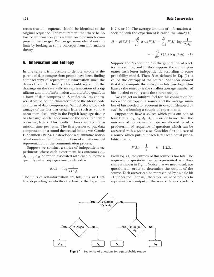
Suppose we have a source which puts out one offour letters {A1, A2, A3, A4}. In order to ascertain theoutcome of the experiment we are allowed to ask apredetermined sequence of questions which can beanswered with a yes or a no. Consider first the case ofa source which puts out each letter with equal proba-bility, that is,

P(Ak) � �14

� k � 1,2,3,4

From Eq. (1) the entropy of this source is two bits. Thesequence of questions can be represented as a flow-chart as shown in Fig. 1. Notice that we need to ask twoquestions in order to determine the output of thesource. Each answer can be represented by a single bit(1 for yes and 0 for no); therefore, we need two bits torepresent each output of the source. Now consider a

424 Data Compression

Figure 1 Sequence of questions for equiprobable source.

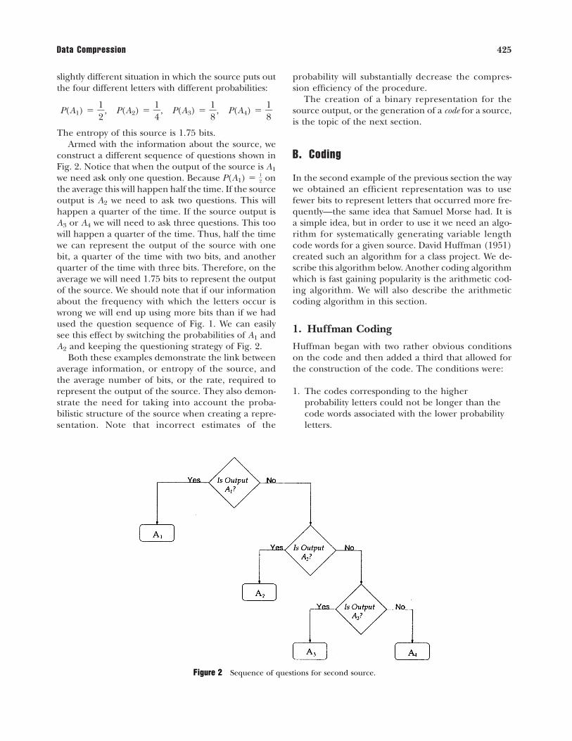
slightly different situation in which the source puts outthe four different letters with different probabilities:

P(A1) � �12

�, P(A2) � �14

�, P(A3) � �18

�, P(A4) � �18

�

The entropy of this source is 1.75 bits.Armed with the information about the source, we

construct a different sequence of questions shown inFig. 2. Notice that when the output of the source is A1

we need ask only one question. Because P(A1) � �12

� onthe average this will happen half the time. If the sourceoutput is A2 we need to ask two questions. This willhappen a quarter of the time. If the source output isA3 or A4 we will need to ask three questions. This toowill happen a quarter of the time. Thus, half the timewe can represent the output of the source with onebit, a quarter of the time with two bits, and anotherquarter of the time with three bits. Therefore, on theaverage we will need 1.75 bits to represent the outputof the source. We should note that if our informationabout the frequency with which the letters occur iswrong we will end up using more bits than if we hadused the question sequence of Fig. 1. We can easilysee this effect by switching the probabilities of A1 andA2 and keeping the questioning strategy of Fig. 2.

Both these examples demonstrate the link betweenaverage information, or entropy of the source, andthe average number of bits, or the rate, required torepresent the output of the source. They also demon-strate the need for taking into account the proba-bilistic structure of the source when creating a repre-sentation. Note that incorrect estimates of the

probability will substantially decrease the compres-sion efficiency of the procedure.

The creation of a binary representation for thesource output, or the generation of a code for a source,is the topic of the next section.

B. Coding

In the second example of the previous section the waywe obtained an efficient representation was to usefewer bits to represent letters that occurred more fre-quently—the same idea that Samuel Morse had. It isa simple idea, but in order to use it we need an algo-rithm for systematically generating variable lengthcode words for a given source. David Huffman (1951)created such an algorithm for a class project. We de-scribe this algorithm below. Another coding algorithmwhich is fast gaining popularity is the arithmetic cod-ing algorithm. We will also describe the arithmeticcoding algorithm in this section.

1. Huffman Coding

Huffman began with two rather obvious conditionson the code and then added a third that allowed forthe construction of the code. The conditions were:

1. The codes corresponding to the higherprobability letters could not be longer than thecode words associated with the lower probabilityletters.

Data Compression 425

Figure 2 Sequence of questions for second source.

2. The two lowest probability letters had to havecode words of the same length.

He added a third condition to generate a practicalcompression scheme.

3. The two lowest probability letters have codes thatare identical except for the last bit.

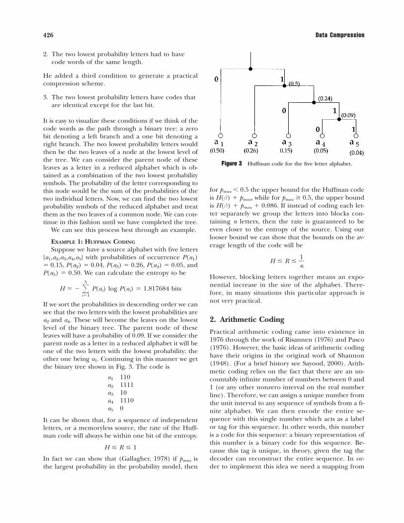
It is easy to visualize these conditions if we think of thecode words as the path through a binary tree: a zerobit denoting a left branch and a one bit denoting aright branch. The two lowest probability letters wouldthen be the two leaves of a node at the lowest level ofthe tree. We can consider the parent node of theseleaves as a letter in a reduced alphabet which is ob-tained as a combination of the two lowest probabilitysymbols. The probability of the letter corresponding tothis node would be the sum of the probabilities of thetwo individual letters. Now, we can find the two lowestprobability symbols of the reduced alphabet and treatthem as the two leaves of a common node. We can con-tinue in this fashion until we have completed the tree.

We can see this process best through an example.

EXAMPLE 1: HUFFMAN CODING

Suppose we have a source alphabet with five letters{a1,a2,a3,a4,a5} with probabilities of occurrence P(a1)� 0.15, P(a2) � 0.04, P(a3) � 0.26, P(a4) � 0.05, andP(a5) � 0.50. We can calculate the entropy to be

H � � �5

i�1P(ai) log P(ai) � 1.817684 bits

If we sort the probabilities in descending order we cansee that the two letters with the lowest probabilities area2 and a4. These will become the leaves on the lowestlevel of the binary tree. The parent node of theseleaves will have a probability of 0.09. If we consider theparent node as a letter in a reduced alphabet it will beone of the two letters with the lowest probability: theother one being a1. Continuing in this manner we getthe binary tree shown in Fig. 3. The code is

a1 110a2 1111a3 10a4 1110a5 0

It can be shown that, for a sequence of independentletters, or a memoryless source, the rate of the Huff-man code will always be within one bit of the entropy.

H � R � 1

In fact we can show that (Gallagher, 1978) if pmax isthe largest probability in the probability model, then

for pmax � 0.5 the upper bound for the Huffman codeis H(S) � pmax, while for pmax � 0.5, the upper boundis H(S) � pmax � 0.086. If instead of coding each let-ter separately we group the letters into blocks con-taining n letters, then the rate is guaranteed to beeven closer to the entropy of the source. Using ourlooser bound we can show that the bounds on the av-erage length of the code will be

H � R � �n1

�

However, blocking letters together means an expo-nential increase in the size of the alphabet. There-fore, in many situations this particular approach isnot very practical.

2. Arithmetic Coding

Practical arithmetic coding came into existence in1976 through the work of Risannen (1976) and Pasco(1976). However, the basic ideas of arithmetic codinghave their origins in the original work of Shannon(1948). (For a brief history see Sayood, 2000). Arith-metic coding relies on the fact that there are an un-countably infinite number of numbers between 0 and1 (or any other nonzero interval on the real numberline). Therefore, we can assign a unique number fromthe unit interval to any sequence of symbols from a fi-nite alphabet. We can then encode the entire se-quence with this single number which acts as a labelor tag for this sequence. In other words, this numberis a code for this sequence: a binary representation ofthis number is a binary code for this sequence. Be-cause this tag is unique, in theory, given the tag thedecoder can reconstruct the entire sequence. In or-der to implement this idea we need a mapping from


Figure 3 Huffman code for the five letter alphabet.

the sequence to the tag and an inverse mapping fromthe tag to the sequence.

One particular mapping is the cumulative densityfunction of the sequence. Let us view the sequence tobe encoded as the realization of a sequence of ran-dom variables {X1, X2, } and represent the set of allpossible realizations which have nonzero probabilityof occurrence in lexicographic order by {Xi}. Given aparticular realization

Xk � xk,1,xk,2,

the cumulative distribution function FX(xk,1,xk,2, ) isa number between 0 and 1. Furthermore, as we areonly dealing with sequences with nonzero probability,this number is unique to the sequence Xk. In fact, wecan uniquely assign the half-open interval [FX(Xk�1),FX(Xk�1)) to the sequence Xk. Any number in this in-terval, which we will refer to as the tag interval for Xk,can be used as a label or tag for the sequence Xk. Thearithmetic coding algorithm is essentially the calcula-tion of the end points of this tag interval. Before wedescribe the algorithm for computing these endpoints let us look at an example for a sequence ofmanageable length.

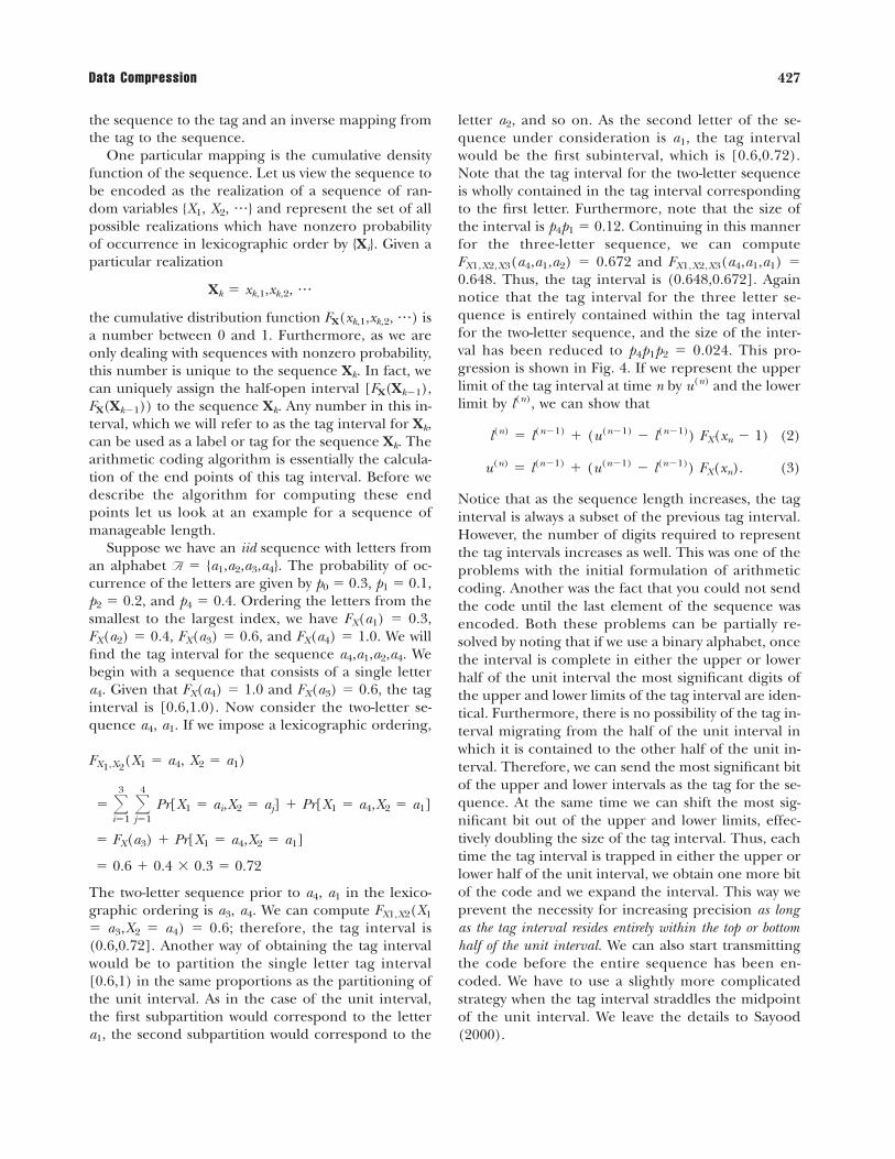
Suppose we have an iid sequence with letters froman alphabet A � {a1,a2,a3,a4}. The probability of oc-currence of the letters are given by p0 � 0.3, p1 � 0.1,p2 � 0.2, and p4 � 0.4. Ordering the letters from thesmallest to the largest index, we have FX(a1) � 0.3,FX(a2) � 0.4, FX(a3) � 0.6, and FX(a4) � 1.0. We willfind the tag interval for the sequence a4,a1,a2,a4. Webegin with a sequence that consists of a single lettera4. Given that FX(a4) � 1.0 and FX(a3) � 0.6, the taginterval is [0.6,1.0). Now consider the two-letter se-quence a4, a1. If we impose a lexicographic ordering,

FX1,X2(X1 � a4, X2 � a1)

� �3

i�1�4

j�1Pr[X1 � ai,X2 � aj] � Pr[X1 � a4,X2 � a1]

� FX(a3) � Pr[X1 � a4,X2 � a1]

� 0.6 � 0.4 0.3 � 0.72

The two-letter sequence prior to a4, a1 in the lexico-graphic ordering is a3, a4. We can compute FX1,X2(X1

� a3,X2 � a4) � 0.6; therefore, the tag interval is(0.6,0.72]. Another way of obtaining the tag intervalwould be to partition the single letter tag interval[0.6,1) in the same proportions as the partitioning ofthe unit interval. As in the case of the unit interval,the first subpartition would correspond to the lettera1, the second subpartition would correspond to the

letter a2, and so on. As the second letter of the se-quence under consideration is a1, the tag intervalwould be the first subinterval, which is [0.6,0.72).Note that the tag interval for the two-letter sequenceis wholly contained in the tag interval correspondingto the first letter. Furthermore, note that the size ofthe interval is p4p1 � 0.12. Continuing in this mannerfor the three-letter sequence, we can computeFX1,X2,X3(a4,a1,a2) � 0.672 and FX1,X2,X3(a4,a1,a1) �0.648. Thus, the tag interval is (0.648,0.672]. Againnotice that the tag interval for the three letter se-quence is entirely contained within the tag intervalfor the two-letter sequence, and the size of the inter-val has been reduced to p4p1p2 � 0.024. This pro-gression is shown in Fig. 4. If we represent the upperlimit of the tag interval at time n by u(n) and the lowerlimit by l(n), we can show that

l(n) � l(n�1) � (u(n�1) � l(n�1)) FX(xn � 1) (2)

u(n) � l(n�1) � (u(n�1) � l(n�1)) FX(xn). (3)

Notice that as the sequence length increases, the taginterval is always a subset of the previous tag interval.However, the number of digits required to representthe tag intervals increases as well. This was one of theproblems with the initial formulation of arithmeticcoding. Another was the fact that you could not sendthe code until the last element of the sequence wasencoded. Both these problems can be partially re-solved by noting that if we use a binary alphabet, oncethe interval is complete in either the upper or lowerhalf of the unit interval the most significant digits ofthe upper and lower limits of the tag interval are iden-tical. Furthermore, there is no possibility of the tag in-terval migrating from the half of the unit interval inwhich it is contained to the other half of the unit in-terval. Therefore, we can send the most significant bitof the upper and lower intervals as the tag for the se-quence. At the same time we can shift the most sig-nificant bit out of the upper and lower limits, effec-tively doubling the size of the tag interval. Thus, eachtime the tag interval is trapped in either the upper orlower half of the unit interval, we obtain one more bitof the code and we expand the interval. This way weprevent the necessity for increasing precision as longas the tag interval resides entirely within the top or bottomhalf of the unit interval. We can also start transmittingthe code before the entire sequence has been en-coded. We have to use a slightly more complicatedstrategy when the tag interval straddles the midpointof the unit interval. We leave the details to Sayood(2000).


C. Sources with Memory

Throughout our discussion we have been assumingthat each symbol in a sequence occurs independentlyof the previous sequence. In other words, there is nomemory in the sequence. Most sequences of interest tous are not made up of independently occurring sym-bols. In such cases an assumption of independencewould give us an incorrect estimate of the probabilityof occurrence of that symbol, thus leading to an inef-ficient code. By taking account of the dependenciesin the sequence we can significantly improve theamount of compression available. Consider the letteru in a piece of English text. The frequency of occur-rence of the letter u occurring in a piece of Englishtext is approximately 0.018. If we had to encode theletter u and we used this value as our estimate of theprobability of the letter, we would need approximatelylog2 �

0.0118� � 6 bits. However, if we knew the previous

letter was q our estimate of the probability of the let-ter u would be substantially more than 0.018 and thusencoding u would require fewer bits. Another way oflooking at this is by noting that if we have an accurateestimate of the probability of occurrence of particularsymbols we can obtain a much more efficient code. Ifwe know the preceding letter(s) we can obtain a moreaccurate estimate of the probabilities of occurrenceof the letters that follow. Similarly, if we look at pixelvalues in a natural image and assume that the pixelsoccur independently, then our estimate of the proba-bility of the values that each pixel could take on wouldbe approximately the same (and small). If we tookinto account the values of the neighboring pixels, the

probability that the pixel under consideration wouldhave a similar value would be quite high. If, in fact,the pixel had a value close to its neighbors, encodingit in this context would require many fewer bits thanencoding it independent of its neighbors (Memonand Sayood, 1995).

Shannon (1948) incorporated this dependence in the definition of entropy in the following manner.Define

Gn � � �i1�m

i1�m �

i2�m

i2�m �

in�m

in�1

P(X1 � i1,X2 � i2, . . ., Xn � in)

log P(X1 � i1,X2 � i2,. . . ,Xn � in)

where {X1,X2, . . .,Xn} is a sequence of length n gen-erated by a source S. Then the entropy of the sourceis defined as

H(S) � limn→�

�n1

� Gn

There are a large number of compression schemesthat make use of this dependence.

D. Context-Based Coding

The most direct approach to using this dependenceis to code each symbol based on the probabilities pro-vided by the context. If we are to sequentially encodethe sequence x1,x2, . . .,xn, we need � log �i�0

n�1

p(xi�1|x1,x2, . . .,xn) bits (Weinberger et al., 1995). Thehistory of the sequence makes up its context. In prac-


0.648

0.6552

0.6576

0.6624

0.67200.720

0.672

0.648

0.636

0.600

0.84

0.76

0.72

0.6

1.0

a4

a3

a2

a1

0.3

0.0

0.4

0.6

1.0

Figure 4 Narrowing of the tag interval for the sequence a4a0a2a4.

tice, if we had these probabilities available they couldbe used by an arithmetic coder to code the particularsymbol. To use the entire history of the sequence asthe context is generally not feasible. Therefore, thecontext is made up of some subset of the history. Itgenerally consists of those symbols that our knowl-edge of the source tells us will have an affect on theprobability of the symbol being encoded and whichare available to both the encoder and the decoder.For example, in the binary image coding standardJBIG, the context may consist of the pixels in the im-mediate neighborhood of the pixel being encodedalong with a pixel some distance away which reflectsthe periodicity in half-tone images. Some of the mostpopular context-based schemes today are ppm (pre-diction with partial match) schemes.

1. Prediction with Partial Match

In general, the larger the size of a context, the higherthe probability that we can accurately predict the sym-bol to be encoded. Suppose we are encoding thefourth letter of the sequence their. The probability ofthe letter i is approximately 0.053. It is not substan-tially changed when we use the single letter context e,as e is often followed by most letters of the alphabet.In just this paragraph it has been followed by d, i, l,n, q, r, t, and x. If we increase the context to two let-ters he, the probability of i following he increases. It in-creases even more when we go to the three-letter con-text the. Thus, the larger the context, the better off weusually are. However, all the contexts and the proba-bilities associated with the contexts have to be avail-able to both the encoder and the decoder. The num-ber of contexts increases exponentially with the sizeof the context. This puts a limit on the size of the con-text we can use. Furthermore, there is the matter ofobtaining the probabilities relative to the contexts.The most efficient approach is to obtain the frequencyof occurrence in each context from the past historyof the sequence. If the history is not very large, or thesymbol is an infrequent one, it is quite possible thatthe symbol to be encoded has not occurred in thisparticular context.

The ppm algorithm initially proposed by Cleary andWitten (1984) starts out by using a large context ofpredetermined size. If the symbol to be encoded hasnot occurred in this context, an escape symbol is sentand the size of the context is reduced. For example,when encoding i in the example above we could startout with a context size of three and use the contextthe. If i has not appeared in this context, we wouldsend an escape symbol and use the second order con-

text he. If i has not appeared in this context either, wereduce the context size to one and look to see how of-ten i has occurred in the context of e. If this is zero,we again send an escape and use the zero order con-text. The zero order context is simply the frequencyof occurrence of i in the history. If i has never oc-curred before, we send another escape symbol andencode i, assuming an equally likely occurrence ofeach letter of the alphabet.

We can see that if the symbol has occurred in thelongest context, it will likely have a high probabilityand will require few bits. However, if it has not, we paya price in the shape of the escape symbol. Thus, thereis a tradeoff here. Longer contexts may mean higherprobabilities or a long sequence of escape symbols.One way out of this has been proposed by Cleary andTeahan (1997) under the name ppm*. In ppm* welook at the longest context that has appeared in thehistory. It is very likely that this context will be fol-lowed by the symbol we are attempting to encode. Ifso, we encode the symbol with very few bits. If not, wedrop to a relatively short context length and continuewith the standard ppm algorithm. There are a numberof variants of the ppm* algorithm, with the most pop-ular being ppmz developed by Bloom. It can be foundat http://www.cbloom.com/src/ppmz.html.

E. Predictive Coding

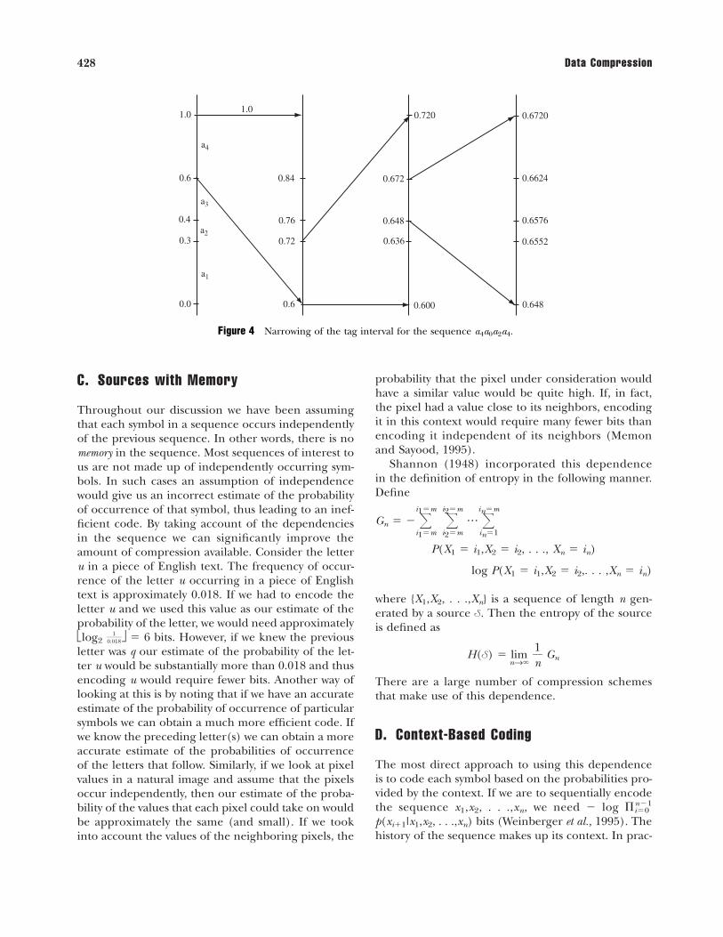
If the data we are attempting to compress consists ofnumerical values, such as images, using context-basedapproaches directly can be problematic. There areseveral reasons for this. Most context-based schemesexploit exact reoccurrence of patterns. Images areusually acquired using sensors that have a smallamount of noise. While this noise may not be per-ceptible, it is sufficient to reduce the occurrence ofexact repetitions of patterns. A simple alternative tousing the context approach is to generate a predic-tion for the value to be encoded and encode the pre-diction error. If there is considerable dependenceamong the values with high probability, the predic-tion will be close to the actual value and the predic-tion error will be a small number. We can encode thissmall number, which as it occurs with high probabil-ity will require fewer bits to encode. An example ofthis is shown in Fig. 5. The plot on the left of Fig. 5 isthe histogram of the pixel values of the sensin image,while the plot on the right is the histogram of the dif-ferences between neighboring pixels. We can see thatthe small differences occur much more frequentlyand therefore can be encoded using fewer bits. As


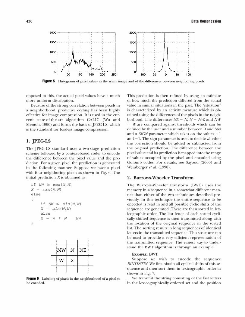
opposed to this, the actual pixel values have a muchmore uniform distribution.

Because of the strong correlation between pixels ina neighborhood, predictive coding has been highlyeffective for image compression. It is used in the cur-rent state-of-the-art algorithm CALIC (Wu andMemon, 1996) and forms the basis of JPEG-LS, whichis the standard for lossless image compression.

1. JPEG-LS

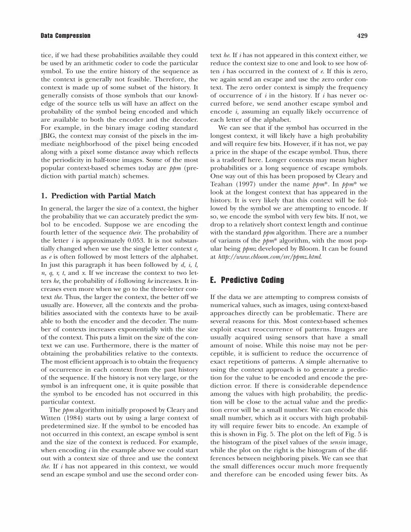
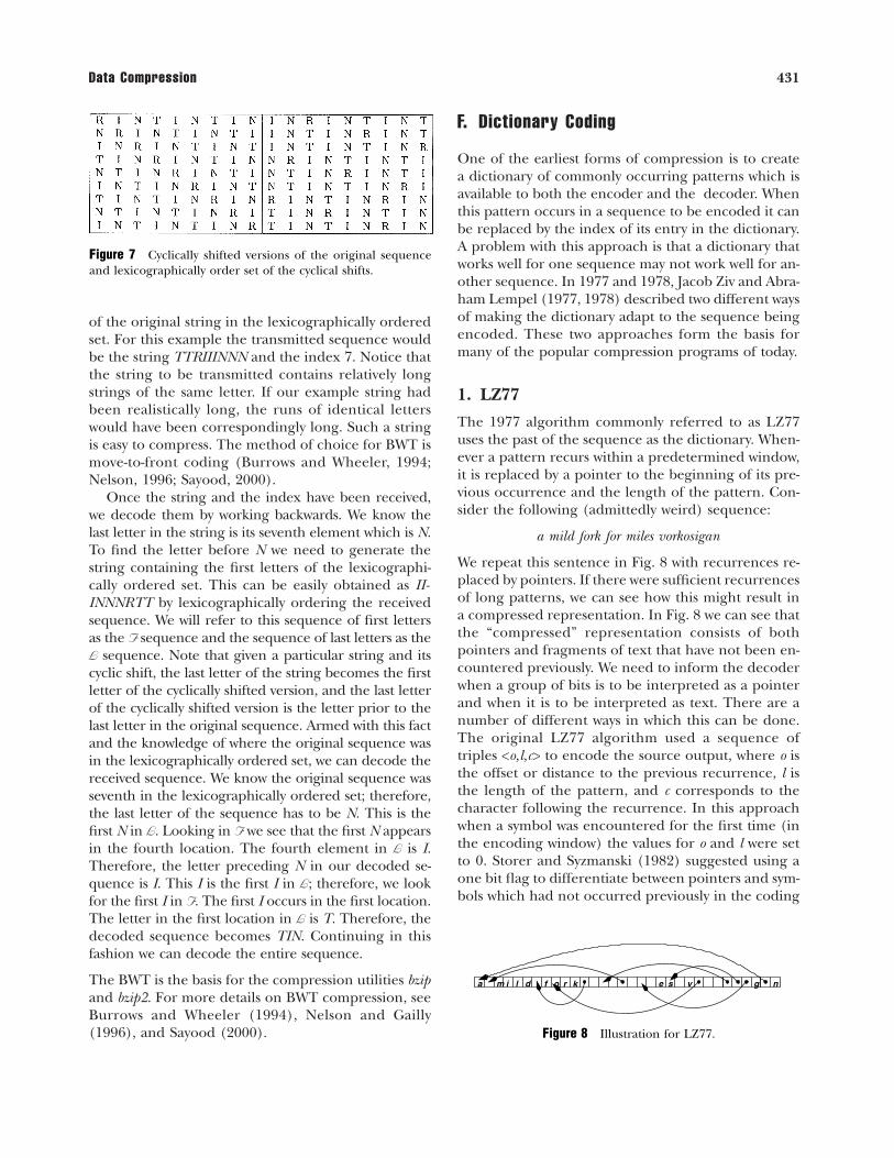
The JPEG-LS standard uses a two-stage predictionscheme followed by a context-based coder to encodethe difference between the pixel value and the pre-diction. For a given pixel the prediction is generatedin the following manner. Suppose we have a pixelwith four neighboring pixels as shown in Fig. 6. Theinitial prediction X is obtained as

if NW � max(W,N)X � max(W,N)else{

if NW � min(W,N)X � min(W,N)elseX � W � N � NW

}

This prediction is then refined by using an estimateof how much the prediction differed from the actualvalue in similar situations in the past. The “situation”is characterized by an activity measure which is ob-tained using the differences of the pixels in the neigh-borhood. The differences NE � N, N � NW, and NW� W are compared against thresholds which can bedefined by the user and a number between 0 and 364and a SIGN parameter which takes on the values �1and �1. The sign parameter is used to decide whetherthe correction should be added or subtracted fromthe original prediction. The difference between thepixel value and its prediction is mapped into the rangeof values occupied by the pixel and encoded usingGolomb codes. For details, see Sayood (2000) andWeinberger et al. (1998).

2. Burrows-Wheeler Transform

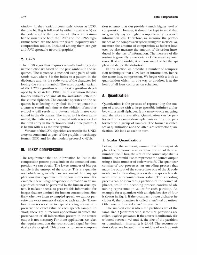
The Burrows-Wheeler transform (BWT) uses thememory in a sequence in a somewhat different man-ner than either of the two techniques described pre-viously. In this technique the entire sequence to beencoded is read in and all possible cyclic shifts of thesequence are generated. These are then sorted in lex-icographic order. The last letter of each sorted cycli-cally shifted sequence is then transmitted along withthe location of the original sequence in the sortedlist. The sorting results in long sequences of identicalletters in the transmitted sequence. This structure canbe used to provide a very efficient representation ofthe transmitted sequence. The easiest way to under-stand the BWT algorithm is through an example.

EXAMPLE: BWTSuppose we wish to encode the sequence

RINTINTIN. We first obtain all cyclical shifts of this se-quence and then sort them in lexicographic order asshown in Fig. 7.

We transmit the string consisting of the last lettersin the lexicographically ordered set and the position


Figure 5 Histograms of pixel values in the sensin image and of the differences between neighboring pixels.

Figure 6 Labeling of pixels in the neighborhood of a pixel tobe encoded.

of the original string in the lexicographically orderedset. For this example the transmitted sequence wouldbe the string TTRIIINNN and the index 7. Notice thatthe string to be transmitted contains relatively longstrings of the same letter. If our example string hadbeen realistically long, the runs of identical letterswould have been correspondingly long. Such a stringis easy to compress. The method of choice for BWT ismove-to-front coding (Burrows and Wheeler, 1994;Nelson, 1996; Sayood, 2000).

Once the string and the index have been received,we decode them by working backwards. We know thelast letter in the string is its seventh element which is N.To find the letter before N we need to generate thestring containing the first letters of the lexicographi-cally ordered set. This can be easily obtained as II-INNNRTT by lexicographically ordering the receivedsequence. We will refer to this sequence of first lettersas the F sequence and the sequence of last letters as theL sequence. Note that given a particular string and itscyclic shift, the last letter of the string becomes the firstletter of the cyclically shifted version, and the last letterof the cyclically shifted version is the letter prior to thelast letter in the original sequence. Armed with this factand the knowledge of where the original sequence wasin the lexicographically ordered set, we can decode thereceived sequence. We know the original sequence wasseventh in the lexicographically ordered set; therefore,the last letter of the sequence has to be N. This is thefirst N in L. Looking in F we see that the first N appearsin the fourth location. The fourth element in L is I.Therefore, the letter preceding N in our decoded se-quence is I. This I is the first I in L; therefore, we lookfor the first I in F. The first I occurs in the first location.The letter in the first location in L is T. Therefore, thedecoded sequence becomes TIN. Continuing in thisfashion we can decode the entire sequence.

The BWT is the basis for the compression utilities bzipand bzip2. For more details on BWT compression, seeBurrows and Wheeler (1994), Nelson and Gailly(1996), and Sayood (2000).

F. Dictionary Coding

One of the earliest forms of compression is to createa dictionary of commonly occurring patterns which isavailable to both the encoder and the decoder. Whenthis pattern occurs in a sequence to be encoded it canbe replaced by the index of its entry in the dictionary.A problem with this approach is that a dictionary thatworks well for one sequence may not work well for an-other sequence. In 1977 and 1978, Jacob Ziv and Abra-ham Lempel (1977, 1978) described two different waysof making the dictionary adapt to the sequence beingencoded. These two approaches form the basis formany of the popular compression programs of today.

1. LZ77

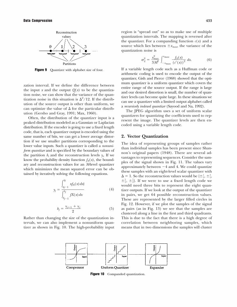
The 1977 algorithm commonly referred to as LZ77uses the past of the sequence as the dictionary. When-ever a pattern recurs within a predetermined window,it is replaced by a pointer to the beginning of its pre-vious occurrence and the length of the pattern. Con-sider the following (admittedly weird) sequence:

a mild fork for miles vorkosigan

We repeat this sentence in Fig. 8 with recurrences re-placed by pointers. If there were sufficient recurrencesof long patterns, we can see how this might result ina compressed representation. In Fig. 8 we can see thatthe “compressed” representation consists of bothpointers and fragments of text that have not been en-countered previously. We need to inform the decoderwhen a group of bits is to be interpreted as a pointerand when it is to be interpreted as text. There are anumber of different ways in which this can be done.The original LZ77 algorithm used a sequence oftriples <o,l,c> to encode the source output, where o isthe offset or distance to the previous recurrence, l isthe length of the pattern, and c corresponds to thecharacter following the recurrence. In this approachwhen a symbol was encountered for the first time (inthe encoding window) the values for o and l were setto 0. Storer and Syzmanski (1982) suggested using aone bit flag to differentiate between pointers and sym-bols which had not occurred previously in the coding


Figure 7 Cyclically shifted versions of the original sequenceand lexicographically order set of the cyclical shifts.

m i l d f o r k e s v g na

Figure 8 Illustration for LZ77.

window. In their variant, commonly known as LZSS,the one bit flag is followed by either a pair (<o,l>) orthe code word of the new symbol. There are a num-ber of variants of both the LZ77 and the LZSS algo-rithms which are the basis for several popularly usedcompression utilities. Included among them are gzipand PNG (portable network graphics).

2. LZ78

The 1978 algorithm requires actually building a dy-namic dictionary based on the past symbols in the se-quence. The sequence is encoded using pairs of codewords <i,c>, where i is the index to a pattern in thedictionary and c is the code word of the character fol-lowing the current symbol. The most popular variantof the LZ78 algorithm is the LZW algorithm devel-oped by Terry Welch (1984). In this variation the dic-tionary initially contains all the individual letters ofthe source alphabet. The encoder operates on the se-quence by collecting the symbols in the sequence intoa pattern p until such time as the addition of anothersymbol will result in a pattern which is not con-tained in the dictionary. The index to p is then trans-mitted, the pattern p concatenated with is added asthe next entry in the dictionary, and a new pattern pis begun with as the first symbol.

Variants of the LZW algorithm are used in the UNIXcompress command as part of the graphic interchangeformat (GIF) and for the modem protocol v. 42bis.

III. LOSSY COMPRESSION

The requirement that no information be lost in thecompression process puts a limit on the amount of com-pression we can obtain. The lowest number of bits persample is the entropy of the source. This is a quantityover which we generally have no control. In many ap-plications this requirement of no loss is excessive. Forexample, there is high-frequency information in an im-age which cannot be perceived by the human visual sys-tem. It makes no sense to preserve this information forimages that are destined for human consumption. Sim-ilarly, when we listen to sampled speech we cannot per-ceive the exact numerical value of each sample. There-fore, it makes no sense to expend coding resources topreserve the exact value of each speech sample. Inshort, there are numerous applications in which thepreservation of all information present in the sourceoutput is not necessary. For these applications we relaxthe requirement that the reconstructed signal be iden-tical to the original. This allows us to create compres-

sion schemes that can provide a much higher level ofcompression. However, it should be kept in mind thatwe generally pay for higher compression by increasedinformation loss. Therefore, we measure the perfor-mance of the compression system using two metrics. Wemeasure the amount of compression as before; how-ever, we also measure the amount of distortion intro-duced by the loss of information. The measure of dis-tortion is generally some variant of the mean squarederror. If at all possible, it is more useful to let the ap-plication define the distortion.

In this section we describe a number of compres-sion techniques that allow loss of information, hencethe name lossy compression. We begin with a look atquantization which, in one way or another, is at theheart of all lossy compression schemes.

A. Quantization

Quantization is the process of representing the out-put of a source with a large (possibly infinite) alpha-bet with a small alphabet. It is a many-to-one mappingand therefore irreversible. Quantization can be per-formed on a sample-by-sample basis or it can be per-formed on a group of samples. The former is calledscalar quantization and the latter is called vector quan-tization. We look at each in turn.

1. Scalar Quantization

Let us, for the moment, assume that the output al-phabet of the source is all or some portion of the realnumber line. Thus, the size of the source alphabet isinfinite. We would like to represent the source outputusing a finite number of code words M. The quantizerconsists of two processes: an encoding process thatmaps the output of the source into one of the M codewords, and a decoding process that maps each codeword into a reconstruction value. The encodingprocess can be viewed as a partition of the source al-phabet, while the decoding process consists of ob-taining representation values for each partition. Anexample for a quantizer with an alphabet size of fouris shown in Fig. 9. If the quantizer output alphabet in-cludes 0, the quantizer is called a midtread quantizer.Otherwise, it is called a midrise quantizer.

The simplest case is when the partitions are of thesame size. Quantizers with same size partitions arecalled uniform quantizers. If the source is uniformly dis-tributed between �A and A, the size of the partitionor quantization interval � is 2A/M. The reconstruc-tion values are located in the middle of each quanti-


zation interval. If we define the difference betweenthe input x and the output Q(x) to be the quantiza-tion noise, we can show that the variance of the quan-tization noise in this situation is �2/12. If the distrib-ution of the source output is other than uniform, wecan optimize the value of � for the particular distrib-ution (Gersho and Gray, 1991; Max, 1960).

Often, the distribution of the quantizer input is apeaked distribution modeled as a Gaussian or Laplaciandistribution. If the encoder is going to use a fixed lengthcode, that is, each quantizer output is encoded using thesame number of bits, we can get a lower average distor-tion if we use smaller partitions corresponding to thelower value inputs. Such a quantizer is called a nonuni-form quantizer and is specified by the boundary values ofthe partition bi and the reconstruction levels yi. If weknow the probability density function fX(x), the bound-ary and reconstruction values for an M-level quantizerwhich minimizes the mean squared error can be ob-tained by iteratively solving the following equations.

yj �

�bj

bj�1xfX(x)dx}

�bj

bj�1fX(x)dx

(4)

bj � (5)

Rather than changing the size of the quantization in-tervals, we can also implement a nonuniform quan-tizer as shown in Fig. 10. The high-probability input

yj�1 � yj�2

region is “spread out” so as to make use of multiplequantization intervals. The mapping is reversed afterthe quantizer. For a companding function c(x) and asource which lies between �xmax, the variance of thequantization noise is

�q2 � �xmax

�xmaxdx. (6)

If a variable length code such as a Huffman code orarithmetic coding is used to encode the output of thequantizer, Gish and Pierce (1968) showed that the opti-mum quantizer is a uniform quantizer which covers theentire range of the source output. If the range is largeand our desired distortion is small, the number of quan-tizer levels can become quite large. In these situations wecan use a quantizer with a limited output alphabet calleda recursively indexed quantizer (Sayood and Na, 1992).

The JPEG algorithm uses a set of uniform scalarquantizers for quantizing the coefficients used to rep-resent the image. The quantizer levels are then en-coded using a variable length code.

2. Vector Quantization

The idea of representing groups of samples ratherthan individual samples has been present since Shan-non’s original papers (1948). There are several ad-vantages to representing sequences. Consider the sam-ples of the signal shown in Fig. 11. The values varyapproximately between �4 and 4. We could quantizethese samples with an eight-level scalar quantizer with� � 1. So the reconstruction values would be {��

12

�, ��32

�,��

52

�, ��72

�}. If we were to use a fixed length code wewould need three bits to represent the eight quan-tizer outputs. If we look at the output of the quantizerin pairs, we get 64 possible reconstruction values.These are represented by the larger filled circles inFig. 12. However, if we plot the samples of the signalas pairs (as in Fig. 13) we see that the samples areclustered along a line in the first and third quadrants.This is due to the fact that there is a high degree ofcorrelation between neighboring samples, whichmeans that in two dimensions the samples will cluster

fX(x)�(c�(x))2

x2max�

3M2


Reconstructionvalues

Partitions

Figure 9 Quantizer with alphabet size of four.

Figure 10 Companded quantization.

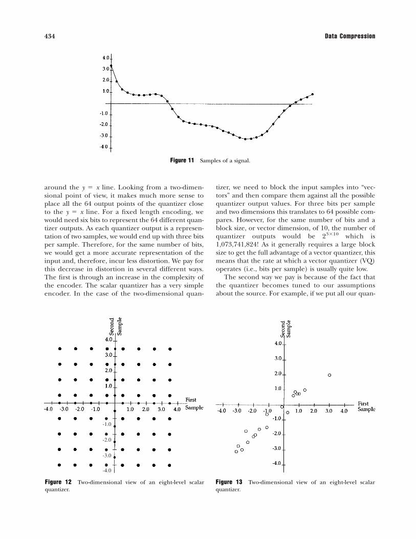
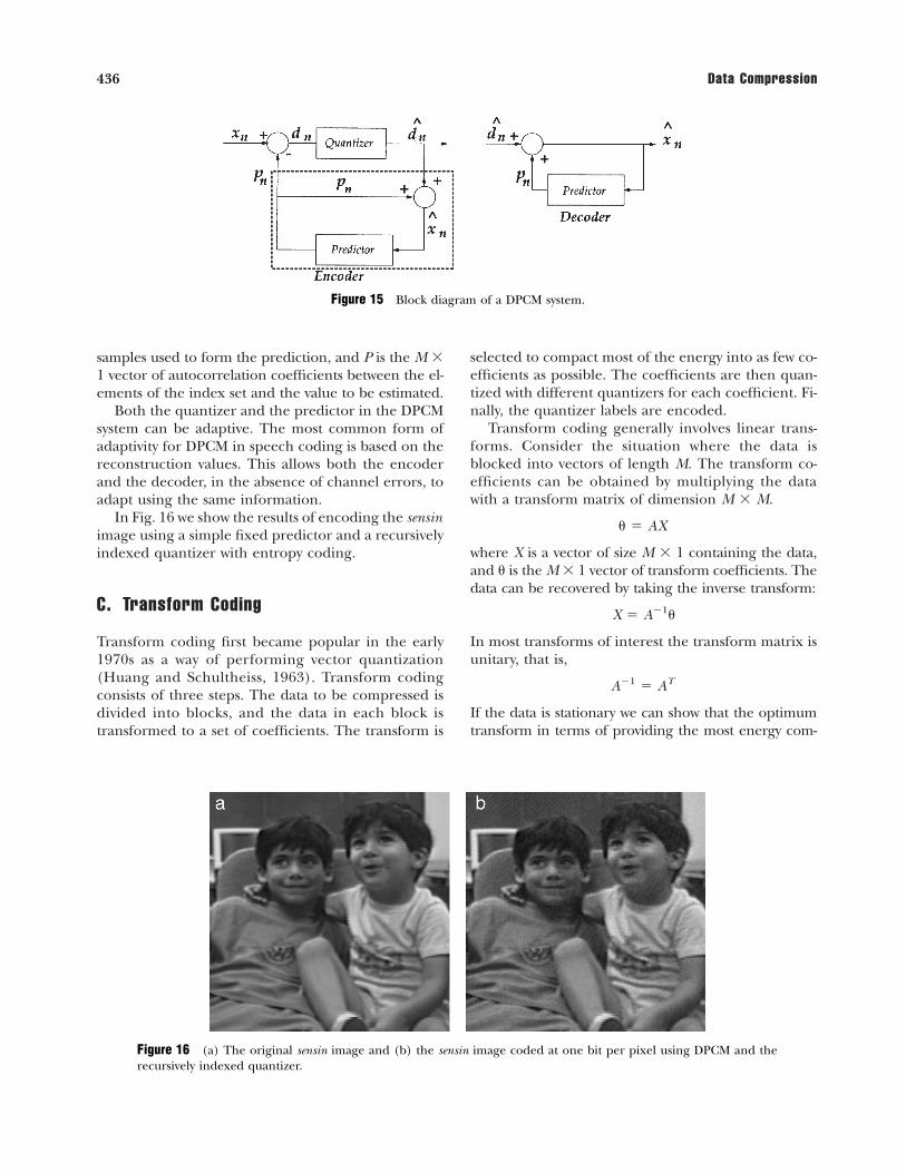
around the y � x line. Looking from a two-dimen-sional point of view, it makes much more sense toplace all the 64 output points of the quantizer closeto the y � x line. For a fixed length encoding, wewould need six bits to represent the 64 different quan-tizer outputs. As each quantizer output is a represen-tation of two samples, we would end up with three bitsper sample. Therefore, for the same number of bits,we would get a more accurate representation of theinput and, therefore, incur less distortion. We pay forthis decrease in distortion in several different ways.The first is through an increase in the complexity ofthe encoder. The scalar quantizer has a very simpleencoder. In the case of the two-dimensional quan-

tizer, we need to block the input samples into “vec-tors” and then compare them against all the possiblequantizer output values. For three bits per sampleand two dimensions this translates to 64 possible com-pares. However, for the same number of bits and ablock size, or vector dimension, of 10, the number ofquantizer outputs would be 2310 which is1,073,741,824! As it generally requires a large blocksize to get the full advantage of a vector quantizer, thismeans that the rate at which a vector quantizer (VQ)operates (i.e., bits per sample) is usually quite low.

The second way we pay is because of the fact thatthe quantizer becomes tuned to our assumptionsabout the source. For example, if we put all our quan-


Figure 11 Samples of a signal.

-1.0

-2.0

-3.0

-4.0

Figure 12 Two-dimensional view of an eight-level scalar quantizer.

Figure 13 Two-dimensional view of an eight-level scalar quantizer.

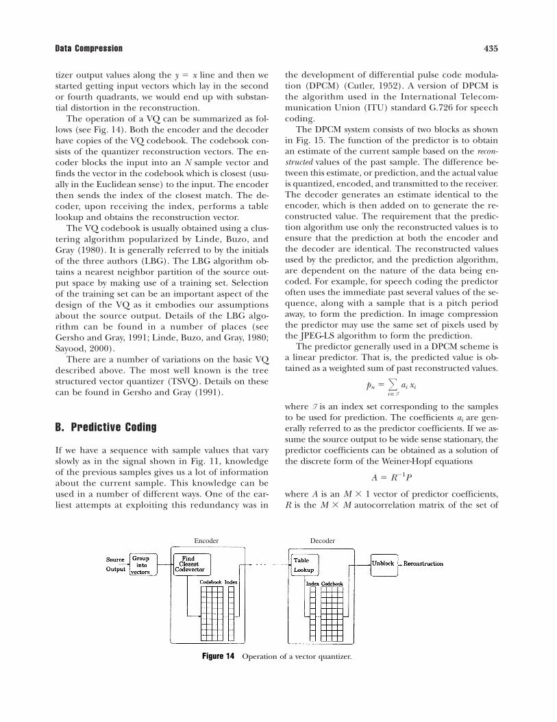
tizer output values along the y � x line and then westarted getting input vectors which lay in the secondor fourth quadrants, we would end up with substan-tial distortion in the reconstruction.

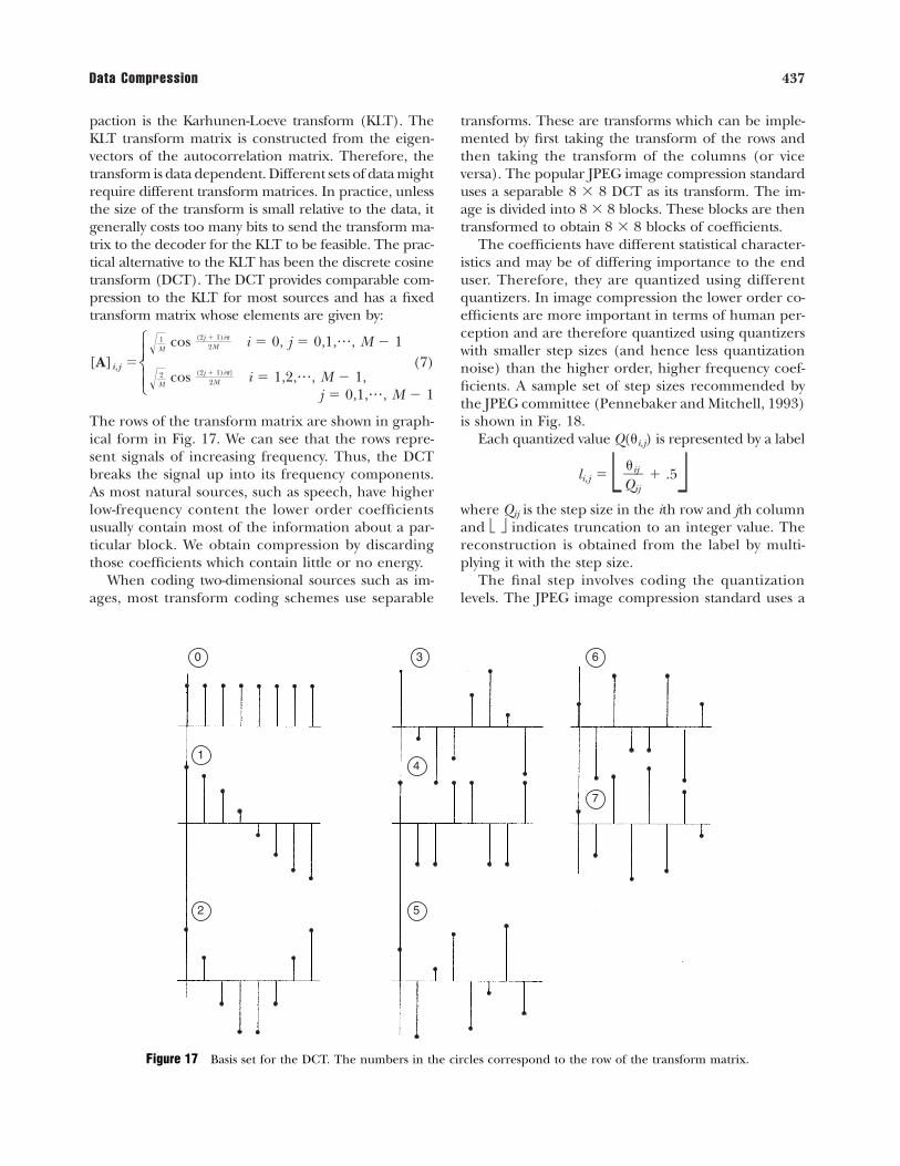
The operation of a VQ can be summarized as fol-lows (see Fig. 14). Both the encoder and the decoderhave copies of the VQ codebook. The codebook con-sists of the quantizer reconstruction vectors. The en-coder blocks the input into an N sample vector andfinds the vector in the codebook which is closest (usu-ally in the Euclidean sense) to the input. The encoderthen sends the index of the closest match. The de-coder, upon receiving the index, performs a tablelookup and obtains the reconstruction vector.

The VQ codebook is usually obtained using a clus-tering algorithm popularized by Linde, Buzo, andGray (1980). It is generally referred to by the initialsof the three authors (LBG). The LBG algorithm ob-tains a nearest neighbor partition of the source out-put space by making use of a training set. Selectionof the training set can be an important aspect of thedesign of the VQ as it embodies our assumptionsabout the source output. Details of the LBG algo-rithm can be found in a number of places (see Gersho and Gray, 1991; Linde, Buzo, and Gray, 1980;Sayood, 2000).

There are a number of variations on the basic VQdescribed above. The most well known is the treestructured vector quantizer (TSVQ). Details on thesecan be found in Gersho and Gray (1991).

B. Predictive Coding

If we have a sequence with sample values that varyslowly as in the signal shown in Fig. 11, knowledgeof the previous samples gives us a lot of informationabout the current sample. This knowledge can beused in a number of different ways. One of the ear-liest attempts at exploiting this redundancy was in

the development of differential pulse code modula-tion (DPCM) (Cutler, 1952). A version of DPCM isthe algorithm used in the International Telecom-munication Union (ITU) standard G.726 for speechcoding.

The DPCM system consists of two blocks as shownin Fig. 15. The function of the predictor is to obtainan estimate of the current sample based on the recon-structed values of the past sample. The difference be-tween this estimate, or prediction, and the actual valueis quantized, encoded, and transmitted to the receiver.The decoder generates an estimate identical to theencoder, which is then added on to generate the re-constructed value. The requirement that the predic-tion algorithm use only the reconstructed values is toensure that the prediction at both the encoder andthe decoder are identical. The reconstructed valuesused by the predictor, and the prediction algorithm,are dependent on the nature of the data being en-coded. For example, for speech coding the predictoroften uses the immediate past several values of the se-quence, along with a sample that is a pitch periodaway, to form the prediction. In image compressionthe predictor may use the same set of pixels used bythe JPEG-LS algorithm to form the prediction.

The predictor generally used in a DPCM scheme isa linear predictor. That is, the predicted value is ob-tained as a weighted sum of past reconstructed values.

pn � �i�I

ai xi

where I is an index set corresponding to the samplesto be used for prediction. The coefficients ai are gen-erally referred to as the predictor coefficients. If we as-sume the source output to be wide sense stationary, thepredictor coefficients can be obtained as a solution ofthe discrete form of the Weiner-Hopf equations

A � R�1P

where A is an M 1 vector of predictor coefficients, R is the M M autocorrelation matrix of the set of


Encoder Decoder

Figure 14 Operation of a vector quantizer.

samples used to form the prediction, and P is the M 1 vector of autocorrelation coefficients between the el-ements of the index set and the value to be estimated.

Both the quantizer and the predictor in the DPCMsystem can be adaptive. The most common form ofadaptivity for DPCM in speech coding is based on thereconstruction values. This allows both the encoderand the decoder, in the absence of channel errors, toadapt using the same information.

In Fig. 16 we show the results of encoding the sensinimage using a simple fixed predictor and a recursivelyindexed quantizer with entropy coding.

C. Transform Coding

Transform coding first became popular in the early1970s as a way of performing vector quantization(Huang and Schultheiss, 1963). Transform codingconsists of three steps. The data to be compressed isdivided into blocks, and the data in each block istransformed to a set of coefficients. The transform is

selected to compact most of the energy into as few co-efficients as possible. The coefficients are then quan-tized with different quantizers for each coefficient. Fi-nally, the quantizer labels are encoded.

Transform coding generally involves linear trans-forms. Consider the situation where the data isblocked into vectors of length M. The transform co-efficients can be obtained by multiplying the datawith a transform matrix of dimension M M.

� � AX

where X is a vector of size M 1 containing the data,and � is the M 1 vector of transform coefficients. Thedata can be recovered by taking the inverse transform:

X � A�1�

In most transforms of interest the transform matrix isunitary, that is,

A�1 � AT

If the data is stationary we can show that the optimumtransform in terms of providing the most energy com-


Figure 15 Block diagram of a DPCM system.

Figure 16 (a) The original sensin image and (b) the sensin image coded at one bit per pixel using DPCM and therecursively indexed quantizer.

paction is the Karhunen-Loeve transform (KLT). TheKLT transform matrix is constructed from the eigen-vectors of the autocorrelation matrix. Therefore, thetransform is data dependent. Different sets of data mightrequire different transform matrices. In practice, unlessthe size of the transform is small relative to the data, itgenerally costs too many bits to send the transform ma-trix to the decoder for the KLT to be feasible. The prac-tical alternative to the KLT has been the discrete cosinetransform (DCT). The DCT provides comparable com-pression to the KLT for most sources and has a fixedtransform matrix whose elements are given by:

[A]i,j ��

M1�� cos �(2j �

2M1)i�� i � 0, j � 0,1,, M � 1

��M2�� cos �(2j �

2M1)i�}� i � 1,2,, M � 1,

(7)

j � 0,1,, M � 1

The rows of the transform matrix are shown in graph-ical form in Fig. 17. We can see that the rows repre-sent signals of increasing frequency. Thus, the DCTbreaks the signal up into its frequency components.As most natural sources, such as speech, have higherlow-frequency content the lower order coefficientsusually contain most of the information about a par-ticular block. We obtain compression by discardingthose coefficients which contain little or no energy.

When coding two-dimensional sources such as im-ages, most transform coding schemes use separable

transforms. These are transforms which can be imple-mented by first taking the transform of the rows andthen taking the transform of the columns (or viceversa). The popular JPEG image compression standarduses a separable 8 8 DCT as its transform. The im-age is divided into 8 8 blocks. These blocks are thentransformed to obtain 8 8 blocks of coefficients.

The coefficients have different statistical character-istics and may be of differing importance to the enduser. Therefore, they are quantized using differentquantizers. In image compression the lower order co-efficients are more important in terms of human per-ception and are therefore quantized using quantizerswith smaller step sizes (and hence less quantizationnoise) than the higher order, higher frequency coef-ficients. A sample set of step sizes recommended bythe JPEG committee (Pennebaker and Mitchell, 1993)is shown in Fig. 18.

Each quantized value Q(�i,j) is represented by a label

li,j � � .5where Qij is the step size in the ith row and jth columnand indicates truncation to an integer value. Thereconstruction is obtained from the label by multi-plying it with the step size.

The final step involves coding the quantization levels. The JPEG image compression standard uses a

�ij�Qij


0 3 6

7

41

2 5

Figure 17 Basis set for the DCT. The numbers in the circles correspond to the row of the transform matrix.

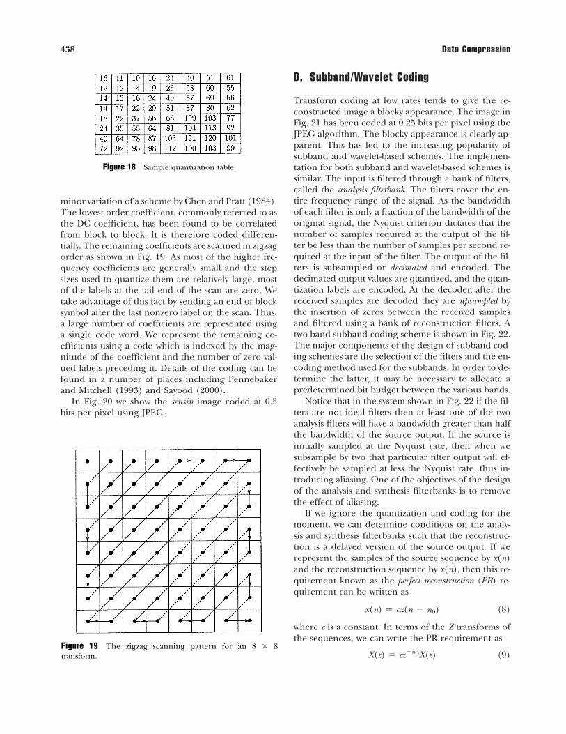
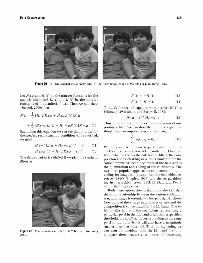
minor variation of a scheme by Chen and Pratt (1984).The lowest order coefficient, commonly referred to asthe DC coefficient, has been found to be correlatedfrom block to block. It is therefore coded differen-tially. The remaining coefficients are scanned in zigzagorder as shown in Fig. 19. As most of the higher fre-quency coefficients are generally small and the stepsizes used to quantize them are relatively large, mostof the labels at the tail end of the scan are zero. Wetake advantage of this fact by sending an end of blocksymbol after the last nonzero label on the scan. Thus,a large number of coefficients are represented usinga single code word. We represent the remaining co-efficients using a code which is indexed by the mag-nitude of the coefficient and the number of zero val-ued labels preceding it. Details of the coding can befound in a number of places including Pennebakerand Mitchell (1993) and Sayood (2000).

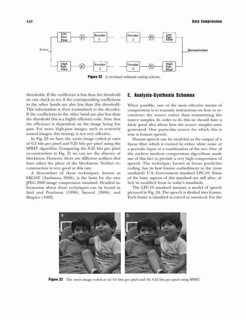
In Fig. 20 we show the sensin image coded at 0.5bits per pixel using JPEG.

D. Subband/Wavelet Coding

Transform coding at low rates tends to give the re-constructed image a blocky appearance. The image inFig. 21 has been coded at 0.25 bits per pixel using theJPEG algorithm. The blocky appearance is clearly ap-parent. This has led to the increasing popularity ofsubband and wavelet-based schemes. The implemen-tation for both subband and wavelet-based schemes issimilar. The input is filtered through a bank of filters,called the analysis filterbank. The filters cover the en-tire frequency range of the signal. As the bandwidthof each filter is only a fraction of the bandwidth of theoriginal signal, the Nyquist criterion dictates that thenumber of samples required at the output of the fil-ter be less than the number of samples per second re-quired at the input of the filter. The output of the fil-ters is subsampled or decimated and encoded. Thedecimated output values are quantized, and the quan-tization labels are encoded. At the decoder, after thereceived samples are decoded they are upsampled bythe insertion of zeros between the received samplesand filtered using a bank of reconstruction filters. Atwo-band subband coding scheme is shown in Fig. 22.The major components of the design of subband cod-ing schemes are the selection of the filters and the en-coding method used for the subbands. In order to de-termine the latter, it may be necessary to allocate apredetermined bit budget between the various bands.

Notice that in the system shown in Fig. 22 if the fil-ters are not ideal filters then at least one of the twoanalysis filters will have a bandwidth greater than halfthe bandwidth of the source output. If the source isinitially sampled at the Nyquist rate, then when wesubsample by two that particular filter output will ef-fectively be sampled at less the Nyquist rate, thus in-troducing aliasing. One of the objectives of the designof the analysis and synthesis filterbanks is to removethe effect of aliasing.

If we ignore the quantization and coding for themoment, we can determine conditions on the analy-sis and synthesis filterbanks such that the reconstruc-tion is a delayed version of the source output. If werepresent the samples of the source sequence by x(n)and the reconstruction sequence by x(n), then this re-quirement known as the perfect reconstruction (PR) re-quirement can be written as

x(n) � cx(n � n0) (8)

where c is a constant. In terms of the Z transforms ofthe sequences, we can write the PR requirement as

X(z) � cz�n0X(z) (9)


Figure 18 Sample quantization table.

Figure 19 The zigzag scanning pattern for an 8 8 transform.

Let H1(z) and H2(z) be the transfer functions for theanalysis filters and K1(z) and K2(z) be the transferfunctions of the synthesis filters. Then we can show(Sayood, 2000) that

X(z) � �12

� [H1(z)K1(z) � H2(z)K2(z)]X(z)

� �12

� [H1(�z)K1(z) � H2(�z)K2(z)]X(�z) (10)

Examining this equation we can see that in order forthe perfect reconstruction condition to be satisfied,we need

H1(�z)K1(z) � H2(�z)K2(z) � 0 (11)

H1(z)K1(z) � H2(z)K2(z) � cz�n0 (12)

The first equation is satisfied if we pick the synthesisfilters as

K1(z) � �H2(z) (13)

K2(z) � H1(�z) (14)

To satisfy the second equation we can select H2(z) as(Mintzer, 1985; Smith and Barnwell, 1984)

H2(z) � z�N H1(�z�1) (15)

Thus, all four filters can be expressed in terms of oneprototype filter. We can show that this prototype filtershould have an impulse response satisfying

�N

k�0hkhk�2n � �n (16)

We can arrive at the same requirement on the filtercoefficients using a wavelet formulation. Once wehave obtained the coefficients for the filters, the com-pression approach using wavelets is similar. After thesource output has been decomposed the next step isthe quantization and coding of the coefficients. Thetwo most popular approaches to quantization andcoding for image compression are the embedded ze-rotree (EZW) (Shapiro, 1993) and the set partition-ing in hierarchical trees (SPIHT) (Said and Pearl-man, 1996) approaches.

Both these approaches make use of the fact thatthere is a relationship between the various subbands.A natural image is essentially a low-pass signal. There-fore, most of the energy in a wavelet or subband de-composition is concentrated in the LL band. One ef-fect of this is that if the coefficient representing aparticular pixel in the LL band is less than a specifiedthreshold, the coefficients corresponding to the samepixel in the other bands will also have a magnitudesmaller than that threshold. Thus, during coding wecan scan the coefficients in the LL band first andcompare them against a sequence of decreasing


Figure 20 (a) The original sensin image and (b) the sensin image coded at 0.5 bits per pixel using JPEG.

Figure 21 The sensin image coded at 0.25 bits per pixel usingJPEG.

thresholds. If the coefficient is less than the thresholdwe can check to see if the corresponding coefficientsin the other bands are also less than this threshold.This information is then transmitted to the decoder.If the coefficients in the other band are also less thanthe threshold this is a highly efficient code. Note thatthe efficiency is dependent on the image being lowpass. For more high-pass images, such as remotelysensed images, this strategy is not very effective.

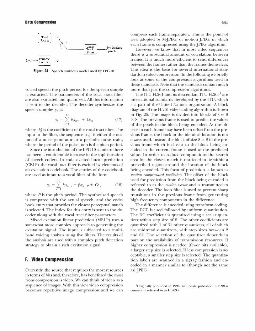
In Fig. 23 we have the sensin image coded at ratesof 0.5 bits per pixel and 0.25 bits per pixel using theSPIHT algorithm. Comparing the 0.25 bits per pixelreconstruction to Fig. 21 we can see the absence ofblockiness. However, there are different artifacts thathave taken the place of the blockiness. Neither re-construction is very good at this rate.

A descendant of these techniques, known asEBCOT (Taubman, 2000), is the basis for the newJPEG 2000 image compression standard. Detailed in-formation about these techniques can be found inSaid and Pearlman (1996), Sayood (2000), andShapiro (1993).

E. Analysis-Synthesis Schemes

When possible, one of the most effective means ofcompression is to transmit instructions on how to re-construct the source rather than transmitting thesource samples. In order to do this we should have afairly good idea about how the source samples weregenerated. One particular source for which this istrue is human speech.

Human speech can be modeled as the output of alinear filter which is excited by either white noise ora periodic input or a combination of the two. One ofthe earliest modern compression algorithms madeuse of this fact to provide a very high compression ofspeech. The technique, known as linear predictivecoding, has its best known embodiment in the (nowoutdated) U.S. Government standard LPC-10. Someof the basic aspects of this standard are still alive, al-beit in modified form in today’s standards.

The LPC-10 standard assumes a model of speechpictured in Fig. 24. The speech is divided into frames.Each frame is classified as voiced or unvoiced. For the


Source

Figure 22 A two-band subband coding scheme.

Figure 23 The sensin image coded at (a) 0.5 bits per pixel and (b) 0.25 bits per pixel using SPIHT.

voiced speech the pitch period for the speech sampleis extracted. The parameters of the vocal tract filterare also extracted and quantized. All this informationis sent to the decoder. The decoder synthesizes thespeech samples yn as

yn � �M

i�1biyn�i � G�n (17)

where {bi} is the coefficient of the vocal tract filter. Theinput to the filter, the sequence {�n}, is either the out-put of a noise generator or a periodic pulse train,where the period of the pulse train is the pitch period.

Since the introduction of the LPC-10 standard therehas been a considerable increase in the sophisticationof speech coders. In code excited linear prediction(CELP) the vocal tract filter is excited by elements ofan excitation codebook. The entries of the codebookare used as input to a vocal filter of the form

yn � �10

i�1biyn�i � �yn�P � G�n (18)

where P is the pitch period. The synthesized speechis compared with the actual speech, and the code-book entry that provides the closest perceptual matchis selected. The index for this entry is sent to the de-coder along with the vocal tract filter parameters.

Mixed excitation linear prediction (MELP) uses asomewhat more complex approach to generating theexcitation signal. The input is subjected to a multi-band voicing analysis using five filters. The results ofthe analysis are used with a complex pitch detectionstrategy to obtain a rich excitation signal.

F. Video Compression

Currently, the source that requires the most resourcesin terms of bits and, therefore, has benefitted the mostfrom compression is video. We can think of video as asequence of images. With this view video compressionbecomes repetitive image compression and we can

compress each frame separately. This is the point ofview adopted by M-JPEG, or motion JPEG, in whicheach frame is compressed using the JPEG algorithm.

However, we know that in most video sequencesthere is a substantial amount of correlation betweenframes. It is much more efficient to send differencesbetween the frames rather than the frames themselves.This idea is the basis for several international stan-dards in video compression. In the following we brieflylook at some of the compression algorithms used inthese standards. Note that the standards contain muchmore than just the compression algorithms.

The ITU H.261 and its descendant ITU H.2631 areinternational standards developed by the ITU, whichis a part of the United Nations organization. A blockdiagram of the H.261 video coding algorithm is shownin Fig. 25. The image is divided into blocks of size 8 8. The previous frame is used to predict the valuesof the pixels in the block being encoded. As the ob-jects in each frame may have been offset from the pre-vious frame, the block in the identical location is notalways used. Instead the block of size 8 8 in the pre-vious frame which is closest to the block being en-coded in the current frame is used as the predictedvalue. In order to reduce computations the searcharea for the closest match is restricted to lie within aprescribed region around the location of the blockbeing encoded. This form of prediction is known asmotion compensated prediction. The offset of the blockused for prediction from the block being encoded isreferred to as the motion vector and is transmitted tothe decoder. The loop filter is used to prevent sharptransitions in the previous frame from generatinghigh frequency components in the difference.

The difference is encoded using transform coding.The DCT is used followed by uniform quantization.The DC coefficient is quantized using a scalar quan-tizer with a step size of 8. The other coefficients arequantized with 1 of 31 other quantizers, all of whichare midtread quantizers, with step sizes between 2and 62. The selection of the quantizer depends inpart on the availability of transmission resources. Ifhigher compression is needed (fewer bits available),a larger step size is selected. If less compression is ac-ceptable, a smaller step size is selected. The quantiza-tion labels are scanned in a zigzag fashion and en-coded in a manner similar to (though not the sameas) JPEG.


Figure 24 Speech synthesis model used by LPC-10.

1Originally published in 1996; an update published in 1998 iscommonly referred to as H.263�.

The coding algorithm for ITU-T H.263 is similar tothat used for H.261 with some improvements. The im-provements include:

• Better motion compensated prediction• Better coding• Increased number of formats• Increased error resilience

There are a number of other improvements that arenot essential for the compression algorithm. As men-tioned before, there are two versions of H.263. As theearlier version is a subset of the latter one; we only de-scribe the later version.

The prediction is enhanced in H.263 in a numberof ways. By interpolating between neighboring pixelsin the frame being searched, a “larger image” is cre-ated. This essentially allows motion compensation dis-placement of half pixel steps rather than integer num-ber of pixels. There is an unrestricted motion vectormode that allows references to areas outside the pic-ture, where the outside areas are generated by dupli-cating the pixels at the image boundaries. Finally, inH.263� the prediction can be generated by a framethat is not the previous frame. An independent seg-ment decoding mode allows the frame to be brokeninto segments where each segment can be decodedindependently. This prevents error propagation and

also allows for greater control over quality of regionsin the reconstruction. The H.263 standard also allowsfor bidirectional prediction.

As the H.261 algorithm was designed for video-conferencing, there was no consideration given to theneed for random access. The MPEG standards incor-porate this need by requiring that at fixed intervals aframe of an image be encoded without reference topast frames. The MPEG-1 standard defines three dif-ferent kinds of frames: I frames, P frames, and Bframes. An I frame is coded without reference to pre-vious frames, that is, no use is made of predictionfrom previous frames. The use of the I frames allowsrandom access. If such frames did not exist in thevideo sequence, then to view any given frame we wouldhave to decompress all previous frames, as the recon-struction of each frame would be dependent on theprediction from previous frames. The use of periodicI frames is also necessary if the standard is to be usedfor compressing television programming. A viewershould have the ability to turn on the television (andthe MPEG decoder) at more or less any time duringthe broadcast. If there are periodic I frames available,then the decoder can start decoding from the first Iframe. Without the redundancy removal provided viaprediction the compression obtained with I frames isless than would have been possible if prediction hadbeen used.


Loop filterstatus

Motionvector

+

–

Figure 25 Block diagram of the ITU-T H.261 video compression algorithm.

The P frame is similar to frames in the H.261 stan-dard in that it is generated based on prediction fromprevious reconstructed frames. The similarity is closerto H.263, as the MPEG-1 standard allows for half pixelshifts during motion compensated prediction.

The B frame was introduced in the MPEG-1 stan-dard to offset the loss of compression efficiency occa-sioned by the I frames. The B frame is generated us-ing prediction from the previous P or I frame and thenearest future P or I frame. This results in extremelygood prediction and a high level of compression. TheB frames are not used to predict other frames, there-fore, the B frames can tolerate more error. This alsopermits higher levels of compression.

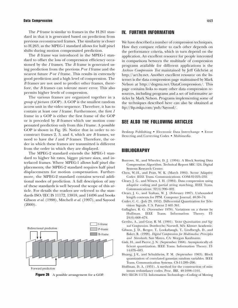
The various frames are organized together in agroup of pictures (GOP). A GOP is the smallest randomaccess unit in the video sequence. Therefore, it has tocontain at least one I frame. Furthermore, the first Iframe in a GOP is either the first frame of the GOPor is preceded by B frames which use motion com-pensated prediction only from this I frame. A possibleGOP is shown in Fig. 26. Notice that in order to re-construct frames 2, 3, and 4, which are B frames, weneed to have the I and P frames. Therefore, the or-der in which these frames are transmitted is differentfrom the order in which they are displayed.

The MPEG-2 standard extends the MPEG-1 stan-dard to higher bit rates, bigger picture sizes, and in-terlaced frames. Where MPEG-1 allows half pixel dis-placements, the MPEG-2 standard requires half pixeldisplacements for motion compensation. Further-more, the MPEG-2 standard contains several addi-tional modes of prediction. A full description of anyof these standards is well beyond the scope of this ar-ticle. For details the readers are referred to the stan-dards ISO/IEC IS 11172, 13818, and 14496 and booksGibson et al. (1998), Mitchell et al. (1997), and Sayood(2000).

IV. FURTHER INFORMATION

We have described a number of compression techniques.How they compare relative to each other depends onthe performance criteria, which in turn depend on theapplication. An excellent resource for people interestedin comparisons between the multitude of compressionprograms available for different applications is theArchive Compression Test maintained by Jeff Gilchrist athttp://act.by.net. Another excellent resource on the In-ternet is the data compression page maintained by MarkNelson at http://dogma.net/DataCompression/. Thispage contains links to many other data compression re-sources, including programs and a set of informative ar-ticles by Mark Nelson. Programs implementing some ofthe techniques described here can also be obtained atftp://ftp.mkp.com/pub/Sayood/.

SEE ALSO THE FOLLOWING ARTICLES

Desktop Publishing • Electronic Data Interchange • ErrorDetecting and Correcting Codes • Multimedia

BIBLIOGRAPHY

Burrows, M., and Wheeler, D. J. (1994). A Block Sorting DataCompression Algorithm. Technical Report SRC 124, DigitalSystems Research Center.

Chen, W.-H., and Pratt, W. K. (March 1984). Scene AdaptiveCoder. IEEE Trans. Communications. COM-32:225–232.

Cleary, J. G., and Witten, I. H. (1984). Data compression usingadaptive coding and partial string matching. IEEE Trans.Communications. 32(4):396–402.

Cleary, J. G., and Teahan, W. J. (February 1997). Unboundedlength contexts for PPM. Computer Journal, 40:30–74.

Cutler, C. C. (July 29, 1952). Differential Quantization for Tele-vision Signals. U.S. Patent 2 605 361.

Gallagher, R. G. (November 1978). Variations on a theme byHuffman. IEEE Trans. Information Theory. IT-24(6):668–674.

Gersho, A., and Gray, R. M. (1991). Vector Quantization and Sig-nal Compression. Dordrecht/Norwell, MA: Kluwer Academic.

Gibson, J. D., Berger, T., Lookabaugh, T., Lindbergh, D., andBaker, R. (1998). Digital Compression for Multimedia: Principlesand Standards. San Mateo, CA: Morgan Kaufmann.

Gish, H., and Pierce, J. N. (September 1968). Asymptotically ef-ficient quantization. IEEE Trans. Information Theory. IT-14:676–683.

Huang, J.-Y., and Schultheiss, P. M. (September 1963). Blockquantization of correlated gaussian random variables. IEEETrans. Communication Systems. CS-11:289–296.

Huffman, D. A. (1951). A method for the construction of min-imum redundancy codes. Proc. IRE. 40:1098–1101.

ISO/IECIS 11172. Information Technology—Coding of Moving


Bidirectional prediction

Forward prediction

I-frame

P-frame

B-frame

Figure 26 A possible arrangement for a GOP.

Pictures and Associated Audio for Digital Storage Media UpTo About 1.5 Mbits/s.

ISO/IECIS 13818. Information Technology—Generic Codingof Moving Pictures and Associated Audio Information.

ISO/IECIS 14496. Coding of Moving Pictures and Audio.Linde, Y., Buzo, A., and Gray, R. M. (January 1980). An algo-

rithm for vector quantization design. IEEE Trans. Commu-nications. COM-28:84–95.

Max, J. (January 1960). Quantizing for minimum distortion.IRE Trans. Information Theory. IT-6:7–12.

Memon, N. D., and Sayood, K. (1995). Lossless Image Com-pression: A Comparitive Study. In Proceedings SPIE Conferenceon Electronic Imaging. SPIE.

Mintzer, F. (June 1985). Filters for distortion-free two-bandmultirate filter banks. IEEE Trans. Acoustics, Speech, and Sig-nal Processing. ASSP-33:626–630.

Mitchell, J. L., Pennebaker, W. B., Fogg, C. E., and LeGall, D. J. (1997). MPEG Video Compression Standard. London/NewYork: Chapman & Hall.

Nelson, M. (September 1996). Data compression with the Bur-rows-Wheeler transform. Dr. Dobbs Journal.

Nelson, M., and Gailly, J.-L. (1996). The Data Compression Book.California: M&T Books.

Pasco, R. (1976). Source Coding Algorithms for Fast Data Com-pression. Ph.D. thesis, Stanford University.

Pennebaker, W. B., and Mitchell, J. L. (1993). JPEG Still ImageData Compression Standard. New York: Van Nostrand-Reinhold.

Rissanen, J. J. (May 1976). Generalized Kraft inequality andarithmetic coding. IBM J. Research and Development.20:198–203.

Said, A., and Pearlman, W. A. (June 1996). A new fast and effi-cient coder based on set partitioning in hierarchical trees.IEEE Trans. Circuits and Systems for Video Technologies. 243–250.

Sayood, K. (2000). Introduction to Data Compression, Second Edi-tion. San Mateo, CA: Morgan Kauffman/Academic Press.

Sayood, K., and Na, S. (November 1992). Recursively indexedquantization of memoryless sources. IEEE Trans. Informa-tion Theory. IT-38:1602–1609.

Shannon, C. E. (1948). A mathematical theory of communica-tion. Bell System Technical J. 27:379–423,623–656.

Shapiro, J. M. (December 1993). Embedded image coding us-ing zerotrees of wavelet coefficients. IEEE Trans. Signal Pro-cessing. SP-41:3445–3462.

Smith, M. J. T., and Barnwell, T. P., III. (1984). A Procedure forDesigning Exact Reconstruction Filter Banks for Tree Struc-tured Subband Coders. In Proceedings IEEE International Con-ference on Acoustics Speech and Signal Processing. IEEE.

Storer, J. A., and Syzmanski, T. G. (1982). Data compression viatextual substitution. J. ACM. 29:928–951.

Taubman, D. (July 2000). High performance scalable imagemotion compression with EBCOT. IEEE Trans. Image Pro-cessing. IP-9:1158–1170.

Weinberger, M., Seroussi, G., and Sapiro, G. (November 1998).The LOCO-I Lossless Compression Algorithm: Principlesand Standardization into JPEG-LS. Technical Report HPL-98-193, Hewlett-Packard Laboratory.

Weinberger, M. J., Rissanen, J. J., and Arps, R. (1995). Applica-tions of Universal Context Modeling to Lossless Compres-sion of Gray-Scale Images. In Proc. Asilomar Conference on Sig-nals, Systems and Computers, pp. 229–233. IEEE.

Welch, T. A. (June 1984). A technique for high-performancedata compression. IEEE Computer. 8–19.

Wu, X., and Memon, N. D. (May 1996). CALIC—A contextbased adaptive lossless image coding scheme. IEEE Trans.Communications.

Ziv, J., and Lempel, A. (May 1977). A universal algorithm fordata compression. IEEE Trans. Information Theory. IT-23(3):337–343.

Ziv, J., and Lempel, A. (September 1978). Compression of in-dividual sequences via variable-rate coding. IEEE Trans. In-formation Theory. IT-24(5):530–536.


Data Compression - Τμήμα Επιστήμης Υπολογιστών...

Documents

Transcript of Data Compression - Τμήμα Επιστήμης Υπολογιστών...